An Asymptotic Cost Model for
Autoscheduling Sparse Tensor Programs

Abstract.

While loop reordering and fusion can make big impacts on the constant-factor performance of dense tensor programs, the effects on sparse tensor programs are asymptotic, often leading to orders of magnitude performance differences in practice. Sparse tensors also introduce a choice of compressed storage formats that can have asymptotic effects. Research into sparse tensor compilers has led to simplified languages that express these tradeoffs, but the user is expected to provide a schedule that makes the decisions. This is challenging because schedulers must anticipate the interaction between sparse formats, loop structure, potential sparsity patterns, and the compiler itself. Automating this decision making process stands to finally make sparse tensor compilers accessible to end users.

We present, to the best of our knowledge, the first automatic asymptotic scheduler for sparse tensor programs. We provide an approach to abstractly represent the asymptotic cost of schedules and to choose between them. We narrow down the search space to a manageably small “Pareto frontier” of asymptotically undominated kernels. We test our approach by compiling these kernels with the TACO sparse tensor compiler and comparing them with those generated with the default TACO schedules. Our results show that our approach reduces the scheduling space by orders of magnitude and that the generated kernels perform asymptotically better than those generated using the default schedules.

1. Introduction

Transformations like loop reordering or loop fusion can have large effects on constant factors in the runtime of dense tensor programs (Anderson et al., 2021). However, the same transformations can have even larger asymptotic effects when tensors are sparse.

As we illustrate in Section 3, loop reordering constitutes the main asymptotic difference between the three main algorithms for sparse-sparse matrix multiply (SpGEMM) (McNamee, 1971; Gustavson, 1978; Buluc and Gilbert, 2008). To see the effects of loop fusion, consider the sampled matrix multiply $A_{ij}=\sum_{k}B_{ik}\cdot C_{kj}\cdot D_{ij}$ where $B$ and $C$ are dense and $A$ and $D$ are sparse (SDDMM). When we multiply $B$ and $C$ first, then multiply by $D$, our runtime is $O(IJK)$, where $I$, $J$, and $K$ are the dimensions of their lowercase variables. When we multiply all three kernels in the same nested loop, our runtime is $O(\text{nnz}(D)K)$, where $\text{nnz}(D)$ is the number of nonzeros of $D$, much less than $IJ$. Complicating matters, sparse tensors may be stored in different compressed formats with varied asymptotic behaviors. Making $n$ random updates to a list of nonzero coordinates might take $O(n^{2})$ time, but would only take $O(n)$ time if the coordinates were stored in a hash table.

Research into sparse tensor compilers has led to simplified languages to express these tradeoffs and generate efficient implementations (Kotlyar et al., 1997a, b; Kotlyar, 1999; Bik and Wijshoff, 1994, 1993; Pugh and Shpeisman, 1999; Strout et al., 2016; Arnold, 2011; Venkat et al., 2015; Kjolstad et al., 2017, 2019; Chou et al., 2020, 2018; Henry et al., 2021; Senanayake et al., 2020; Tian et al., 2021). These sparse tensor compilers separate mechanism (how code is generated from the high-level description) from policy (deciding what high-level description is best) (Ragan-Kelley et al., 2013).

Sparse tensor compilers leave the policy to the user, which is often too great a burden. Writing a good schedule requires time and expertise. The user might need to schedule too many kernels, or may be unfamiliar with the intricacies of the tensor compiler in question. Sparse systems must follow the lead of dense systems, which are now moving towards automatic scheduling (Anderson et al., 2021; Adams et al., 2019; Mullapudi et al., 2016). Automatic scheduling promises a realistic path towards integration into high-level systems like SciPy (Virtanen et al., 2020) or TensorFlow (Abadi et al., 2016). Whereas sparse tensor compilers have made performance engineers more productive, our automatic scheduler will make end users more productive.

We present, to the best of our knowledge, the first automatic scheduler for asymptotic decision making in sparse tensor programs. At its core is an asymptotic cost model that can automatically analyze and rank the complexity of sparse tensor schedules over all possible inputs to the program. We introduce a general language for describing schedules, the Protocolized Concrete Index Notation (abbreviated CIN-P). Autoschedulers often make high-level decisions before considering fine-grained implementation details(Anderson et al., 2021). Our autoscheduler ignores constant-factor optimizations such as sparse format implementation details, cache blocking, or parallelization. We focus only on novel asymptotic concerns, such as loop fusion, loop reordering, and format selection. Our method is able to detect cases where one program performs strictly less work than another across all input patterns, up to constant factors. The result is a frontier of asymptotically undominated programs, one of which being the best choice for any given input, up to constant factors. Programs in the (manageably small) frontier may be later embellished with constant-factor optimizations.

Tensor kernels are usually static from run to run. We therefore design for an offline use case, where the autoscheduler runs only once per kernel and is given no information about the sparsity patterns of the inputs. In contrast, online autoschedulers execute at runtime, running once per input pattern and making use of the pattern to select an appropriate specialized implementation just-in-time. Both regimes are important. While the runtime of online autoschedulers competes with the optimizations they deliver, the runtime of offline autoschedulers only competes with the equivalent developer effort and salary required to write a schedule. Offline autoschedulers might run on a dedicated server as new schedules for kernels are requested by users, and new schedules could ship with each update to the tensor compiler. The TACO web scheduling tool has recorded only 2758 distinct tensor programs since 2017. Because sparse tensor programs are often small (only a few tensors and indices) and the offline scheduling use case affords an extensive amount of time to produce schedules, exponential-time solutions to difficult offline scheduling problems are within reach.

Our contributions are as follows:

• We define a language (CIN-P) for the implementation of sparse tensor programs at a high level, specifying the loop structure, temporary tensors, and tensor formats. Our language separates the storage formats from how they should be accessed (the protocol).

• We model asymptotic complexity using abstract set expressions. We describe algorithms to derive the modeled complexity cost of CIN-P schedules and determine when one complexity dominates another.

• We use our cost model to write an asymptotic autoscheduler for CIN-P sparse programs. We enumerate equivalent programs of minimal loop nesting depth, filter these programs to the asymptotic frontier, and use a novel algorithm to automatically insert workspaces for transpositions and reformatting. We demonstrate that our asymptotic frontier is often several orders of magnitude smaller than the minimum depth frontier.

• We evaluate our approach on the subset of CIN-P programs supported by the TACO tensor compiler, demonstrating performance improvements of several orders of magnitude over the default schedules.

2. Background

Tensor compilers provide a mechanism to automatically generate efficient code for simple loop programs that operate on tensors, or multidimensional arrays (Kotlyar et al., 1997a, b; Kotlyar, 1999; Bik and Wijshoff, 1994, 1993; Pugh and Shpeisman, 1999; Strout et al., 2016; Arnold, 2011; Venkat et al., 2015; Kjolstad et al., 2017, 2019; Chou et al., 2020, 2018; Henry et al., 2021; Tian et al., 2021). Sparse tensor compilers are specialized for the case where tensors are mostly zero and only nonzero elements are stored, making the problem especially complex. In addition to loop ordering problems of the dense case, the sparse code must also iterate over compressed representations of the input. Sparse matrix representations have a long history of study, and are typically specialized to the kernel to be executed. As an example, consider TACO, a recently popular sparse tensor compiler that has inspired several lines of inquiry due to it’s simplified abstractions for sparse compilation (Kjolstad et al., 2017, 2019). Such investigations include modifications to the compiler itself (Chou et al., 2020, 2018; Henry et al., 2021) or separate implementations such as COMET (Tian et al., 2021) or the MLIR sparse tensor dialect. TACO simplifies compilation of sparse tensor programs by considering each dimension separately. A type system is used to specify whether each dimension is to be compressed (and therefore iterated over), or dense (and accessed with direct memory references). Workspaces, or temporary tensors, may be introduced to hold intermediate results. The loop ordering, workspaces, and sparse formats of the inputs together form the high-level description, a schedule, from which TACO generates code.

Different schedules may have different asymptotic effects that depend on the sparsity patterns of the input. TACO generates code that takes advantage of the properties that $a\cdot 0=0$ and $a+0=a$, so only nonzero values need to be processed, and when tensors are multiplied, only their shared nonzero values need to be recorded. The former rule is more important, since we can avoid computing $a$ in the first place. Workspaces may be inserted to cache intermediate results to avoid redundant computation, provide an effective buffer to avoid asymptotically expensive operations on sparse tensor formats, or perform filtering steps by exposing intermediate zero values early in a computation. The order in which sparse loops are evaluated can have asymptotic effects as well, since sparse outer loops may act as filters over their corresponding inner loops.

3. Motivating Examples

As an example, notice that the three main algorithms for sparse matrix-matrix multiply (SpGEMM) can be thought of as differing only in their loop ordering. We write SpGEMM as

$$A_{ij}=\sum_{k}B_{ik}\cdot C_{kj}.$$

The “Inner Products” approach processes this expression as a set of loops nested in $i,j,k$ order, with the inner loop performing sparse inner products, merging nonzeros in rows of $B$ and columns of $C$ (McNamee, 1971). Even though we only need to multiply the shared nonzeros, merging the lists has a runtime proportional to their length, regardless of how many nonzeros they share. The improved “Outer Products” algorithm loops in $k,i,j$ order, scattering into $A$ and only iterating through shared nonzeros(Buluc and Gilbert, 2008). Setting $k$ to be the outer loop ensures that all nonzero $i$ and $j$ encountered in inner loops share a value of $k$ and correspond to necessary work. Gustavson’s algorithm iterates in $i,k,j$ order, representing a compromise between the two approaches that avoids the need to scatter into a two-dimensional output (Gustavson, 1978). It should be noted that scattering operations incur asymptotic costs as well depending on the format used to store the output.

Loop fusion can be critical for sparse programs like sampled dense-dense matrix multiplication, written as

$$A_{ij}=\sum_{k}B_{ik}\cdot C_{kj}\cdot D_{ij}$$

where $B$ and $C$ are now dense, but $D$ is a sparse matrix. If we process this kernel as a dense matrix multiply and then a sparse mask operation, like $A_{ij}=w_{ij}\cdot D_{ij}\operatorname{\textbf{where}}w_{ij}=\sum_{k}B_{ik}\cdot C_{kj}$, then the runtime is $O(I\cdot J\cdot K)$, whereas if we instead process all three operands at once, the runtime is $O(nnz(D)\cdot K)$.

On the other hand, inserting temporaries and avoiding loop fusion can be critical for kernels like the three-way pointwise sparse matrix product,

$$A_{ij}=B_{ij}\cdot C_{ij}\cdot D_{ij}.$$

Inserting a temporary like

$$A_{ij}=w_{ij}\cdot D_{ij}\operatorname{\textbf{where}}w_{ij}=B_{ij}\cdot C_{ij}$$

will avoid reading rows of $D$ when the product $B_{ij}\cdot C_{ij}$ produces empty rows.

4. Protocolized Concrete Index Notation

In order to make our descriptions of sparse tensor algebra implementations more precise, we introduce the protocolized concrete index notation, an extension to the concrete index notation of (Kjolstad et al., 2019). Our notation starts with the tensors themselves. A more detailed description of TACO-style formats is given in (Chou et al., 2018). A rank-$r$ tensor of dimension $I_{1},...,I_{r}$ maps $r$-tuples of integers $i\in 1:I_{1}\times...\times 1:I_{r}$ to values $v$. Each position in the tuple is referred to as a mode. We represent sparse tensors using trees where each node $i_{1},...,i_{l}$ at level $l$ in the tree represents a slice $T_{i_{1},...,i_{l},:,...,:}$ of the tensor that contains at least one nonzero. Each level is stored in a particular format. If the format is uncompressed ($\mathbf{u}$), then for each $i_{1},...,i_{l-1}$ represented by the previous level, we store an array of all possible children $1:I_{l}$. If the format is compressed ($\mathbf{c}$), then we only store a list of nonzero children (and their locations). If the format is a hash table ($\mathbf{h}$), we store the same information as the list format, but we use a hash table, enabling random access and insertion. We abbreviate our formats with their first letter and specify them as superscripts, read from left to right corresponding to the top down to the bottom of the compressed tensor tree. A matrix stored in the popular CSR format (rows are stored at the top level in an array, and columns as a list in the bottom level), would be written as $A^{\mathbf{u}\mathbf{c}}$. If the modes are to be stored in a different order, we write the permutation next to the format, so CSC format (where columns are stored in the top) would be written as $A^{\mathbf{u}(2)\mathbf{c}(1)}$.

The following paragraph summarizes concrete index notation, described more formally in (Kjolstad et al., 2019). We use index variables to specify a particular element of a tensor. Tensors may be accessed by index variables $i$ as $A_{i}$. We can combine accesses into index expressions with function calls, such as the calls to $+$ and $\cdot$ in $B_{ij}+2\cdot C_{k}$. An assignment statement writes to an element of a tensor, and takes the form $A_{i...}=expr$, where $expr$ is an index expression. An increment statement updates an element of a tensor, taking the form $A_{i...}\mathrel{f}=expr$ where $f$ is a binary operator such as $+$ or $\cdot$ and roughly meaning $A_{i...}=f(A_{i...},expr)$, although we disallow the left hand side tensor from appearing on the right hand side of assignment or increment statements. The assignment statement “returns” the tensor on it’s left hand side, which can be used by a where statement. The statement $consumer\operatorname{\textbf{where}}producer$ evaluates the statement $producer$, and makes the tensor it returns available for use in the scope of $consumer$, returning the tensor returned by $consumer$. The forall statement $\forall_{i...}body$ evaluates $body$ over all assignments to the indices $i...$ and returns the tensor returned by $body$. However, when operands are sparse, we can skip some of these evaluations.

Adding to the existing concrete index notation, we introduce the notion of a protocol, used to describe how an index variable should interact with an access when that variable is quantified. The step ($\mathbf{s}$) protocol indicates that the forall should coiterate over a list of nonzeros of the corresponding tensor, and substitute the default tensor value $0$ into the body for the other values. The locate ($\mathbf{l}$) protocol indicates that the forall should ignore this access for the purposes of determining which values to coiterate over. The list format only supports the step protocol, and the array format only supports the locate protocol, but the hash format supports both. We use separate protocols for writes. We say that a write is an append ($\mathbf{a}$) protocol when we can guarantee that writes to that mode and all modes above it in the tensor tree will occur in lexicographic order. We say that a write is an insert ($\mathbf{i}$) protocol otherwise. In effect, append and insert mirror the flavor of step and locate. We abbreviate our protocols with their first letter and specify them like functions surrounding indices in our access expressions, meant to specify how each mode of the tensor should be accessed. If we mean to read the mode indexed by $i$ using a step protocol and the mode indexed by $j$ using a locate protocol, we would write this as $A_{\mathbf{s}(i)\mathbf{l}(j)}$.

It helps to have some examples of protocolized concrete index notation and the kind of code it might generate. We start with our matrix multiplication kernel $A_{ij}=\sum_{k}B_{ik}\cdot C_{kj}$. Let’s assume we have sparse matrices $B^{\mathbf{c}\mathbf{c}}$ and $C^{\mathbf{c}\mathbf{c}}$, and wish to produce $A^{\mathbf{c}\mathbf{c}}$ (i.e. all matrices are stored in DCSR format, both dimensions are stored compressed, similar to a list of lists). The inner products matrix multiply could be written as

$$\big{(}\forall_{ijk}A^{\mathbf{c}\mathbf{c}}_{\mathbf{a}(i)\mathbf{a}(j)}\mathrel{+}=B^{\mathbf{c}\mathbf{c}}_{\mathbf{s}(i)\mathbf{s}(k)}\cdot{C^{\prime}}^{\mathbf{c}\mathbf{c}}_{\mathbf{s}(j)\mathbf{s}(k)}\big{)}\operatorname{\textbf{where}}\\ \big{(}\forall_{jk}{C^{\prime}}^{\mathbf{c}\mathbf{c}}_{jk}=C^{\mathbf{c}\mathbf{c}}_{kj}\big{)}$$

where the producer side of the where statement transposes $C$ into a workspace $C^{\prime}$ so that the tree order in the consumer side agrees with the quantification order. Ignoring the transpose, the corresponding pseudocode would look like:

for $i\in B$ do

     for $j\in C^{\prime}$ do

         for $k\in B_{i}\cup{C^{\prime}}_{j}$ do

              if $B_{ik}\neq 0\wedge{C^{\prime}}_{jk}\neq 0$ then

                  $A_{ij}\leftarrow A_{ij}+B_{ik}\cdot{C^{\prime}}_{jk}$                             

This code will iterate over $B_{i}\cup{C^{\prime}}_{j}$, even though it only needs to iterate over $B_{i}\cap{C^{\prime}}_{j}$.

To improve the situation, we might choose to use the outer products algorithm,

$$\big{(}\forall_{ij}A^{\mathbf{c}\mathbf{c}}_{ij}={A^{\prime}}^{\mathbf{h}\mathbf{h}}_{ij}\big{)}\operatorname{\textbf{where}}\\ \Big{(}\big{(}\forall_{kij}A^{\mathbf{h}\mathbf{h}}_{\mathbf{i}(i)\mathbf{i}(j)}\mathrel{+}={B^{\prime}}^{\mathbf{c}\mathbf{c}}_{\mathbf{s}(k)\mathbf{s}(i)}\cdot C^{\mathbf{c}\mathbf{c}}_{\mathbf{s}(k)\mathbf{s}(j)}\big{)}\operatorname{\textbf{where}}\\ \big{(}\forall_{ki}{B^{\prime}}^{\mathbf{c}\mathbf{c}}_{ki}=B^{\mathbf{c}\mathbf{c}}_{ik}\big{)}\Big{)}$$

where we have used a temporary hash format to handle the random accesses to $A$ and a transposition of $B$ to access $k$ first. The resulting code would look like

for $k\in B^{\prime}\cup C$ do

     if ${B^{\prime}}_{k}\neq 0\wedge C_{k}\neq 0$ then

         for $i\in B^{\prime}_{k}$ do

              for $j\in C_{k}$ do

                  $A_{ij}\leftarrow A_{ij}+B^{\prime}_{ki}\cdot C_{kj}$                             

In this version, we have avoided repeating the filtering step for every $i$ and $j$. Unfortunately, this version introduces a two-dimensional scatter, which can be expensive. Instead, we may choose to use Gustavson’s algorithm, written as:

$$\forall_{i}\Big{(}\big{(}\forall_{j}A^{\mathbf{c}\mathbf{c}}_{\mathbf{a}(i)\mathbf{a}(j)}=w^{\mathbf{h}}_{\mathbf{s}(j)}\big{)}\operatorname{\textbf{where}}\\ \big{(}\forall_{kj}w^{\mathbf{h}}_{\mathbf{i}(j)}\mathrel{+}=B^{\mathbf{c}\mathbf{c}}_{\mathbf{s}(i)\mathbf{s}(k)}\cdot C^{\mathbf{c}\mathbf{c}}_{\mathbf{s}(k)\mathbf{s}(j)}\big{)}\Big{)}$$

This is our first example with a quantified where statement. It expands to:

for $i\in B$ do

     $w\leftarrow 0$ $\triangleright$ Initialize $w$

     for $k\in B_{i}\cup C$ do

         if $B_{ik}\neq 0\wedge C_{k}\neq 0$ then

              for $j\in C_{k}$ do

                  $w_{j}\leftarrow w_{j}+B_{ik}\cdot C_{kj}$                             

     for $j\in w$ do

         $A_{ij}\leftarrow w_{j}$      

This form of the algorithm is a practical improvement over the outer products formulation because the workspace is one dimensional, meaning that it can be implemented with a dense vector rather than a hash table. Note that workspaces are initialized just before executing the where statement that returns them.

5. Cost Modeling

In this section, we formalize prior intuitions by describing a language for sparse asymptotic complexity. We break up the runtime of sparse workloads into individual constant-time tasks, represented by the index variable values in the scope that the task executes. For example, when $i=3$, $j=7$, and $k=2$, and we execute the body of the inner loop of $\forall_{ijk}A_{ij}\mathrel{+}=B_{ik}\cdot C_{kj}$, the multiplication, addition, and access expressions incur a cost represented by the task $(3,7,2)$. There are two kinds of tasks in a sparse program, computation tasks that cover the numerical body of the loop, and coiteration tasks that cover the cost of iterating over multiple sparse input tensor levels (not all iterations lead to compute). We can then use a modified set-building notation to describe the set of tasks that each computation incurs. For example, computing the expression $A_{ij}=B_{ij}\cdot C_{ij}$ would incur a coiteration cost proportional to the size of the set

$$\{(i,j)\in I\times J\mid B_{ij}\vee C_{ij}\},$$

and a computation cost proportional to the size of the set

$$\{(i,j)\in I\times J\mid B_{ij}\wedge C_{ij}\}.$$

where we overload our notation for sparse tensors as Boolean predicates for whether the corresponding entry of the tensor is nonzero, and we overload our notation for dimensions as the set of all valid indices into the corresponding modes. We sometimes omit these dimensions for brevity.

As another quick example, the code to compute the outer product $A_{ij}=b_{i}*c_{j}$ of a sparse vector $b$ and a dense vector $c$ would have a complexity proportional to ($|\{(i,j)\in I\times J\mid b_{i}\}|=J*\text{nnz}(b)$). Notice that $j$ is unconstrained here since $c$ is dense.

Having defined our new notation, we precisely characterize the differences between our example approaches to sparse matrix multiplication in Figure 1. Notice that the $k$ loop of the inner products algorithm will incur the largest cardinality task set among any of the sets listed, regardless of the particular patterns of $A$ or $B$. This is because it iterates over the nonzeros in both $A$ and $B$ for each $i$, $j$ pair, regardless of how many $k$ values are shared, essentially repeating a filtering step. Gustavson’s algorithm and the Outer Products algorithm perform this filtering higher in the loop nest.

Inner Products SpGEMM

$$\forall i \{[i]\mid\exists_{k_{1}}B_{ik_{1}}\}\cup$$

$$\quad\forall j \{[i,j]\mid\exists_{k_{1},k_{2}}B_{ik_{1}}\wedge C_{k_{2}j}\}\cup$$

$$\quad\quad\forall k \{[i,j,k]\mid B_{ik}\vee C_{kj}\}\cup$$

$$\quad\quad\quad A_{ij}\mathrel{+}=B_{ik}\cdot C_{kj} \{[i,j,k]\mid B_{ik}\wedge C_{kj}\}$$

Gustavson’s SpGEMM

$$\forall i \{[i]\mid\exists_{k_{1}}B_{ik_{1}}\}\cup$$

$$\quad\forall k \{[i,k]\mid\exists_{j_{1}}B_{ik}\vee C_{kj_{1}}\}\cup$$

$$\quad\quad\forall j \{[i,j,k]\mid B_{ik}\wedge C_{kj}\}\cup$$

$$\quad\quad\quad A_{ij}\mathrel{+}=B_{ik}\cdot C_{kj} \{[i,j,k]\mid B_{ik}\wedge C_{kj}\}$$

Outer Products SpGEMM

$$\forall k \{[k]\mid\exists_{i_{1},j_{1}}B_{i_{1}k}\vee C_{kj_{1}}\}\cup$$

$$\quad\forall i \{[i,k]\mid\exists_{j_{1}}B_{ik}\wedge C_{kj_{1}}\}\cup$$

$$\quad\quad\forall j \{[i,j,k]\mid B_{ik}\wedge C_{kj}\}\cup$$

$$\quad\quad\quad A_{ij}\mathrel{+}=B_{ik}\cdot C_{kj} \{[i,j,k]\mid B_{ik}\wedge C_{kj}\}$$

Figure 1. Some example implementations of SpGEMM and the corresponding asymptotic costs.

Fused SDDMM

$$\forall i \{[i]\mid\exists_{k_{1}}D_{ik_{1}}\}\cup$$

$$\quad\forall j \{[i,j]\mid D_{ij}\}\cup$$

$$\quad\quad\forall k \{[i,j,k]\mid D_{ij}\}\cup$$

$$\quad\quad\quad A_{ij}\mathrel{+}=B_{ik}\cdot C_{kj}\cdot D_{ij} \{[i,j,k]\mid D_{ij}\}$$

Non-Fused SDDMM

$$\quad\forall i \{[i]\mid\exists_{k_{1}}D_{ik_{1}}\}\cup$$

$$\quad\quad\forall j \{[i,j]\mid D_{ij}\}\cup$$

$$\quad\quad\quad A_{ij}\mathrel{+}=w_{ij}\cdot D_{ij} \{[i,j]\mid D_{ij}\}$$

$$\operatorname{\textbf{where}}$$

$$\quad\forall i \{[i]\}\cup$$

$$\quad\quad\forall j \{[i,j]\}\cup$$

$$\quad\quad\quad\forall k \{[i,j,k]\}\cup$$

$$\quad\quad\quad\quad w_{ij}\mathrel{+}=B_{ik}\cdot C_{kj} \{[i,j,k]\}$$

Figure 2. Some example implementations of SDDMM and the corresponding asymptotic costs.

5.1. Asymptotic Domination

Implicit in our discussion until now has been the notion of asymptotic domination among task sets. Usually, we say that a runtime $f$ asymptotically dominates a runtime $g$ with respect to a sequence of inputs $x_{n}$ if for every $c>0$, there exists $n_{0}$ such that $f(x_{n})>c\cdot g(x_{n})$ for all $n>n_{0}$. However, this definition relies on the choice of inputs for the two algorithms. For instance, when computing the expression $a_{ij}=b_{ij}\cdot c_{ij}\cdot d_{ij}$, one might compute $b_{ij}\cdot c_{ij}$ first, avoiding the need to traverse $d$ when $b$ and $c$ are disjoint. However, a similar argument could be made for grouping $c$ and $d$ first.

We say that a task set $f$ is asymptotically dominated by another task set $g$ when $f$ is contained in $g$ but $g$ is not contained in $f$.

While tasks may be defined by different numbers of index variables in different orders, we would like the task set $\{[i,j,k]\mid A_{ijk}\}$ to contain the task set $\{[j,i]\mid\exists_{k}A_{ijk}\}$, for example. We therefore interpret each task as a tuple of its indices, and as a shorthand for all tuples of subsets of its indices and permutations thereof. Thus, $\{[i,j]\mid\exists_{k}A_{ijk}\}$ is a shorthand for

$$\{(i,j)\mid\exists_{k}A_{ijk}\}\cup$$

$$\{(j,i)\mid\exists_{k}A_{ijk}\}\cup$$

$$\{(i)\mid\exists_{jk}A_{ijk}\}\cup$$

$$\{(j)\mid\exists_{ik}A_{ijk}\}\cup$$

$$\{()\mid\exists_{ijk}A_{ijk}\}.$$

As more information about the inputs is made known to the autoscheduler, more detailed analyses can be performed to construct proofs that one kernel may be better than another on a class of inputs. Our method will prove task set containment whenever it is possible to do so without any knowledge of the data pattern. While our set containment metric is not necessarily equivalent to asymptotic domination, we show that our analysis explains the asymptotic behaviors of kernels previously studied by numerical analysts, and that our analysis can effectively prune the kernel search space down to a manageably sized frontier.

At this point, our task sets have been defined as sets of tuples with Boolean predicates that contain only existential quantifiers, conjunctions, and disjunctions. We can normalize these sets to a standard “union of conjunctive queries” form (Chandra and Merlin, 1977; Kolaitis and Vardi, 2000; Konstantinidis and Ambite, 2013). A conjunctive query is defined as the set of satisfying variable assignments (expressed as a tuple of values) to an existentially quantified conjunction of Boolean functions on the variables. We write conjunctive queries as

$$\{(i_{1},i_{2}...)\mid\exists_{j_{1},j_{2}...}A_{k_{1},k_{2},...}\wedge B_{l_{1},l_{2},...}...\}$$

The tuple $(i_{1},i_{2},...)$ is referred to as the head, $A_{k_{1},k_{2},...}$, and $B_{l_{1},l_{2},...}$ are clauses, and our tensor variables $A,B,...$ themselves are predicates. In our clauses, the predicates may be indexed by any combination of quantified or head variables.

It has been shown that a conjunctive query $P$ is contained in another query $Q$ if and only if we there exists a homomorphism $h$ from the variables of $Q$ to those of $P$. A variable mapping $h:Q\to P$ is a homomorphism if applying $h$ to the head of $Q$ gives the head of $P$ and if every clause $A_{k_{1},k_{2},...}$ in $Q$ has a corresponding clause $A_{h(k_{1}),h(k_{2}),...}$ in $P$.

Furthermore, a union of conjunctive queries $P_{1},P_{2},...$ is contained in a union of conjunctive queries $Q_{1},Q_{2},...$ if each $P_{i}$ is contained in at least one $Q_{j}$. This implies a fairly straightforward algorithm for checking containment. For each conjunctive query in $P$, we attempt to find a conjunctive query in $Q$ that contains it. We determine this containment by performing a backtracking search for homomorphisms, maintaining the partial homomorphism as we process each clause in turn. At each clause $P_{i}$, we make a choice of which clause $Q_{j}$ will cover it. If we run into a variable conflict in the homomorphism, we backtrack and try a different $Q_{j}$. This algorithm may take exponential time, but recall that our tensor programs are of small, constant size.

Using De Morgan’s law, we can convert conjunctions of disjunctions into disjunctions of conjunctions, and we can convert set expressions over disjunctions into unions of set expressions. We can move conjunctions and disjunctions inside of existential quantifiers by renaming the quantified variables. Thus, we can normalize all of our task sets into unions of conjunctive queries and determine containment.

5.2. Dimensions and Lazy Tasks

The head variables in our task sets need a notion of dimension. Without including dimension into our predicates, a program that iterates over the entirety of some index variable $i$ would have a task set representation $\{[i]\mid true\}$, an infinitely large set! This is not a problem for existentially quantified variables since they do not contribute to the size of our task sets. Formally, we constrain the dimensions of head variables by interpreting each dimension itself as a predicate. Our task set would then be $\{[i]\mid I_{i}\}$. Because tensor predicates also imply that their index variables are in bounds, we must represent that implication explicitly as well. For example, iterating over an $I\times J$ matrix $A$ incurs a task set $\{[i,j]\mid A_{ij}\wedge I_{i}\wedge J_{j}\}$. To avoid expanding our predicates with these extra clauses, we instead move the representation of dimension to the head of the query itself. Thus, we write our previous expression as $\{[i\in I,j\in J]\mid A_{ij}\}$. We then require that any homomorphisms respect the dimensionality of the head variables.

Recall that the each task is semantically expanded into tuples of all subsets of it’s indices, and all permutations thereof. In order to avoid exponential increases in the input size of what is already an exponential time containment algorithm, we represent this expansion lazily. Given two task sets $P=\{[i_{1},i_{2},...]\mid A\}$ and $Q=\{[j_{1},j_{2},...]\mid B\}$, we can say that $P\subseteq Q$ if our algorithm can find a homomorphism $h$ from $Q$ to $P$ where $\{i_{1},i_{2},...\}\subseteq\{h(j_{1}),h(j_{2}),...\}$. This slight modification to our definition of homomorphisms allows us to avoid representing all subsets and permutations of each task explicitly. Normally, our search for homomorphisms would take the mapping between head variables to be a given. Now, we must perform such a search for each mapping of the head of $P$ to a subset of the head of $Q$. Recalling that our homomorphisms must respect the dimension of head variables, we can thankfully constrain the number of head variable mappings that we search through. The combination of representing dimensionality in the head of the clause and representing powersets of tasks lazily allows us to reduce the runtime of our algorithm significantly.

5.3. Sunk Costs and Assumptions

Set containment analysis can be quite strict as written. For example, the set containment metric prefers the outer products algorithm over Gustavson’s algorithm when all matrices are DCSR, even though both algorithms are quite practical. The reason for this is that when $C$ is all zero, Gustavson’s algorithm still iterates over the entirety of $B$ whereas the outer products algorithm doesn’t. Practitioners would say that this case is unrealistic, since we shouldn’t expect operands to be all-zero, and even if this case did occur, simply iterating over the nonzeros of $B$ isn’t a big deal. We agree, and extend our analysis to reflect common sunk costs and assumptions. Assume we are to compare two costs $P$ and $Q$. If there are any sunk costs $S$ (such as the linear-time costs of reading all the inputs), we add those costs to our queries and instead compare $P\cup S$ to $Q\cup S$. If there are any assumptions $A$, we add those assumptions to the predicates of our queries and compare $\{P\mid A\}$ to $\{Q\mid A\}$. Throughout the rest of the paper, we will take the time to read sparse (not dense) inputs and the time to iterate over any single dimension as sunk costs. We will also assume that all sparse inputs are nonempty.

5.4. Building a Frontier

Recall that different implementations may perform differently depending on the input patterns, so our cost model is unable to identify a single best implementation. Instead, we can use our cost model to produce a frontier of kernels whose runtimes do not strictly dominate those of any other kernels. Our algorithm starts with an empty frontier and processes each kernel in turn. If the current kernel dominates a kernel in the frontier, we discard it. Otherwise, we add the current kernel to the frontier and remove any other kernels that dominate it. This algorithm avoids a strictly quadratic number of containment checks by only comparing programs to the current frontier instead of the universe, but we cannot guarantee any bounds on the intermediate size of the frontier so this improvement is only heuristic.

Figure 3. Our algorithm for producing an asymptotic frontier. In practice, the size of the frontier does not grow too large, and the algorithm performs much less than the worst case quadratic number of asymptotic comparisons.

$frontier\leftarrow[]$

for $(S,P)\in universe$ do

     for $(T,Q)\in frontier$ do

         if $P\subseteq Q$ and not $Q\subseteq P$ then

              Add $(S,P)$ to frontier if not added already

              Remove $(T,Q)$ from frontier               

Since we perform asymptotically more containment checks than we have possible programs, it can be helpful to preprocess the runtimes to reduce the complexity of the task sets and allow the containment checks to run faster. We make three simplifications.

First, we add our sunk costs and assumptions to each runtime and normalize the resulting terms before running our frontier algorithm.

Second, recall that we represent our task sets using a union of conjunctive queries $Q_{1}\cup Q_{2}\cup...$. If it happens that for some $i$ and $j$, $Q_{i}\subseteq Q_{j}$, then we can leave $Q_{i}$ out.

$$Q_{1}\cup...\cup Q_{i}\cup...\cup Q_{j}\cup...=Q_{1}\cup...\cup Q_{i-1}\cup Q_{i+1}\cup...\cup Q_{j}\cup...$$

By checking for containment among all pairs of conjunctive terms in the union, we can simplify the description of the task set to a unique union of undominated conjunctive queries.

Third, we iteratively check for simplifications in each conjunctive query by leaving each term out and checking for containment. For example, if we have a conjunctive query $\{(i...)\mid C_{1}\wedge C_{2}\wedge...\}$, we check

$$\{(i...)\mid C_{1}\wedge C_{2}\wedge...\}=\{(i...)\mid C_{1}\wedge...\wedge C_{j-1}\wedge C_{j+1}\wedge...\}$$

for each $j$ in turn. If we do manage to simplify our query, we repeat the process until we cannot make the query any smaller. Unlike our previous optimization, we cannot guarantee whether the result of this optimization is unique. However, we find that it heuristically simplifies our terms and reduces our runtime considerably.

5.5. Automatic Asymptotic Analysis

With the goal of using our asymptotic analysis as part of an automated scheduler, we describe an algorithm to return the asymptotic complexity of an input tensor program in protocolized sparse concrete index notation.

Our algorithm performs an abstract interpretation over each node of the program, using a Boolean predicate to describe the set of iterations currently being executed (referred to in our pseudocode as the “guard”). We also construct Boolean predicates that represent the nonzero locations written to during the course of executing the program (referred to as the “state”). Because tensors may be written and read by index variables of different names, we rename the variables in each predicate after the mode of the tensor they represent. Thus, when we write $state(A_{i})\leftarrow state(A_{i...})\vee\exists_{j}B_{ij}$, we mean to update our state’s predicate for $A$ to add any nonzero locations in the pattern $\exists_{j}B_{ij}$.

We start our traversal at the topmost node with no bound variables, a guard set to true, and a state filled default inputs ($state(A_{i...})=A_{i...}$ for all inputs $A$).

When we encounter a forall node over an index $i$, we collect all of the accesses in the body that access $i$ with a step protocol. Since our sparse program will need to coiterate through these tensors, we output the task set $\{[j...]\mid\exists_{k...}A_{l...}\}$ for each access $A_{l...}$, where $j$ is the set of bound variables and $k\leftarrow l\setminus j$. Each access might be zero or nonzero. As it coiterates over all nonzeros in each of the tensors, our sparse code will only execute the body in cases where there are nonzero operands that need processing. Thus, our abstract interpretation iterates over every combination of zero or nonzero for each tensor, substituting the zeros into the body and simplifying before recursing. When we recurse, we use the zeroness or nonzeroness of each access as a guard on the set of iterations that the recursive call corresponds to. If no tensors access $i$ with step protocol, then we can simply recurse on the body after adding $i$ to the set of bound variables.

When we encounter a where node, we add a zero-initialized workspace to the state of the producer before processing the producer side, and we make that new tensor state available when we process the consumer side.

When we encounter an assignment statement $A_{i...}\mathrel{+}=...$, we output $\{[bound...]\mid guard\}$ to reflect the work performed by this statement. We also update the state of $A{i...}$ to add in the writes represented by $guard$.

Figure 4. Our algorithm for analyzing the complexity of programs in protocolized concrete index notation. The $tasks$ variable is a global that records the total complexity, and the $state$ variable is a global dictionary that we use to hold the locations of nonzeros written to each tensor over the course of the program.

$tasks\leftarrow\emptyset$

$state\leftarrow\text{predicates initialized with input tensors}$

procedure Complexity($node$, $bound$, $guard$)

     if $node$ matches $\forall_{i}body$ then

         $steppers\leftarrow$ all step protocol accesses of $i$ in $body$

         $bound^{\prime}\leftarrow(bound...,i)$

         $cases\leftarrow\{body\}$

         for $A_{j...}\in steppers$ do

              expand $cases$ by substituting $A_{j...}\to 0$

              $k\leftarrow(j\setminus bound^{\prime})$

              $iters\leftarrow\{[bound^{\prime}...]|guard\wedge\exists_{k...}state(A_{j...})\}$

              $tasks\leftarrow tasks\cup iters$          

         for $body^{\prime}\in cases$ do

              simplify $body^{\prime}$ using zero-annihilation

              $guard^{\prime}\leftarrow guard$

              for $A_{j...}\in steppers$ do

                  if $A_{j...}$ is in $body^{\prime}$ then

                       $k\leftarrow(j\setminus bound^{\prime})$

                       $guard^{\prime}\leftarrow guard^{\prime}\wedge\exists_{k...}state(A_{j...})$                                 

              Complexity($body^{\prime}$, $bound^{\prime}$, $guard^{\prime}$)          

     else if $node$ matches $cons\operatorname{\textbf{where}}prod$ then

         $state[result(prod)]\leftarrow 0$

         Complexity($prod$, $bound$, $guard$)

         Complexity($cons$, $bound$, $guard$)

     else if $node$ matches $A_{i...}\mathrel{+}=...$ then

         $computes\leftarrow\{[bound...]\mid guard\}$

         $tasks\leftarrow tasks\cup computes$

         $state(A_{i...})\leftarrow state(A_{i...})\vee guard$      

end procedure

Our algorithm is summarized in Figure 4. A benefit of our algorithm to analyze complexity is that it will extend to alternate fill values and operators which are not $+$ or $\cdot$, extensions to the TACO compiler explored in (Henry et al., 2021). Nothing in our algorithm is specific to the choice of $0$ or the operators we have chosen in our examples.

6. Autoscheduling

Figure 5. A visualization of the complete autotuning pipeline, where trapezoids represent enumeration and filtering steps that add or remove programs from the pipeline, and rectangles represent compiler passes that modify programs in the pipeline. The corresponding subsections of Section 6 are displayed in parentheses. Some examples of the result of each stage are shown on the right. The arrows represent different programs at each stage, so more arrows between stages represents a larger working set. It is important to filter as early as possible to avoid large working sets. The last step is optional, and could be expanded to several other steps which consider cache blocking or parallelization, for example.

We use our asymptotic cost model to build an enumerative automatic scheduler. Our scheduler works by making the most coarse-grained decisions first, such as the structure of forall and where statements, working towards more fine-grained decisions such as the formats and protocols of the tensors and workspaces. Our scheduler stops once we have asymptotically optimized sequential programs, but a more complete autotuner would make decisions regarding constant factors such as register or cache blocking and/or parallelization. Because we enumerate all possible choices at each stage of the pipeline, it is important to limit the number of choices we make at each stage, and filter candidate programs between stages so that the number of candidate programs does not grow too large. A visualization of our approach is shown in Figure 5.

6.1. Enumerate Expression Rewrites

Our pipeline begins with a single pointwise index expression. We then consider associative and commutative rewriting transformations. These are rewriting rules of the form $(a+b)+c\to a+(b+c)$ or $(a+b)\to(b+a)$. If the expression contains $+$ and $\cdot$, we might also consider distributive properties $(a+b)\cdot c\to a\cdot c+b\cdot c$ as well. The purpose of all this rewriting is to expose all grouping opportunities for the next stage.

6.2. Enumerate Where Groupings

Once we have a set of possible expression trees, we enumerate nontrivial ways that where statements might be added to the expressions. These are transformations of the form

$$a_{i}\mathrel{+}=b_{i}\cdot c_{i}\cdot d_{i}\to a_{i}\mathrel{+}=b_{i}\cdot w\operatorname{\textbf{where}}w\mathrel{+}=c_{i}\cdot d_{i},$$

where $+$ distributes over $\cdot$. We can also perform

$$a_{i}\mathrel{+}=b_{i}\cdot c_{i}\cdot d_{i}\to a_{i}\mathrel{+}=b_{i}\cdot w\operatorname{\textbf{where}}w=c_{i}\cdot d_{i},$$

regardless of distributivity. Note that we do not add workspaces for single tensors, and only consider workspaces when there is an nontrivial operation between more than one tensor whose result is to be recorded in the workspace. When inserting workspaces at this stage, we do not yet need to consider the indices that the workspace access needs, as this will be derived later from the structure of foralls. We name the workspaces at this stage using De Bruijn indexing. After inserting where statements, our naming scheme allows us to normalize the pointwise expressions in each where and deduplicate our programs somewhat.

6.3. Enumerate Forall Nestings

We start by adding all the necessary foralls at the outermost level and then moving these loops down into the pointwise expressions at the leaves of our program. For instance, we might perform

$$\forall_{ijk}(a_{i}\mathrel{+}=B_{ij}+w\operatorname{\textbf{where}}w\mathrel{+}=C_{jk}+d_{k})\to\\ \forall_{ij}((a_{i}\mathrel{+}=B_{ij}+w)\operatorname{\textbf{where}}(\forall_{k}w\mathrel{+}=C_{jk}+d_{k})))\to\\ \forall_{j}((\forall_{i}a_{i}\mathrel{+}=B_{ij}+w)\operatorname{\textbf{where}}(\forall_{k}w\mathrel{+}=C_{jk}+d_{k})))$$

When we move an index into a where statement, it may need to move into the producer side, the consumer side, or both, depending on which side uses it and whether there is a reduction operator in the producer expression. If the producer has a reduction operator, then we move the loop into any side of the where that uses that index in an access. Otherwise, we move the loop into the consumer side always and into the producer side only if the producer uses that index in an access.

After grouping the foralls, we can enumerate all permutations of contiguous foralls.

6.4. Filter by Maximum Nesting Depth

It is possible that our asymptotic cost model will not, for instance, recognize a triply-nested loop as dominated by a double nested loop, because the triply-nested loop may perform better on specific sparsity patterns. However, we believe that most practitioners will want a program which performs well on relatively dense uniformly random inputs, so we restrict our focus to programs with minimum maximum nesting depth. We perform this filtering step as early in the pipeline as possible to reduce the burden on subsequent stages. There has been extensive research on heuristics to restrict the minimum maximum depth in tensor network contraction orders, but our focus is somewhat different (Gray and Kourtis, 2021; Schindler and Jermyn, 2020; Liang et al., 2021). We are interested in enumerating every program of minimum depth, and our programs are quite small. This stands in contrast to prior work that focuses on finding a single minimum depth schedule for a very large network. Thus, we chose our simple enumerative approach.

6.5. Name Workspaces and Indices

At this point, we can give our workspaces fresh names and compute the indices we need in their accesses. In the programs we have enumerated, a workspace linking the producer and consumer sides of a where statement needs to be indexed by the index variables shared by both the producer and consumer that are not quantified at the top of the where statement. If we are scheduling for TACO, we can remove workspaces with more than one dimension, since TACO does not support multidimensional sparse workspaces and dense multidimensional workspaces would be unacceptably large.

6.6. Enumerate Protocols

At this stage, we normally enumerate all combinations of protocols for each mode for each access. However, since TACO does not support hash formats, almost any protocolization with more than two locates would require at least two uncompressed level formats, resulting in an unacceptable densification of the input. Thus, when we schedule for TACO, we protocolize with all step or a single locate at the first index to be quantified, the only two options that would not densify inputs. If we wanted to consider densification, we might have chosen to add the induced storage overhead to the asymptotic runtime, but we reasoned that most practitioners would view these densifications as unacceptable.

6.7. Filter by Asymptotic Complexity

Finally, we can use our asymptotic cost model to filter the protocolized programs. Note that we assume that tensors will eventually be permuted to match the order in which index variables are quantified (concordant order). We also ignore storage formats at this stage, as we will add those in the next stage, and adding reformatting workspaces would needlessly complicate (but not change) the asymptotic complexity.

6.8. Add Workspaces for Transposes and Reformatting

At this stage, we can reformat tensors and add formats to workspaces so that the tensor access order is concordant (the level order of the sparsity tree matches the order in which indices are quantified). Reformatting operations are achieved by inserting workspaces that have the proper format. Since reformatting takes linear time in the size of the tensor, we do not need to consider reformatting in our asymptotic complexity. We choose formats for workspaces based on the set of protocols they must support. For instance, a workspace that is written to via append protocol and read via step protocol can be stored in uncompressed format, but a workspace that is written with insert protocol and read via step protocol must be stored in hash format. We also note that if there is a set of index variables $i$ that are quantified at the top of the expression consuming a tensor, all accesses to that tensor begin with $i$, and the corresponding modes do not need reformatting, we can insert a workspace to reformat just the bottom modes of the tensor. A similar sentiment holds for tensor writes. For example, consider

$$\forall_{ikj}A^{\mathbf{c}\mathbf{c}}_{\mathbf{a}(i)\mathbf{i}(j)}\mathrel{+}=B^{\mathbf{c}\mathbf{c}}_{\mathbf{s}(i)\mathbf{s}(k)}\cdot C^{\mathbf{c}\mathbf{c}}_{\mathbf{s}(k)\mathbf{s}(j)}.$$

The last dimension of $A$ has an unsupported protocol, so we could reformat into

$$\big{(}\forall_{ij}A^{\mathbf{c}\mathbf{c}}_{\mathbf{a}(i)\mathbf{a}(j)}=w^{\mathbf{c}\mathbf{h}}_{\mathbf{s}(i)\mathbf{s}(j)}\big{)}\operatorname{\textbf{where}}\\ \big{(}\forall_{ikj}w^{\mathbf{c}\mathbf{h}}_{\mathbf{a}(i)\mathbf{i}(j)}\mathrel{+}=B^{\mathbf{c}\mathbf{c}}_{\mathbf{s}(i)\mathbf{s}(k)}\cdot C^{\mathbf{c}\mathbf{c}}_{\mathbf{s}(k)\mathbf{s}(j)}\big{)}.$$

However, since the $i$ mode is quantified first at the top of the loop, we can use a much simpler workspace

$$\forall_{i}\Big{(}\big{(}\forall_{j}A^{\mathbf{c}\mathbf{c}}_{\mathbf{a}(i)\mathbf{a}(j)}=w^{\mathbf{h}}_{\mathbf{s}(j)}\big{)}\operatorname{\textbf{where}}\\ \big{(}\forall_{kj}w^{\mathbf{h}}_{\mathbf{i}(j)}\mathrel{+}=B^{\mathbf{c}\mathbf{c}}_{\mathbf{s}(i)\mathbf{s}(k)}\cdot C^{\mathbf{c}\mathbf{c}}_{\mathbf{s}(k)\mathbf{s}(j)}\big{)}\Big{)}.$$

Because TACO only supports dense one-dimensional
workspaces accessed with step protocol, we compile outermost reformatting workspaces as explicit transposition and reformatting calls, separate from the kernel. When compiling for TACO, we only perform our workspace-simplifying optimization when it results in a one-dimensional workspace. TACO also only supports a single internal workspace, so we filter kernels at this step with more than one workspace.

6.9. Extensions and Empirical filtering

At this point, one could employ additional cost models and transformations to the asymptotically-good skeleton programs produced by the pipeline. Transformations like parallelization, cache blocking, or register blocking might be employed. One might imagine autotuning approaches that use input data to make better informed choices between the remaining programs. Since these transformations are out of scope, we simply run all programs in the frontier on uniformly sparse square inputs and pick the best-performing one.

7. Evaluation

Kernel	Description	Min-Depth Schedules	Undominated Schedules	Min-Depth Schedules (TACO)	Undominated Schedules (TACO)	Asymptotic Filter Runtime
SpMV	$a_{i}=\sum B_{ij}\cdot c_{j}$

& 4 4 4 0.0323

SpMV² $a_{i}=\sum B_{ij}\cdot C_{jk}\cdot d_{k}$ 144 28 24 16 0.172

SpMTTKRP $A_{ij}=\sum B_{ikl}\cdot C_{kj}\cdot D_{lj}$ 3631104 timed out 768 23 0.437

SpGEMM $A_{ij}=\sum B_{ik}\cdot C_{kj}$ 96 12 16 4 0.0743

SpGEMM² $A_{ij}=\sum B_{ik}\cdot C_{kl}\cdot D_{lj}$ 20736 292 32 2 0.188

SpGEMMH $A_{ij}=\sum B_{ik}\cdot C_{kj}\cdot D_{kj}$ 102272 204 336 4 0.198

Figure 6. Our test kernels, along with their descriptions and several statistics about our autotuning process. The “Min-Depth Schedules” column describes the number of schedules (with protocols and loop ordering for all tensors) of minimum maximum loop nesting depth. The “Undominated Schedules” column describes the size of the frontier after asymptotic filtering of min-loop-depth schedules. The “Min-Depth Schedules (TACO)” and “Undominated Schedules (TACO)” columns are the same, but restrict schedules to what the TACO tensor compiler can generate. The asymptotic filter runtime is the average time (in seconds) to filter a single TACO-compatible min-loop-depth kernel. Filtering the full universe for SpMTTKRP timed out after a few days.

We implemented our autoscheduler using the Julia programming language (Bezanson et al., 2012). We evaluate our approach using the TACO tensor compiler to run the generated kernels. TACO does not implement protocolized concrete index notation in its full generality, so we also ran a separate autoscheduling algorithm on the subset of kernels supported by TACO. After running a warmup sample to load matrices into cache and jit-compile relevant Julia code, all timings are the minimum of 10000 executions, or enough executions to exceed 5 seconds of sample time, whichever happens first. We ran our experiments on an 12-core Intel®Xeon®E5-2680 v3 running at 2.50GHz. Turboboost was turned off. The generated TACO kernels were executed serially.

All inputs to kernels were in Compressed Sparse Fiber (CSF) format, meaning the first mode was dense and all subsequent modes were sparse. Vectors were therefore dense. All dimensions were the same size, and sparsity patterns were uniform. We compared kernels in the asymptotic frontier using inputs of fixed sparsity ($\rho=0.01$) with the first power-of-two dimension on which the default kernel exceeded 0.1 seconds of runtime.

Figure 7 contains statistics describing the size of the frontier before and after asymptotic filtering. As we can see, our asymptotic cost model was usually able to reduce the cardinality of the universe of min-loop-depth schedules by several orders of magnitude, even after restricting to TACO-compatible schedules. Our asymptotic filtering was able to process each candidate schedule in less than half a second (this number accounts for comparison between the candidate program and all other programs in the frontier, as well as the time required to simplify the asymptote during preprocessing). This time is independent of the size of the input to the program. To give a sense of scale for the runtime, running a single sparse matrix-vector multiply with TACO on a popular sparse matrix like “Boeing/ct20stif” of size $52,329\times 52,329$ with $2,600,295$ nonzeros takes 9ms. When comparing so many schedules using empirical runtimes, it’s important to ensure that results are statistically significant to avoid type 1 errors (false rejections of the null hypothesis that kernels perform identically). As the number of kernels grows, so too does the requisite number of samples required to compare them. If we wanted to run 100 trials on our single matrix, this would also take roughly a second per schedule. However, our method theoretically guarantees asymptotic domination across all inputs, whereas empirical evaluation is specific to the particular input matrix (or distribution of input matrices) under consideration. Furthermore, we can evaluate asymptotic domination before making choices about things like parallelization or cache blocking.

Figure 7 compares the autotuned schedules to the default schedules (created by nesting loops in alphabetical order of the indices). Even in cases like SpGEMM or SpGEMMH, where the default loop depth was at it’s minimum (3 in this case), we see asymptotic speedups due to improved reasoning about workspaces, loop ordering, and sparse protocol accesses. Our autotuned kernels often improved on the defaults by several orders of magnitude, and we saw increasing speedups as the dimension increased. Interestingly, speedups sometimes increased and sometimes decreased with increasing density. In cases where speedups decreased with density (such as SpMV²), this may be due to the effects of sunk costs (like initializing workspaces) beginning to become less noticeable as the compute costs dominate. In cases where speedups increased with density, this could be due to an autotuned kernel that takes advantage of improved filtering opportunities, so that it would match the default kernel as inputs become dense.

SpMV $a_{i}=\sum B_{ij}\cdot c_{j}$

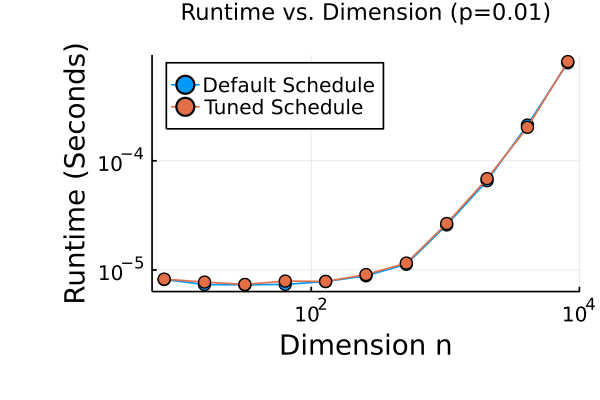
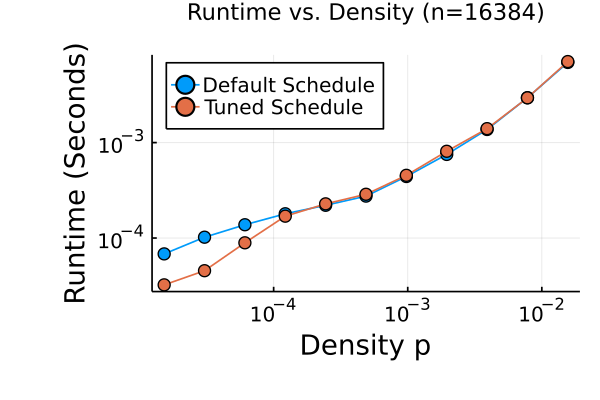
SpMV² $a_{i}=\sum B_{ij}\cdot C_{jk}\cdot d_{k}$

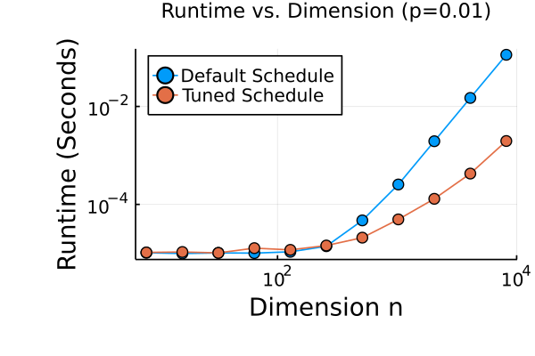
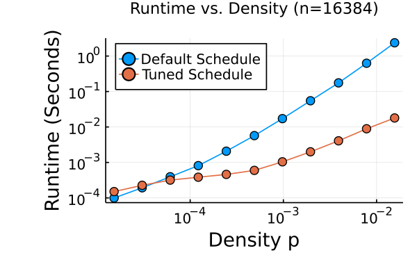
SpMTTKRP $A_{ij}=\sum B_{ikl}\cdot C_{kj}\cdot D_{lj}$

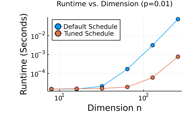
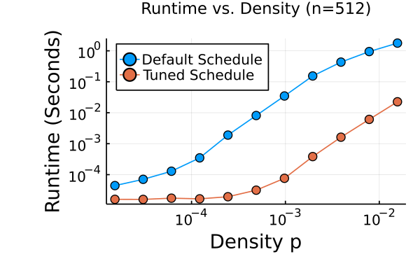
SpGEMM $A_{ij}=\sum B_{ik}\cdot C_{kj}$

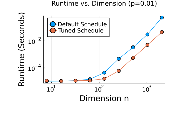
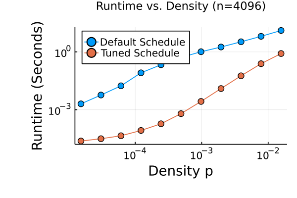
SpGEMM² $A_{ij}=\sum B_{ik}\cdot C_{kl}\cdot D_{lj}$

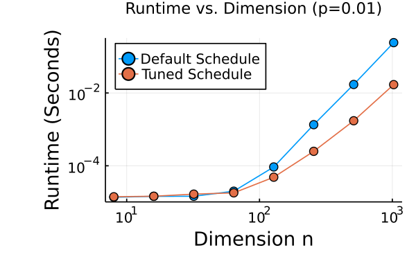
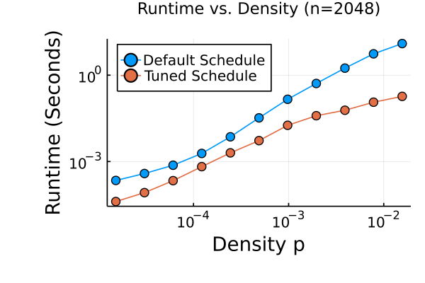
SpGEMMH $A_{ij}=\sum B_{ik}\cdot C_{kj}\cdot D_{kj}$

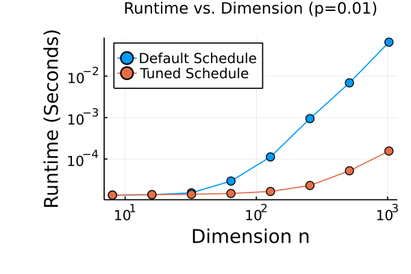
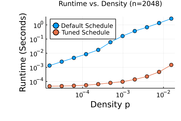
Figure 7. A comparison between the default schedule (nesting the loops in alphabetical order, without inserting any workspaces), and the schedule chosen by our autoscheduler on sparse inputs with uniformly random sparsity.

8. Related Work

Decades of research have been devoted to the online autoscheduling problem for sparse kernels, where optimizations are made to the kernel in response to the sparsity pattern of the inputs. Notable examples include the OSKI sparse kernel library (Vuduc, 2004) and similar efforts to use analytical cost models to choose between implementations, or more recent efforts to use machine learning to make these decisions (Dhandhania et al., 2021). A broad summary of similar efforts is given in (Strout et al., 2018a).

Our efforts differ from such approaches as our decisions are made offline, without examining matrix inputs. In the dense case, our problem looks quite similar to the tensor contraction ordering problem, where the most important cost function is simply the loop nesting depth and storage cost of dense temporaries (Gray and Kourtis, 2021; Schindler and Jermyn, 2020; Liang et al., 2021). However, since we consider the sparsity of our tensors and kernels, our algorithm is more similar to query optimizers for databases (Chandra and Merlin, 1977; Kolaitis and Vardi, 2000; Konstantinidis and Ambite, 2013), which use the theory of conjunctive query containment to reduce an input query to its smallest equivalent.

Other related work combines sparse tensor algebra and relational databases. Kotlyar et al. proposed implementing sparse tensor algebra using relational algebra and database techniques (Kotlyar, 1999; Kotlyar et al., 1997b, c, a), but did not give any techniques to optimize the generated code. It is unclear if these techniques would extend to the additional formats and operations proposed in (Chou et al., 2018; Henry et al., 2021). Yu et al. proposed integrating sparse matrix operations into relational queries, and proposed a few techniques to optimize the resulting join structures. However, this technique was not generalized beyond matrices, nor does it apply directly to tensor compilers and the kinds of programs they generate(Yu et al., 2021).

Set-like representations have been used before to describe implementations of tensor programs. The most popular example of this is the polyhedral framework, which represents the iterations of dense loops with affine loop bounds as abstract geometric polyhedra. We leave a summary of such prior work to (Baghdadi et al., 2019). The polyhedral model has been extended to the sparse case by Strout et al. (Strout et al., 2016; Strout et al., 2018b; Rift, 2021). However, the sparse polyhedral representations are used to describe the schedule itself, and not the complexity of the schedule. These sparse polyhedral representations have therefore not been used to automatically analyze or optimize the asymptotic complexity of program implementations.

9. Conclusions

Our cost model represents the first automatically derived expression of asymptotic complexity for sparse tensor programs. We describe algorithms to determine when one program asymptotically dominates another. Our enumerative autoscheduler can be used to produce a frontier of asymptotically sound skeleton programs as a starting point for further optimizations, such as parallelization or cache blocking.

Our cost model can be extended in several ways. By emitting set expressions for the tensor patterns, we can analyze the intermediate storage size of various tensor temporaries. By stratifying our tasks into multiple sets (e.g. a set for expensive tasks and a set for cheaper ones), we can begin to abstractly analyze some of the constant or logarithmic performance differences between, say, floating point operations and hash table operations. Our model can also be applied to programs with nonzero fill values or new semirings.

Our cost model also has applications beyond an enumerative autoscheduler. If better heuristics are to be developed for optimizing sparse tensor programs, our model can be used to evaluate them. Our model might also be used to guide a more sophisticated schedule search strategy, like greedy approaches, simulated annealing, or learning-based approaches. In the future, our offline techniques could be used to enhance online techniques, using runtime data to choose among the templates produced by the autoscheduler.

Sparse tensor compilers cannot expect end users to schedule their own programs. Automatic scheduling is necessary to fully abstract the details of sparse tensor compilation. The offline asymptotic decision making described in this paper is the last piece of infrastructure needed to make sparse tensor compilation accessible to the mainstream.

- (1)
- Abadi et al. (2016) Martin Abadi, Paul Barham, Jianmin Chen, Zhifeng Chen, Andy Davis, Jeffrey Dean, Matthieu Devin, Sanjay Ghemawat, Geoffrey Irving, Michael Isard, Manjunath Kudlur, Josh Levenberg, Rajat Monga, Sherry Moore, Derek G. Murray, Benoit Steiner, Paul Tucker, Vijay Vasudevan, Pete Warden, Martin Wicke, Yuan Yu, and Xiaoqiang Zheng. 2016. TensorFlow: A system for large-scale machine learning. In 12th USENIX Symposium on Operating Systems Design and Implementation (OSDI 16). 265–283. https://www.usenix.org/system/files/conference/osdi16/osdi16-abadi.pdf
- Adams et al. (2019) Andrew Adams, Karima Ma, Luke Anderson, Riyadh Baghdadi, Tzu-Mao Li, Michaël Gharbi, Benoit Steiner, Steven Johnson, Kayvon Fatahalian, Frédo Durand, and Jonathan Ragan-Kelley. 2019. Learning to optimize halide with tree search and random programs. ACM Transactions on Graphics 38, 4 (July 2019), 121:1–121:12. https://doi.org/10.1145/3306346.3322967
- Anderson et al. (2021) Luke Anderson, Andrew Adams, Karima Ma, Tzu-Mao Li, Tian Jin, and Jonathan Ragan-Kelley. 2021. Efficient automatic scheduling of imaging and vision pipelines for the GPU. Proceedings of the ACM on Programming Languages 5, OOPSLA (Oct. 2021), 109:1–109:28. https://doi.org/10.1145/3485486
- Arnold (2011) Gilad Arnold. 2011. Data-Parallel Language for Correct and Efficient Sparse Matrix Codes. PhD Thesis. University of California, Berkeley. 00000.
- Baghdadi et al. (2019) Riyadh Baghdadi, Jessica Ray, Malek Ben Romdhane, Emanuele Del Sozzo, Abdurrahman Akkas, Yunming Zhang, Patricia Suriana, Shoaib Kamil, and Saman Amarasinghe. 2019. Tiramisu: a polyhedral compiler for expressing fast and portable code. In Proceedings of the 2019 IEEE/ACM International Symposium on Code Generation and Optimization (CGO 2019). IEEE Press, Washington, DC, USA, 193–205.
- Bezanson et al. (2012) Jeff Bezanson, Stefan Karpinski, Viral B. Shah, and Alan Edelman. 2012. Julia: A Fast Dynamic Language for Technical Computing. arXiv:1209.5145 [cs] (Sept. 2012). http://arxiv.org/abs/1209.5145 arXiv: 1209.5145.
- Bik and Wijshoff (1993) Aart JC Bik and Harry AG Wijshoff. 1993. Compilation techniques for sparse matrix computations. In Proceedings of the 7th international conference on Supercomputing. ACM, 416–424. https://doi.org/10/dvjjwk 00000.
- Bik and Wijshoff (1994) Aart JC Bik and Harry AG Wijshoff. 1994. On automatic data structure selection and code generation for sparse computations. In Languages and Compilers for Parallel Computing. Springer, 57–75. 00000.
- Buluc and Gilbert (2008) Aydin Buluc and John R. Gilbert. 2008. On the representation and multiplication of hypersparse matrices. In 2008 IEEE International Symposium on Parallel and Distributed Processing. 1–11. https://doi.org/10.1109/IPDPS.2008.4536313 ISSN: 1530-2075.
- Chandra and Merlin (1977) Ashok K. Chandra and Philip M. Merlin. 1977. Optimal implementation of conjunctive queries in relational data bases. In Proceedings of the ninth annual ACM symposium on Theory of computing (STOC ’77). Association for Computing Machinery, New York, NY, USA, 77–90. https://doi.org/10.1145/800105.803397
- Chou et al. (2018) Stephen Chou, Fredrik Kjolstad, and Saman Amarasinghe. 2018. Format abstraction for sparse tensor algebra compilers. Proceedings of the ACM on Programming Languages 2, OOPSLA (Oct. 2018), 123:1–123:30. https://doi.org/10.1145/3276493
- Chou et al. (2020) Stephen Chou, Fredrik Kjolstad, and Saman Amarasinghe. 2020. Automatic generation of efficient sparse tensor format conversion routines. In Proceedings of the 41st ACM SIGPLAN Conference on Programming Language Design and Implementation (PLDI 2020). Association for Computing Machinery, New York, NY, USA, 823–838. https://doi.org/10.1145/3385412.3385963
- Dhandhania et al. (2021) Sunidhi Dhandhania, Akshay Deodhar, Konstantin Pogorelov, Swarnendu Biswas, and Johannes Langguth. 2021. Explaining the Performance of Supervised and Semi-Supervised Methods for Automated Sparse Matrix Format Selection. In 50th International Conference on Parallel Processing Workshop (ICPP Workshops ’21). Association for Computing Machinery, New York, NY, USA, 1–10. https://doi.org/10.1145/3458744.3474049
- Gray and Kourtis (2021) Johnnie Gray and Stefanos Kourtis. 2021. Hyper-optimized tensor network contraction. Quantum 5 (March 2021), 410. https://doi.org/10.22331/q-2021-03-15-410 Publisher: Verein zur Förderung des Open Access Publizierens in den Quantenwissenschaften.
- Gustavson (1978) Fred G. Gustavson. 1978. Two Fast Algorithms for Sparse Matrices: Multiplication and Permuted Transposition. ACM Trans. Math. Software 4, 3 (Sept. 1978), 250–269. https://doi.org/10.1145/355791.355796
- Henry et al. (2021) Rawn Henry, Olivia Hsu, Rohan Yadav, Stephen Chou, Kunle Olukotun, Saman Amarasinghe, and Fredrik Kjolstad. 2021. Compilation of sparse array programming models. Proceedings of the ACM on Programming Languages 5, OOPSLA (Oct. 2021), 128:1–128:29. https://doi.org/10.1145/3485505
- Kjolstad et al. (2019) Fredrik Kjolstad, Peter Ahrens, Shoaib Kamil, and Saman Amarasinghe. 2019. Tensor Algebra Compilation with Workspaces. In 2019 IEEE/ACM International Symposium on Code Generation and Optimization (CGO). 180–192. https://doi.org/10.1109/CGO.2019.8661185 ISSN: null.
- Kjolstad et al. (2017) Fredrik Kjolstad, Shoaib Kamil, Stephen Chou, David Lugato, and Saman Amarasinghe. 2017. The Tensor Algebra Compiler. Proc. ACM Program. Lang. 1, OOPSLA (Oct. 2017), 77:1–77:29. https://doi.org/10.1145/3133901
- Kolaitis and Vardi (2000) Phokion G. Kolaitis and Moshe Y. Vardi. 2000. Conjunctive-Query Containment and Constraint Satisfaction. J. Comput. System Sci. 61, 2 (Oct. 2000), 302–332. https://doi.org/10.1006/jcss.2000.1713
- Konstantinidis and Ambite (2013) George Konstantinidis and Jose Luis Ambite. 2013. Scalable containment for unions of conjunctive queries under constraints. In Proceedings of the Fifth Workshop on Semantic Web Information Management - SWIM ’13. ACM Press, New York, New York, 1–8. https://doi.org/10.1145/2484712.2484716
- Kotlyar (1999) Vladimir Kotlyar. 1999. Relational Algebraic Techniques for the Synthesis of Sparse Matrix Programs. PhD Thesis. Cornell. 00000.
- Kotlyar et al. (1997a) Vladimir Kotlyar, Keshav Pingali, and Paul Stodghill. 1997a. Compiling parallel sparse code for user-defined data structures. Technical Report. Cornell. 00000.
- Kotlyar et al. (1997b) Vladimir Kotlyar, Keshav Pingali, and Paul Stodghill. 1997b. A relational approach to the compilation of sparse matrix programs. In Euro-Par’97 Parallel Processing. Springer, 318–327. 00000.
- Kotlyar et al. (1997c) Vladimir Kotlyar, Keshav Pingali, and Paul Stodghill. 1997c. A relational approach to the compilation of sparse matrix programs. In Euro-Par’97 Parallel Processing (Lecture Notes in Computer Science), Christian Lengauer, Martin Griebl, and Sergei Gorlatch (Eds.). Springer, Berlin, Heidelberg, 318–327. https://doi.org/10.1007/BFb0002751
- Liang et al. (2021) Ling Liang, Jianyu Xu, Lei Deng, Mingyu Yan, Xing Hu, Zheng Zhang, Guoqi Li, and Yuan Xie. 2021. Fast Search of the Optimal Contraction Sequence in Tensor Networks. IEEE Journal of Selected Topics in Signal Processing 15, 3 (April 2021), 574–586. https://doi.org/10.1109/JSTSP.2021.3051231 Conference Name: IEEE Journal of Selected Topics in Signal Processing.
- McNamee (1971) John Michael McNamee. 1971. Algorithm 408: a sparse matrix package (part I) [F4]. Commun. ACM 14, 4 (April 1971), 265–273. https://doi.org/10.1145/362575.362584
- Mullapudi et al. (2016) Ravi Teja Mullapudi, Andrew Adams, Dillon Sharlet, Jonathan Ragan-Kelley, and Kayvon Fatahalian. 2016. Automatically scheduling halide image processing pipelines. ACM Transactions on Graphics 35, 4 (July 2016), 83:1–83:11. https://doi.org/10.1145/2897824.2925952
- Pugh and Shpeisman (1999) William Pugh and Tatiana Shpeisman. 1999. SIPR: A new framework for generating efficient code for sparse matrix computations. In Languages and Compilers for Parallel Computing. Springer, 213–229. 00000.
- Ragan-Kelley et al. (2013) Jonathan Ragan-Kelley, Connelly Barnes, Andrew Adams, Sylvain Paris, Frédo Durand, and Saman Amarasinghe. 2013. Halide: a language and compiler for optimizing parallelism, locality, and recomputation in image processing pipelines. In Proceedings of the 34th ACM SIGPLAN Conference on Programming Language Design and Implementation (PLDI ’13). Association for Computing Machinery, New York, NY, USA, 519–530. https://doi.org/10.1145/2491956.2462176
- Rift (2021) Anna Rift. 2021. Optimizing Scientific Computations with the Sparse Polyhedral Framework. 2021 Undergraduate Research Showcase (April 2021). https://scholarworks.boisestate.edu/under_showcase_2021/91
- Schindler and Jermyn (2020) Frank Schindler and Adam S. Jermyn. 2020. Algorithms for tensor network contraction ordering. Machine Learning: Science and Technology 1, 3 (July 2020), 035001. https://doi.org/10.1088/2632-2153/ab94c5 Publisher: IOP Publishing.
- Senanayake et al. (2020) Ryan Senanayake, Changwan Hong, Ziheng Wang, Amalee Wilson, Stephen Chou, Shoaib Kamil, Saman Amarasinghe, and Fredrik Kjolstad. 2020. A sparse iteration space transformation framework for sparse tensor algebra. Proceedings of the ACM on Programming Languages 4, OOPSLA (Nov. 2020), 158:1–158:30. https://doi.org/10.1145/3428226
- Strout et al. (2018a) Michelle Mills Strout, Mary Hall, and Catherine Olschanowsky. 2018a. The Sparse Polyhedral Framework: Composing Compiler-Generated Inspector-Executor Code. Proc. IEEE 106, 11 (Nov. 2018), 1921–1934. https://doi.org/10.1109/JPROC.2018.2857721 Conference Name: Proceedings of the IEEE.
- Strout et al. (2018b) Michelle Mills Strout, Mary Hall, and Catherine Olschanowsky. 2018b. The Sparse Polyhedral Framework: Composing Compiler-Generated Inspector-Executor Code. Proc. IEEE 106, 11 (Nov. 2018), 1921–1934. https://doi.org/10.1109/JPROC.2018.2857721 Conference Name: Proceedings of the IEEE.
- Strout et al. (2016) Michelle Mills Strout, Alan LaMielle, Larry Carter, Jeanne Ferrante, Barbara Kreaseck, and Catherine Olschanowsky. 2016. An approach for code generation in the Sparse Polyhedral Framework. Parallel Comput. 53 (April 2016), 32–57. https://doi.org/10.1016/j.parco.2016.02.004
- Tian et al. (2021) Ruiqin Tian, Luanzheng Guo, Jiajia Li, Bin Ren, and Gokcen Kestor. 2021. A High-Performance Sparse Tensor Algebra Compiler in Multi-Level IR. arXiv:2102.05187 [cs] (Feb. 2021). http://arxiv.org/abs/2102.05187 arXiv: 2102.05187.
- Venkat et al. (2015) Anand Venkat, Mary Hall, and Michelle Strout. 2015. Loop and Data Transformations for Sparse Matrix Code. In Proceedings of the 36th ACM SIGPLAN Conference on Programming Language Design and Implementation (PLDI 2015). 521–532. https://doi.org/10/ggwbwg 00000 event-place: Portland, OR, USA.
- Virtanen et al. (2020) Pauli Virtanen, Ralf Gommers, Travis E. Oliphant, Matt Haberland, Tyler Reddy, David Cournapeau, Evgeni Burovski, Pearu Peterson, Warren Weckesser, Jonathan Bright, Stéfan J. van der Walt, Matthew Brett, Joshua Wilson, K. Jarrod Millman, Nikolay Mayorov, Andrew R. J. Nelson, Eric Jones, Robert Kern, Eric Larson, C. J. Carey, İlhan Polat, Yu Feng, Eric W. Moore, Jake VanderPlas, Denis Laxalde, Josef Perktold, Robert Cimrman, Ian Henriksen, E. A. Quintero, Charles R. Harris, Anne M. Archibald, Antônio H. Ribeiro, Fabian Pedregosa, and Paul van Mulbregt. 2020. SciPy 1.0: fundamental algorithms for scientific computing in Python. Nature Methods 17, 3 (March 2020), 261–272. https://doi.org/10.1038/s41592-019-0686-2 Bandiera_abtest: a Cc_license_type: cc_by Cg_type: Nature Research Journals Number: 3 Primary_atype: Reviews Publisher: Nature Publishing Group Subject_term: Biophysical chemistry;Computational biology and bioinformatics;Technology Subject_term_id: biophysical-chemistry;computational-biology-and-bioinformatics;technology.
- Vuduc (2004) Richard W. Vuduc. 2004. Automatic performance tuning of sparse matrix kernels. Ph.D. Dissertation. University of California, Berkeley, CA, USA. http://bebop.cs.berkeley.edu/pubs/vuduc2003-dissertation.pdf
- Yu et al. (2021) Yongyang Yu, Mingjie Tang, and Walid G. Aref. 2021. Scalable Relational Query Processing on Big Matrix Data. arXiv:2110.01767 [cs] (Oct. 2021). http://arxiv.org/abs/2110.01767 arXiv: 2110.01767.