The GALAH Survey: Improving our understanding of confirmed and candidate planetary systems with large stellar surveys

Abstract

Pioneering photometric, astrometric, and spectroscopic surveys are helping exoplanetary scientists better constrain the fundamental properties of stars within our galaxy, and the planets these stars host. In this study, we use the third data release from the stellar spectroscopic GALAH Survey, coupled with astrometric data of eDR3 from the Gaia satellite, and other data from NASA’s Exoplanet Archive, to refine our understanding of 279 confirmed and candidate exoplanet host stars and their exoplanets. This homogenously analysed data set comprises 105 confirmed exoplanets, along with 146 K2 candidates, 95 TESS Objects of Interest (TOIs) and 52 Community TOIs (CTOIs). Our analysis significantly shifts several previously (unknown) planet parameters while decreasing the uncertainties for others; Our radius estimates suggest that 35 planet candidates are more likely brown dwarfs or stellar companions due to their new radius values. We are able to refine the radii and masses of WASP-47 e, K2-106 b, and CoRoT-7 b to their most precise values yet, to less than 2.3% and 8.5% respectively. We also use stellar rotational values from GALAH to show that most planet candidates will have mass measurements that will be tough to obtain with current ground-based spectrographs. With GALAH’s chemical abundances, we show through chemo-kinematics that there are five planet-hosts that are associated with the galaxy’s thick disc, including NGTS-4, K2-183 and K2-337. Finally, we show there is no statistical difference between the chemical properties of hot Neptune and hot rocky exoplanet hosts, with the possibility that short-period rocky worlds might be the remnant cores of hotter, gaseous worlds.

1 Introduction

Over the past three decades, new discoveries have moved the study of alien worlds from science fiction to science fact. We now know that planets are ubiquitous - that virtually every star in the sky is accompanied by a retinue of exoplanets (Batalha et al., 2013; Dressing & Charbonneau, 2013, 2015; Hsu et al., 2019; Kunimoto & Matthews, 2020; Yang et al., 2020). One of the great revelations of the first thirty years of the exoplanet era is the diversity exhibited by the physical properties of the planets we have discovered. We have found massive planets with extremely inflated, tenuous atmospheres, resulting in bulk densities lower than that of cotton candy (Rowe et al., 2014a; Dragomir et al., 2019; Deleuil et al., 2008; Siverd et al., 2012; Bailes et al., 2011), and others whose density far exceeds that of the planets in the Solar system (Steffen et al., 2013; Masuda, 2014; Zhou et al., 2017; Hartman et al., 2019; Rowe et al., 2014b; Lam et al., 2017; Hartman et al., 2016). Such studies have even revealed systems with similar-sized planets of very disparate mass – such as the Kepler-107 system; Kepler-107 b and c both have radii of $\sim$1.5R_⊕, but while b has an Earth-like density of 5.3 g cm^-3, c has a density at least twice as large, 12.6 g cm^-3; Bonomo et al. 2019).

In the coming years, our ability to determine the true mass and radius of newly discovered exoplanets will become even more important, as the search for exoplanets becomes a dedicated effort to find planets that could be considered truly ‘Earth-like’. Those planets will require significant effort to measure their atmospheres in an attempt to look for potential biomarkers. As a result, it will be vitally important to be able to work out which of those planets are most likely to be truly Earth-like (see e.g. Horner & Jones, 2010, , and references therein).

One of the key pieces of information for that selection process will be precise estimates of the mass and density of the planets in question – data that can be used to estimate the physical makeup and internal structure of those planets. However, the precision with which we can determine both the mass and the radius of a given planet is limited by the precision with which we can categorise that planet’s host star. The less precisely we know the mass or radius of that star, the less accurate will be the parameters we derive for the planets orbiting the star. Our knowledge of the worlds we discover is limited by our knowledge of their host stars.

The problem has become even more pronounced since the launch of TESS, which has already delivered a plethora of new discoveries (e.g. Huang et al., 2018; Nielsen et al., 2019; Vanderburg et al., 2019; Plavchan et al., 2020; Jordán et al., 2020; Addison et al., 2021; Rodriguez et al., 2021) along with candidate systems waiting for their planetary status to be confirmed, such as TESS Object of Interest (TOIs) and Community TOIs (CTOIs). Currently, the median error for TOI planetary radii is in excess of 10%. Fortunately, vast galactic archaeology surveys are now gathering high-quality spectroscopic data on hundreds of thousands of stars in the local solar neighbourhood, as well as stars within the galaxy’s thick and thin disks (Cui et al., 2012; Steinmetz et al., 2006; Majewski et al., 2017; Gilmore et al., 2012; De Silva et al., 2015). The GALAH (GALactic Archeology with HERMES) survey (De Silva et al., 2015; Martell et al., 2016; Buder et al., 2018, 2020) is one such program, with the aim of gathering high-quality spectra for up to one million nearby stars. In GALAH’s latest data release, GALAH DR3 (DR3; Buder et al., 2020), the GALAH team provide the results of their observations of 588,571 stars – including elemental abundances for up to 27 different elements. The resulting dataset is a treasure-trove of information that is of vital importance to the exoplanet community. In particular, the GALAH stellar abundances can assist in determining the compositions of the planets these stars might host (Bitsch & Battistini, 2020; Clark et al., 2020; Unterborn et al., 2018a; Dorn et al., 2017, 2015; Rogers & Seager, 2010), and even the types of planets the stars could potentially host (Hinkel et al., 2019). At the same time, the Gaia spacecraft is taking incredibly precise distance measurements of the stars being surveyed by GALAH (surveying up to $\sim$ 2% of all stars in the Galaxy).

In this work, we use data from the GALAH DR3 and Gaia EDR3 to refine the stellar parameters for a total of 273 stars in the TESS Input Catalog (TIC). We show how GALAH data can greatly improve the precision of our characterisation of potential planet hosting stars. Section 2 determines the stellar parameters for our sample and comparing them to our surveys. In section 3, we use these stellar parameters to then recharacterise confirmed and candidate planetary systems. We discuss our results in Section 4, identifying false positives, using our stellar $v\sin{i}$ values to determine how difficult it will be to determine mass measurements for our candidates, discuss the ultra-short period planets within our sample, confirm thick-disc host stars, compare the chemical abundances of hot Neptune and hot rocky worlds, and assess the radius valley and super-Earth desert of our sample. Finally we give our conclusions in Section 5.

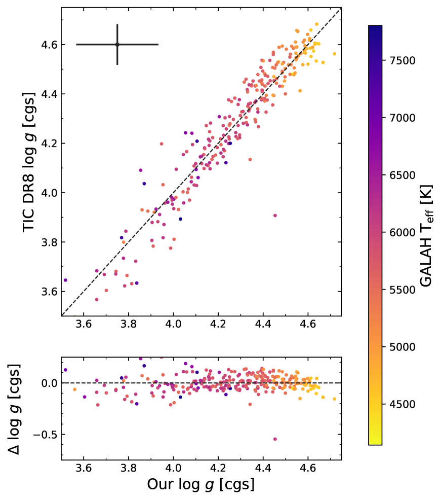
Figure 1: Left: GALAH DR3’s T${}_{\text{eff}}$ results are plotted against the T${}_{\text{eff}}$ measurements found within the Gaia DR2 (blue) and TIC (purple) catalogs respectively. An equality line (grey dashed) is plotted for comparison. Only stars within the TIC that were flagged as obtaining their effective temperature values from photometric surveys are plotted on this graph. A median GALAH-TIC and GALAH-Gaia T${}_{\text{eff}}$ error bars are found in the figure’s top left (purple and blue crosses respectively). Because the Gaia DR2 catalog currently does not produce errors for their T${}_{\text{eff}}$ values, there is no median y-error bar for Gaia in the plot. The differences in our results are plotted in the bottom plot with $\Delta$X = X_Other - X_GALAH. Right: GALAH’s log $g$ values compared to the TICs with each star colour-coded by their T${}_{\text{eff}}$ values. As with the T${}_{\text{eff}}$ figure to the left, an equality line (grey-dashed line) is shown along with the median TESS and GALAH log $g$ error bar shown in the top left (grey cross). log $g$ values for giant stars are not derived in the TIC and are thus not compared with GALAH’s values within this figure.

2 Determining Stellar Parameters

2.1 Combining Input Data

All three GALAH Data Releases (DR1; DR2; DR3; Martell et al., 2016; Buder et al., 2018, 2020, respectively) contain physical and chemical parameters for stars observed on the 3.9 m Anglo-Australian Telescope (AAT), situated on Gamilaraay land in New South Wales, Australia. There are 392 science fibres attached to the two degree-field prime focus top-end (2dF; Lewis et al., 2002) that feed into the High Efficiency and Resolution Multi Element Spectrograph (HERMES) (Sheinis et al., 2015), delivering high resolution (R $\approx$28,000) spectra in four distinct wavelength arms covering 471.3-490.3 nm, 564.8-587.3 nm, 647.8-673.7 nm and 758.5-788.7 nm respectively. Systematic and atmospheric effects are corrected for each spectrum and then continuum normalised with detailed physical parameters including T${}_{\text{eff}}$ , log $g$, [M/H] and individual abundances derived from each stellar spectrum using 1D stellar atmospheric models via the Spectroscopy Made Easy (or SME, Valenti & Piskunov, 1996) package.

2.1.1 GALAH DR3

GALAH DR3 is slightly different from its previous two counterparts (GALAH DR2; Buder et al. 2018, and DR1; Martell et al. 2016) in a few ways. Firstly, GALAH DR3 includes other stellar surveys, such as TESS-HERMES (Sharma et al., 2018) and K2-HERMES (Wittenmyer et al., 2018; Sharma et al., 2019), that have also used the AAT and HERMES instrument. This creates a catalog with more coverage across the ecliptic and southern ecliptic pole. It also creates a catalog that includes stars specifically observed for exoplanet detection and characterisation.

Secondly, GALAH DR3 solely uses SME to derive stellar parameters for all $\sim$600,000 stars, whereas SME was only used in a subset of stars within DR1 and DR2 with these results then propagated through the rest of the catalog thanks to The Cannon (Ness et al., 2015). Quality flags have been determined for each star, encoded as a bitmask with flags raised indicating various problems with the analysis. For our analysis, we only include stars within our analysis that had an SME flag flag_sp = 0, and also required the Fe abundance flag flag_X_fe = 0 in the GALAH DR3 release.

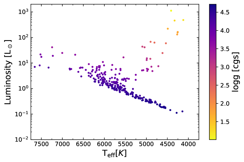
Figure 2: This Hertzsprung-Russell diagram of our GALAH DR3 T${}_{\text{eff}}$ and isochrones luminosity values colour-coded by GALAH DR3’s log $g$values, shows that the vast majority of planet-hosting or candidate-system stars lie on the main sequence. Of our 280 stars, only 21 are giants (T${}_{\text{eff}}$ $<$ 5500 and log $g$$<$ 3.5)

2.1.2 Cross-matching with other stellar and planetary catalogues

For our analysis, we firstly cross-matched GALAH DR3 with the TIC DR8 (Stassun et al., 2018), Gaia DR2 (Gaia Collaboration et al., 2018) and Gaia EDR3 (Gaia Collaboration et al., 2020) using the TOPCAT (Taylor, 2005) tool, cross-matching both catalogs with a position tolerance of $\pm$1″. Because we are interested in re-characterising confirmed or candidate exoplanetary systems, we then cross-matched GALAH DR3 with four different exoplanet and exoplanet candidate catalogs. These four catalogs include the NASA’s Exoplanet Archive (NEA), and exoplanetary candidates from the K2 and TESS missions. We cross-matched the NEA, and TESS TOI and CTOI catalogs by comparing their TIC identifiers with those found within our catalog, and cross-matched the K2 candidate list with our catalog by comparing 2MASS identifiers. We only accepted a K2 cross-match if the planet candidate was flagged as a “CANDIDATE" within the K2 Candidate Catalog, rejecting those which are already confirmed exoplanets, which would be picked up through the Exoplanet catalog cross-match, and already known false-positives. We have included all TOIs and CTOIs, regardless of their disposition currently described by the TESS Follow-up Observing Program Working Group (TFOPWG) within the TOI and CTOI catalogs. From this cross-matching, we have identified 280 stars within GALAH DR3 that either host confirmed or candidate exoplanets.

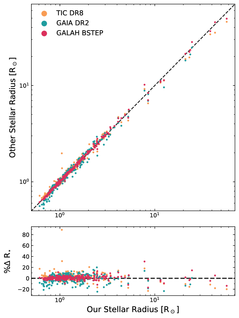
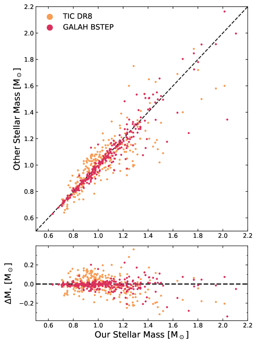
Figure 3: Left: Our stellar radius values are compared to other surveys and methodologies to confirm the validity of our values. Radius values derived from isochrones are compared with values found within the TIC (yellow), Gaia DR2 (blue) and GALAH’s BSTEP VAC (red). Error bars are suppressed for clarity. An equality line in both plots is depicted in a grey dashed line. Right: Our stellar mass values are compared against those that are found within the TIC (yellow) and GALAH’s BSTEP VAC (red). 1-$\sigma$ median error bars for each comparison can be found in the top-right corner of the figure.

2.2 Stellar Masses, Radii, Luminosities, Ages via Isochrones

To derive the physical parameters of these host stars from the GALAH catalog, we use a similar approach to Clark et al. (2020), implementing the Python package isochrones (Morton, 2015). isochrones derives physical parameters from observed stellar parameters using the stellar evolution grid, MESA Isochrones & Stellar Tracks (MIST; Choi et al., 2016). For our analysis, we used the star’s effective temperature (T${}_{\text{eff}}$ ), surface gravity (log $g$) and colour excess (E(B-V)) from GALAH, Johnson-Morgan ($V$; taken from the TIC), 2MASS ($J$, $H$, $K_{s}$) and Gaia EDR3 ($G$, $G_{RP}$, $G_{BP}$) photometric magnitudes, along with parallax values obtained by Gaia EDR3 (Gaia Collaboration et al., 2020) where available as input observables for isochrones. We incorporated the associated errors for each measurement from their respective catalogs but inflated the associated errors in the photometric bands to 0.05 mag. By inflating the magnitude errors rather than including their associated errors, we found the stars to better converge on more realistic results, with isochrones producing better estimates on the error of the derived parameters. We also include the star’s global metallicity, [M/H], derived by GALAH’s [Fe/H] and [$\alpha$/Fe] abundances formulated by Salaris & Cassisi (2006) as:

$$\mathrm{[M/H]=[Fe/H]}+\log_{10}{\big{(}0.694f_{\alpha}+0.306\big{)}}\,\,,$$ (1)

where $f_{\alpha}$ is the $\alpha$-element enhancement factor given by $f_{\alpha}=10^{\left[\frac{\alpha}{Fe}\right]}$. When the model reaches convergence, the median and corresponding 1-$\sigma$ uncertainties for stellar mass, radius, density, age, and equivalent evolution phase values are calculated from their respective posterior distributions. A star’s stellar luminosity is then calculated through the Stefan-Boltzmann relationship, with these resulting luminosities used to derive the habitable zone boundaries for each star, as formulated by Kopparapu et al. (2013). We include all five HZ boundaries within Kopparapu et al. (2013) including Recent Venus, Runaway Greenhouse, Moist Greenhouse, Maximum Greenhouse and Early Mars. Rotational, radial and microturbulence velocities from GALAH DR3 have also been included in our stellar parameter table (Table 4), to assist ground-based radial velocity teams to better prioritise follow-up targets, including K2, TOI and CTOI candidates.

Table 1: Median and 1$\sigma$ values of our exoplanet/candidate-hosting population

Quantity	$\mu\pm\sigma$
T${}_{\text{eff}}$  [K]	5633 $\pm$ 88
log $g$ [cgs]	4.28 $\pm$ 0.19
[Fe/H] [dex]	-0.01 $\pm$ 0.08
[$\alpha$/Fe] [dex]	0.02 $\pm$ 0.04
[M/H] [dex]	0.03 $\pm$ 0.10
R⋆ [R⊙]	1.18 $\pm$ 0.03
M⋆ [M⊙]	1.02 $\pm$ 0.04
L⋆ [L⊙]	1.49 $\pm$ 0.11
Age [Gyr]	4.98 $\pm$ 2.90

2.3 Comparison of Stellar Parameter estimates

Because our methodology uses cross-matched data with Gaia DR2 and TIC DR8, we can use stellar parameter values from these catalogs to determine any biases from our own data. The median value and median 1-$\sigma$ errors for our stellar parameters can be found in Table1 with the full stellar parameter catalog being found in Table 4. Figure 1 shows the comparison of GALAH DR3 log $g$ and T${}_{\text{eff}}$  values with those determined by Gaia and the TIC.

2.3.1 Stellar T${}_{\text{eff}}$ 

There is an overall good agreement between the catalogs, with a mean difference between Teff values from GALAH and TIC of $-11^{+121}_{-127}$ K, and Gaia of $32^{+281}_{-163}$ K, with an RMS difference of 10 and 21 K, respectively. Just as Hardegree-Ullman et al. (2020) and Clark et al. (2020) showed in their work, we also find a horizontal structure within our Gaia T${}_{\text{eff}}$  comparison near 5000 K. This further suggests that Gaia T${}_{\text{eff}}$  values preferentially converge onto some T${}_{\text{eff}}$ values over others. For our comparison of TIC T${}_{\text{eff}}$  values, we only compare GALAH’s values to those found with the TIC that have been derived photometrically and not spectroscopically. This is to avoid the potential comparison of GALAH DR2 values, as the TIC incorporated GALAH DR2’s T${}_{\text{eff}}$  measurements into their catalog. Our median planet-hosting temperature of 5514 K is slightly cooler than candidate-hosts with a median temperature of 5698 K.

2.3.2 Stellar log $g$

Because the Gaia catalog contains no log $g$ values for their stellar catalog, we only compare our log $g$ results to those found within the TIC. In its current iteration, the TIC has log $g$ values for only dwarf stars and not giants, to fit within the science requirements of the TESS mission. Figure 1 also shows the comparison with our dwarf log $g$ values to those found in the TIC. There is a strong overall agreement with our log $g$ values and those found within the TIC with a bias and RMS of ${0.00}^{+0.06}_{-0.08}$ and 0.01 dex respectively. Only one star seemed to be a significant outlier with the CTOI-host star TIC 179582003 having a log $g$ of 4.45$\pm$0.19 dex compared to a slightly lower surface gravity found within the TIC of 3.91$\pm$0.08 dex.

2.3.3 Stellar [M/H]

Overall metallicity values, [M/H], are found within Table 4 and were calculated from GALAH DR3’s [Fe/H] and [$\alpha$/Fe] abundances. We should note that the current TIC catalog directly incorporates GALAH DR2’s iron abundances, [Fe/H], as a star’s overall metallicity, [M/H]. As such, a direct comparison between such values is left to a more thorough analysis of iron abundance improvements from DR2 and DR3 in (Buder et al., 2020).

2.3.4 Stellar Radius and Mass

From GALAH’s DR3 T${}_{\text{eff}}$ , log $g$ and [M/H] measurements, alongside photometric and astrometric parameters, we have been able to constrain stellar mass, radius, age and thus luminosity values from isochrones. For a sanity check, we created a Hertzsprung-Russell diagram found in Figure 2 to check if our stars fell into any nonphysical areas of the diagram. A vast majority of our planet-hosting or candidate hosting stars lie on the main sequence with only 21 giant stars within our sample (Note, we classify a star as a giant, by it being cooler than 5500 K and having a surface gravity of less than 3.5; Sharma et al. 2019).

Figure 3 compares our stellar radius and mass values against other internal and external catalogs. Our stellar radius values are compared against those found within the TIC, Gaia DR2 and the GALAH DR3 BSTEP Value Added Catalog (VAC). The BSTEP VAC results for K2-HERMES and TESS-HERMES stars are being released in a future paper. Briefly, stellar parameters such as age, mass and radius were computed with the BSTEP code (Sharma et al., 2018) making use of PARSEC-COLIBRI stellar isochrones (Marigo et al., 2017). BSTEP provides a Bayesian estimate of intrinsic stellar parameters from observed stellar parameters by making use of stellar isochrones. It is unsurprising, given the same data and similar methodology, that our stellar radius values agree well against those found in BSTEP, with a stellar radius bias and RMS of $-0.01^{+0.03}_{-0.04}$R_⊙ and 0.04R_⊙ respectively. These values are comparable to comparisons we make to the TIC and Gaia DR2, with median biases of $-0.02^{+0.05}_{-0.08}$ R_⊙  and $-0.01^{+0.09}_{-0.07}$ R_⊙ , and RMS values of 0.06 R_⊙  and 0.02 R_⊙ respectively.

While GALAH DR3 does not come with stellar masses, the BSTEP VAC catalog does, such that our isochrone derived results are compared with BSTEP and the TIC values found in Figure 3. There are 25 stars within our sample that have no mass measurements found within the TIC (including confirmed planet hosts K2-97 b (Livingston et al., 2018b), NGC 2682 Sand 364 b (Stassun et al., 2017) and NGC 2682 Sand 978 b (Brucalassi et al., 2017)), due to the TIC only deriving masses for dwarf stars and hence no comparison between their masses are shown in Figure 3.

As with the stellar radii, there seems to be an overall good agreement with our derived mass values and those found within the TIC, with a bias and RMS of $0.01^{+0.11}_{-0.09}$M_⊙ and 0.01M_⊙ respectively. Our stellar mass results are comparable with stellar mass values found in GALAH’s BSTEP VAC, with bias of $0.01^{+0.04}_{-0.03}$M_⊙  and RMS of 0.01M_⊙ respectively. However, there seems to be a larger scatter for stars more massive than 1.4M_⊙, with our results preferentially favouring larger mass values compared to the other catalogs. These mass and radius measurements become fundamental parameters for constraining the mass and size of the planets they host, which will be discussed in the next section.

3 Refining Planetary Systems

With our new stellar parameters, we can now refine and redetermine the planetary or potential planetary systems that these stars host. We previously cross-matched GALAH DR3 with the NEA for known planet-hosts and K2-candidates. We also cross-matched GALAH DR3 with stars known to host TOI and CTOIs. From these cross-matches, we have 105 confirmed exoplanets, and 293 exoplanet candidates with 146 K2 candidates, 95 TOIs and 52 CTOIs. The refined planetary parameters can be found in Table 5.

As there are multiple catalogs with differing definitions of transit depth (i.e some report it in mmag, others as a percentage or as $(R_{s}/R_{p})^{2}$), we convert all transit depths to percentages. Thus the exoplanet’s radius is defined by:

$$\frac{R_{p}}{R_{\oplus}}=\sqrt{0.01\Delta F}\frac{R_{s}}{R_{\odot}}\,\,,$$ (2)

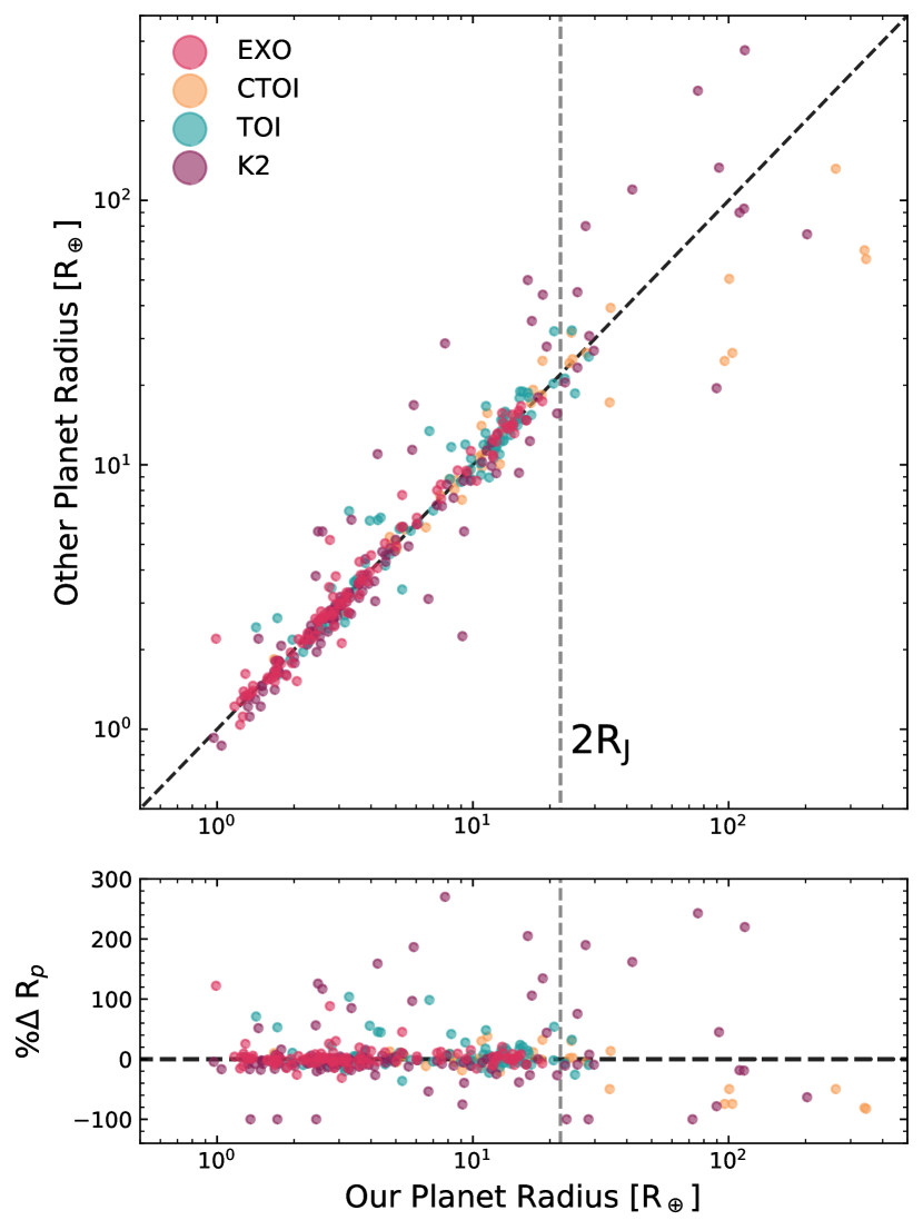
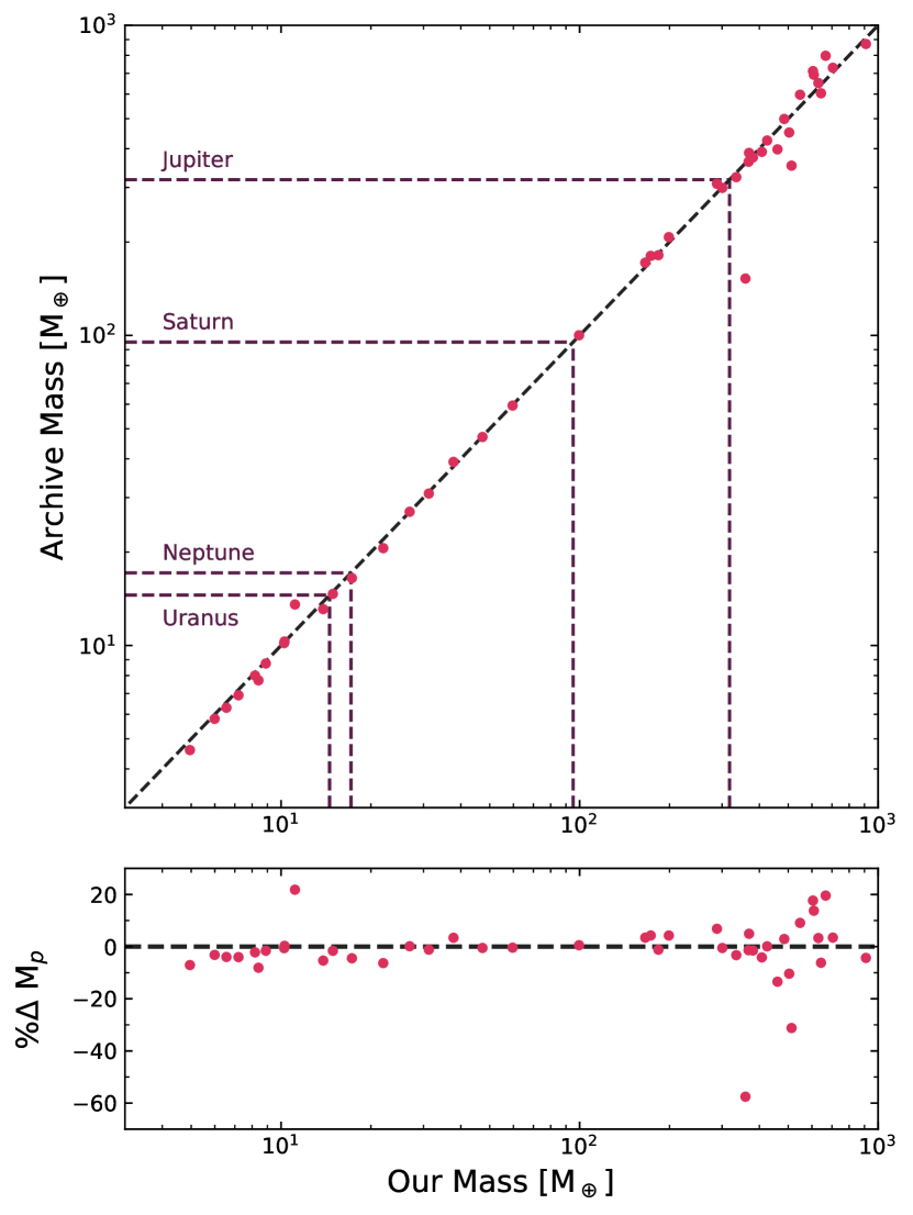
Figure 4: Left: Our planetary radii values are compared with literature values found within the NEA (red) K2 candidate catalog (purple) and TOI (blue) and CTOI (yellow) catalogs found on ExoFOP. No confirmed exoplanet thus far has a radius larger than twice that of Jupiter’s (vertical grey-dashed line). As such, any candidate beyond the right of this line is most likely non-planetary in nature and more likely a sub-stellar or stellar companion to its host star. Right: We compare our planetary mass values to those found within the NEA. Lines representing the masses of Uranus, Neptune, Saturn and Jupiter are depicted as purple dashed lines across the plot.

where $R_{p}$ is the planet’s radius, $\Delta F$ is the percentage transit depth and $R_{s}$ is the host star’s radius. The planet’s semi-major axis is calculated by Kepler’s third law, incorporating our revised stellar mass values. These semi-major axis values were then used alongside stellar luminosities ($L_{\star}$) to derive insolation flux values, S_eff, for each confirmed and candidate exoplanet. These stellar luminosities and the newly derived temperatures can then be used to determine a planet’s effective temperature. If an exoplanet’s atmosphere is “well-mixed", that being there is no obvious phase function at IR wavelengths, its effective temperature will be:

$$T_{p}=\bigg{(}\frac{L_{\star}(1-A)}{\alpha\pi\sigma r^{2}}\bigg{)}^{\frac{1}{4}}$$ (3)

where, $\alpha$ = 16, the spherical (Bond) albedo is given by A, $\sigma$ is the Stefan-Boltzmann constant and r is the star-planet separation which we’ve defaulted to be the semi-major axis (Kane & Gelino, 2011) of the star-planet system. For a hot-dayside exoplanet, whereby its atmosphere is inefficient with respect to heat distribution, its effective temperature is calculated also using Equation 3, but in this instance $\alpha$ = 8 instead (Kane & Gelino, 2011). Because an exoplanet’s rotational period (exo-day) is currently difficult to determine, we have included both values within Table 5.

We have used the geometric albedos from Sheets & Deming (2017) with geometric albedos assumed to be 0.11$\pm$0.06, 0.05$\pm$0.04, and 0.11$\pm$0.08 for planets 1–2 R_⊕, 2–4 R_⊕and 4–6 R_⊕, respectively. Bond albedos are then calculated from these geometric albedos using the relationship $A_{B}=3A_{g}/2$ (Seager, 2010). We also used the 1–2 R_⊕ albedo value for planets $R_{p}<1R_{\oplus}$ and used the Bond albedo value of 0.35$\pm$0.05 (Mallonn et al., 2019) for planets $>$6 R_⊕.

For known exoplanets that have measured line-of-sight, $M_{P}\sin i$, or true mass measurements, we refine their masses given our stellar mass values given by the formula:

$$\frac{M_{P}\sin i}{M_{\oplus}}=\frac{K_{RV}\sqrt{1-e^{2}}}{0.0895\mathrm{ms}^{-1}}\left(\frac{M_{*}}{M_{\odot}}\right)^{2/3}\left(\frac{P}{\mathrm{yr}}\right)^{1/3}$$ (4)

where $K_{RV}$ is the radial velocity’s semi-amplitude in ms^-1, $e$ is the orbital eccentricity and $P$ is the orbital period. This equation also assumes that M_p $\ll$ M_⋆ (Lovis & Fischer, 2010). If the orbital inclination of the system is known, we then refine the planet’s true mass, $M_{p}$.

Because the NEA is designed now to have multiple entries for a single exoplanet or planetary system, the challenge then becomes what observables we use to refine and re-characterise these exoplanets and planetary systems. We have used a weighted mean approach to determine a single value for our K2 candidate transit depths and orbital inclinations. We have also used a weighted mean approach to derive exoplanet transit depths, radial velocity semi-amplitudes, and orbital eccentricities, inclinations and periods where available. The weighted mean of observable $X$ is calculated by:

$$\bar{X}=\frac{\sum_{i=1}^{n}{w_{i}X_{i}}}{\sum_{i=1}^{n}{w_{i}}}$$ (5)

where the weight of the ith data point $w_{i}$ is related by its error, $\sigma_{i}$ as $w_{i}=\sigma_{i}^{-2}$. The error in the standard mean is then calculated to be:

$$\sigma_{\bar{X}}=\left(\sqrt{\sum_{i=1}^{n}{w_{i}}}\right)^{-1}$$ (6)

These weighted mean values are then used to refine the planetary mass and radii values found in Figure 4 with our new planetary properties found in Table 5.

4 Discussion

4.1 Identifying False Positives

Figure 4 shows the comparison of our planetary radii and mass values compared to catalog values found either on the NEA or NASA’s ExoFOP databases. If there were multiple planetary mass or radius values, we have compared our results to the latest values within their respective databases. Using the same definition found in Wittenmyer et al. (2018), we use an upper limit of R_P < 2 R_J $\approx$ 22R_⊕ for a planetary object. We have used this cut off as there is currently no confirmed exoplanet on the archive with a planetary radius larger than this value.

There are twelve CTOIs that have radii comparable to sub-stellar and stellar objects, being larger than our 2R_P limit. Of these Clark et al. (2020) also found the planetary radii values for CTOI 201256771.01, CTOI 201256771.02 and CTOI 300903537.01 to be too large for a planetary object. The two candidates orbiting TIC 141622065 both have radii of 344.62$\pm$6.50R_⊕ and 339.57$\pm$6.40R_⊕, with an orbital period separation of 0.05 days. These two candidate events are more akin to a single 3R_⊙ binary star companion. Similarly, the radii for all candidates in the CTOI 91369561 system including TIC 91369561.02 and TIC 91369561.03 have radii comparable to FGK type stars. CTOI 140830390.01 and CTOI 220402290.02 have planetary radii on the cusp of the “planetary-limit" of $\sim$22R_⊕ , but was further suggested in Clark et al. (2020) that the candidate events within the CTOI 220402290 system are also from a single object, which is likely caused by a sub-stellar or stellar companion. CTOIs 31869740.01 and 219322317.01 are both recorded as having sub-stellar radius values of 31.61R_⊕  and 39.24$\pm$2.64R_⊕  respectively on TFOP. With our revised radius values, these two candidates also have nonphysical planetary radii, with their radii now being 24.27$\pm$2.13R_⊕  and 34.59$\pm$0.71R_⊕  for CTOI events 31869740.01 and 219322317.01 respectively. Planetary candidate CTOI 140830390.01, also known as TOI 1072.01, is more likely a brown-dwarf with a planetary radius of 27.91 $\pm$ 0.68R_⊕. These results highlight the need for vetting of CTOI systems before they are made publicly available.

With our refined radii, there are five exoplanetary TOI candidates that have radii $R_{p}>2R_{J}$. These being TOI 147.01, 565.01, 959.01, 1072.01 and 2391.01. The TESS Follow-up team contains five specialist sub-groups, with TFOP Science Group 1 (SG1) specialising in seeing limited photometry. Members attempt to confirm and refine orbital parameters from TOIs, with the project lead then up- or down-ranking the candidates’ disposition depending upon their follow-up observations. Currently, TOI 147.01 and TOI 959.01 have their dispositions labelled as ‘False Positives’, with our work also confirming that their radii alone are too big to be considered planetary in nature. TOI 565.01 was originally labelled as a ‘False Positive’ under the TFOPWG Disposition in April 2019 but is now an ‘Ambiguous Planetary Candidate’ as of November 2020. With an archive planetary radius of 18.62R_⊕  and now an updated radius of 25.07$\pm$0.65R_⊕, this candidate is also now too large to be exoplanetary in nature and is likely an eclipsing binary event.

There are only two TOIs above our planetary radius limit, TOI 1072.01 and TOI 2391.01, which are currently labelled as Potential Candidates on TFOP, with TOI 1072.01’s planetary nature already being discussed. TOI 2379.01 is on the border-line of our defined planetary radii boundary, having a radius of 21.21$\pm$1.34R_⊕  on TFOP with our radius only being slightly higher of 22.89$\pm$0.58R_⊕. Notes on TFOP suggest that this event is likely an eclipsing binary, with our revised radii also being too large for a planet-like event. If confirmed to be an exoplanet, however, it would be one of the largest ever to be discovered.

There are 18 K2 candidates that have problematic radii with 13 having been found to be false positives in previous work (Wittenmyer et al., 2018, 2020). Of the five K2 candidates remaining, three candidates EPIC 210769880.01, EPIC 205050711.01 and EPIC 204546592.01 all have candidate radii $>$0.35R_⊙ , which far exceeds the physical radius needed to be a planetary event. There are two candidate events observed by K2 that are much closer to having radii nearer to the 2$R_{J}$ radius limit, these being EPIC 214611894.01 and EPIC 210598340.01.

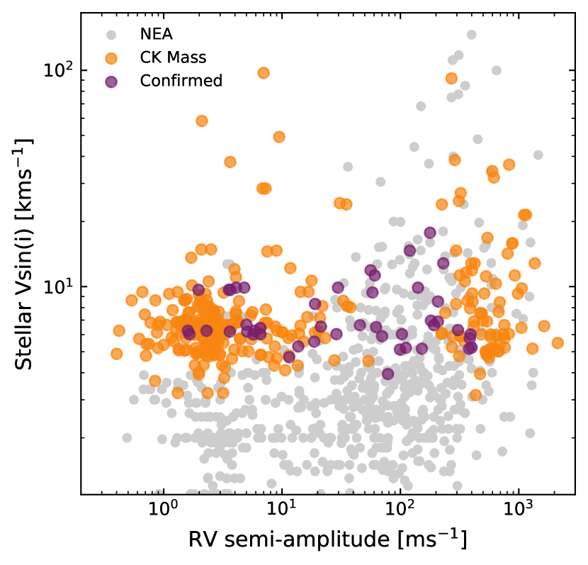
Figure 5: Expected radial velocity amplitudes for candidate and known exoplanets have been derived from expected mass values from Chen & Kipping (2017) (in yellow) and compared to exoplanets with known mass values in our sample (purple) and those within NASA’s Exoplanet Archive (grey)

EPIC 214611894.01 is a candidate event discovered through K2’s seventh campaign by Petigura et al. (2018) with a candidate radius of 20.5${}^{+2.8}_{-2.1}$R_⊕. Its refined stellar host radius of 1.35$\pm$0.02R_⊙  is larger compared to Petigura et al. (2018)’s value of 1.21R_⊙. This increase has meant the candidate’s radius is now 28.50$\pm$0.63R_⊕ , which is too large to be planetary in nature. A candidate first announced by Barros et al. (2016), EPIC 210598340.01’s radius was first determined by Kruse et al. (2019) as being 30.71${}^{+0.54}_{-6.89}$R_⊕. Our newly revised candidate radius for EPIC 210598340.01 sits right on our defined radius limit, being 22.92$\pm$0.45R_⊕ . This candidate radius is also smaller than the one derived by Hardegree-Ullman et al. (2020), with their derived planetary radius for EPIC 210598340.01 of 26.764${}^{1.724}_{-1.633}$R_⊕. With our revised radii, it is possible that this candidate is planetary in nature, but more follow-up is needed.

4.2 Follow up and mass confirmation from ground-based surveys

TESS is delivering thousands of candidate exoplanets in which the community will have to confirm and characterise by both space and ground based observations. The radius measurements of these candidates will be derived mostly from TESS photometry, with confirmation mass measurements being derived from ground-based radial velocity followup. On the the biggest considerations for radial velocity followup is considering a star’s rotational velocity - or in most cases, its projected rotational velocity ($v\sin{i}$). Slow rotating stars are the most preferred stellar companions, as they generally have well-defined absorption lines. As $v\sin{i}$ increases, the absorption lines needed for high-precision radial velocity measurements will broaden out, with some lines blending completely. This broadening decreases the number of well defined lines needed to obtain better radial velocity measurements, thus deteriorating the radial velocity precision. We have thus included $v\sin{i}$ values in Table 4 to assist followup teams in better allocating telescope time to feasible RV targets.

We have decided to forward model the likely mass and thus predicted radial velocity semi-amplitudes for confirmed and candidate exoplanets within our sample, to check which are the most viable targets for mass confirmation. To model the predicted radial velocity semi-amplitudes, we have used the Chen & Kipping (2017) mass-radius relationship to derive predicted mass values for exoplanets for which there exists no current mass measurements. From this, we have used Equation 4, along with the host’s stellar mass, the predicted planetary mass, observed orbital period and assuming circular orbits for these planets, to then obtain the predicted semi-amplitudes. These predicted semi-amplitude values are plotted against the host star’s $v\sin{i}$ in Figure 5. In Figure 5, we have also included confirmed exoplanets with known mass measurements from NEA for comparison to our predicted RV values.

For the majority of our candidates, their host star’s $v\sin{i}$values are above 5$kms^{-1}$, however the planet’s predicted RV signal is less than 5$ms^{-1}$. For context, only 19 confirmed exoplanets have RV signals less than 5$ms^{-1}$ orbiting stars with $v\sin{i}$ values greater than 5$kms^{-1}$. We then predict that it will be difficult, with current methodology, to obtain mass confirmations for most of the smaller planet candidates orbiting stars found within our sample. In the extreme cases for smaller planets orbiting rapid-rotating stars, it will be highly improbable to derive their mass measurements.

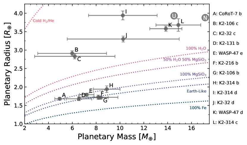
Figure 6: Revised planetary mass and radius values for confirmed super-Earth and mini-Neptune exoplanets within our sample. Each planet is labelled alphabetically, with its corresponding name to the right of the plot. 1-$\sigma$ error bars are given for each exoplanet, with Uranus and Neptune depicted on the plot as ’U’ and ’N’ in the plot’s right-hand corner. The mass-radius relationships used for the dashed lines to show density curves for cold H₂/He, 100% water, 50% water-50%rocky, pure rocky (containing pure post-perovskite MgSiO₃), "Earth-like" (33%Fe and 67%rock) and pure iron worlds are from (Zeng et al., 2016).

For example, the star TOI-1219 (TIC 294981566,) is a rapidly rotator ($v\sin{i}$ = 58.3 $\pm$ 2.5$kms^{-1}$) with a 1.97 $\pm$ 0.13R_⊕ planet candidate orbiting around it every 1.91 days. We wanted to see what the expected radial velocity precision would be for such candidate orbiting around such a rapid rotator, and compare that to the expected RV signal of the exoplanet. To do this, we created a template spectrum that roughly matched the stellar properties of the host star, resampling the spectrum to match modern extreme precision radial velocity (EPRV) spectrographs (Spectral range = 400–650 nm, R $\sim$ 100,000 and 3.5 pixels per FWHM). We then recreated this stellar template for its observed $v\sin{i}$ value, calculating the intrinsic error in radial velocities using (Butler et al., 1996). With its current rotational velocity, the expected RV precision for TOI-1219 is 20.5 $ms^{-1}$, nearly an order of magnitude difference compared to the predicted RV signal of TOI-1219.01 being an estimated 2.1 $ms^{-1}$. Since we know what the expected RV signal of the planet candidate is predicted to be (K = 2.1 $ms^{-1}$) and have an intrinsic RV precision ($\sigma_{\bar{V}}$ = 20.5 $ms^{-1}$) we can use the formula found in Wittenmyer et al. (2011):

$$N=\bigg{(}\frac{12.3\times\sigma_{\bar{V}}}{K+0.02}\bigg{)}^{2}\,\,,$$ (7)

to then determine the number of observations (N) needed to detect the radial velocity signal of TOI-1219.01. In this case, the number of observations needed to confirm the mass measurement of TOI-1219.01 would be over 14,000. For context, the number of radial velocity observation we currently use for RV detection is in the order of tens or in some case nearing to hundred or two hundred observations. Thus, for a relatively hot (T${}_{\text{eff}}$ = 6600 K) and rapidly rotating star, the precision needed to obtain a 3-sigma RV signal for TOI-1219.01 is unobtainable with current technology and methodology. Higher resolution spectrographs will be needed to determine the mass measurements of small planets orbiting rapid rotating stars. For reference, there is only one exoplanet that has a confirmed mass-measurement smaller than 4R_⊕  orbiting a star with a $v\sin{i}$ greater than 20$kms^{-1}$, with Kepler-462 b’s mass being determined through transit timing variations orbiting the rapid rotating star ($v\sin{i}$= 80 $\pm$ 3 $kms^{-1}$) Kepler-462 (Masuda & Tamayo, 2020). Transit timing variations can therefore be another great avenue to determine the mass measurements of these candidates, rather than utilising RV measurements. Our data, along with other large stellar surveys, then provides a useful database for ground-based followup teams to determine what are the most suitable targets to follow up for mass confirmation, to maximise their resource efficiency.

4.3 Planetary compositions from Mass-Radius Relations

4.3.1 Our results

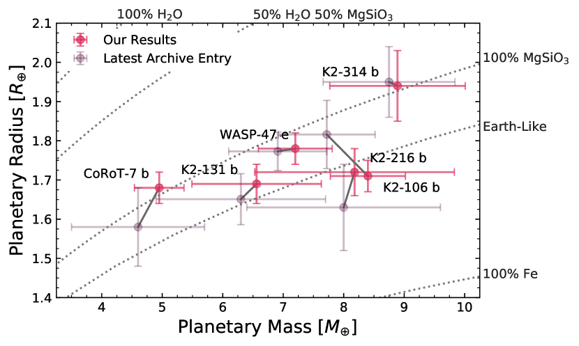
Figure 7: Combining the weighted mean and updated stellar parameters approach of our work (labelled as red crosses) has improved the mass and radius errors on several exoplanets that are thought to be rocky in nature within our work. The latest entry within the NEA is shown for reference as grey crosses.

Within GALAH’s latest data release, there are 105 confirmed planet-hosting stars. There was only one planet that was omitted in our analysis, this being the exoplanet Pr0211 c, as its orbital period error was too large to facilitate in the MCMC analysis of our work. With our previous line of thought, there are no planets with revised radii measurements that exceed the 2$R_{J}$ limit. Nor do any revised mass measurements, where available, exceed the theoretical exoplanet mass limit of $\sim$13$M_{J}$ (Boss, 2001). Figure 4 shows our newly derived mass values compared to those found in the literature. We should note that in Figure 4, the comparison of literature values are median mass and radius values taken from the NEA. There are three visible outliers within the comparison mass plot, CoRoT-7 c (11.12$\pm$0.79M_⊕), K2-97 b (359.26$\pm$38.56M_⊕) and K2-34 b (512.48$\pm$17.39M_⊕). With further inspection, these three outliers are mainly caused by various anomalies within the NEA, rather than drastic changes with the refined stellar parameters, for example, K2-97 b.

An example of the caveats of both our methodology and utilising any form of heterogeneous archival data comes from the revision of planetary system K2-97. First discovered by Grunblatt et al. (2016), K2-97 b is a Jupiter-sized exoplanet that had an initial radial velocity semi-amplitude of 103$\pm$8 ms^-1, inferring a planetary mass of 350$\pm$35M_⊕, where our refined value is 359.26$\pm$38.56M_⊕.

However, its radial velocity semi-amplitude was later revised by Grunblatt et al. (2017) through additional radial velocity measurements to be 42.1${}^{+4.3}_{-4.2}$ ms^-1, a decrease of over 56%. These new measurements imply a revised mass of 153$\pm$22M_⊕. But this RV value is not included within the NEA, and hence wasn’t used within our methodology until now.

If these literature values were treated as independent measurements, our weighted mean approach would yield an estimated mass for K2-97 b of 146.7$\pm$18.4M_⊕. But, if you then incorporate both of these values in our weighted mean approach, the mass of K2-97 b then becomes 194.54$\pm$19.54M_⊕. Additionally, if we were only to use the default parameters (default_flag) used by the NEA, K2-97 b’s parameters would include its planet radius but no information would be present in regards to its planetary mass (Livingston et al., 2018b).

With 469 independent records for our sample of 105 exoplanets within the NEA, it would be inefficient to independently review every record entry on the archive. The community can only utilise the information that is present within its current iteration. As the field becomes more reliant on heterogeneous data to infer exoplanet populations and demographics, it is crucial that all of these data are accounted for. Hence, there needs to be a discussion within our community on making data and fundamental parameters within our literature more accessible and refine our best practice on updating information on exoplanetary systems.

Because mass and radius measurements of an exoplanet are derived through independent techniques, there is a small overlap for exoplanets with both mass and radius measurements within our sample. We can plot some of our 39 exoplanets with both inferred mass and radius values, onto a mass-radius diagram. In Figure 6, we have plotted all of the exoplanets within our sample with a planetary radius, R_p $\leq$ 4R_⊕, with known mass and radius measurements. Even within our relatively small sample, there is a large variation of planetary mass for a particular planetary radius, showing the compositional diversity of known exoplanets. There are two distinct exoplanet groups contained with this phase space, sub-Neptunes (i.e WASP-47 d, K2-314 c etc.) and super-Earths (i.e CoRoT-7 b, K2-106 b etc.).

Of these 12 exoplanets, six have radii which put them within the exoplanet category known as super-Earths. All of these super-Earths either straddle or sit within the super-Earth radius gap, a scarcity of planets with radii, 1.5R_⊕ $\leq$ R_p $\leq$ 2R_⊕ (Fulton et al., 2017), indicating that these planets may be transitioning between their radii being dominated by their rocky bodies, rather than gaseous envelopes. We show in Figure 7 a zoom-in of our refined mass and radius values, compared to the latest entry in the NEA. There are some cases, where there are only single values for a given exoplanet’s mass and radius value (e.g K2-314 b) where there is a shift in mass and radius values given our change in stellar values. But there are also several cases here where we have combined multiple mass and radius measurements within the archive, as well as our refined stellar values, to better refine the characteristics of these known super-Earths (e.g CoRoT-7 b and K2-106 b). More detail for each of these planets is discussed below.

4.3.2 Fundamental Properties of our Ultra-Short Period Exoplanet Sample

(i) K2-314 b: K2-314 b, also known as EPIC 249893012 b, is a super-Earth sized exoplanet first discovered in 2020 by Hidalgo et al. (2020) orbiting a slightly evolved, metal-rich ([Fe/H] = 0.19) G-type star. Our stellar parameters for K2-314, 1.71 $\pm$ 0.03R_⊙and 1.07 $\pm$ 0.03M_⊙, compared to those found in Hidalgo et al. (2020), 1.71 $\pm$ 0.04R_⊙and 1.05 $\pm$ 0.05M_⊙, are almost identical with only a very slight adjustment to the star’s mass values. This small discrepancy in stellar values translates to an insignificant change in the exoplanet’s mass and radius values, with our values of 1.94 $\pm$ 0.09R_⊕and 8.89 $\pm$ 1.12M_⊕for K2-314 b, compared to its original values of 1.95${}^{+0.09}_{-0.08}$R_⊕and 8.75${}^{+1.09}_{-1.08}$M_⊕(Hidalgo et al., 2020). This small discrepancy is also found with its exoplanetary siblings K2-314 c and K2-314 d, found in Figure 6.

(ii) K2-106 b: Found within the Pisces constellation is a two-planet system, orbiting the GV star K2-106, also known as EPIC 220674823 (Guenther, E. W. et al., 2017). One of these planets is the ultra-short period (P = 0.567 days) super-Earth K2-106 b. Combining multiple radial-velocity and photometric measurements, our revised planetary radius and mass values for K2-106 b are 1.71 $\pm$ 0.04R_⊕ and 8.39 $\pm$ 0.62M_⊕ respectively. These revised planetary radii and mass values now place K2-106 b underneath the density curve of a planetary body with a density like that of Earth.

By far, the most interesting aspect of K2-106 b is the amount of incoming insolation flux being received on its surface, 4330 times that of Earth. K2-106 b’s well mixed and hot day-side equilibrium temperatures of 2160 K and 2570 K respectively, far exceeded the condensation temperatures of most refractory elements. The day-side equilibrium temperature would be more akin to that on the surface, as tidal locking would become likely with an orbit so short. With an equilibrium temperature of 2568 $\pm$ 74 K, our newly revised parameters for K2-106 b makes it the hottest known super-Earth to date. There are only eight exoplanets on the NEA that have higher equilibrium temperatures. However, as shown by Konatham et al. (2020), ultra-hot worlds like K2-106 b, WASP-47 e and CoRoT-7 b (discussed later in this section) could retain atmospheres, even atmospheric constituents such as O, H₂O and CH₄, given their relatively high escape velocities. K2-106 b’s escape velocity is 24.76 $\pm$ 0.97 kms^-1, comparable to Neptune’s escape velocity of 23.5 kms^-1.

(iii) K2-216 b: Also contained within the Pisces constellation is the K5 V dwarf, K2-216, with a single super-Earth companion, K2-216 b (Petigura et al., 2018; Mayo et al., 2018). Our stellar radius and mass values for K2-216 are consistent with other surveys, them being 0.69 $\pm$ 0.01R_⊙ and 0.72 $\pm$ 0.02M_⊙ respectively. As with K2-106 b, the planet is also on an ultra-short orbit of nine hours, with a single radial velocity (Persson et al., 2018) and several transit detections used within our methodology to revise its fundamental parameters. We have revised the planetary radius and mass of K2-216 b to be 1.72 $\pm$ 0.06R_⊕ and 8.18 $\pm$ 1.65M_⊕ respectively. With K2-216 b’s relatively high density (8.85 $\pm$ 1.99 gcm^-3), high escape velocity (24.38 $\pm$ 2.55 kms^-1) and moderate equilibrium temperature (1217 $\pm$ 34 K), it can be capable of an atmosphere comprised of H₂O, N₂ and CO₂ (Konatham et al., 2020).

(iv) WASP-47 e: Contained within a four-planet system is a super-Earth exoplanet known as WASP-47 e, first discovered in 2015 (Becker et al., 2015; Dai et al., 2015). Orbiting around a iron-rich ([Fe/H] = 0.45 $\pm$ 0.09 dex) G9V dwarf every 0.78 days, this exoplanet, and its companions have been characterised by numerous studies since its discovery (Weiss et al., 2017; Dorn et al., 2019; Kane et al., 2020). With our refined stellar parameters (1.13 $\pm$ 0.02R_⊙, 1.06 $\pm$ 0.05M_⊙) and combining multiple independent archive observations, we have determined the radius and mass of WASP-47 e to be 1.79 $\pm$ 0.04R_⊕ and 7.21 $\pm$ 0.61M_⊕ respectively.

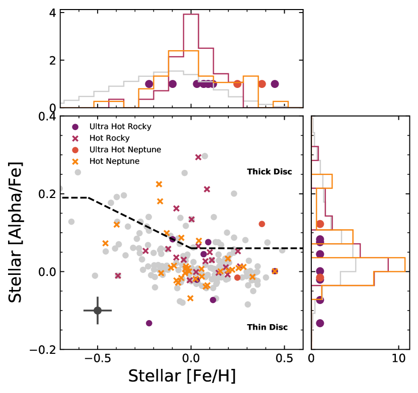
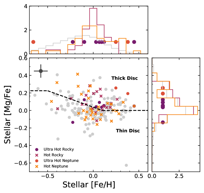
Figure 8: Left: Stellar iron abundance values are plotted against their $\alpha$ (left) and magnesium (right) abundances for our confirmed and candidate planet host stars. The dashed-lines represents the distinction between the different stellar populations of thick and thin-disc stars as shown in Adibekyan et al. (2012b) and Hayden et al. (2017) for our $\alpha$ and Mg abundances respectively. Different short (terrestrial - pink cross; Neptune - yellow cross) and ultra short (terrestrial - purple disc; Neptune - orange disc) period planet populations are highlighted within the figure. Thick disc stars are typically associated with being above the plane of the dark grey dashed line, with thin-disc stars being associated below it. Median errorbars are shown within each plot as grey markers.

Its equilibrium temperature rivals that of K2-106 b, with our derived T_eq being 2514 $\pm$ 70 K. Dorn et al. (2019) has postulated that WASP-47 e may have an exotic composition of a Ca and Al-rich interior without any atmosphere. But if there is an atmosphere, with an escape velocity of 22.44 $\pm$ 0.99 $kms^{-1}$, it may contain ionic calcium, silicon, magnesium, and maybe even aluminium with its extreme equilibrium temperature (Dorn et al., 2019). The albedo of such worlds is still a field of active research, with Kane et al. (2020) being able to constrain the geometric albedo of its sibling, WASP-47 b, to be 0.0016 but were unable to constrain WASP-47 e’s. However there was some evidence to suggest that WASP-47 e’s geometric albedo could also be as low as WASP-47 b, but a wide range of geometric albedo solutions were also found. Contrary to this, Modirrousta-Galian et al. (2021) found that high spherical albedos for super-Earths could be explained by molten Fe-rich magma oceans on the surface of ultra-short period worlds (Rouan et al., 2011).

(v) K2-131 b: Orbiting around the K dwarf K2-131 is an ultra-short period exoplanet known as K2-131 b (Dai et al., 2017). Currently a single planet system, our stellar mass and radius values of 0.75 $\pm$ 0.01R_⊙ and 0.82 $\pm$ 0.02M_⊙ are comparable to values found within the archive. Discovered in 2017, we have combined our stellar parameters and observed parameters from other surveys to revise K2-131b’s radius and mass to be 1.68 $\pm$ 0.05R_⊕ and 6.56 $\pm$ 1.07M_⊕ respectively. K2-131 b is another super-Earth predicted to host an ocean of molten lava, with a hot-dayside equilibrium temperature of 2496 $\pm$ 66 K. Its density, escape velocity and insolation flux of 7.52 $\pm$ 1.37 gcm^-3 , 22.09 $\pm$ 1.86 kms^-1 and 3865 $\pm$ 300 S_$\oplus$ respectively, is comparable to that of K2-141 b (Barragán et al., 2018). Theoretical models have predicted that K2-141 b could have an atmosphere of Na, Si and SiO₂ that is continually replenished from the up-cycling of vapourised refractory material being displaced back into its atmosphere (Nguyen et al., 2020). Such atmospheres could potentially be detected through space-based telescopes such as JWST, which will be launched later this year.

(vi) CoRoT-7 b: Whilst there have been smaller exoplanets discovered since, CoRoT-7 b (Léger et al., 2009; Queloz et al., 2009) was one of the first ultra-short period super-Earths to be discovered, the origins and evolution of which are still an active area of research (Léger et al., 2011; Winn et al., 2018; Dai et al., 2019; Lichtenberg et al., 2021). We have determined the stellar radius and mass of CoRoT-7 to be 0.84 $\pm$ 0.01R_⊙ and 0.87 $\pm$ 0.03M_⊙ respectively. Given the observed transit depths and semi-amplitudes of CoRoT-7 b found within the literature, and our derived astrophysical parameters for CoRoT-7, we have refined its planetary radius and mass to now be 1.68 $\pm$ 0.04R_⊕ and 4.94 $\pm$ 0.41M_⊕. That is, we have increased its radius and mass precision to 2.4% and 8.3% respectively, the most precise physical values for CoRoT-7 b currently available.

With these precise values, CoRoT-7 b’s radius is now large enough for an atmosphere to contribute to its overall radius (Rogers, 2015), with its density being, 5.73 $\pm$ 0.61 gcm^-3, comparable to that of Earth’s, $\rho$_$\oplus$ = 5.51 gcm^-3 (Perryman, 2018). Receiving 1682 $\pm$ 122 S_$\oplus$, CoRoT-7 b’s well-mixed and hot day-side equilibrium temperatures of 1705 K and 2027 K make it one of the cooler ultra-short period planets discussed in this section.

4.4 Chemical Abundances of Confirmed and Candidate Exoplanets

One of the biggest strengths of all-sky surveys such as GALAH is the not only access to the physical properties of these stellar hosts within our sample, but also the numerous chemical abundances that are included as well. The chemical links between stars and the planets that they host has been widely studied (Adibekyan, 2019; Fischer & Valenti, 2005; Teske et al., 2019). We are interested within our sample if there are any thick-disc hosts within our sample, and to see if there is a trend between stars that hosts close in gaseous worlds, compared to their rocky hosting counterparts.

4.4.1 Searching for thick-disc hosts within GALAH

The density and populations of stars vary significantly within the Milky Way’s disc. The thin-disc is contained within the galaxy’s innermost plane, hosting relatively young (6 Gyr), iron-rich ([Fe/H]_thin $\sim$ 0.0 dex), $\alpha$-poor ([$\alpha$/Fe]_thin $\sim$ -0.1 dex) and low total space velocity ($v_{tot}\leq$ 50 kms^-1) stars (Sharma et al., 2019; Nissen, 2004). However the thick-disc, lying in the Milky Way’s outer plane, consists of a much higher proportion of older stars, with a mean stellar age around 9.5 Gyr (Sharma et al., 2019). Not only are these stars older, but their iron abundance is lower ([Fe/H]_thick $\sim$ - 0.367 dex ), their $\alpha$-process (i.e. Mg, Si, Ca and Ti) elemental abundances are enriched ([$\alpha$/Fe]_thick $\sim$ 0.218 dex), and have faster velocities (70 $\leq v_{tot}\leq$ 200 kms^-1) compared to their thin-disc counterparts (Sharma et al., 2019; Nissen, 2004). Within the Solar neighbourhood, 1% to 12% of stars are estimated to be considered members of the Milky Way’s thick-disc (Bland-Hawthorn & Gerhard, 2016), with a few exoplanets being announced orbiting thick-disc stars (Gan et al., 2020; Weiss et al., 2021; Bouchy et al., 2010). With the above population statistics, there should be in the order of 35 – 400 exoplanet hosts from the thick-disc in which we can then better understand the underlying exoplanetary population and architectures of thick-disc planetary systems.

With this motivation, we used GALAH DR3 stellar abundances, specifically the iron and $\alpha$ abundances, along with the galactic kinematic and dynamic information within GALAH’s value added catalog, to constrain the stellar populations of known and candidate exoplanetary systems. In Figure 8 we plot the iron abundance of known confirmed and candidate systems against the stars’ $\alpha$ and magnesium abundances (a more thorough discussion between the populations outlined in the Figure is discussed in Section 4.4.2). Figure 8A shows a host star’s iron abundance against its $\alpha$ abundance, with dashed lines within the plot chemically separating stars within the thick and thin disc regions of the Milky Way as per Adibekyan et al. (2012b). We also use a one-sigma cutoff of the $\alpha$ and iron abundances from the separation line to determine the stellar populations from these chemical abundances. From these cut offs, we have 13 stars, or 5% of our host stars potentially from the thick-disc. These stars, along with their $\alpha$ and iron abundances can be found within Table 2.

Another way to determine the stellar populations of stars within the galaxy is through kinematic and dynamic data. A stars velocity towards the Galactic Centre (U), in the direction of rotation (V) and upwards from the disk (W) can be determined though large spectroscopic surveys combining astrometric data from Gaia Gaia Collaboration et al. (2020) and radial velocity data from GALAH (Buder et al., 2020; Bland-Hawthorn & Gerhard, 2016). We have used these stellar velocities from GALAH DR3 to create a Toomre diagram found in Figure 9. The Toomre diagram shows the the radial and perpendicular ($\sqrt{U_{LSR}^{2}+W_{LSR}^{2}}$) stellar velocities for all known confirmed and candidate exoplanet hosts, corrected for the Local Standard of Rest (LSR). We have included in Table 2 stars will total space velocities ($v_{tot}=\sqrt{U_{LSR}^{2}+V_{LSR}^{2}+W_{LSR}^{2}}$) greater than 70 $kms^{-1}$to bring the number of potential thick-disc host stars to 30. We can also see in the Figure, that there are stars that have chemical abundances suggesting that they are from the thick-disc, yet have stellar velocities similar to that of thin disk stars. However, past surveys have also shown that galactic thick-disc stars will often have similar kinematics to those stars found in the thin-disc (Chen et al., 2021; Kovalev et al., 2019).

We have also included in Figure 9, the stellar dynamics of our exoplanet hosts; L_z and J_R. L_z is the azimuthal angular momentum of a star and describes the amount of rotation a star’s orbit has around the Galactic centre (Trick et al., 2019; Bland-Hawthorn & Gerhard, 2016). J_R is describes the radial action of a star and can be considered a measure of a star’s orbital eccentricity (Trick et al., 2019; Bland-Hawthorn & Gerhard, 2016). Thick-disc stars would be considered to have higher J_R, as thick-disc stars have more eccentric orbits than their thin-disc counter parts (Buder et al., 2020) and have L_z values diverging away from the solar neighbourhood L_z value of 2038.3 kpc $kms^{-1}$.

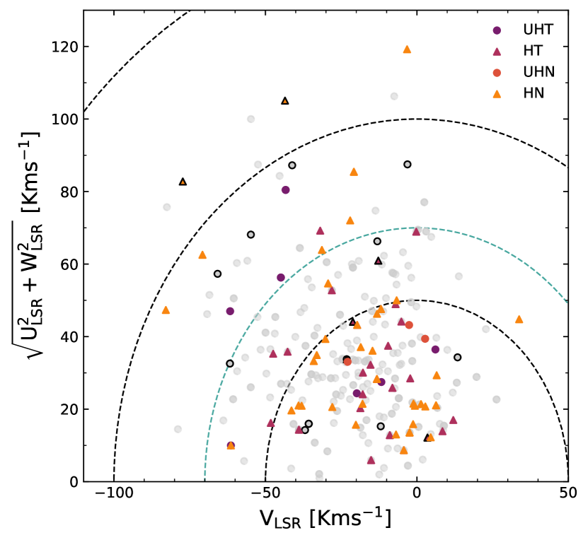
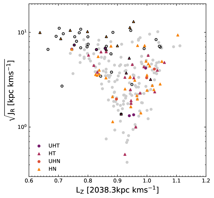
Figure 9: Left: Toomre diagram for the planet hosting and stars without planets. The red squares and blue triangles represent stars with Jupiter- and Neptune-mass planets, respectively. The magenta circles and green asterisks refer to the high-$\alpha$ metal-poor (chemically defined thick disc) and high-$\alpha$ metal-rich stars without planets, and the black dots refer to the chemically defined thin disk non-host stars. Dotted grey lines indicate total space velocities of 50, 100 and 150$kms^{-1}$ with the teal dashed-line of 70$kms^{-1}$ being our thick-thin disc kinematic cutoff line. Stars with total velocities greater than 70$kms^{-1}$  are also outlined in the right figure. Right: Stellar dynamics of our planet-hosting stars including the dynanic actions J_R and L_z. L_z of the Sun is determined to be 2038.3 kpc $kms^{-1}$(Buder et al., 2020).

Carrillo et al. (2020) collated a large chemo-kinematic database for stars being observed by TESS, and determined probable likelihoods of stars within their database to be members of the thick-disc (TD/D) as per Bensby et al. (2014). These probabilities determined by Carrillo et al. (2020) suggest that stars with a TD/D > 2 would be likely members of the thick-disc, with stars having TD/D < 0.5 being associated more with the thin-disc and stars in between these values being transitional-disc stars. We have cross-matched Carrillo et al. (2020)’s catalog, with our thirty thick-disc candidate stars, with 18 confirmed cross-matches. All of the above information can now better inform us of what stellar populations these planet hosts are likely to be a part of.

From the above information we have four stars including confirmed planet hosts NGTS-4, K2-183 and EPIC 211770696 along with the multi-planet hosting candidate star TOI-810 to be members of the thick-disc. West et al. (2019) announced the discovery of NGTS-4 b, showing that its host star’s kinematics made it a member of the thick-disc. With GALAH’s chemical abundances, [Fe/H] = -0.17  $\pm$ 0.06, [$\alpha$/Fe] = 0.22  $\pm$ 0.03, we independently confirm that NGTS-4 is indeed a member of the thick-disc. With the highest J_R within our candidates, along with a low iron abundance ([Fe/H] = -0.44  $\pm$ 0.18) and enriched $\alpha$ abundance ([$\alpha$/Fe] = 0.07  $\pm$ 0.1) we also consider candidate planet host EPIC 211064647 to also be a member of the thick disc. It is interesting to note that TOI-810 has one of the lowest J_R values within the potential thick-disc members, however has a TD/D value of 2.53. This shows that all chemo-kinematic and dynamical information needs to be considered before determining what population a star is associated with. With Carrillo et al. (2020)’s database and our results, we also consider EPIC 211800191 and EPIC 213546283 to be members of the transition area of the Milky Way. During the writing of this paper, EPIC 211770696.01 and EPIC 211978988.01 were confirmed as exoplanets and were given the designation of K2-337 b and K2-341 b respectively (de Leon et al., 2021). However, our work shows for the first time that K2-337 b has characteristics associated with being a thick-disc planetary system and K2-341 b is orbiting a star likely associated with the Milky Way’s thin disc. Due to the complex and non-linear nature that the chemical, kinematic and dynamic information that stars have with their associated stellar groups, we leave the rest to be characterised in further studies. Having a homogeneous and more inclusive sample of thick-disc stars, such as Chen et al. (2021) and others, would allow exoplanetary scientists to better probe the characteristic planetary population differences between the stellar populations, leading onto implications for astrobiology and habitability across the Milky Way (Santos et al., 2017).

Table 2: Our potential thick-disc host stars are presented in this table with their chemical, kinematic and dynamic information. The Table is sorted by the star’s radial action. TD/D probability values are taken from Carrillo et al. (2020) for stars within our sample that had matching TIC IDs.

Star name	[Fe/H]	[$\alpha$/Fe]	VSLR	$\sqrt{U_{SLR}^{2}+W_{SLR}^{2}}$	JR	LZ	TD/D
	dex	dex	$kms^{-1}$	$kms^{-1}$	kpc $kms^{-1}$	kpc $kms^{-1}$
EPIC 211064647	-0.44  $\pm$ 0.18	0.07  $\pm$ 0.1	-259.1	79.94	715.6	-91
K2-64	-0.08  $\pm$ 0.12	0.09  $\pm$ 0.07	-3.241	119.2	168.4	1935
K2-181	0.25  $\pm$ 0.07	0.01  $\pm$ 0.04	-20.8	85.45	126.2	1910	0.221
EPIC 211770696	-0.36  $\pm$ 0.09	0.2  $\pm$ 0.05	-82.53	75.71	121.8	1425	4.52
TOI-933	-0.61  $\pm$ 0.06	0.26  $\pm$ 0.03	-54.8	68.13	116.1	1573	0.291
K2-204	-0.11  $\pm$ 0.06	0.01  $\pm$ 0.02	-70.77	62.55	110.2	1500
EPIC 212624936	-0.07  $\pm$ 0.08	0.09  $\pm$ 0.05	-7.493	106.3	109.4	1916
EPIC 213546283	-0.17  $\pm$ 0.06	0.18  $\pm$ 0.02	-43.53	105.1	103.6	1619	0.545
EPIC 210961508	0.1  $\pm$ 0.12	0.1  $\pm$ 0.06	-45.32	84.32	99.61	1794
EPIC 216111905	-0.23  $\pm$ 0.12	0.17  $\pm$ 0.07	-82.87	47.34	98.95	1293
EPIC 212495601	-0.2  $\pm$ 0.09	0.05  $\pm$ 0.04	-54.8	100	97.81	1562	0.294
EPIC 201561956	-0.64  $\pm$ 0.12	0.13  $\pm$ 0.06	-69.25	46.21	93.35	1453
TOI-832	0.4  $\pm$ 0.08	-0.02  $\pm$ 0.04	-78.89	14.48	82.26	1403
K2-248	-0.13  $\pm$ 0.08	0.1  $\pm$ 0.04	-31.36	63.91	81.33	1748
TOI-348	0.08  $\pm$ 0.09	-0.01  $\pm$ 0.05	-59.44	60.31	80.61	1531	0.261
TOI-844	-0.03  $\pm$ 0.08	0.03  $\pm$ 0.04	-55.98	60.92	80.3	1622	0.18
NGTS-4	-0.17  $\pm$ 0.06	0.22  $\pm$ 0.03	-77.27	82.75	73.46	1435	103
EPIC 211800191	-0.7  $\pm$ 0.13	0.21  $\pm$ 0.06	-3.113	87.5	70.26	2090	0.577
K2-7	-0.4  $\pm$ 0.09	0.19  $\pm$ 0.05	-60.47	50.56	64.63	1544
TOI-924	-0.28  $\pm$ 0.05	0.1  $\pm$ 0.02	-52.45	87.46	56.11	1624	0.367
TOI-868	-0.1  $\pm$ 0.05	0.08  $\pm$ 0.01	-61.64	47	53.85	1528	0.0956
K2-73	0.02  $\pm$ 0.05	-0.02  $\pm$ 0.02	-22.03	72.03	51.98	1825	0.0252
TIC 287328202	-0.06  $\pm$ 0.12	0.14  $\pm$ 0.06	-41.16	87.24	50.73	1749	0.105
HATS-52	-0.31  $\pm$ 0.11	0.06  $\pm$ 0.05	2.438	77.06	48.78	2119
EPIC 211736305	0.13  $\pm$ 0.15	0.19  $\pm$ 0.08	-65.79	57.32	47.15	1572
K2-183	0.07  $\pm$ 0.11	0.04  $\pm$ 0.06	-43.32	80.45	45.97	1741	2.7
EPIC 211978988	0.02  $\pm$ 0.08	-0.0  $\pm$ 0.05	-13.67	74.74	45.32	2008	0.0737
EPIC 212646483	-0.27  $\pm$ 0.08	0.13  $\pm$ 0.04	-68.48	51.5	43.55	1348
EPIC 218901589	-0.12  $\pm$ 0.05	0.06  $\pm$ 0.02	-31.92	69.22	43.24	1748	0.033
EPIC 220674823	0.09  $\pm$ 0.09	0.08  $\pm$ 0.05	-44.9	56.29	43.21	1681	0.0579
TOI-810	-0.24  $\pm$ 0.05	0.12  $\pm$ 0.02	-38.64	64.44	11.85	1709	2.53

4.4.2 Chemical Abundance Relationships Between Short Period and Ultra-short Period Planets

There has been a great range of studies to link the chemical abundances of stars to the planets they host. The first link was discovering hot-Jupiters tending to favour iron-rich host stars (Santos et al., 2001; Fischer & Valenti, 2005; Gonzalez, 1997). Adibekyan et al. (2012a) showed that there is an overabundance of alpha-elements in short-period exoplanet hosts, in particular Neptune and super-Earth sized exoplanets, compared to stars hosting larger planets. Winn et al. (2017) showed through iron abundances of planet hosts, that there was a population difference between hot-Jupiter’s and their ultra short period counterparts, concluding that rocky USP planets might not necessarily be remnants of hot-Jovian cores. Further, Dai et al. (2019) also argued that short-period rocky worlds are more than likely exposed rocky cores of sub-Neptunes, rather than hot-Jupiters. Per the discovery of the USP TOI-1444b, Dai et al. (2021) showed that hot-Neptunes tended to favour iron-rich stars, compared to their rockier counterparts. All of the above then motivates us, with our homogenous sample to explore the abundance trends between different short-period planet types.

Firstly, we split up our sample into five different categories; Ultra Hot Rocky (USR) exoplanets (R_P < 2 R_⊕; P_p < 1 day; N = 9), Hot Rocky (HR) exoplanets (R_p < 2 R_⊕; 1 day $\leq$ P_p < 10 days; N = 36), Ultra Hot Neptune (UHN) exoplanets (2 R_⊕$\leq$ R_p < 4 R_⊕; P_p < 1 day; N = 3), Hot Neptune (HN) exoplanets ( 2 R_⊕$\leq$ R_p < 4 R_⊕; 1 day $\leq$ P_p < 10 days; N = 48), and all other candidates that fit outside of these parameters. We plot the iron abundance, against the $\alpha$-element and magnesium abundances for these populations in Figure 8. Within Figure 8A, we see a range range of iron abundances for both HN and HR worlds. Near solar values, there is a similar distribution of these two populations, however beyond [Fe/H] > 0.15, there are a greater fraction of HNs compared to their rocky counterparts. We do see a difference in the magnesium abundances however between the two populations, as HR worlds tend to favour a wider range of magnesium abundances. In contrast, HNs are seen in more magnesium poor environments peaking at near Solar values. Adibekyan et al. (2012a) showed an over-abundance of magnesium for Neptune and super-Earth hosting stars, but these two populations were entangled within the same distribution for their comparison between hot-Jupiters, thus it is difficult to compare our results with theirs in this particular case. As with Dai et al. (2021), we do see UHNs around stars enriched in iron compared to UHRs, with the one exception being the UHR exoplanet WASP-47 e, orbiting around an extremely iron-rich host ([Fe/H] = 0.45 $\pm$ 0.09). There does also seem to be a trend in UHNs being preferentially found around higher [Mg/Fe] stars compared to UHRs, but this trend for ultra-short exoplanets severely weakens out for the $\alpha$-abundance (which is a combination of Ca, Mg, Ti and Al). With an exceedingly small sample size for both ultra-short period populations (N_UHR = 9, N_UHN = 3), more data and planets are needed to confirm the existence of such trends and their implications.

Similar to Winn et al. (2017), we wanted to see if there is a difference between the populations of HRs and HNs. In our case we not only have access to [Fe/H], but we also have access to over 20 abundances, which provides a more rigorous chemical test to see if our visual discrepancy in magnesium and $\alpha$ abundances between the two populations is real or not. We perform a two-sample Kolmogorov-Smirnov test between the HN and HR populations for all GALAH abundances. The Kolmogorov-Smirnov-statistic and p-value for each element is shown in Table 3, sorted by their lowest p-value. Surprisingly, the p-value between the two populations for the magnesium abundance was 0.052, meaning that their is no statistical evidence that the magnesium abundances for the two populations are significantly different from one another. Of the 29 abundances, only three distributions had p-values smaller than 0.05, those elements being Y, Ce, and Al. We have plotted the yttrium, cerium and aluminium abundances in Figure 10.

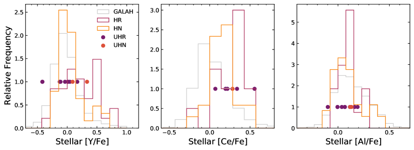
Figure 10: Chemical abundance distributions for the three elements, yttrium (Left), cerium (Middle) and aluminium (Right), that had p-values indicative of UN (pink) and HR (yellow) worlds being derived from different populations. We have included the overall GALAH abundance distributions (grey) along with the UHR (purple discs) and UHN (orange discs) for comparison as well.

The overall yttrium abundance distributions for HN and HR worlds is similar to the overall GALAH distribution, however we do see a trend where by more HR exoplanets are found around a broader range of [Y/Fe] values. We also see a higher fraction of HR planets orbiting stars enriched in yttrium ([Y/Fe] > 0.2) compared to their gaseous counterparts. As yttrium is known as a “chemical-clock" element, whereby stars enriched in yttrium are typically younger, we see this trend as a possibility that HR planets tend to favour younger stars (Titarenko et al., 2019; Slumstrup et al., 2017). However, we also see a trend whereby HR worlds tend to favour magnesium-enriched stars. Magnesium is also a “chemical-clock" element, but enhanced magnesium abundances are often a reflection of orbiting around older stars (Titarenko et al., 2019). Thus, this positive correlation between magnesium and yttrium needs further investigation to determine as to why HR planets tend to favour stars enriched in both of these elements. Cerium has similar trends, with HR stars being enriched with Ce compared to HN hosting stars. However, both HN and HR [Ce/Fe] abundances peak super-Solar, compared to the Solar-like abundance peak for the overall GALAH sample, with the interpretation to this distribution remaining an interesting development for future work.

Overall, there does not seem to be a statistical difference between the chemical properties of stars that host HNs and those that host HRs. Thus, following the conclusions of Dai et al. (2021) and Winn et al. (2017), our more robust chemical abundance results show that there is a possibility that short-period rocky worlds might be the remnant cores of hotter-gaseous Neptune worlds. The reason being is that there are only three of the 29 elemental abundances that had KS statistics significant enough to show that HRs and HNs come from different populations. Even with these three elements, the smallest p-value of 0.01, along with a relatively small sample size of our HRs and HNs, there is still more research to be done to determine the similarities in these populations, and thus determine the origins and evolution of short-period exoplanets.

Table 3: Our two-sample Kolmogorov-Smirnov test results between our Hot Neptune and Hot Rocky planet samples for each GALAH abundance.

Element	D-statistic	p-value
Y	0.364	0.01
Ce	0.476	0.024
Al	0.303	0.037
Mg	0.299	0.052
Na	0.25	0.132
Cr	0.238	0.169
Ba	0.236	0.176
$\alpha$	0.217	0.254
Cu	0.212	0.275
K	0.21	0.302
Mo	0.625	0.303
Zr	0.326	0.311
C	0.571	0.318
O	0.235	0.323
La	0.367	0.357
Si	0.2	0.357
Mn	0.19	0.39
Rb	0.889	0.4
Sm	0.667	0.4
Sc	0.183	0.46
Li	0.333	0.5
Ca	0.166	0.571
Co	0.201	0.573
Fe	0.16	0.622
Zn	0.16	0.629
Ti	0.147	0.707
V	0.159	0.821
Ni	0.11	0.945
Nd	0.667	1.0

4.5 Assessing the radius valley and super-Earth desert

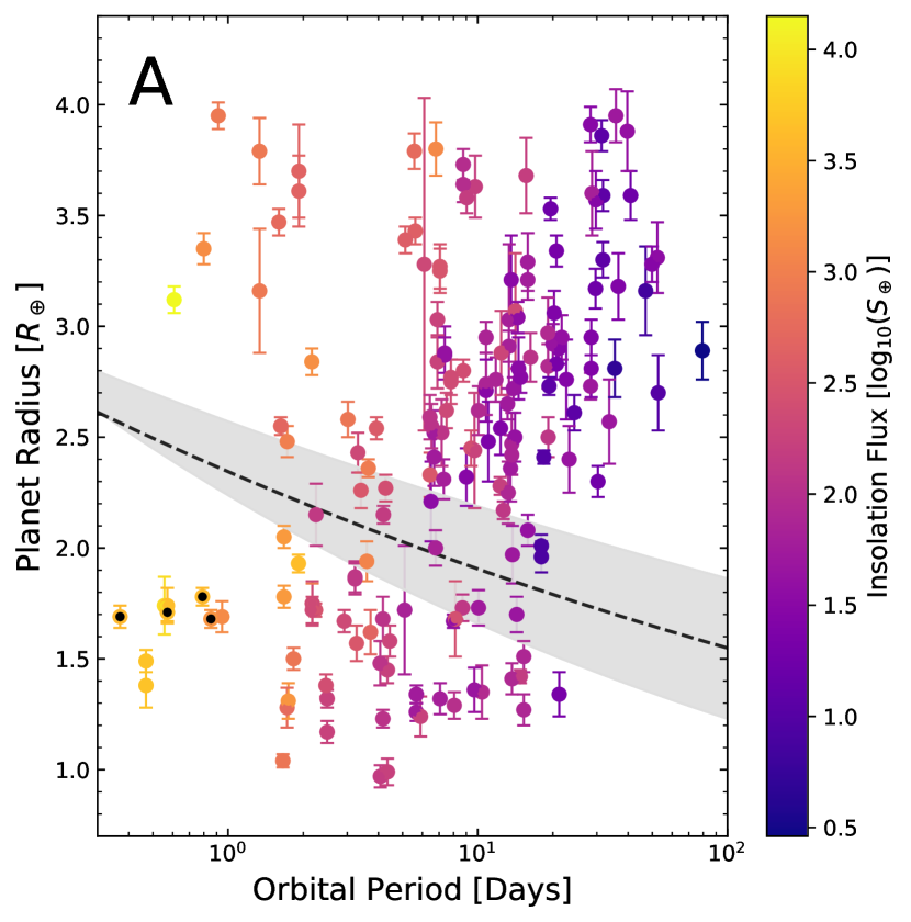
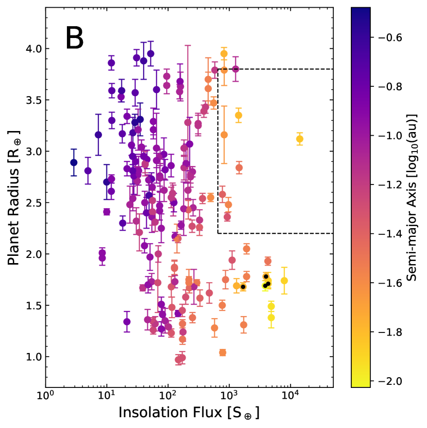
Figure 11: Left: Our confirmed and candidate exoplanet planetary radius values are plotted against their orbital periods, each being coloured by their insolation flux values. The dashed line and shaded region around it, indicates the slope and error in the radius valley as noted by Van Eylen et al. (2018) Right: Planet and candidate radius values are plotted against their incident flux, coloured by their semi-major axis values. The dashed lines enclose the hot Super-Earth desert noted by Lundkvist et al. (2016). Our four ultra-short period super-Earths are depicted in each plot by black dots.

Because we have four ultra-short period exoplanets within our sample straddling the super-Earth radius gap, we show in Figure 11a their location in the so-called two-dimensional radius gap, i.e. the planetary radius compared to the orbital period (Fulton et al., 2017; Van Eylen et al., 2018). None of the ultra-short period super-Earths within our sample lie within the photoevaporation valley, the grey dashed line within the Figure 11a, all below this line. Nor do any of these ultra-short period have periods smaller than the expected Roche limits of their host stars (Rappaport et al., 2013). They do however has orbits that are smaller than the dust sublimation radius of their host stars (Isella et al., 2006), meaning that in-situ formation of these exoplanets is unlikely. There is only one confirmed-exoplanet that lies within 1-sigma of the line proposed by Van Eylen et al. (2018), that being K2-247 b (P: 2.25 d, R_p: 2.15 $\pm$ 0.14 R_⊕) (Livingston et al., 2018a).

We show also in Figure 11 the insolation flux of confirmed and candidate exoplanets compared to their estimated radii; the dashed lines enclose a region of parameter space known as the Neptunian desert, proposed by (Lundkvist et al., 2016). This Neptunian desert is a region of flux-radius phase space where super-Earths are less common, explained by evaporation of volatile elements. The sub-Neptune NGTS-4 b (S_eff: 824 $\pm$ 62 S_$\oplus$, R_p: 3.16 $\pm$ 0.29R_⊕) is the only confirmed exoplanet within this region (West et al., 2019) with two TOIs, 1926.01 and 1948.01, also being contained within the Neptunian desert.

As mentioned previously, the origin of ultra-short period super-Earths remains an active field of science (Wagner et al., 2012; Lundkvist et al., 2016; Nguyen et al., 2020; Spaargaren et al., 2020). The elemental abundances of refractory elements, such as Mg, Si, Fe and molar ratios of such elements can help constrain the interiors of rocky worlds (Unterborn et al., 2016; Seager et al., 2007; Valencia et al., 2006). Modelling the interiors of ultra-short period can help determine if these worlds are likely remnants of Jovian cores, or super-Earths that have migrated inwards to their current positions (Mocquet et al., 2014; Benz et al., 2007). 44% of ultra-short period super-Earths discovered are enriched with iron, with exoplanet candidate KOI 1843.03 predicted to have a core-mass fraction as high as mercury’s. However, there seems to be no trend between a rocky planet’s core-mass fraction and its received flux values (Price & Rogers, 2020). Mg/Si and Fe/Si ratios from GALAH DR3 could be used to further constrain the chemical and geological composition of these super-Earths using models such as Dorn et al. (2015, 2017); Wang et al. (2019) and Unterborn et al. (2018b). But this is outside the scope of this paper and is left for further future investigation.

5 Conclusion

The wealth of astronomical data in large galactic archaeology surveys like GALAH can be used in numerous astrophysical fields, including exoplanetary science. We have cross-matched GALAH’s latest release with the latest astrometric data from Gaia EDR3 to determine the physical parameters of 279 confirmed and candidate exoplanet hosting stars. With these new stellar parameters and combining planetary observables from transit photometry and Doppler spectroscopy where applicable, we have determined and refined the physical characteristics of 105 confirmed exoplanets, 146 K2 candidates, 95 TOIs and 52 CTOIs, along with analysing the chemical abundances of these host stars. From our study we have uncovered:

• 30 CTOI and K2 candidates have radii larger than our planetary limit of R_P $<$ 2 R_J, meaning that these candidates would be more akin to brown-dwarfs or stellar companions. TOIs 147.01, 565.01, 959.01, 1072.01 and 2391.01 are also too large to be planetary in nature.
  

• For the majority of our candidates, their host star’s $v\sin{i}$values are above 5$kms^{-1}$, with predicted RV signals being less than 5$ms^{-1}$. We then predict that it will be difficult, with current methodology, to obtain mass confirmations for most of the smaller planet candidates orbiting stars found within our sample. In the extreme cases for smaller planets orbiting rapid-rotating stars it will be highly improbable to derive their mass measurements, with TOI-1219.01 needing over 14,000 RV measurements to confirm its mass from a typical modern spectrograph.
  

• Out of the homogeneous data set of 105 exoplanets with new planetary parameters, we have updated parameters for five ultra-short period super-Earths – K2-106 b, K2-216 b, WASP-47 e, K2-131 b and CoRoT- 7 b – which make up 28% of all such planets with known mass and radius values. In particular, our refined radius and mass values for WASP-47 e, K2-106 b and CoRoT-7 b have uncertainties smaller than 2.3% and 8.5%, respectively. From these refinements, K2-106 b’s equilibrium temperature of 2570 K far exceeds the condensation temperature of most refractory elements, making it the hottest super-Earth to date. With our mass and radius measurements of CoRoT-7 b, 1.68 $\pm$ 0.04R_⊕ and 4.94 $\pm$ 0.41M_⊕ respectively, its radius is now large enough for an atmosphere to contribute to its overall radius and now straddles the super-Earth radius gap.
  

• Through stellar chemo-kinematic and dynamical data, we announce that three confirmed planet hosts, including NGTS-4, K2-183 and K2-337 along with candidate host stars TOI-810 and EPIC 211064647 to be members of the Milky Way’s thick disc. By knowing more thick-disc hosts, we will be able to better determine the statistics of planetary architectures across stellar populations and determine the habitability of systems across the galaxy.
  

• With GALAH chemical abundances, we have shown that there does not seem to be a statistical difference between the chemical properties of stars that host Hot Neptunes and those that host Hot Rocky exoplanets. Thus, there is a possibility that short-period rocky worlds might be the remnant cores of hotter-gaseous Neptune-sized worlds.

Software

AstroPy (Astropy Collaboration et al., 2013), Astroquery (Ginsburg et al., 2019), Isochrones (Morton, 2015), Matplotlib (Hunter, 2007), MultiNest (Feroz et al., 2019; Feroz et al., 2009; Feroz & Hobson, 2008), Multiprocessing (McKerns et al., 2012), NumPy (Oliphant, 2006; van der Walt et al., 2011), Pandas (McKinney et al., 2010), SciPy (Virtanen et al., 2020)

Data Availability

The data underlying this article are available in the article and in its online supplementary material.

Appendix A Data Tables

Table 4: Our stellar parameters for confirmed and candidate exoplanet hosting stars. The full table of which can be found on the online version of this paper.

TIC ID	2MASS ID	GAIA DR3 ID	RA	Dec	Teff	log $g$	[Fe/H]	[$\alpha$/Fe]	[M/H]	$\cdots$
			[deg]	[deg]	[K]	[cgs]	[dex]	[dex]	[dex]	$\cdots$
355703913	00030587-6228096	4904523077718046720	0.7745$\pm$0.0099	-62.4693$\pm$0.0096	5451$\pm$112	4.50$\pm$0.19	0.23$\pm$0.10	0.05$\pm$0.06	0.30$\pm$0.14	$\cdots$
70785910	00062006-3020105	2320600658577841536	1.5836$\pm$0.0152	-30.3364$\pm$0.0115	5819$\pm$96	4.09$\pm$0.19	0.08$\pm$0.09	-0.01$\pm$0.05	0.06$\pm$0.12	$\cdots$
201256771	00071640-5827263	4918333184280735232	1.8187$\pm$0.0083	-58.4573$\pm$0.0084	4960$\pm$81	3.42$\pm$0.18	-0.34$\pm$0.05	0.19$\pm$0.02	-0.04$\pm$0.06	$\cdots$
328066864	00392335+0443037	2554244130700741504	9.8475$\pm$0.0148	4.7178$\pm$0.0077	4742$\pm$123	4.59$\pm$0.19	-0.12$\pm$0.12	0.06$\pm$0.08	-0.04$\pm$0.17	$\cdots$
299897516	00403884-6052497	4903399170675741568	10.1621$\pm$0.0099	-60.8804$\pm$0.0092	5417$\pm$98	3.86$\pm$0.18	-0.83$\pm$0.09	0.26$\pm$0.05	-0.42$\pm$0.12	$\cdots$
418761354	00455526+0620490	2556231154370582400	11.4802$\pm$0.0200	6.3470$\pm$0.0111	4602$\pm$88	4.61$\pm$0.18	-0.04$\pm$0.07	0.03$\pm$0.03	0.01$\pm$0.09	$\cdots$
234504626	00474568-6225232	4902237021244807296	11.9408$\pm$0.0091	-62.4232$\pm$0.0091	5001$\pm$90	4.55$\pm$0.18	0.18$\pm$0.07	0.03$\pm$0.03	0.23$\pm$0.09	$\cdots$
257394133	00485666+0524595	2552929320952237952	12.2361$\pm$0.0169	5.4164$\pm$0.0086	5617$\pm$96	4.32$\pm$0.19	0.27$\pm$0.08	-0.02$\pm$0.04	0.25$\pm$0.10	$\cdots$
257218673	00490407+0215596	2549922465888108032	12.2670$\pm$0.0146	2.2666$\pm$0.0080	5579$\pm$93	4.06$\pm$0.18	0.21$\pm$0.08	0.04$\pm$0.04	0.27$\pm$0.10	$\cdots$
405336406	00493540+1001123	2582183683235097728	12.3975$\pm$0.0185	10.0200$\pm$0.0142	4490$\pm$76	1.67$\pm$0.25	-0.74$\pm$0.05	0.20$\pm$0.01	-0.43$\pm$0.05	$\cdots$
266012991	00510476+0931003	2581918597853527424	12.7700$\pm$0.0204	9.5168$\pm$0.0144	5554$\pm$77	4.38$\pm$0.18	-0.02$\pm$0.05	0.04$\pm$0.02	0.04$\pm$0.06	$\cdots$
333605244	00510570-0111452	2535901287452166400	12.7737$\pm$0.0167	-1.1959$\pm$0.0089	4975$\pm$125	4.59$\pm$0.19	0.04$\pm$0.11	0.07$\pm$0.06	0.14$\pm$0.14	$\cdots$
257434940	00511854+0520004	2552891834477747200	12.8273$\pm$0.0152	5.3334$\pm$0.0093	5254$\pm$98	3.91$\pm$0.19	-0.13$\pm$0.08	0.13$\pm$0.05	0.06$\pm$0.11	$\cdots$
266015990	00521914+1047409	2582617711154563968	13.0800$\pm$0.0146	10.7947$\pm$0.0105	5499$\pm$104	4.40$\pm$0.19	0.09$\pm$0.09	0.08$\pm$0.05	0.21$\pm$0.12	$\cdots$
257435562	00523368+0330277	2551651031310145024	13.1404$\pm$0.0162	3.5078$\pm$0.0090	5750$\pm$88	4.21$\pm$0.18	0.10$\pm$0.07	0.05$\pm$0.03	0.18$\pm$0.09	$\cdots$
266017624	00524666+0941345	2581916673708201216	13.1944$\pm$0.0163	9.6929$\pm$0.0129	5014$\pm$91	4.54$\pm$0.19	0.33$\pm$0.07	-0.01$\pm$0.04	0.31$\pm$0.09	$\cdots$
344586726	00530642+0606009	2553369877222007168	13.2768$\pm$0.0152	6.1002$\pm$0.0108	4935$\pm$116	4.61$\pm$0.19	-0.05$\pm$0.10	-0.02$\pm$0.06	-0.07$\pm$0.14	$\cdots$
266030611	00534179+1002417	2581964605543263104	13.4241$\pm$0.0130	10.0448$\pm$0.0107	5652$\pm$88	4.44$\pm$0.18	0.35$\pm$0.07	-0.00$\pm$0.03	0.35$\pm$0.09	$\cdots$
$\cdots$	$\cdots$	$\cdots$	$\cdots$	$\cdots$	$\cdots$	$\cdots$	$\cdots$	$\cdots$	$\cdots$	$\cdots$
Rs	Ms	Ls	Age	RV	vsini	HZ1	HZ2	HZ3	HZ4	HZ5
[R$\odot$]	[M⊙]	[L$\odot$]	[log10(Gyr)]	[kms-1]	[kms-1]	[au]	[au]	[au]	[au]	[au]
0.925$\pm$0.015	0.977$\pm$0.040	0.677$\pm$0.060	9.526$\pm$0.424	17.286$\pm$0.096	5.168$\pm$2.488	0.626	0.823	0.828	1.429	1.495
1.610$\pm$0.033	1.106$\pm$0.065	2.660$\pm$0.208	9.851$\pm$0.130	31.222$\pm$0.123	5.488$\pm$2.350	1.222	1.597	1.617	2.745	2.871
3.233$\pm$0.059	1.220$\pm$0.098	5.664$\pm$0.425	9.693$\pm$0.130	-11.577$\pm$0.071	6.509$\pm$2.133	1.845	2.442	2.441	4.314	4.513
0.727$\pm$0.011	0.761$\pm$0.025	0.240$\pm$0.026	9.805$\pm$0.398	-2.143$\pm$0.081	6.950$\pm$2.492	0.382	0.507	0.506	0.904	0.946
1.765$\pm$0.036	0.928$\pm$0.037	2.400$\pm$0.200	10.041$\pm$0.056	1.605$\pm$0.117	9.993$\pm$2.320	1.180	1.553	1.561	2.699	2.823
0.688$\pm$0.010	0.723$\pm$0.019	0.190$\pm$0.016	9.719$\pm$0.419	-26.481$\pm$0.081	6.666$\pm$2.247	0.342	0.454	0.453	0.814	0.853
0.801$\pm$0.011	0.865$\pm$0.024	0.359$\pm$0.028	9.533$\pm$0.425	20.991$\pm$0.073	6.239$\pm$2.250	0.464	0.614	0.614	1.082	1.132
1.167$\pm$0.027	1.019$\pm$0.042	1.214$\pm$0.100	9.912$\pm$0.128	-4.166$\pm$0.104	6.379$\pm$2.301	0.832	1.092	1.101	1.887	1.973
1.602$\pm$0.035	1.078$\pm$0.054	2.228$\pm$0.178	9.952$\pm$0.188	4.115$\pm$0.114	7.170$\pm$2.284	1.129	1.482	1.494	2.564	2.681
24.617$\pm$1.181	1.212$\pm$0.296	220.397$\pm$25.991	9.593$\pm$0.280	-148.747$\pm$0.085	7.090$\pm$2.096	11.700	15.531	15.481	27.974	29.309
1.010$\pm$0.017	0.929$\pm$0.029	0.868$\pm$0.057	9.951$\pm$0.124	13.396$\pm$0.082	4.899$\pm$2.143	0.706	0.927	0.934	1.604	1.678
0.767$\pm$0.011	0.825$\pm$0.025	0.323$\pm$0.034	9.522$\pm$0.449	18.833$\pm$0.104	3.666$\pm$2.651	0.440	0.583	0.582	1.028	1.076
1.794$\pm$0.039	1.003$\pm$0.035	2.195$\pm$0.190	10.033$\pm$0.081	11.729$\pm$0.115	10.051$\pm$2.262	1.135	1.498	1.502	2.618	2.738
0.969$\pm$0.017	0.969$\pm$0.045	0.769$\pm$0.064	9.756$\pm$0.321	-16.011$\pm$0.096	6.027$\pm$2.367	0.665	0.875	0.880	1.517	1.586
1.337$\pm$0.024	1.086$\pm$0.043	1.749$\pm$0.124	9.837$\pm$0.129	-6.373$\pm$0.109	5.812$\pm$2.260	0.994	1.300	1.315	2.239	2.342
0.817$\pm$0.013	0.871$\pm$0.028	0.378$\pm$0.030	9.677$\pm$0.407	-5.682$\pm$0.068	6.797$\pm$2.251	0.475	0.629	0.629	1.109	1.160
0.728$\pm$0.012	0.773$\pm$0.025	0.282$\pm$0.028	9.655$\pm$0.444	8.326$\pm$0.083	6.188$\pm$2.447	0.412	0.545	0.545	0.964	1.009
1.037$\pm$0.019	1.062$\pm$0.042	0.982$\pm$0.071	9.527$\pm$0.378	-9.459$\pm$0.098	7.432$\pm$2.237	0.747	0.980	0.989	1.692	1.769
$\cdots$	$\cdots$	$\cdots$	$\cdots$	$\cdots$	$\cdots$	$\cdots$	$\cdots$	$\cdots$	$\cdots$	$\cdots$

Table 5: Our refined confirmed and candidate exoplanet parameters. The full table of which can be found on the online version of this paper.

TIC ID	Candidate	Period	Semi-major axis	Rp/R*	au/R*	Transit Depth	Inclination	Eccentricity	Kamp	$\cdots$
	Name	[Days]	[au]			[%]	[deg]		[ms-2]	$\cdots$
677945	K2-128 b	5.675729$\pm$0.0001680	0.0559$\pm$0.0004	0.01709$\pm$0.00059	17.8385$\pm$0.268	0.029239$\pm$0.001693	88.331$\pm$0.574	0.23$\pm$0.221	$\cdots$	$\cdots$
677945	EPIC 212686205.01	5.67556$\pm$0.0002900	0.0559$\pm$0.0004	0.01822$\pm$0.00058	17.8382$\pm$0.268	0.0332$\pm$0.001700	$\cdots$	$\cdots$	$\cdots$	$\cdots$
678699	EPIC 212560683.01	13.7043$\pm$0.0037000	0.1134$\pm$0.0012	0.01257$\pm$0.0006	23.7383$\pm$0.463	0.0158$\pm$0.001300	$\cdots$	$\cdots$	$\cdots$	$\cdots$
706595	K2-194 b	39.72342$\pm$0.0031880	0.2358$\pm$0.0034	0.02562$\pm$0.00128	36.5615$\pm$0.898	0.06572$\pm$0.005381	89.065$\pm$0.46	$\cdots$	$\cdots$	$\cdots$
706595	EPIC 212672300.01	39.703624$\pm$0.0021210	0.2358$\pm$0.0034	0.02721$\pm$0.00093	36.5523$\pm$0.897	0.0741$\pm$0.002800	$\cdots$	$\cdots$	$\cdots$	$\cdots$
707724	EPIC 212585579.01	3.021889$\pm$0.0000460	0.0411$\pm$0.0007	0.03443$\pm$0.00114	7.8281$\pm$0.188	0.1186$\pm$0.004500	$\cdots$	$\cdots$	$\cdots$	$\cdots$
743782	EPIC 212652418.01	19.1324$\pm$0.0031010	0.1416$\pm$0.0024	0.01912$\pm$0.00075	22.5198$\pm$0.579	0.0366$\pm$0.002000	$\cdots$	$\cdots$	$\cdots$	$\cdots$
771548	EPIC 212587672.01	23.231764$\pm$0.0008410	0.1579$\pm$0.0025	0.02175$\pm$0.00135	33.5908$\pm$0.802	0.047326$\pm$0.005322	89.421$\pm$0.422	$\cdots$	$\cdots$	$\cdots$
771548	EPIC 212587672.02	15.2841$\pm$0.0020000	0.1195$\pm$0.0019	0.01367$\pm$0.00066	25.4093$\pm$0.607	0.0187$\pm$0.001500	$\cdots$	$\cdots$	$\cdots$	$\cdots$
771548	EPIC 212587672 b	15.2841$\pm$0.0017600	0.1195$\pm$0.0019	0.01152$\pm$0.00065	25.4108$\pm$0.606	0.01328$\pm$0.001324	$\cdots$	$\cdots$	$\cdots$	$\cdots$
1103432	565.01	3.727891$\pm$0.0004550	0.0496$\pm$0.001	0.13363$\pm$0.00451	6.2069$\pm$0.178	19.571261$\pm$0.548862	$\cdots$	$\cdots$	$\cdots$	$\cdots$
2621212	K2-199 c	7.374442$\pm$0.0000660	0.0663$\pm$0.0006	0.03868$\pm$0.0012	20.9489$\pm$0.324	0.149668$\pm$0.007299	88.893$\pm$0.557	$\cdots$	$\cdots$	$\cdots$
2621212	K2-199 b	3.225392$\pm$0.0000320	0.0382$\pm$0.0004	0.02522$\pm$0.00089	12.0707$\pm$0.187	0.063616$\pm$0.003787	87.182$\pm$1.475	$\cdots$	$\cdots$	$\cdots$
2621212	EPIC 212779596.01	3.225349$\pm$0.0000430	0.0382$\pm$0.0004	0.02506$\pm$0.001	12.0704$\pm$0.187	0.062827$\pm$0.004389	$\cdots$	$\cdots$	$\cdots$	$\cdots$
2621212	EPIC 212779596.02	7.374284$\pm$0.0001100	0.0663$\pm$0.0006	0.03876$\pm$0.00161	20.9486$\pm$0.324	0.150314$\pm$0.011041	$\cdots$	$\cdots$	$\cdots$	$\cdots$
2670610	EPIC 213546283.01	9.770225$\pm$0.0001750	0.0898$\pm$0.0012	0.02896$\pm$0.00123	16.8145$\pm$0.375	0.083943$\pm$0.005663	88.885$\pm$0.815	$\cdots$	$\cdots$	$\cdots$
2712931	EPIC 212645891.01	0.328227$\pm$0.0000010	0.0092$\pm$0.0002	0.04742$\pm$0.00135	1.7434$\pm$0.048	0.224802$\pm$0.001692	41.646$\pm$5.432	$\cdots$	$\cdots$	$\cdots$
2764004	EPIC 212624936.01	11.81387$\pm$0.0008500	0.0994$\pm$0.0015	0.02686$\pm$0.00108	22.7423$\pm$0.555	0.0722$\pm$0.004200	$\cdots$	$\cdots$	$\cdots$	$\cdots$
$\cdots$	$\cdots$	$\cdots$	$\cdots$	$\cdots$	$\cdots$	$\cdots$	$\cdots$	$\cdots$	$\cdots$	$\cdots$
Rp	Mp	Flagmass	$\rho$p	Seff	Teq WM	Teq HD	gp	$v_{e}$	Flagcat
R⊕	M⊕		gcm-3	S$\oplus$	[K]	[K]	[ms-2]	[ms-1]
1.26$\pm$0.04	$\cdots$	$\cdots$	$\cdots$	57.26$\pm$4.49	732$\pm$19	871$\pm$23	$\cdots$	$\cdots$	EXO
1.34$\pm$0.04	$\cdots$	$\cdots$	$\cdots$	57.26$\pm$4.48	732$\pm$19	871$\pm$23	$\cdots$	$\cdots$	K2
1.41$\pm$0.07	$\cdots$	$\cdots$	$\cdots$	81.14$\pm$5.28	799$\pm$19	950$\pm$23	$\cdots$	$\cdots$	K2
3.88$\pm$0.18	$\cdots$	$\cdots$	$\cdots$	39.93$\pm$3.14	687$\pm$15	817$\pm$18	$\cdots$	$\cdots$	EXO
4.12$\pm$0.12	$\cdots$	$\cdots$	$\cdots$	39.95$\pm$3.14	630$\pm$30	749$\pm$35	$\cdots$	$\cdots$	K2
4.24$\pm$0.12	$\cdots$	$\cdots$	$\cdots$	797.66$\pm$62.96	1331$\pm$63	1583$\pm$75	$\cdots$	$\cdots$	K2
2.82$\pm$0.1	$\cdots$	$\cdots$	$\cdots$	89.55$\pm$7.88	840$\pm$20	999$\pm$24	$\cdots$	$\cdots$	K2
2.4$\pm$0.15	$\cdots$	$\cdots$	$\cdots$	44.41$\pm$3.51	705$\pm$16	839$\pm$19	$\cdots$	$\cdots$	K2
1.51$\pm$0.07	$\cdots$	$\cdots$	$\cdots$	77.63$\pm$6.14	790$\pm$21	940$\pm$25	$\cdots$	$\cdots$	K2
1.27$\pm$0.07	$\cdots$	$\cdots$	$\cdots$	77.63$\pm$6.14	790$\pm$21	940$\pm$25	$\cdots$	$\cdots$	EXO
25.07$\pm$0.65	$\cdots$	$\cdots$	$\cdots$	1429.21$\pm$119.76	1420$\pm$84	1689$\pm$99	$\cdots$	$\cdots$	TOI
2.87$\pm$0.08	$\cdots$	$\cdots$	$\cdots$	42.3$\pm$3.22	697$\pm$15	828$\pm$18	$\cdots$	$\cdots$	EXO
1.87$\pm$0.07	$\cdots$	$\cdots$	$\cdots$	127.37$\pm$9.71	894$\pm$23	1063$\pm$28	$\cdots$	$\cdots$	EXO
1.86$\pm$0.07	$\cdots$	$\cdots$	$\cdots$	127.39$\pm$9.71	894$\pm$23	1064$\pm$28	$\cdots$	$\cdots$	K2
2.88$\pm$0.12	$\cdots$	$\cdots$	$\cdots$	42.29$\pm$3.22	697$\pm$15	828$\pm$18	$\cdots$	$\cdots$	K2
3.63$\pm$0.14	$\cdots$	$\cdots$	$\cdots$	159.39$\pm$11.64	971$\pm$20	1154$\pm$24	$\cdots$	$\cdots$	K2
5.87$\pm$0.12	$\cdots$	$\cdots$	$\cdots$	13416.93$\pm$1670.66	2692$\pm$143	3201$\pm$171	$\cdots$	$\cdots$	K2
2.75$\pm$0.1	$\cdots$	$\cdots$	$\cdots$	73.34$\pm$6.44	799$\pm$19	951$\pm$23	$\cdots$	$\cdots$	K2
$\cdots$	$\cdots$	$\cdots$	$\cdots$	$\cdots$	$\cdots$	$\cdots$	$\cdots$	$\cdots$	$\cdots$

References

- Addison et al. (2021) Addison B. C., et al., 2021, MNRAS, 502, 3704
- Adibekyan (2019) Adibekyan V., 2019, Geosciences, 9, 105
- Adibekyan et al. (2012a) Adibekyan V. Z., et al., 2012a, A&A, 543, A89
- Adibekyan et al. (2012b) Adibekyan V. Z., Sousa S. G., Santos N. C., Delgado Mena E., González Hernández J. I., Israelian G., Mayor M., Khachatryan G., 2012b, A&A, 545, A32
- Astropy Collaboration et al. (2013) Astropy Collaboration et al., 2013, A&A, 558, A33
- Bailes et al. (2011) Bailes M., et al., 2011, Science, 333, 1717
- Barragán et al. (2018) Barragán O., et al., 2018, A&A, 612, A95
- Barros et al. (2016) Barros S. C. C., Demangeon O., Deleuil M., 2016, A&A, 594, A100
- Batalha et al. (2013) Batalha N. M., et al., 2013, The Astrophysical Journal Supplement Series, 204, 24
- Becker et al. (2015) Becker J. C., Vanderburg A., Adams F. C., Rappaport S. A., Schwengeler H. M., 2015, ApJ, 812, L18
- Bensby et al. (2014) Bensby T., Feltzing S., Oey M. S., 2014, A&A, 562, A71
- Benz et al. (2007) Benz W., Anic A., Horner J., Whitby J. A., 2007, Space Sci. Rev., 132, 189
- Bitsch & Battistini (2020) Bitsch B., Battistini C., 2020, A&A, 633, A10
- Bland-Hawthorn & Gerhard (2016) Bland-Hawthorn J., Gerhard O., 2016, ARA&A, 54, 529
- Bonomo et al. (2019) Bonomo A. S., et al., 2019, Nature Astronomy, 3, 416
- Boss (2001) Boss A. P., 2001, ApJ, 551, L167
- Bouchy et al. (2010) Bouchy F., et al., 2010, A&A, 519, A98
- Brucalassi et al. (2017) Brucalassi A., et al., 2017, A&A, 603, A85
- Buder et al. (2018) Buder S., et al., 2018, MNRAS, 478, 4513
- Buder et al. (2020) Buder S., et al., 2020, arXiv e-prints, p. arXiv:2011.02505
- Butler et al. (1996) Butler R. P., Marcy G. W., Williams E., McCarthy C., Dosanjh P., Vogt S. S., 1996, PASP, 108, 500
- Carrillo et al. (2020) Carrillo A., Hawkins K., Bowler B. P., Cochran W., Vanderburg A., 2020, MNRAS, 491, 4365
- Chen & Kipping (2017) Chen J., Kipping D., 2017, ApJ, 834, 17
- Chen et al. (2021) Chen D.-C., et al., 2021, ApJ, 909, 115
- Choi et al. (2016) Choi J., Dotter A., Conroy C., Cantiello M., Paxton B., Johnson B. D., 2016, ApJ, 823, 102
- Clark et al. (2020) Clark J. T., et al., 2020, arXiv e-prints, p. arXiv:2008.05372
- Cui et al. (2012) Cui X.-Q., et al., 2012, Research in Astronomy and Astrophysics, 12, 1197
- Dai et al. (2015) Dai F., et al., 2015, ApJ, 813, L9
- Dai et al. (2017) Dai F., et al., 2017, AJ, 154, 226
- Dai et al. (2019) Dai F., Masuda K., Winn J. N., Zeng L., 2019, ApJ, 883, 79
- Dai et al. (2021) Dai F., et al., 2021, AJ, 162, 62
- De Silva et al. (2015) De Silva G. M., et al., 2015, MNRAS, 449, 2604
- Deleuil et al. (2008) Deleuil M., et al., 2008, A&A, 491, 889
- Dorn et al. (2015) Dorn C., Khan A., Heng K., Connolly J. A. D., Alibert Y., Benz W., Tackley P., 2015, A&A, 577, A83
- Dorn et al. (2017) Dorn C., Venturini J., Khan A., Heng K., Alibert Y., Helled R., Rivoldini A., Benz W., 2017, A&A, 597, A37
- Dorn et al. (2019) Dorn C., Harrison J. H. D., Bonsor A., Hands T. O., 2019, MNRAS, 484, 712
- Dragomir et al. (2019) Dragomir D., et al., 2019, ApJ, 875, L7
- Dressing & Charbonneau (2013) Dressing C. D., Charbonneau D., 2013, ApJ, 767, 95
- Dressing & Charbonneau (2015) Dressing C. D., Charbonneau D., 2015, ApJ, 807, 45
- Feroz & Hobson (2008) Feroz F., Hobson M. P., 2008, MNRAS, 384, 449
- Feroz et al. (2009) Feroz F., Hobson M. P., Bridges M., 2009, MNRAS, 398, 1601
- Feroz et al. (2019) Feroz F., Hobson M. P., Cameron E., Pettitt A. N., 2019, The Open Journal of Astrophysics, 2, 10
- Fischer & Valenti (2005) Fischer D. A., Valenti J., 2005, ApJ, 622, 1102
- Fulton et al. (2017) Fulton B. J., et al., 2017, AJ, 154, 109
- Gaia Collaboration et al. (2018) Gaia Collaboration et al., 2018, A&A, 616, A1
- Gaia Collaboration et al. (2020) Gaia Collaboration Brown A. G. A., Vallenari A., Prusti T., de Bruijne J. H. J., Babusiaux C., Biermann M., 2020, arXiv e-prints, p. arXiv:2012.01533
- Gan et al. (2020) Gan T., et al., 2020, AJ, 159, 160
- Gilmore et al. (2012) Gilmore G., et al., 2012, The Messenger, 147, 25
- Ginsburg et al. (2019) Ginsburg A., et al., 2019, AJ, 157, 98
- Gonzalez (1997) Gonzalez G., 1997, MNRAS, 285, 403
- Grunblatt et al. (2016) Grunblatt S. K., et al., 2016, AJ, 152, 185
- Grunblatt et al. (2017) Grunblatt S. K., et al., 2017, AJ, 154, 254
- Guenther, E. W. et al. (2017) Guenther, E. W. et al., 2017, A&A, 608, A93
- Hardegree-Ullman et al. (2020) Hardegree-Ullman K. K., Zink J. K., Christiansen J. L., Dressing C. D., Ciardi D. R., Schlieder J. E., 2020, ApJS, 247, 28
- Hartman et al. (2016) Hartman J. D., et al., 2016, AJ, 152, 182
- Hartman et al. (2019) Hartman J. D., et al., 2019, AJ, 157, 55
- Hayden et al. (2017) Hayden M. R., Recio-Blanco A., de Laverny P., Mikolaitis S., Worley C. C., 2017, A&A, 608, L1
- Hidalgo et al. (2020) Hidalgo D., et al., 2020, A&A, 636, A89
- Hinkel et al. (2019) Hinkel N. R., Unterborn C., Kane S. R., Somers G., Galvez R., 2019, ApJ, 880, 49
- Horner & Jones (2010) Horner J., Jones B. W., 2010, International Journal of Astrobiology, 9, 273
- Hsu et al. (2019) Hsu D. C., Ford E. B., Ragozzine D., Ashby K., 2019, AJ, 158, 109
- Huang et al. (2018) Huang C. X., et al., 2018, ApJ, 868, L39
- Hunter (2007) Hunter J. D., 2007, Computing in Science and Engineering, 9, 90
- Isella et al. (2006) Isella A., Testi L., Natta A., 2006, A&A, 451, 951
- Jordán et al. (2020) Jordán A., et al., 2020, AJ, 159, 145
- Kane & Gelino (2011) Kane S. R., Gelino D. M., 2011, ApJ, 741, 52
- Kane et al. (2020) Kane S. R., Fetherolf T., Hill M. L., 2020, AJ, 159, 176
- Konatham et al. (2020) Konatham S., Martin-Torres J., Zorzano M., 2020, Proceedings of the Royal Society A: Mathematical, Physical, and Engineering Sciences, 476
- Kopparapu et al. (2013) Kopparapu R. K., et al., 2013, The Astrophysical Journal, 765, 131
- Kovalev et al. (2019) Kovalev M., Bergemann M., Ting Y.-S., Rix H.-W., 2019, A&A, 628, A54
- Kruse et al. (2019) Kruse E., Agol E., Luger R., Foreman-Mackey D., 2019, ApJS, 244, 11
- Kunimoto & Matthews (2020) Kunimoto M., Matthews J. M., 2020, AJ, 159, 248
- Lam et al. (2017) Lam K. W. F., et al., 2017, A&A, 599, A3
- Léger et al. (2009) Léger A., et al., 2009, A&A, 506, 287
- Léger et al. (2011) Léger A., et al., 2011, Icarus, 213, 1
- Lewis et al. (2002) Lewis I. J., et al., 2002, MNRAS, 333, 279
- Lichtenberg et al. (2021) Lichtenberg T., Bower D. J., Hammond M., Boukrouche R., Sanan P., Tsai S.-M., Pierrehumbert R. T., 2021, arXiv e-prints, p. arXiv:2101.10991
- Livingston et al. (2018a) Livingston J. H., et al., 2018a, AJ, 156, 78
- Livingston et al. (2018b) Livingston J. H., et al., 2018b, AJ, 156, 277
- Lovis & Fischer (2010) Lovis C., Fischer D., 2010, Radial Velocity Techniques for Exoplanets. pp 27–53
- Lundkvist et al. (2016) Lundkvist M. S., et al., 2016, Nature Communications, 7, 11201
- Majewski et al. (2017) Majewski S. R., et al., 2017, AJ, 154, 94
- Mallonn et al. (2019) Mallonn M., Köhler J., Alexoudi X., von Essen C., Granzer T., Poppenhaeger K., Strassmeier K. G., 2019, A&A, 624, A62
- Marigo et al. (2017) Marigo P., et al., 2017, ApJ, 835, 77
- Martell et al. (2016) Martell S. L., et al., 2016, Monthly Notices of the Royal Astronomical Society, 465, 3203
- Masuda (2014) Masuda K., 2014, ApJ, 783, 53
- Masuda & Tamayo (2020) Masuda K., Tamayo D., 2020, AJ, 160, 224
- Mayo et al. (2018) Mayo A. W., et al., 2018, AJ, 155, 136
- McKerns et al. (2012) McKerns M. M., Strand L., Sullivan T., Fang A., Aivazis M. A., 2012, arXiv preprint arXiv:1202.1056
- McKinney et al. (2010) McKinney W., et al., 2010, in Proceedings of the 9th Python in Science Conference. pp 51–56
- Mocquet et al. (2014) Mocquet A., Grasset O., Sotin C., 2014, Philosophical Transactions of the Royal Society of London Series A, 372, 20130164
- Modirrousta-Galian et al. (2021) Modirrousta-Galian D., Ito Y., Micela G., 2021, Icarus, 358, 114175
- Morton (2015) Morton T. D., 2015, isochrones: Stellar model grid package (ascl:1503.010)
- Ness et al. (2015) Ness M., Hogg D. W., Rix H. W., Ho A. Y. Q., Zasowski G., 2015, ApJ, 808, 16
- Nguyen et al. (2020) Nguyen T. G., Cowan N. B., Banerjee A., Moores J. E., 2020, MNRAS, 499, 4605
- Nielsen et al. (2019) Nielsen L. D., et al., 2019, A&A, 623, A100
- Nissen (2004) Nissen P. E., 2004, in McWilliam A., Rauch M., eds, Origin and Evolution of the Elements. p. 154 (arXiv:astro-ph/0310326)
- Oliphant (2006) Oliphant T. E., 2006, A guide to NumPy
- Perryman (2018) Perryman M., 2018, The Exoplanet Handbook
- Persson et al. (2018) Persson C. M., et al., 2018, A&A, 618, A33
- Petigura et al. (2018) Petigura E. A., et al., 2018, AJ, 155, 21
- Plavchan et al. (2020) Plavchan P., et al., 2020, Nature, 582, 497
- Price & Rogers (2020) Price E. M., Rogers L. A., 2020, ApJ, 894, 8
- Queloz et al. (2009) Queloz D., et al., 2009, A&A, 506, 303
- Rappaport et al. (2013) Rappaport S., Sanchis-Ojeda R., Rogers L. A., Levine A., Winn J. N., 2013, ApJ, 773, L15
- Rodriguez et al. (2021) Rodriguez J. E., et al., 2021, arXiv e-prints, p. arXiv:2101.01726
- Rogers (2015) Rogers L. A., 2015, ApJ, 801, 41
- Rogers & Seager (2010) Rogers L. A., Seager S., 2010, The Astrophysical Journal, 712, 974
- Rouan et al. (2011) Rouan D., Deeg H. J., Demangeon O., Samuel B., Cavarroc C., Fegley B., Léger A., 2011, ApJ, 741, L30
- Rowe et al. (2014a) Rowe J. F., et al., 2014a, ApJ, 784, 45
- Rowe et al. (2014b) Rowe J. F., et al., 2014b, ApJ, 784, 45
- Salaris & Cassisi (2006) Salaris M., Cassisi S., 2006, Evolution of Stars and Stellar Populations
- Santos et al. (2001) Santos N. C., Israelian G., Mayor M., 2001, A&A, 373, 1019
- Santos et al. (2017) Santos N. C., et al., 2017, A&A, 608, A94
- Seager (2010) Seager S., 2010, Exoplanet Atmospheres: Physical Processes
- Seager et al. (2007) Seager S., Kuchner M., Hier-Majumder C. A., Militzer B., 2007, ApJ, 669, 1279
- Sharma et al. (2018) Sharma S., et al., 2018, MNRAS, 473, 2004
- Sharma et al. (2019) Sharma S., et al., 2019, MNRAS, 490, 5335
- Sheets & Deming (2017) Sheets H. A., Deming D., 2017, AJ, 154, 160
- Sheinis et al. (2015) Sheinis A., et al., 2015, Journal of Astronomical Telescopes, Instruments, and Systems, 1, 035002
- Siverd et al. (2012) Siverd R. J., et al., 2012, ApJ, 761, 123
- Slumstrup et al. (2017) Slumstrup D., Grundahl F., Brogaard K., Thygesen A. O., Nissen P. E., Jessen-Hansen J., Van Eylen V., Pedersen M. G., 2017, A&A, 604, L8
- Spaargaren et al. (2020) Spaargaren R. J., Ballmer M. D., Bower D. J., Dorn C., Tackley P. J., 2020, A&A, 643, A44
- Stassun et al. (2017) Stassun K. G., Collins K. A., Gaudi B. S., 2017, AJ, 153, 136
- Stassun et al. (2018) Stassun K. G., et al., 2018, The Astronomical Journal, 156, 102
- Steffen et al. (2013) Steffen J. H., et al., 2013, MNRAS, 428, 1077
- Steinmetz et al. (2006) Steinmetz M., et al., 2006, AJ, 132, 1645
- Taylor (2005) Taylor M. B., 2005, TOPCAT & STIL: Starlink Table/VOTable Processing Software. p. 29
- Teske et al. (2019) Teske J. K., Thorngren D., Fortney J. J., Hinkel N., Brewer J. M., 2019, AJ, 158, 239
- Titarenko et al. (2019) Titarenko A., Recio-Blanco A., de Laverny P., Hayden M., Guiglion G., 2019, A&A, 622, A59
- Trick et al. (2019) Trick W. H., Coronado J., Rix H.-W., 2019, MNRAS, 484, 3291
- Unterborn et al. (2016) Unterborn C. T., Dismukes E. E., Panero W. R., 2016, ApJ, 819, 32
- Unterborn et al. (2018a) Unterborn C. T., Desch S. J., Hinkel N. R., Lorenzo A., 2018a, Nature Astronomy, 2, 297
- Unterborn et al. (2018b) Unterborn C. T., Desch S. J., Panero W. R., 2018b, in AGU Fall Meeting Abstracts. pp P42A–02
- Valencia et al. (2006) Valencia D., O’Connell R. J., Sasselov D., 2006, Icarus, 181, 545
- Valenti & Piskunov (1996) Valenti J. A., Piskunov N., 1996, A&AS, 118, 595
- Van Eylen et al. (2018) Van Eylen V., Agentoft C., Lundkvist M. S., Kjeldsen H., Owen J. E., Fulton B. J., Petigura E., Snellen I., 2018, MNRAS, 479, 4786
- Vanderburg et al. (2019) Vanderburg A., et al., 2019, ApJ, 881, L19
- Virtanen et al. (2020) Virtanen P., et al., 2020, Nature Methods, 17, 261
- Wagner et al. (2012) Wagner F. W., Tosi N., Sohl F., Rauer H., Spohn T., 2012, A&A, 541, A103
- Wang et al. (2019) Wang H. S., Liu F., Ireland T. R., Brasser R., Yong D., Lineweaver C. H., 2019, MNRAS, 482, 2222
- Weiss et al. (2017) Weiss L. M., et al., 2017, AJ, 153, 265
- Weiss et al. (2021) Weiss L. M., et al., 2021, AJ, 161, 56
- West et al. (2019) West R. G., et al., 2019, MNRAS, 486, 5094
- Winn et al. (2017) Winn J. N., et al., 2017, AJ, 154, 60
- Winn et al. (2018) Winn J. N., Sanchis-Ojeda R., Rappaport S., 2018, New Astron. Rev., 83, 37
- Wittenmyer et al. (2011) Wittenmyer R. A., Tinney C. G., O’Toole S. J., Jones H. R. A., Butler R. P., Carter B. D., Bailey J., 2011, ApJ, 727, 102
- Wittenmyer et al. (2018) Wittenmyer R. A., et al., 2018, AJ, 155, 84
- Wittenmyer et al. (2020) Wittenmyer R. A., et al., 2020, MNRAS, 496, 851
- Yang et al. (2020) Yang J.-Y., Xie J.-W., Zhou J.-L., 2020, AJ, 159, 164
- Zeng et al. (2016) Zeng L., Sasselov D. D., Jacobsen S. B., 2016, ApJ, 819, 127
- Zhou et al. (2017) Zhou G., et al., 2017, AJ, 153, 211
- de Leon et al. (2021) de Leon J. P., et al., 2021, MNRAS, 508, 195
- van der Walt et al. (2011) van der Walt S., Colbert S. C., Varoquaux G., 2011, Computing in Science and Engineering, 13, 22