RELICS: Small Lensed ${z}\geq 5.5$ Galaxies Selected as Potential Lyman Continuum Leakers

Abstract

We present size measurements of 78 high-redshift ($z\geq 5.5$) galaxy candidates from the Reionisation Lensing Cluster Survey (RELICS). These distant galaxies are well-resolved due to the gravitational lensing power of foreground galaxy clusters, imaged by the Hubble Space Telescope (HST) and the Spitzer Space Telescope. We compute sizes using the forward-modeling code Lenstruction and account for magnification using public lens models. The resulting size-magnitude measurements confirm the existence of many small galaxies with effective radii $R_{\rm{eff}}<200$ pc in the early universe, in agreement with previous studies. In addition, we highlight compact and highly star-forming sources with star formation rate surface densities $\Sigma_{\text{SFR}}>10M_{\odot}\text{yr}^{-1}\text{kpc}^{-2}$ as possible Lyman continuum leaking candidates that could be major contributors to the process of reionisation. Future spectroscopic follow-up of these compact galaxies (e.g., with the James Webb Space Telescope) will further clarify their role in reionisation and the physics of early star formation.

1 Introduction

The study of high-redshift galaxies is a key aspect of constructing a complete picture of galaxy formation and evolution. Their properties, such as size and magnitude, can lend insight into conditions in the galaxies themselves and between galaxies in the intergalactic medium (IGM) during the Epoch of Reionisation, which marks an important phase change in the universe when neutral gas was ionised by the first sources of light (Dayal, 2019; Robertson, 2021). By studying these early galaxies’ properties, we can address questions involving which specific objects were responsible for reionisation and how the process occurred over time.

Knowledge of the size evolution of galaxies allows deeper understanding of galaxy evolution and formation. Previous works have studied the relation between size and luminosity (Huang et al., 2013; Ono et al., 2013; Holwerda et al., 2015; Shibuya et al., 2015; Shibuya et al., 2019) as well as size and stellar mass (Franx et al., 2008; van der Wel et al., 2014; Morishita et al., 2014; Mowla et al., 2019). These relations involve implications for the UV Luminosity Functions (LFs), especially the faint end slope (Grazian et al., 2011; Bouwens et al., 2017; Kawamata et al., 2018; Bouwens et al., 2022), as extremely small sizes at high redshifts imply a steep size-luminosity relation and a shallow faint-end slope for the LF (Kawamata et al., 2018). Lensed high-redshift galaxies have also aided in constraining the faint end of the UV luminosity function (e.g., Atek et al., 2018; Ishigaki et al., 2018; Yue et al., 2018; Bhatawdekar et al., 2019). The faint end slope of the LF and determining the relation of galaxy sizes to their ionising photon production in the early universe are important aspects for understanding the sources of reionisation (Grazian et al., 2012). Previous studies (e.g., Atek et al., 2015; Kawamata et al., 2015; Livermore et al., 2017) measure the faint end of the LF and find that, under certain assumptions, there are likely enough faint galaxies to balance the ionising photon budgets, while others (e.g., Naidu et al., 2020, Matthee et al., 2021) argue that perhaps only bright galaxies are sufficient for reionization. In addition, Huang et al. (2017) and Shibuya et al. (2015) find that the sizes of galaxies are proportional to the sizes of their dark matter halos, and it has been shown that size decreases at higher redshifts for fixed luminosity or stellar mass (Ono et al., 2013; van der Wel et al., 2014; Morishita et al., 2014; Shibuya et al., 2015; Shibuya et al., 2019; Mowla et al., 2019), although see Ribeiro et al. (2016) for an alternate view.

Sizes of galaxies have also been used to select for Lyman continuum leaking galaxies, likely major contributors to the process of reionisation. As found by Marchi et al. (2018), galaxies at redshift $3.5\leq z\leq 4.3$ that are compact, with $R_{\rm{eff}}\leq 0.3$ kpc, tend to have higher inferred Lyman continuum flux (i.e., flux at $\lambda<912$Å equivalent width) than more extended sources as well as strong Lyman-$\alpha$ emission. Others have also found that Lyman continuum leakers are compact and highly star forming (e.g., Cardamone et al., 2009; Izotov et al., 2016; Verhamme et al., 2017; Naidu et al., 2021; Kim et al., 2021; Flury et al., 2022, although see Saxena et al., 2021), and thus measuring the sizes of galaxies in the Epoch of Reionisation is key to identifying likely leakers.

In this work, we study the sizes of a sample of 78 star-forming galaxies at $z\geq 5.5$ using the Reionisation Lensing Cluster Survey (RELICS, PI Coe) and companion survey Spitzer-RELICS (S-RELICS, PI Bradač), which provide imaging data of lensed high-redshift galaxy candidates. The data allows us to measure high-quality photometric redshifts estimated from a combination of Hubble Space Telescope (HST) and Spitzer/IRAC data (Coe et al., 2019; Salmon et al., 2020; Strait et al., 2020, 2021). The RELICS survey is focused on observing apparently bright, lensed, high-redshift galaxies, which are optimal for detailed follow-up study. Without the help of gravitational lensing, these galaxies would otherwise be difficult to study extensively or even observe. While other HST surveys of clusters such as the Cluster Lensing And Supernova survey (CLASH; Postman et al., 2012) and the Frontier Fields (Lotz et al., 2017) obtain deeper imaging, the shallower but wider covering area of RELICS yields brighter high-redshift candidate galaxies (Coe et al., 2019). RELICS also provides a lower sample variance than other surveys because it has 41 independent lines of sight, thus decreasing uncertainty due to cosmic variance. Because RELICS probes about an order of magnitude in brightness ($L^{*}_{UV}$ at these redshifts is roughly $M_{AB,UV}=-21$), our sample is comprised of a combination of sources at or below the characteristic luminosity $L^{*}_{UV}$, as well as a few galaxies brighter than $L^{*}_{UV}$ (see Strait et al., 2021). Analysis of this sample will thus complement previous discussions on the contributions of different galaxy populations to reionisation (e.g., Finkelstein et al., 2019; Shen et al., 2020; Naidu et al., 2021) by helping to illuminate the contributions of "medium bright" galaxies.

Measuring the sizes of high redshift galaxies has proven to be a difficult task. Most lie at the detection limit of HST in observations of a typical unlensed field, and thus galaxies magnified by gravitational lensing are especially important to analyse these populations, due to their increased apparent brightness and size resolution (e.g. Kawamata et al., 2015, 2018; Atek et al., 2018; Yang et al., 2020b; Bouwens et al., 2022). Faint galaxies at high redshifts have been found to have sizes (measured using effective radius $R_{\rm{eff}}$) on the order of a few hundred parsecs (Ono et al., 2013; Vanzella et al., 2020; Bouwens et al., 2021), and galaxies at very high redshifts (e.g., Coe et al., 2013; Zitrin et al., 2014) have sizes of $\lesssim 0.03$" ($\lesssim 0.1$ kpc) at $z\sim 10$. These small sources therefore could barely be resolved even at the resolving power of HST without gravitational lensing.

Lensed galaxies must be reconstructed to obtain their intrinsic morphology and to measure their size. To perform this reconstruction we utilize the Python package Lenstruction, developed by Yang et al. (2020a) and used by Yang et al. (2020b) to study $z=1-3$ galaxies lensed by the HFF. This package is built on the software Lenstronomy (Birrer et al., 2015; Birrer & Amara, 2018) and adopts a forward modeling technique which maps sources to the image plane, and the modeled image is compared to the observation to constrain the source light profile.

We outline the paper as follows. In Section 2, we report the specifics of our data and sample selection. We then describe our method for measuring the sizes of galaxies, including the modelling process and uncertainties, in Section 3. Our results are presented in Section 4, with comparisons to previous works and the selection of possible Lyman continuum leakers. In Section 5, we provide a summary and conclusion.

We assume a $\Lambda$CDM cosmology with parameters $H_{0}=70$ km s^-1 Mpc ^-1, $\Omega_{m}=0.3$, and $\Omega_{\Lambda}=0.7$. All magnitudes are in the AB system (Oke, 1974), and all sizes are measured in proper distances. All equivalent width measurements are given in the rest frame.

2 Data

2.1 Observations and Photometry

Throughout this work we use data from the 188-orbit Hubble Treasury Program Reionisation Lensing Cluster Survey (RELICS Cycle 23; GO 14096; PI Coe, Coe et al., 2019). The initial high-redshift sample was identified using HST imaging by Salmon et al. (2020). Here, we focus on the high-redshift candidates with reliable Spitzer fluxes, as defined by Strait et al. (2020).

All targets in this work were observed to two orbit depth in WFC3/IR imaging (F105W, F125W, F140W, and F160W) and to three orbit depth in ACS (F435W, F606W, F814W), using a combination of RELICS and archival data. For initial object selection, we use the catalogues based on a detection image comprised of the weighted stack of all WFC3/IR imaging with $0.06\arcsec$ pix^-1 resolution, optimized for detecting small high-$z$ galaxies as described in Coe et al. (2019). HST reduced images and catalogues are publicly available on Mikulski Archive for Space Telescopes (MAST)

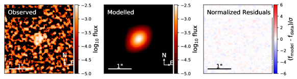
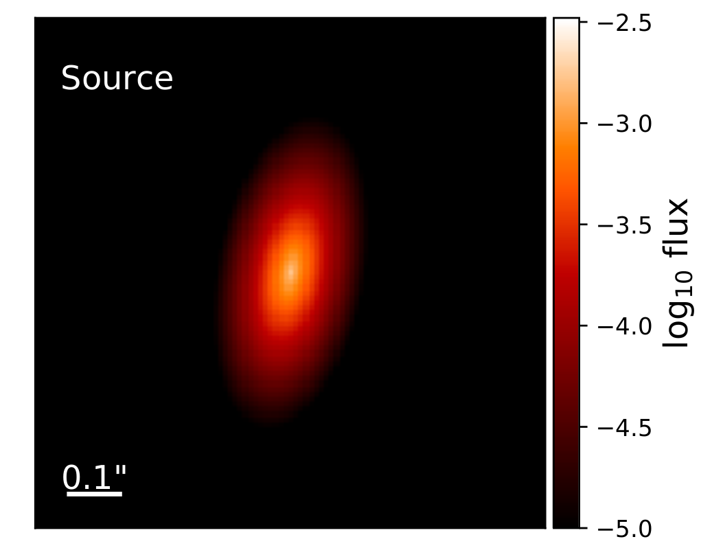
Figure 1: Modeling results of the source Abell1763-1564 using Lenstruction, including the observed (HST/WFC3 F160W) and modelled source in the image plane with normalised residuals and the predicted morphology in the source plane (note that the source plane image is plotted on a different spatial scale), respectively from left to right. The measured size of Abell1763-1564 is $R_{\rm{eff,circ}}=0.515$ kpc.

The targets in this work were also observed with Spitzer Space Telescope via the Spitzer-RELICS program (S-RELICS, PI Bradač #12005, 13165, 13210, PI Soifer, #12123), which collected $>1000$ hours of data in the 3.6$\mu$m and 4.5$\mu$m IRAC bands. 13 clusters were observed to 30-hour depth per Spitzer/IRAC band (3-$\sigma$ depth $\sim$26 mag), using a combination of S-RELICS and archival data. The remaining 27 clusters were observed to 5-hour depth (3-$\sigma$ depth $\sim$24 mag). The details of Spitzer data collection and reduction, as well as a complete catalogue of HST+Spitzer fluxes and a variety of stellar properties for each high-redshift object can be found in Strait et al. (2020). Reduced Spitzer images are available from the NASA/IPAC Infrared Science Archive (IRSA) and all raw data are available for download on the Spitzer Heritage Archive (SHA).

2.2 Lens Models

In order to model the high-redshift galaxies in their source planes, we utilized magnification maps primarily from Glafic (Oguri, 2010) lens models since these maps were avilable for most clusters, and we used Lenstool (Jullo & Kneib, 2009) maps for the remaining clusters. These maps were provided by the RELICS team and are made available for public use on MAST. Because some RELICS clusters lack sufficient constraints to create a lens model, nine of the RELICS clusters (A1300, A520, A665, PLCKG004-19, PLCKG138-10, PLCKG308-20, RXC1514-15, SPT0254-58, WHL0137-8) have no publicly available models, and thus any sources lensed by these clusters are discarded for lack of reliable magnification measurements. For further information regarding these lens models, see Cerny et al., 2018, Acebron et al., 2018, Cibirka et al., 2018, Paterno-Mahler et al., 2018, Acebron et al., 2019b, Matthee et al., 2019, Acebron et al., 2019a, Okabe et al., 2020. It is important to note that size measurements in the presence of lensing can be recovered robustly given an appropriate lens model, as shown by, e.g., Yang et al. (2020b). Further, we will discuss uncertainties due to magnification in detail in Section 3.1.

2.3 Sample Selection

We obtain our sample of galaxies from the RELICS catalogue (Strait et al., 2020), selecting 78 singly imaged high-redshift sources with peak redshift $z\geq 5.5$. We use the photometric redshifts from Method A in Strait et al. (2020). Briefly, these are calculated using a set of seven templates from EA$z$Y (Brammer et al., 2008) in linear combination to estimate the redshift. The average uncertainty on redshift is $\sim 2\%$, calculated from the 68% confidence intervals of the photo-$z$ probability density function (PDF).

From the 207 sources in the Strait et al. (2020) catalogue, we include only sources with reliable Spitzer/IRAC fluxes for accurate spectral energy distribution (SED) fitting, which allows us to more reliably determine stellar masses and star formation rate (SFR). Our sample consists of blue, star-forming galaxies selected using a variety of photometric redshift codes (Salmon et al., 2020; Strait et al., 2020). We limit our study of source sizes to galaxies detected in HST F160W with high signal-to-noise ratio (S/N$>$5) and resolved in the image plane given the HST point-spread-function (PSF) for the Wide Field Camera 3 (WFC3) (MacKenty et al., 2008). We also require the use of reliable lens models to constrain the properties of singly imaged sources as explained above. After these selections, our sample consists of 78 sources from 28 independent lines of sight.

3 Galaxy Size Measurements

To measure the sizes of sources in RELICS clusters, we closely follow the methods of Yang et al. (2020b), utilizing the Python package Lenstruction Yang et al. (2020a), which is based on Lenstronomy (Birrer et al., 2015; Birrer & Amara, 2018). Lenstruction has been proven reliable for source reconstruction and size measurements as tested in Yang et al. (2020b). Throughout this section, we outline the basics of the modeling procedures and uncertainties associated with our assumptions. For more information on the process, we refer the reader to Yang et al. (2020a) as well as the GitHub repositories for Lenstruction and Lenstronomy.

Lenstruction adopts forward modeling, using the appearance of our high redshift galaxies in the image plane to model the morphology in the source plane. Because our sample deals strictly with high-redshift objects, we use F160W images at 30 milliarcsecond resolution for our size measurements, corresponding to $\sim 1.54\rm{\mu m}$ / $(1+z_{\rm{median}})\approx 0.21\rm{\mu m}$ in rest-frame light, where $z_{\rm{median}}=6.2$ is the median redshift of the sample. The measurement thus varies slightly in rest-frame wavelengths in our sample, as we cover a range of redshifts ($5.5\lesssim z\lesssim 10$), but always remains in the rest-frame UV. We select a stellar object in the corresponding cluster’s field to take into account the PSF of the instrumentation, and the modeling process also makes use of lens models (Section 2.2) for consideration of the distortion of each singly-imaged galaxy. We use RMS maps of each cluster made available by RELICS as inputs for the pixel selection of each object and scale these maps by 1.1 to account for correlated noise (see Trenti et al., 2011), although we note that this correction has no significant influences on our results. Lenstruction also removes the background.

We parameterize the light profile of each object’s shape as an elliptical Sérsic profile, with several free parameters including the Sérsic radius, which is the semi-major half light, or effective, radius ($R_{\rm{eff}}$). We fix the Sérsic index at $n_{\rm{Sersic}}$=1 and constrain the ellipticity with an upper limit of $0.9$ in agreement with the methods of Kawamata et al. (2018). The source parameters of the best fit solution produced by Lenstruction provide information about the delensed galaxy from which we measure the effective radius.

Outputs from Lenstruction for an example galaxy in our sample are shown in Figure 1, with observations, the modeled galaxy in the image plane, a residual map, and the predicted morphology of the galaxy in the source plane.

3.1 Biases and Uncertainties

The statistical uncertainties on size measurements are obtained from a Markov chain Monte Carlo (MCMC) process. This process samples over parameters $R_{\rm{eff}}$, eccentricity, and spatial position of the galaxy in the source plane to investigate the confidence intervals of the model and degeneracies among parameters. Results are characterized by a 1$\sigma$ distribution, and errors are included in Figure 3, with an average uncertainty on $R_{\rm{eff}}$ of 53.4%.

One possible bias is induced by our assumption of a Sérsic index of 1. While $n=1$ is perhaps a reasonable assumption for $z\geq 5.5$ galaxies (Petty et al., 2009, Buitrago et al., 2013, Krywult et al., 2017, Bouwens et al., 2022), our data do not have the power to constrain Sérsic indices and therefore this choice may introduce a systematic error in our measurements of effective radii. If we assume a Sérsic index of $n=0.5$ or $n=2$, our half-light radius results differ by an average of less than 6%, and this assumption is thus negligible on the average uncertainty.

To estimate other systematic uncertainties, we apply a series of tests as described below. In our analysis, we assume the peak redshift from the PDF of redshift distribution, calculated from the spectral energy distribution (SED) fitting method described in Strait et al.(2020, Method A), as well as best fit magnification from lens models (described in Section 2.2). There is an uncertainty in both redshift and magnification for each source. We estimate the propagation of these uncertainties on sizes by obtaining the sizes of the sources using the convergence and shear maps from the range of maps calculated by bootstrapping lens modeling constraints, which incorporates those statistical uncertainties. In addition, we randomly select a redshift from the galaxy’s photo-$z$ PDF for each iteration to estimate the effect of the uncertain redshift on our results. We then calculate 68% confidence intervals from the combined magnification and redshift uncertainties and find that these errors contribute less than an additional 10% to size measurement errors. Because these uncertainties are much smaller than those reported from Lenstruction due to uncertainties from lensing itself, the uncertainties from Sérsic index and magnification and redshift are not included in Figure 3.

To calculate the cosmic variance of one RELICS field we use the CosmicVarianceCalculator (Trenti & Stiavelli, 2008), and using inputs of mean redshift and number of objects detected per field, we get a value of 0.3. The total variance reduces by a factor of $\sqrt{N}$, with $N$ being the 28 independent fields our 78 candidates are found within, giving 5.7% as the fractional error on galaxy number counts due to sample variance.

In addition to these uncertainties, we calculate the completeness of our sample to understand our results relative to the what the galaxy population likely is. Though lensing is an incredibly useful tool, understanding incompleteness in lensing fields is more complicated than doing so in blank fields. Specifically, completeness is a function not just of galaxy luminosity and size, but also of magnification and distortion, and thus varies with position with respect to the lensing cluster and the lensing properties of the lensing cluster (e.g., Bouwens et al., 2022).

Using the software GLACiAR2 (Carrasco et al., 2018; Leethochawalit et al., 2022), we calculate source detection completeness as a function of magnitude and size for a typical cluster observation in our sample. We follow the methods in Yang et al. (2022), with the code modified to incorporate effects from gravitational lensing by utilizing available lens models. This software simulates lensed galaxies modeled with a Sérsic profile at random positions in the source plane and predicts their lensed properties in the image plane, calculating the detection recovery fraction in the F160W image. We set bins for absolute magnitude, $M_{\text{UV}}$, from -22 to -16 and sizes, $R_{\text{eff}}$, from $0.03$ to $1$ kpc, as well as redshifts $z\sim 5.5-10$, which are characteristic ranges of our sample. For more details on the process, refer to Yang et al. (2022).

An example of the resulting completeness map for the cluster Abell 1763 at a redshift of $z=7$ is shown in Figure 2. For sources between -19 and -21 $M_{\rm{UV}}$, completeness is about 60-80%. While we are relatively complete for this brighter population of galaxies, our sample is incomplete for the faintest population ($<10$%) and we may be preferentially missing large, faint galaxies.

We make no attempt in this work to constrain the entire population of high redshift galaxies and rather demonstrate that a population of compact galaxies at $z\geq 5.5$ does exist. With JWST, we will improve on incompleteness measurements at high redshift. This goal of this work is to produce an exploration of the distribution of sizes in a sample of star-forming high redshift galaxies rather than to reconstruct the intrinsic size-luminosity and size-mass relations. Therefore we leave a more complete characterization of the population to future work; however, this important caveat should be kept in mind when interpreting our results.

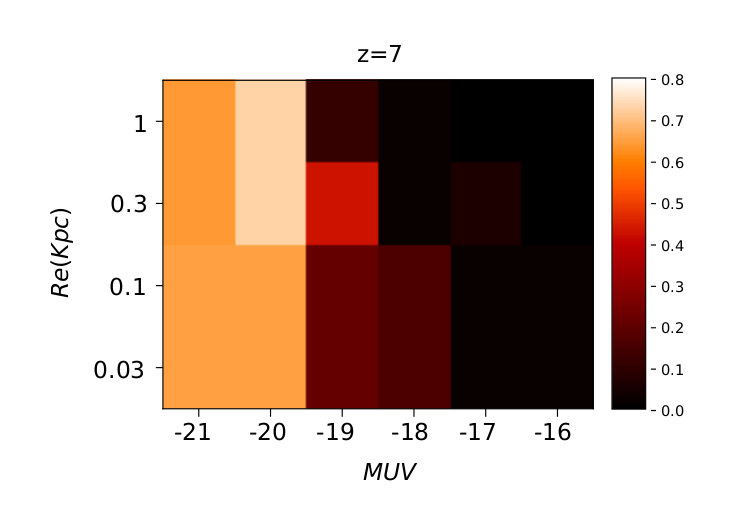
Figure 2: Detection completeness for a typical cluster observation in our sample (Abell 1763). We simulate $z\sim 7$ galaxies with different magnitudes and sizes and measure their recovery fraction (color bar). Our sample is relatively complete ($\geq 50\%$) for brighter galaxies at magnitudes of -19 to -21 and small sizes $<0.3$ kpc, but our sample might be missing large and/or faint galaxies and is very incomplete for the faintest population. Here we show completeness detections for only one redshift ($z=7$) because the redshift dependence within our redshift range is negligible for completeness calculations.

4 Results and Discussion

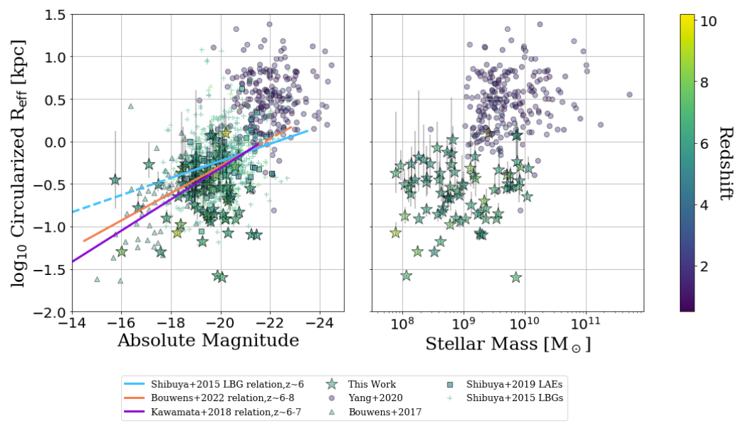
Figure 3: Measured circularised effective radius vs. absolute magnitude (left) and stellar mass (right), with points coloured by redshift. Starred points indicate our data, alongside circles for $z\sim 1-3$ data from Yang et al. (2020b), triangles for Bouwens et al. (2017), and squares (Lyman $\alpha$ emitters) and ’$+$’ points (Lyman break galaxies) for Shibuya et al. (2015); Shibuya et al. (2019). Size-magnitude relations derived by Kawamata et al. (2018), Bouwens et al. (2022), and Shibuya et al. (2015) are shown as purple, orange, and cyan lines respectively on the first plot. Errorbars on size measurements are derived from the MCMC process of Lenstruction described in Section 3.1. We measure small galaxies, similar in size to the other studies and in some cases, brighter.

4.1 Small Sizes

Size measurements and other properties of selected galaxies from our sample are provided in Table 1, and we present our results for the size-magnitude and size-mass measurements of our sample in Figure 3. We analyse our results in the context of previous studies, using the circularised effective radii of our sources ($R_{\rm{eff,circ}}=R_{\rm{maj}}*\sqrt{1-e}$, where $R_{\rm{maj}}$ is our measured effective radius, $e=1-\sqrt{1-c^{2}}$ is ellipticity, and $c$ is eccentricity as determined by the best fit parameters output by Lenstruction). The circularized effective radius is the standard parameter for the size measurements of small, high redshift sources (e.g, Ono et al., 2013; Holwerda et al., 2015; Shibuya et al., 2015; Shibuya et al., 2019). On the left of Figure 3 we plot measured sizes against magnitudes, where starred points are our data, triangles are data from Bouwens et al. (2017) (also used in Bouwens et al., 2022) who uses deeper data, but in fewer lensed fields, and circles are low redshift data from Yang et al. (2020b), and each point is coloured by redshift. Our sample contains brighter galaxies compared to the fainter population from Bouwens et al. (2017), and both measure small sizes ($<200$ pc). We also include sizes of $z\geq 6$ Lyman-$\alpha$ emitters (LAEs) and Lyman break galaxies (LBGs) from Shibuya et al. (2015); Shibuya et al. (2019) as squares and plus signs, respectively. While Shibuya et al. (2019) have a much larger sample of star-forming galaxies, we probe smaller sizes due to lensing.

We also compare our size measurements to previous studies in the context of the size-mass relation of galaxies in Figure 3 on the right. We use median stellar mass measurements as obtained by Strait et al. (2020, Method A), estimated by the median of the probability density function (PDF) of each source. Once again, our data is shown as starred points along with data from Yang et al. (2020b) as circles, coloured by redshift.

The presence of small galaxies is consistent with the results of Bouwens et al. (2017, 2022) and Kawamata et al. (2015), with galaxy sizes on the order of $\sim 30-100$ pc, as well as the small sizes found by Coe et al. (2013) and Zitrin et al. (2014) at the highest redshifts. We include size-luminosity relations derived by Shibuya et al. (2015), Bouwens et al. (2022), and Kawamata et al. (2018) as lines in Figure 3, from which we can see that these small sizes ($R_{\rm{eff}}<200$ pc) result in a steep size-luminosity relation, although a characterization of the incompleteness and selection function are needed to quantify this trend. While our sample is incomplete, these results show that compact star forming galaxies, only slightly larger than typical globular clusters, exist in non-negligible numbers in the early universe.

4.2 Implications for Reionization

We can use our size measurements to compare to other properties of these high-redshift galaxies as well. Through the investigation of these properties, we can gain further insight into the process of reionisation in the early universe and the role of these high-redshift galaxies as possible Lyman continuum leakers.

4.2.1 Star Formation Rate Surface Density and [OIII]+H$\beta$

Previous works have used compact sizes to select for potential Lyman continuum leaking galaxies, including the compact Green Pea galaxies at $z\sim 0.1-0.3$, which are likely relevant local analogs of high-redshift UV galaxies (Cardamone et al., 2009; Kim et al., 2021). Lyman continuum leakers are also thought to be compact and highly star-forming. For example, Marchi et al. (2018) find that UV compact sources ($R_{\text{eff}}<0.3$ kpc) at $z\sim 3.5-4.3$ with high SFR surface density ($\Sigma_{\text{SFR}}$) are likely to have higher Lyman continuum flux than lower surface density galaxies. Additionally, Izotov et al. (2016) find that a sample of $z\sim 0.3$ known Lyman continuum leakers have high SFR surface densities. Other works also find a correlation between Lyman continuum escape fraction and $\Sigma_{\text{SFR}}$ in low-redshift analogs at $z\sim 0.2-0.4$ (Flury et al., 2022) and $z\sim 0.3$ (Verhamme et al., 2017). Using the SFR surface densities of known Lyman continuum galaxies, Naidu et al. (2020) find that Lyman continuum leakers have higher $\Sigma_{\text{SFR}}$ than average galaxies at their respective redshifts. In addition, it has been found that the velocity of ionised outflows is strongly correlated with SFR and $\Sigma_{\text{SFR}}$ (e.g., Heckman et al., 2015; Cicone et al., 2016). While only known to be applicable for lower redshift galaxies that may not be the exact analogs of the high-redshift universe, this is currently one of the best criteria we have to indirectly identify potential Lyman continuum leakers.

We calculate the SFR surface density using the relation $\Sigma_{\rm{SFR}}=\rm{SFR}/(2\pi R_{\text{eff}}^{2})$ (Ono et al., 2013; Shibuya et al., 2019; Naidu et al., 2020; Flury et al., 2022), where SFR is the star formation rate as calculated by Strait et al. (2020, Method A) and $R_{\text{eff}}$ is our measured circularised effective radius of the source. We present the distribution of our sample in the SFR surface density-absolute magnitude plane in Figure 4. As seen in this figure, our sources have high SFR surface densities, as they are at relatively high redshifts and the RELICS survey tends to select relatively bright sources in the UV which generally scales with SFR (Kennicutt, 1998; Lemaux et al., 2021). We also detect some intrinsically faint sources due to lensing. There are several sources with $\Sigma_{\text{SFR}}>10M_{\odot}\text{yr}^{-1}\text{(kpc)}^{-2}$, which is higher than the average for typical galaxies at redshifts $z\sim 6-8$ according to the relation between $\Sigma_{\text{SFR}}$ and redshift found by Naidu et al. (2020) and Shibuya et al. (2015). With high SFR surface densities, these galaxies are potential Lyman continuum leaking candidates.

In addition, a common indicator of galaxies with highly ionised environments is strong H$\beta$ $\lambda$4861Å + [OIII] $\lambda$4959,5007Å emission. This indicator has been used in previous works (e.g., Verhamme et al., 2015; Izotov et al., 2016; Fletcher et al., 2019; Izotov et al., 2021; Malkan & Malkan, 2021) to select Lyman continuum leakers at lower redshifts, and Tang et al. (2019) finds that ionizing photon production increases with higher [OIII] + H$\beta$ EW at $z=1.3-2.4$. Several studies find that high-redshift ($z\gtrsim 7$) galaxies typically have extreme [OIII]+H$\beta$ emission, with equivalent widths greater than 1000Å (e.g., Smit et al., 2015; Roberts-Borsani et al., 2016; Roberts-Borsani et al., 2020). Endsley et al. (2021) also finds that extreme emitters at $z\sim 7$ with a median [OIII] + H$\beta$ EW of $\sim$ 700 Å may be undergoing a short burst of star formation, which increases the escape fraction of ionizing photons.. While Saxena et al. (2021) finds that there is no strong correlation between the [OIII]+H$\beta$ emission of a galaxy alone and its Lyman continuum radiation escape fraction $f_{\rm{esc}}$, [OIII] + H$\beta$ emission is likely a useful tool to select possible Lyman continuum leakers in conjunction with other probes such as $\Sigma_{\rm{SFR}}$. We plot [OIII] + H$\beta$ equivalent widths as a colorbar in Figure 4 for sources with IRAC channel 1 or 2 detections (S/N$>3$) as measured by Strait et al. (2020, Method B). Because [OIII]+H$\beta$ is not well constrained for all objects in our sample, and there is uncertainty on the use of the [OIII]+H$\beta$ EW as a criterion for Lyman continuum leakages, we do not emphasize it as a criterion for our sample.

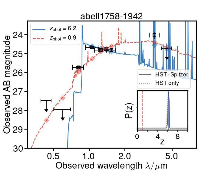
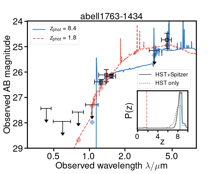
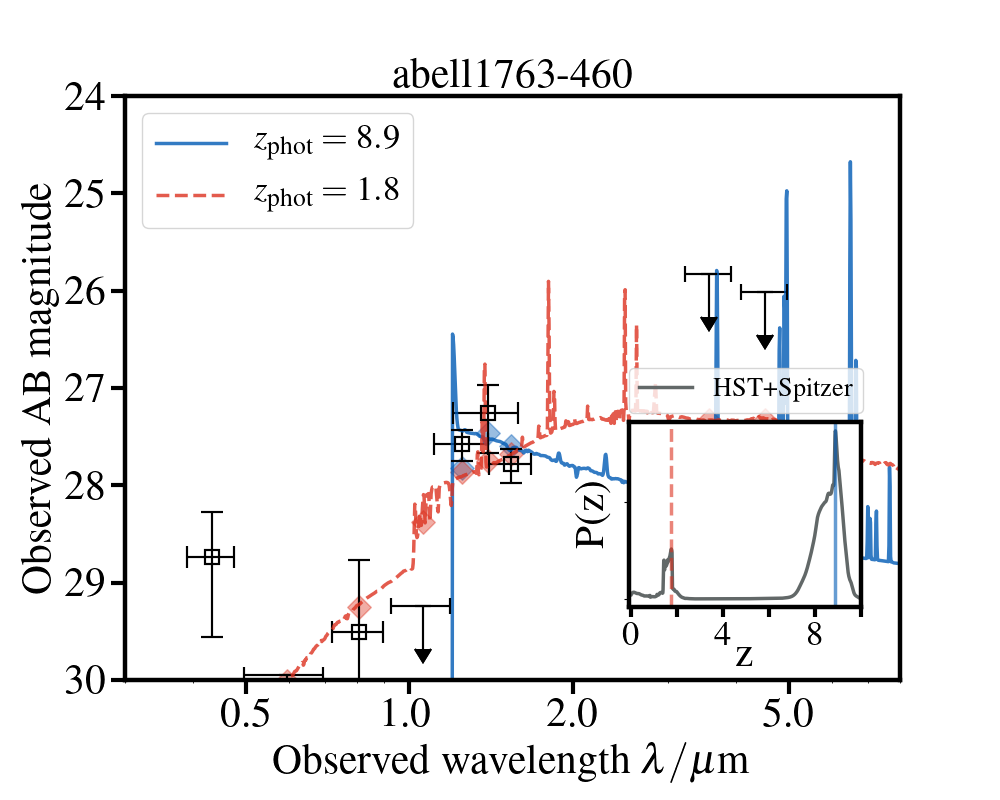
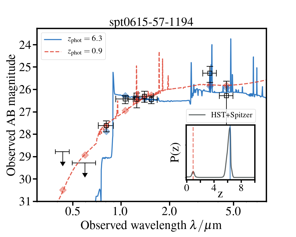
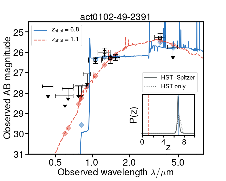
Figure 5: Spectral energy distributions for 14 examples of galaxies with high SFRD and high inferred [OIII]+H$\beta$ emission, obtained using Method A as described by Strait et al. (2020). Black points are data, and blue and red lines are predicted photometry from models using the best-fit high redshift and secondary redshift peak templates, respectively, with the redshift PDF for each source shown in the insets. Each of these galaxies are at similar redshifts ($z\sim 7$), where [OIII]+H$\beta$ fall into the channel 1 filter of Spitzer/IRAC. When extreme in emission, the flux in this filter is boosted. Boosted nebular emission and high SFRD are two qualities that tend to yield Lyman continuum leaking galaxies. It is unknown whether these galaxies are Ly$\alpha$ emitters due to the lack of spectroscopic data of sufficient depth.

We present the best-fit SEDs for a selection of these potential Lyman continuum leaking galaxies, with high SFR surface densities and inferred [OIII]+H$\beta$ EW, in Figure 5. Several of these galaxies show excess emission in channel 1 of Spitzer/IRAC, implying a strong presence of nebular emission. These include the extreme [OIII] emitter, PLCGK287+32-2013 with [OIII] + H$\beta$ EW$\sim 700$Å, highlighted in Strait et al. (2021) and the quadruply imaged galaxy in Zitrin et al. (2017).

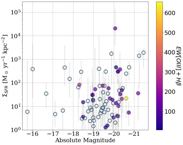
Figure 4: Star formation surface density, calculated using our measurements of circularised effective radius and SFR from Strait et al. (2021), vs. absolute magnitude. There are many sources with SFR surface density $>10$ $M_{\odot}$ yr^-1, which is higher than average for typical galaxies at this redshift increasing the likelihood that these are potential Lyman continuum leakers. Sources are colored based on the colorbar on the right, indicating the values of the [OIII] + H$\beta$ EW for detections (S/N$>$3) in channels 1 or 2 of IRAC.

4.2.2 Lyman $\alpha$ Emission

High [OIII] + H$\beta$ emission likely implies that a galaxy’s interstellar medium (ISM) is more transparent to Lyman continuum photons and points to high specific star formation rate, active galactic nuclei (AGN), or both, which is correlated with the strength of outflows (Chisholm et al., 2017). Ly$\alpha$ emission is another possible probe of the capability of the galaxy to output ionising photons into the surrounding IGM (e.g., Shapley et al., 2016). If Ly$\alpha$ is visible at $z>6$, there must be either a large enough ionised bubble for the Ly$\alpha$ photons to escape or an outflow and leaking Lyman continuum photons. When observed together, strong Ly$\alpha$ and [OIII]+H$\beta$ emission thus indicate a high likelihood for a galaxy to be a Lyman continuum leaker.

The majority of galaxies in this sample do not have sufficiently deep spectral data to have observed Ly$\alpha$ emission with the exception of MS1008-12-427. This is the Dichromatic Primeval Galaxy at $z\sim 7$ (DP7) discovered by Pelliccia et al. (2021). With extreme Ly$\alpha$ emission ($>200$Å  equivalent width) compared to other LAEs at $z\sim 7$ (e.g., Pentericci et al., 2014; Hoag et al., 2019; Fuller et al., 2020), it has the potential to be a Lyman continuum leaker, or to be residing in an ionised bubble nearby a Lyman continuum leaker. Pelliccia et al. (2021) describe the possibility of DP7 being host to two distinct components, one dusty and red, and the other highly star forming and blue, and this possible merger or rejuvination event could lead to a large outflow, producing the strong Ly$\alpha$ emission. The very red SED and distinct UV $\beta$ slopes suggest that a majority of the UV flux comes from the blue component. We measure the combined effective radius of both components, as the sources are blended, but the possibility of two components suggests that the measured size of this source may be that of two distinct objects. Reducing the effective radius by half and attributing all of the UV flux to the bluer component results in double the star formation rate surface density. With $\Sigma_{\text{SFR}}\sim 11^{+55}_{-2}M_{\odot}$ yr^-1 (kpc)^-2, the SFR surface density of DP7 then falls within our selection criterion.

PLCKG287-2013 and the quadruply imaged galaxy 777 have been observed with GMOS Gemini South but no Ly$\alpha$ emission was detected (see Strait et al., 2021, Section 5.4.2 for further details). Regarding the rest of the sample, we can also compare with LAEs from Shibuya et al. (2019) in Figure 3 to infer where LAEs may lie for our sample in the size-magnitude space. If any of these galaxies are Ly$\alpha$ emitters, they could be important sources for understanding the output of ionising photons in the Epoch of Reionisation, as they are compact and highly star-forming. In addition, these sub-L* galaxies are especially important for follow up because, while they are not as bright as galaxies quoted by (Naidu et al., 2021), they can provide further understanding of the contribution of a range of "medium-bright" representative galaxies to reionisation.

Table 1: Size measurements and other selected properties of sources in our sample. Full table including all sources is available in the electronic edition as supplementary material.

Object ID	$z_{\rm{peak}}^{1}$	$M_{\rm{UV}}^{2}$	M${}_{*}^{3}$	$R_{\rm{eff}}^{4}$	$R_{\rm{eff,circ}}^{5}$	$\Sigma_{\rm{SFR}}^{6}$	$\mu^{7}$	[OIII]+H$\beta$ EW 8
		(mag)	($10^{9}$ $M_{\odot}$)	(kpc)	(kpc)	($M_{\odot}$ yr-1 kpc${}^{-2})$
ABELL2813-102	5.67	-19.94	6${}^{+3}_{-6}$	0.33${}^{+0.11}_{-0.08}$	0.29${}^{+0.12}_{-0.06}$	19${}^{+5}_{-18}$	3.5	74${}^{+2}_{-2}$
RXC0949+17-834	5.92	-17.59	0.34${}^{+0.13}_{-0.16}$	0.05${}^{+0.05}_{-0.03}$	0.05${}^{+0.04}_{-0.03}$	444${}^{+3499}_{-366}$	10.3	-
ABELL3192-728	7.00	-18.43	0.08${}^{+0.04}_{-0.05}$	0.5${}^{+0.7}_{-0.3}$	0.4${}^{+0.7}_{-0.2}$	3${}^{+3}_{-2}$	3.1	-
PLCKG209+10-1145	6.00	-19.72	8${}^{+3}_{-3}$	0.6${}^{+0.4}_{-0.3}$	0.60${}^{+0.3}_{-0.3}$	7${}^{+11}_{-5}$	3.0	-
PLCKG209+10-202	6.15	-20.76	1.9${}^{+1.3}_{-1.7}$	0.15${}^{+0.04}_{-0.05}$	0.15${}^{+0.04}_{-0.05}$	453${}^{+345}_{-327}$	3.0	-
PLCKG287+32-2013	7.54	-20.60	9${}^{+5}_{-6}$	0.52${}^{+0.02}_{-0.02}$	0.502${}^{+0.020}_{-0.019}$	22${}^{+3}_{-18}$	4.2	656${}^{+11}_{-11}$
PLCKG287+32-2032	7.90	-16.01	0.18${}^{+0.06}_{-0.12}$	0.06${}^{+0.08}_{-0.04}$	0.05${}^{+0.07}_{-0.04}$	380${}^{+4293}_{-357}$	56.0	-
PLCKG287+32-2235	6.97	-20.61	1.1${}^{+3.4}_{-0.6}$	0.12${}^{+0.023}_{-0.019}$	0.12${}^{+0.021}_{-0.018}$	245${}^{+6}_{-181}$	2.9	-
PLCKG287+32-698	6.86	-20.20	3.5${}^{+0.9}_{-1.4}$	0.124${}^{+0.023}_{-0.019}$	0.123${}^{+0.021}_{-0.018}$	303${}^{+167}_{-214}$	4.8	114${}^{+2}_{-2}$
PLCKG287+32-777	6.93	-20.20	2.3${}^{+0.4}_{-0.9}$	0.124${}^{+0.023}_{-0.019}$	0.123${}^{+0.021}_{-0.018}$	302${}^{+131}_{-203}$	4.2	120${}^{+3}_{-3}$
1 Peak redshift as described in Section 2.3. Photometric errors are described in Strait et al. (2021).
2 Intrinsic absolute magnitude.
3 Stellar mass as described in Section 4.
4 Measured Sérsic (effective) radius in kpc, described in Section 3.
5 Circularized effective radius in kpc, described in Section 4.
6 Star formation surface density as described in Section 4.
7 Magnification, described in Section 2.2.
8 [OIII]+H$\beta$ equivalent width for IRAC S/N>3 detections as measured by Strait et al. (2020, Method B).

5 Conclusions and Future Work

We present size measurements for 78 high-redshift galaxies from RELICS data, imaged by HST and Spitzer, utilizing the code Lenstruction to measure the sizes of these galaxies. Our main results are as follows:

• We analyse the size-magnitude and size-mass measurements in the context of previous studies, finding many compact ($<$ 200 pc) galaxies in agreement with other works. These extremely small sizes seem to imply a steep size-luminosity relation, though definitive conclusions will require detailed studies to properly evaluate completeness.

• We calculate the star formation surface density of these sources using our measured sizes and find several sources with higher than average SFR surface density ($\Sigma_{SFR}>10$ $M_{\odot}$ yr^-1 (kpc)^-2). We highlight galaxies with high SFR surface density and inferred [OIII] + H$\beta$ emission as likely Lyman continuum leakers. These galaxies are good candidates for followup studies with current and future telescopes for further observation to determine the presence of Ly$\alpha$ emission and to provide more insight into the properties of the sources that may have contributed to reionisation.

• We further investigate the properties of these possible Lyman continuum leakers with boosted nebular emission and high SFR densities. These galaxies and others like them present an opportunity for followup with JWST, Gemini, Keck, and the Atacama Large Millimeter/submillimeter Array (ALMA): they are compact, highly star-forming, have larger apparent brightness due to lensing (and are thus easier for followup), and are likely important for reionisation if found to be Lyman continuum leakers. As part of a sub-$L^{*}$, medium-bright sample, further investigations of these galaxies will also complement previous studies on the determination of the objects responsible for reionising the universe.

Further exploration of these and other high-redshift galaxies, especially with space-based Ly$\alpha$ observations with JWST, where skylines are not an issue, and rest-frame optical observations, will yield tighter constraints on measurements of their properties. Measurements of Ly$\alpha$ strength can lend insight into Ly$\alpha$ escape, which is correlated with Lyman continuum escape, and JWST can also provide higher resolution imaging to yield better size measurements. In addition, measurements of nebular emission lines would provide a better understanding of the ionisation radiation fields strengths of [OIII] and [OII], and H$\alpha$ measurements would provide ionising photon production efficiencies. The detailed information from these observations could lend significant insight into the Epoch of Reionisation and the role of objects in reioinsing the early universe.

Data Availability

The data presented in this paper were obtained from the Multimission Archive at the Space Telescope Science Institution (MAST). StScI is operated by the Association of Universities for Research in Astronomy, Inc., under NASA construct NAS5-26555. Support for MAST and non-HST data is provided by the NASA Office of Space Science via grant NAG5-7584 and other grants and contracts.

References

- Acebron et al. (2018) Acebron A., et al., 2018, ApJ, 858, 42
- Acebron et al. (2019a) Acebron A., et al., 2019a, arXiv e-prints, p. arXiv:1912.02702
- Acebron et al. (2019b) Acebron A., et al., 2019b, ApJ, 874, 132
- Atek et al. (2015) Atek H., et al., 2015, ApJ, 814, 69
- Atek et al. (2018) Atek H., Richard J., Kneib J.-P., Schaerer D., 2018, MNRAS, 479, 5184
- Bhatawdekar et al. (2019) Bhatawdekar R., Conselice C. J., Margalef-Bentabol B., Duncan K., 2019, MNRAS, 486, 3805
- Birrer & Amara (2018) Birrer S., Amara A., 2018, Lenstronomy: Multi-purpose gravitational lens modeling software package (ascl:1804.012)
- Birrer et al. (2015) Birrer S., Amara A., Refregier A., 2015, ApJ, 813, 102
- Bouwens et al. (2017) Bouwens R. J., Illingworth G. D., Oesch P. A., Atek H., Lam D., Stefanon M., 2017, ApJ, 843, 41
- Bouwens et al. (2021) Bouwens R. J., Illingworth G. D., van Dokkum P. G., Ribeiro B., Oesch P. A., Stefanon M., 2021, AJ, 162, 255
- Bouwens et al. (2022) Bouwens R. J., Illingworth G. D., van Dokkum P. G., Oesch P. A., Stefanon M., Ribeiro B., 2022, ApJ, 927, 81
- Brammer et al. (2008) Brammer G. B., van Dokkum P. G., Coppi P., 2008, ApJ, 686, 1503
- Buitrago et al. (2013) Buitrago F., Trujillo I., Conselice C. J., Häußler B., 2013, MNRAS, 428, 1460
- Cardamone et al. (2009) Cardamone C., et al., 2009, MNRAS, 399, 1191
- Carrasco et al. (2018) Carrasco D., Trenti M., Mutch S., Oesch P. A., 2018, Publ. Astron. Soc. Australia, 35, e022
- Cerny et al. (2018) Cerny C., et al., 2018, ApJ, 859, 159
- Chisholm et al. (2017) Chisholm J., Orlitová I., Schaerer D., Verhamme A., Worseck G., Izotov Y. I., Thuan T. X., Guseva N. G., 2017, A&A, 605, A67
- Cibirka et al. (2018) Cibirka N., et al., 2018, ApJ, 863, 145
- Cicone et al. (2016) Cicone C., Maiolino R., Marconi A., 2016, A&A, 588, A41
- Coe et al. (2013) Coe D., et al., 2013, ApJ, 762, 32
- Coe et al. (2019) Coe D., et al., 2019, ApJ, 884, 85
- Dayal (2019) Dayal P., 2019, Proceedings of the International Astronomical Union, 15, 43
- Endsley et al. (2021) Endsley R., Stark D. P., Chevallard J., Charlot S., 2021, MNRAS, 500, 5229
- Finkelstein et al. (2019) Finkelstein S. L., et al., 2019, ApJ, 879, 36
- Fletcher et al. (2019) Fletcher T. J., Tang M., Robertson B. E., Nakajima K., Ellis R. S., Stark D. P., Inoue A., 2019, ApJ, 878, 87
- Flury et al. (2022) Flury S. R., et al., 2022, arXiv e-prints, p. arXiv:2201.11716
- Franx et al. (2008) Franx M., van Dokkum P. G., Förster Schreiber N. M., Wuyts S., Labbé I., Toft S., 2008, ApJ, 688, 770
- Fuller et al. (2020) Fuller S., et al., 2020, ApJ, 896, 156
- Grazian et al. (2011) Grazian A., et al., 2011, A&A, 532, A33
- Grazian et al. (2012) Grazian A., et al., 2012, A&A, 547, A51
- Heckman et al. (2015) Heckman T. M., Alexandroff R. M., Borthakur S., Overzier R., Leitherer C., 2015, ApJ, 809, 147
- Hoag et al. (2019) Hoag A., et al., 2019, MNRAS, 488, 706
- Holwerda et al. (2015) Holwerda B. W., Bouwens R., Oesch P., Smit R., Illingworth G., Labbe I., 2015, ApJ, 808, 6
- Huang et al. (2013) Huang K.-H., Ferguson H. C., Ravindranath S., Su J., 2013, ApJ, 765, 68
- Huang et al. (2017) Huang K.-H., et al., 2017, ApJ, 838, 6
- Ishigaki et al. (2018) Ishigaki M., Kawamata R., Ouchi M., Oguri M., Shimasaku K., Ono Y., 2018, ApJ, 854, 73
- Izotov et al. (2016) Izotov Y. I., Schaerer D., Thuan T. X., Worseck G., Guseva N. G., Orlitová I., Verhamme A., 2016, MNRAS, 461, 3683
- Izotov et al. (2021) Izotov Y. I., Worseck G., Schaerer D., Guseva N. G., Chisholm J., Thuan T. X., Fricke K. J., Verhamme A., 2021, MNRAS, 503, 1734
- Jullo & Kneib (2009) Jullo E., Kneib J.-P., 2009, MNRAS, 395, 1319
- Kawamata et al. (2015) Kawamata R., Ishigaki M., Shimasaku K., Oguri M., Ouchi M., 2015, ApJ, 804, 103
- Kawamata et al. (2018) Kawamata R., Ishigaki M., Shimasaku K., Oguri M., Ouchi M., Tanigawa S., 2018, ApJ, 855, 4
- Kennicutt (1998) Kennicutt Robert C. J., 1998, ARA&A, 36, 189
- Kim et al. (2021) Kim K. J., Malhotra S., Rhoads J. E., Yang H., 2021, ApJ, 914, 2
- Krywult et al. (2017) Krywult J., et al., 2017, A&A, 598, A120
- Leethochawalit et al. (2022) Leethochawalit N., Trenti M., Morishita T., Roberts-Borsani G., Treu T., 2022, MNRAS, 509, 5836
- Lemaux et al. (2021) Lemaux B. C., et al., 2021, MNRAS, 504, 3662
- Livermore et al. (2017) Livermore R. C., Finkelstein S. L., Lotz J. M., 2017, ApJ, 835, 113
- Lotz et al. (2017) Lotz J. M., et al., 2017, ApJ, 837, 97
- MacKenty et al. (2008) MacKenty J. W., Kimble R. A., O’Connell R. W., Townsend J. A., 2008, in Oschmann Jacobus M. J., de Graauw M. W. M., MacEwen H. A., eds, Society of Photo-Optical Instrumentation Engineers (SPIE) Conference Series Vol. 7010, Space Telescopes and Instrumentation 2008: Optical, Infrared, and Millimeter. p. 70101F, doi:10.1117/12.790039
- Malkan & Malkan (2021) Malkan M. A., Malkan B. K., 2021, ApJ, 909, 92
- Marchi et al. (2018) Marchi F., et al., 2018, A&A, 614, A11
- Matthee et al. (2019) Matthee J., et al., 2019, ApJ, 881, 124
- Matthee et al. (2021) Matthee J., et al., 2021, arXiv e-prints, p. arXiv:2110.11967
- Morishita et al. (2014) Morishita T., Ichikawa T., Kajisawa M., 2014, ApJ, 785, 18
- Mowla et al. (2019) Mowla L. A., et al., 2019, ApJ, 880, 57
- Naidu et al. (2020) Naidu R. P., Tacchella S., Mason C. A., Bose S., Oesch P. A., Conroy C., 2020, ApJ, 892, 109
- Naidu et al. (2021) Naidu R. P., et al., 2021, arXiv e-prints, p. arXiv:2110.11961
- Oguri (2010) Oguri M., 2010, PASJ, 62, 1017
- Okabe et al. (2020) Okabe T., et al., 2020, MNRAS, 496, 2591
- Oke (1974) Oke J. B., 1974, ApJS, 27, 21
- Ono et al. (2013) Ono Y., et al., 2013, ApJ, 777, 155
- Paterno-Mahler et al. (2018) Paterno-Mahler R., et al., 2018, ApJ, 863, 154
- Pelliccia et al. (2021) Pelliccia D., et al., 2021, ApJ, 908, L30
- Pentericci et al. (2014) Pentericci L., et al., 2014, ApJ, 793, 113
- Petty et al. (2009) Petty S. M., de Mello D. F., Gallagher John S. I., Gardner J. P., Lotz J. M., Mountain C. M., Smith L. J., 2009, AJ, 138, 362
- Postman et al. (2012) Postman M., et al., 2012, ApJS, 199, 25
- Ribeiro et al. (2016) Ribeiro B., et al., 2016, A&A, 593, A22
- Roberts-Borsani et al. (2016) Roberts-Borsani G. W., et al., 2016, ApJ, 823, 143
- Roberts-Borsani et al. (2020) Roberts-Borsani G. W., Ellis R. S., Laporte N., 2020, MNRAS, 497, 3440
- Robertson (2021) Robertson B. E., 2021, arXiv e-prints, p. arXiv:2110.13160
- Salmon et al. (2020) Salmon B., et al., 2020, ApJ, 889, 189
- Saxena et al. (2021) Saxena A., et al., 2021, arXiv e-prints, p. arXiv:2109.03662
- Shapley et al. (2016) Shapley A. E., Steidel C. C., Strom A. L., Bogosavljević M., Reddy N. A., Siana B., Mostardi R. E., Rudie G. C., 2016, ApJ, 826, L24
- Shen et al. (2020) Shen X., Hopkins P. F., Faucher-Giguère C.-A., Alexander D. M., Richards G. T., Ross N. P., Hickox R. C., 2020, MNRAS, 495, 3252
- Shibuya et al. (2015) Shibuya T., Ouchi M., Harikane Y., 2015, ApJS, 219, 15
- Shibuya et al. (2019) Shibuya T., Ouchi M., Harikane Y., Nakajima K., 2019, ApJ, 871, 164
- Smit et al. (2015) Smit R., et al., 2015, ApJ, 801, 122
- Strait et al. (2020) Strait V., et al., 2020, ApJ, 888, 124
- Strait et al. (2021) Strait V., et al., 2021, ApJ, 910, 135
- Tang et al. (2019) Tang M., Stark D. P., Chevallard J., Charlot S., 2019, MNRAS, 489, 2572
- Trenti & Stiavelli (2008) Trenti M., Stiavelli M., 2008, ApJ, 676, 767
- Trenti et al. (2011) Trenti M., et al., 2011, ApJ, 727, L39
- Vanzella et al. (2020) Vanzella E., et al., 2020, MNRAS, 494, L81
- Verhamme et al. (2015) Verhamme A., Orlitová I., Schaerer D., Hayes M., 2015, A&A, 578, A7
- Verhamme et al. (2017) Verhamme A., Orlitová I., Schaerer D., Izotov Y., Worseck G., Thuan T. X., Guseva N., 2017, A&A, 597, A13
- Yang et al. (2020a) Yang L., Birrer S., Treu T., 2020a, MNRAS, 496, 2648
- Yang et al. (2020b) Yang L., Roberts-Borsani G., Treu T., Birrer S., Morishita T., Bradač M., 2020b, MNRAS, 501, 1028
- Yang et al. (2022) Yang L., et al., 2022, arXiv e-prints, p. arXiv:2201.08858
- Yue et al. (2018) Yue B., et al., 2018, ApJ, 868, 115
- Zitrin et al. (2014) Zitrin A., et al., 2014, ApJ, 793, L12
- Zitrin et al. (2017) Zitrin A., et al., 2017, ApJ, 839, L11
- van der Wel et al. (2014) van der Wel A., et al., 2014, ApJ, 788, 28