Gradient flow scale-setting with $N_{f}=2+1+1$ Wilson-clover twisted-mass fermions

Abstract

We present a determination of the gradient flow scales $w_{0}$, $\sqrt{t_{0}}$ and $t_{0}/w_{0}$ in isosymmetric QCD, making use of the gauge ensembles produced by the Extended Twisted Mass Collaboration (ETMC) with $N_{f}=2+1+1$ flavours of Wilson-clover twisted-mass quarks including configurations close to the physical point for all dynamical flavours. The simulations are carried out at three values of the lattice spacing and the scale is set through the PDG value of the pion decay constant, yielding $w_{0}=0.17383(63)$ fm, $\sqrt{t_{0}}=0.14436(61)$ fm and $t_{0}/w_{0}=0.11969(62)$ fm. Finally, fixing the kaon mass to its isosymmetric value, we determine the ratio of the kaon and pion leptonic decay constants to be $f_{K}/f_{\pi}=1.1995(44)$.

1 Introduction

Precise and accurate scale setting is of central importance as lattice QCD calculations target high precision determinations of the hadron spectrum, the nucleon axial radius, precision inputs for electroweak tests of the Standard Model or the hadronic contribution to the muon $g-2$. The lattice scale may enter either relatively to compare calculations at different values of the inverse bare coupling $\beta=6/g_{0}^{2}$, indirectly when used to fix other bare parameters of the theory such as the quark masses or as an absolute scale in the conversion of dimensionful observables to physical units. Depending on the case, its uncertainty either indirecty or directly also propagates to the error estimates of the final results of a given calculation.

The gluonic scales $t_{0}$ [1] and $w_{0}$ [2] have been employed widely as intermediate scales [3, 4, 5, 6, 7, 8, 9, 10, 11, 12] and have also previously been studied specifically in the context of the ETMC [13, 14, 15]. They are attractive because they are comparatively easy to calculate with high statistical precision, do not involve complicated fitting procedures and can easily be integrated into the ensemble production workflow. In this contribution we give some details on our current determinations of these scales and also present our recent calculation of $f_{K}/f_{\pi}$ [16]. We also make use of the scales in the calculation of quark masses from mesonic inputs [17, 18] as well as leptonic meson decay constants [19].

ensemble $\beta$ $V/a^{4}$ $a~{}\mbox{(fm)}$ $a\mu_{\ell}$ $M_{\pi}~{}\mbox{(MeV)}$ $L~{}\mbox{(fm)}$ $M_{\pi}L$ cA211.53.24 $1.726$ $24^{3}\times~{}48$ $~{}0.0947~{}(4)~{}$ $~{}0.00530~{}$ $~{}346.4~{}(1.6)~{}$ $2.27$ $3.99$ cA211.40.24 $24^{3}\times~{}48$ $~{}0.00400~{}$ $~{}301.6~{}(2.1)~{}$ $2.27$ $3.47$ cA211.30.32 $32^{3}\times~{}64$ $~{}0.00300~{}$ $~{}261.1~{}(1.1)~{}$ $3.03$ $4.01$ cA211.12.48 $48^{3}\times~{}96$ $~{}0.00120~{}$ $~{}167.1~{}(0.8)~{}$ $4.55$ $3.85$ cB211.25.24 $1.778$ $24^{3}\times~{}48$ $~{}0.0816~{}(3)~{}$ $~{}0.00250~{}$ $~{}259.2~{}(3.0)~{}$ $1.96$ $2.57$ cB211.25.32 $32^{3}\times~{}64$ $~{}0.00250~{}$ $~{}253.3~{}(1.4)~{}$ $2.61$ $3.35$ cB211.25.48 $48^{3}\times~{}96$ $~{}0.00250~{}$ $~{}253.0~{}(1.0)~{}$ $3.92$ $5.02$ cB211.14.64 $64^{3}\times~{}128$ $~{}0.00140~{}$ $~{}189.8~{}(0.7)~{}$ $5.22$ $5.02$ cB211.072.64 $64^{3}\times~{}128$ $~{}0.00072~{}$ $~{}136.8~{}(0.6)~{}$ $5.22$ $3.62$ cC211.06.80 $1.836$ $80^{3}\times 160$ $~{}0.0694~{}(3)~{}$ $~{}0.00060~{}$ $~{}134.2~{}(0.5)~{}$ $5.55$ $3.78$

Table 1: Overview of the light quark bare mass, $a\mu_{\ell}=a\mu_{u}=a\mu_{d}$, of the pion mass $M_{\pi}$, of the lattice size $L$ and of the product $M_{\pi}L$ for the various ETMC gauge ensembles used in this work. The values of the lattice spacing $a$ and the values of $M_{\pi}$ and $L$ correspond to the absolute scale $w_{0}=0.17383(63)$ fm.

2 Lattice Setup and Statistical Properties

We make use of $N_{f}=2+1+1$ flavours of Wilson-clover twisted-mass fermions tuned to maximal twist, ensuring automatic $\mathcal{O}(a)$-improvement of all physical observables [20, 21]. We employ the tmLQCD software suite [22, 23, 24] linked against an extended version of the QPhiX [25, 26, 27, 28, 29, 30] library as well as DD$\alpha$AMG [31, 32, 33, 34]. Details of our ensembles are given in Table 1 and we refer to Refs.[15, 16, 35] for details on their generation and the corresponding algorithmic setup.

We employ the gradient flow using the Wilson gauge action and use a third-order Runge-Kutta algorithm as proposed in Ref. [1] to evolve the gauge field along the flow time $t/a^{2}$. For the definition of the energy density $\braket{E(t)}$ in our observables, we make use of the clover discretisation of the field tensor, using the notation $\braket{E_{\mathrm{sym}}(t)}$ in what follows. In Figure 1, we show the evolution of $t^{2}\braket{E_{\mathrm{sym}}(t)}$ and the corresponding MD history of the observable at the point $t=t_{0}^{\mathrm{sym}}$ on ensemble cC211.06.80 at the physical point as a representative example across our ensemble landscape.

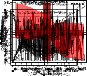
Figure 1: Gradient flow evolution of $t^{2}\braket{E_{\mathrm{sym}}(t)}$ in the determination of $t_{0}^{\mathrm{sym}}$ on the cC211.06.80 ensemble at the physical point (left panel) and the corresponding molecular dynamics history of $t^{2}\braket{E_{\mathrm{sym}}(t)}|_{t=t_{0}^{\mathrm{sym}}}$ (right panel).

We use the Gamma method [36] to estimate our statistical errors. While we do not estimate the exponential tails [37] of the autocorrelation function of our gradient flow observables, we see good error scaling and stable estimates of the integrated autocorrelation time. This is shown exemplarily in Figure 2 for the cB211.14.64 ensemble at a pion mass of around $190$ MeV, where we give the evolution as a function of the number of trajectories $N$ (of length $\tau=1.5$) of the observable $w_{0}/a$, its statistical error and the corresponding estimate of the integrated autocorrelation time. These appear to be reliable from around $\sqrt{N}\sim 30$ onwards.

The results for all observables using the clover discretisation are given in Table 2, where we make use of the shorthand notation $s_{0}=\sqrt{t_{0}}$.

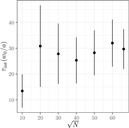
Figure 2: Scaling with the number of trajectories $N$ (of length $\tau=1.5$) of $w_{0}/a$ (left), its statistical error (middle) and the estimate of the integrated autocorrelation time (right, in units of $\tau=1.0$ trajectories) in an analysis on ensemble cB211.14.64. The blue line in the middle panel is a linear fit in the range $30\leq\sqrt{N}\leq 60$.

ensemble $N_{\text{traj}}$ $N_{\text{meas}}$ $s_{0}^{\mathrm{sym}}/a$ $w_{0}^{\mathrm{sym}}/a$ $(t_{0}^{\mathrm{sym}}/w_{0}^{\mathrm{sym}})/a$ $s_{0}^{\mathrm{sym}}/w_{0}^{\mathrm{sym}}$ $\tau_{\textrm{int}}^{s_{0}}$ $\tau_{\textrm{int}}^{w_{0}}$ $\tau_{\textrm{int}}^{t_{0}/w_{0}}$ $\tau_{\textrm{int}}^{s_{0}/w_{0}}$ cA211.53.24 4488 1122 1.5306(21) 1.7597(43) 1.33139(89) 0.86982(100) 23(6) 25(7) 7(1) 18(4) cA211.40.24 4876 1219 1.5384(18) 1.7766(33) 1.33213(96) 0.86592(64) 20(5) 18(4) 7(1) 9(2) cA211.30.32 10236 2559 1.5460( 9) 1.7928(17) 1.33314(47) 0.86233(32) 22(5) 21(4) 9(1) 10(2) cA211.12.48 2608 326 1.5614(22) 1.8249(33) 1.33590(155) 0.85559(29) 69(30) 63(27) 59(25) 16(5) cB211.25.24 4580 1145 1.7937(22) 2.0992(46) 1.53260(108) 0.85445(77) 21(5) 25(6) 5(1) 12(2) cB211.25.32 3960 990 1.7922(19) 2.0991(47) 1.53018(72) 0.85380(91) 35(10) 45(14) 6(1) 28(7) cB211.25.48 4700 1175 1.7915( 8) 2.0982(19) 1.52966(41) 0.85384(38) 28(8) 31(9) 9(2) 20(5) cB211.14.64 4952 619 1.7992( 5) 2.1175(11) 1.52875(23) 0.84968(23) 30(8) 32(9) 8(1) 23(6) cB211.072.64 3065 191 1.8028( 8) 2.1272(19) 1.52784(42) 0.84750(41) 45(18) 52(22) 16(5) 41(16) cC211.06.80 3140 785 2.1094( 8) 2.5045(17) 1.77670(37) 0.84226(27) 46(17) 42(16) 14(3) 26(8)

Table 2: GF scales from the symmetrized action density and corresponding integrated autocorrelation times in units of trajectories of length $\tau=1.0$. The $N_{\text{meas}}$ measurements on each ensemble were performed using different separations in terms of trajectories and the $\tau_{\mathrm{int}}$ were scaled appropriately. Similarly, for the cB211.25.24, cB211.25.32 and cB211.14.64 ensembles, the $\tau_{\mathrm{int}}$ were scaled to take into account the $\tau=1.5$ trajectory lengths used there.

3 Extrapolation to the Physical Point

Before we use the relative scales for further analysis, we follow Ref. [38] and extrapolate to the physical light quark mass at each lattice spacing. Since we have fixed the sea strange and charm quark masses to their physical values to within a few percent, we only parameterise the light quark mass dependence via

$$w_{0}/w_{0}^{\mathrm{phys}}(\beta)=1+c_{\beta}\cdot\left[{\left(M_{\mathrm{PS}}/f_{\mathrm{PS}}\right)}^{2}-{\left(M_{\pi}^{\mathrm{iso}}/f^{\mathrm{iso}}_{\pi}\right)}^{2}\right]\,,$$ (1)

where $w_{0}^{\mathrm{phys}}/a$ and $c_{\beta}$ are fit parameters and where the pion mass $M_{\mathrm{PS}}$ and pion decay constant $f_{\mathrm{PS}}$ have been corrected for finite size effects as detailed in Ref. [16]. The quantities $M_{\pi}^{\mathrm{iso}}$ and $f_{\pi}^{\mathrm{iso}}$ correspond to these quantities in the isosymmetric limit of QCD. The quality of the fit is shown for $w_{0}^{\mathrm{sym}}/a$ in the left panel of Figure 3 and the resulting values of all the relative scales at the physical point are given in the right panel. While we cannot perform this fit for our finest lattice spacing, the single ensemble there is very close to the physical point and we simply use the relative scales as they are.

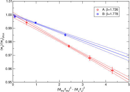
$\beta$ $w_{0}^{\mathrm{sym}}/a$ $\sqrt{t_{0}^{\mathrm{sym}}}/a$ $t_{0}^{\mathrm{sym}}/(w_{0}^{\mathrm{sym}}a)$ $~{}1.726~{}$ $~{}1.8352~{}(35)~{}$ $~{}1.5660~{}(22)$ $~{}1.3359~{}(12)~{}$ $~{}1.778~{}$ $~{}2.1299~{}(16)~{}$ $~{}1.80396~{}(68)$ $~{}1.52789~{}(33)~{}$ $~{}1.836~{}$ $~{}2.5045~{}(17)~{}$ $~{}2.1094~{}(8)$ $~{}1.77670~{}(37)~{}$

Figure 3: Extrapolation to the physical sea light quark mass of $w_{0}/a$ at each lattice spacing using Equation 1 (left) and resulting values of all the relative scales at the physical point (right).

4 Setting the Scale

We first attempt to set the scale via the pion decay constant directly, fitting the data for $w_{0}f_{\pi}(L\to\infty)$ (which has been corrected for finite size effects) using the following functional form

$$w_{0}f_{\pi}(L\to\infty)=w_{0}f\left[1-2\xi\mbox{log}(\xi)+2A_{1}\xi+A_{2}\xi^{2}+\frac{a^{2}}{w_{0}^{2}}\left(D_{0}+D_{1}\xi\right)\right]\,,$$ (2)

where $\xi$ is defined as

$$\xi\equiv\frac{M_{\pi}^{2}(L\to\infty)}{(4\pi f)^{2}}=\frac{(w_{0}M_{\pi})^{2}}{(4\pi w_{0}f)^{2}}~{}\frac{1}{\left[1-\frac{1}{4}\Delta_{\mathrm{FVE}}^{\pi}(L)\right]^{2}}\,,$$ (3)

and where, with respect to a pure NLO ansatz, we have added a possible higher-order term quadratic in $\xi$ as well as discretization effects proportional to $a^{2}$ and $a^{2}M_{\pi}^{2}$. For details we refer to Ref. [16] and show the fit with $A_{2}=0$ in Figure 4 with the result $w_{0}=0.1740(15)$ fm, corresponding to an $0.8$% error.

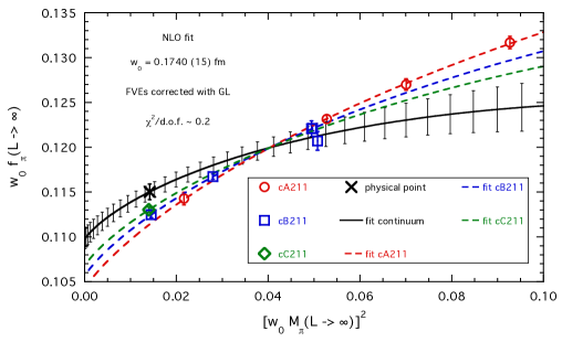
Figure 4: Fit of Equation 2 with $A_{2}=0$ to the data for $w_{0}f_{\pi}$.

In order to better exploit statistical correlations in the data for $f_{\mathrm{PS}}$ and $M_{\mathrm{PS}}$ as well as cancellations of discretisation and finite size effects, we consider the quantity

$$X_{\pi}=\left(f_{\pi}M_{\pi}^{4}\right)^{1/5}\,,$$ (4)

for which we compare the raw data for $w_{0}f_{\mathrm{PS}}$ in the left panel of Figure 5 to the raw data for $w_{0}X_{\mathrm{PS}}$ in the right panel. It is clear that especially the finite size effects are greatly reduced in this combination. We proceed to fit

$$\begin{split}w_{0}X_{\pi}=(w_{0}f)\left\{(4\pi)^{4}\xi^{2}\left[1-2\xi\mbox{log}(\xi)+2A_{1}\xi+A_{2}^{\prime}\xi^{2}+a^{2}\left(D_{0}^{\prime}+D_{1}^{\prime}\xi\right)\right]\right\}^{1/5}\\ \cdot\left(1+F_{\mathrm{FVE}}~{}\xi^{2}e^{-M_{\pi}L}/(M_{\pi}L)^{3/2}\right)\,,\end{split}$$ (5)

the result of which is shown in in the left panel of Figure 6. In the right panel, instead, we have subtracted the resulting continuum curve to better visualise the residual lattice artefacts which are very small and yet very well captured by the fit.

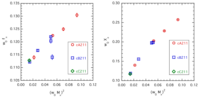
Figure 5: Raw data for the quantities $w_{0}f_{\pi}$ (left) and $w_{0}X_{\pi}$ (right, defined in Equation 4).

For details we again refer to Ref. [16], where different cuts in the data and variations of the higher order terms are used to obtain estimates of systematic errors. Repeating the fits for the scales $w_{0}$, $t_{0}$ and $t_{0}/w_{0}$, we obtain

$$w_{0} =0.17383~{}(57)_{\rm stat+fit}~{}(26)_{\rm syst}~{}[63]~{}\mbox{fm}\,,$$ (6)

$$\sqrt{t_{0}} =0.14436~{}(54)_{\rm stat+fit}~{}(30)_{\rm syst}~{}[61]~{}\mbox{fm}\,,$$ (7)

$$t_{0}/w_{0} =0.11969~{}(52)_{\rm stat+fit}~{}(33)_{\rm syst}~{}[62]~{}\mbox{fm}\,,$$ (8)

with errors added in quadrature and given in square brackets, resulting in an improvement in precision by a factor of about $2.5$ compared to the determination from $f_{\pi}$.

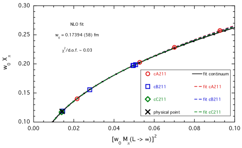
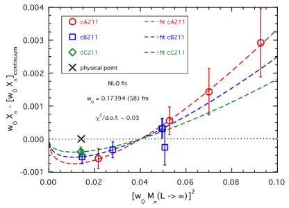
Figure 6: Fit of Equation 5 to the data for $w_{0}X_{\pi}=w_{0}{\left(f_{\pi}M_{\pi}^{4}\right)}^{(1/5)}$ (left) and detail with the resulting continuum curve subtracted to better visualise the very small residual lattice artefacts (right).

The values of the lattice spacing $a$ corresponding to Equations 6, 7 and 8 are given in Table 3. These three determinations of $a$ differ by ${\cal{O}}(a^{2})$ effects, which can be parameterised in their ratios by a function linear in $a^{2}$, as shown in Fig. 7. In particular, we get: $a(\sqrt{t_{0}})/a(w_{0})\simeq 1-0.09\,(2)~{}a^{2}(w_{0})/w_{0}^{2}$ and $a(t_{0}/w_{0})/a(w_{0})\simeq 1-0.18\,(2)~{}a^{2}(w_{0})/w_{0}^{2}$, consistent with $a^{2}$-scaling.

scale	$a_{A}(\beta=1.726)$	$a_{B}(\beta=1.778)$	$a_{C}(\beta=1.836)$
$w_{0}$	0.09471(39)	0.08161(30)	0.06941(26)
$\sqrt{t_{0}}$	0.09217(41)	0.08002(34)	0.06844(29)
$t_{0}/w_{0}$	0.08960(47)	0.07834(41)	0.06737(35)

Table 3: Values of the lattice spacing $a$ (in fm) corresponding to the three GF scales $w_{0}$, $\sqrt{t_{0}}$, $t_{0}/w_{0}$ and to the corresponding relative scales given in the right panel of Figure 3.

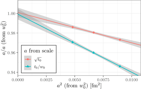
Figure 7: Ratios of lattice spacings determined via $\sqrt{t_{0}}$ and $t_{0}/w_{0}$ with the lattice spacing determined via $w_{0}$ with linear fits superimposed.

5 The ratio $f_{K}/f_{\pi}$

Finally, we employ the lattice spacing determined via $w_{0}/a$ and fixed by $X_{\pi}$ to interpolate our data for $f_{K}/f_{\pi}$ to a reference kaon mass ${(M_{K}^{\mathrm{ref}})}^{2}=(M_{K}^{\mathrm{iso}})^{2}+{(M_{\pi}^{2}-M_{\pi}^{\mathrm{iso}})}^{2}/2$. This interpolated data for $f_{K}/f_{\pi}$ is shown in Figure 8. We further apply finite size corrections as detailed in Ref. [16] and the data using the Ansatz

$$\frac{f_{K}}{f_{\pi}}(L\to\infty)=R_{0}\left[1+\frac{5}{4}\xi\mbox{log}(\xi)+R_{1}\xi+R_{2}\xi^{2}+\frac{a^{2}}{w_{0}^{2}}\left(\widetilde{D}_{0}+\widetilde{D}_{1}\xi\right)\right]\,.$$ (9)

As shown in Figure 9, this results in an excellent fit and we obtain

$$\left(\frac{f_{K}}{f_{\pi}}\right)^{\mathrm{iso}}=1.1995~{}(44)_{\textrm{stat+fit}}~{}(7)_{\textrm{syst}}~{}[44]\,,$$ (10)

at the physical point in the isosymmetric limit of QCD, where again, estimates of the systematic errors are obtained by performing different types of fits and data cuts.

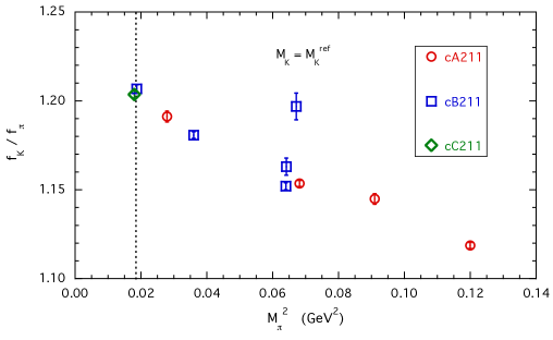
Figure 8: Data for $f_{K}/f_{\pi}$ on all ensembles used in this work interpolated to the reference kaon mass ${(M_{K}^{\mathrm{ref}})}^{2}=(M_{K}^{\mathrm{iso}})^{2}+{(M_{\pi}^{2}-M_{\pi}^{\mathrm{iso}})}^{2}/2$.

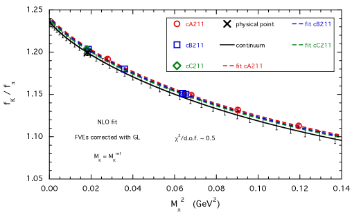
Figure 9: Fit of Equation 9 to the $f_{K}/f_{\pi}$ data shown in Figure 8 corrected for finite size effects.

6 Conclusions and Outlook

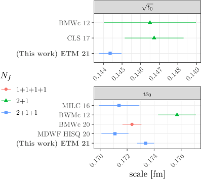
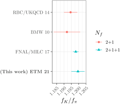
Figure 10: Comparison of the results of this work for the scales $w_{0}$ and $\sqrt{t_{0}}$ from Refs. [2, 9, 10, 12, 8] (left panel) and for $f_{K}/f_{\pi}$ to those from Refs. [39, 40, 41] (right panel).

We conclude by comparing our results for the scales $w_{0}$ and $\sqrt{t_{0}}$ to an incomplete selection from Refs. [2, 9, 10, 12, 8] in the left panel of Figure 10 and our result for $f_{K}/f_{\pi}$ to a selection from Refs. [39, 40, 41] in the right panel. For more complete comparisons we refer to the FLAG review [42]. In future publications we plan to extend the set of ensembles by simulations at a fourth lattice spacing, several more volumes and further values of the light sea quark mass at $\beta=1.836$. An alternative scale setting employing the mass of the omega baryon is currently being studied with the aim of also including QED effects.

References

- [1] M. Lüscher, Properties and uses of the Wilson flow in lattice QCD, JHEP 08 (2010) 071 [1006.4518].
- [2] S. Borsanyi et al., High-precision scale setting in lattice QCD, JHEP 09 (2012) 010 [1203.4469].
- [3] ALPHA collaboration, On the -dependence of gluonic observables, PoS LATTICE2013 (2014) 321 [1311.5585].
- [4] R.J. Dowdall, C.T.H. Davies, G.P. Lepage and C. McNeile, Vus from pi and K decay constants in full lattice QCD with physical u, d, s and c quarks, Phys. Rev. D 88 (2013) 074504 [1303.1670].
- [5] V.G. Bornyakov et al., Wilson flow and scale setting from lattice QCD, 1508.05916.
- [6] HotQCD collaboration, Equation of state in ( 2+1 )-flavor QCD, Phys. Rev. D 90 (2014) 094503 [1407.6387].
- [7] RBC, UKQCD collaboration, Domain wall QCD with physical quark masses, Phys. Rev. D 93 (2016) 074505 [1411.7017].
- [8] MILC collaboration, Gradient flow and scale setting on MILC HISQ ensembles, Phys. Rev. D 93 (2016) 094510 [1503.02769].
- [9] M. Bruno, T. Korzec and S. Schaefer, Setting the scale for the CLS flavor ensembles, Phys. Rev. D 95 (2017) 074504 [1608.08900].
- [10] N. Miller et al., Scale setting the Möbius domain wall fermion on gradient-flowed HISQ action using the omega baryon mass and the gradient-flow scales and , Phys. Rev. D 103 (2021) 054511 [2011.12166].
- [11] ALPHA collaboration, Scale setting for QCD, Eur. Phys. J. C 80 (2020) 349 [2002.02866].
- [12] S. Borsanyi et al., Leading hadronic contribution to the muon magnetic moment from lattice QCD, Nature 593 (2021) 51 [2002.12347].
- [13] A. Deuzeman and U. Wenger, Gradient flow and scale setting for twisted mass fermions, PoS LATTICE2012 (2012) 162.
- [14] ETM collaboration, First physics results at the physical pion mass from Wilson twisted mass fermions at maximal twist, Phys. Rev. D 95 (2017) 094515 [1507.05068].
- [15] C. Alexandrou et al., Simulating twisted mass fermions at physical light, strange and charm quark masses, Phys. Rev. D 98 (2018) 054518 [1807.00495].
- [16] Extended Twisted Mass collaboration, Ratio of kaon and pion leptonic decay constants with Nf=2+1+1 Wilson-clover twisted-mass fermions, Phys. Rev. D 104 (2021) 074520 [2104.06747].
- [17] Extended Twisted Mass collaboration, Quark masses using twisted-mass fermion gauge ensembles, Phys. Rev. D 104 (2021) 074515 [2104.13408].
- [18] C. Alexandrou et al., Determination of the light, strange and charm quark masses using twisted mass fermions, PoS LATTICE2021 (2021) 171 [2110.04588].
- [19] P. Dimopoulos, R. Frezzotti, M. Garofalo and S. Simula, - and -meson leptonic decay constants with physical light, strange and charm quarks by ETMC, PoS LATTICE2021 (2021) 472 [2110.01294].
- [20] ALPHA collaboration, O(a) improved twisted mass lattice QCD, JHEP 07 (2001) 048 [hep-lat/0104014].
- [21] R. Frezzotti and G.C. Rossi, Chirally improving Wilson fermions. 1. O(a) improvement, JHEP 08 (2004) 007 [hep-lat/0306014].
- [22] K. Jansen and C. Urbach, tmLQCD: A Program suite to simulate Wilson Twisted mass Lattice QCD, Comput. Phys. Commun. 180 (2009) 2717 [0905.3331].
- [23] A. Abdel-Rehim, F. Burger, A. Deuzeman, K. Jansen, B. Kostrzewa, L. Scorzato et al., Recent developments in the tmLQCD software suite, PoS LATTICE2013 (2014) 414 [1311.5495].
- [24] A. Deuzeman, K. Jansen, B. Kostrzewa and C. Urbach, Experiences with OpenMP in tmLQCD, PoS LATTICE2013 (2014) 416 [1311.4521].
- [25] B. Joó, D. Kalamakar, K. Vaidyanathan, M. Smelyanskiy, T. Kurth, A. Walden et al.https://github.com/JeffersonLab/qphix .
- [26] B. Joó, D.D. Kalamkar, K. Vaidyanathan, M. Smelyanskiy, K. Pamnany, V.W. Lee et al., Lattice qcd on intel® xeon phitm coprocessors, in Supercomputing, J.M. Kunkel, T. Ludwig and H.W. Meuer, eds., (Berlin, Heidelberg), pp. 40–54, Springer Berlin Heidelberg, 2013.
- [27] M. Schröck, S. Simula and A. Strelchenko, Accelerating Twisted Mass LQCD with QPhiX, PoS LATTICE2015 (2016) 030 [1510.08879].
- [28] B. Joó, D.D. Kalamkar, T. Kurth, K. Vaidyanathan and A. Walden, Optimizing wilson-dirac operator and linear solvers for intel® knl, in International Conference on High Performance Computing, pp. 415–427, Springer, 2016.
- [29] B. Joo, M. Smelyanskiy, D.D. Kalamkar and K. Vaidyanathan, Wilson dslash kernel from lattice qcd optimization, Tech. Rep. Thomas Jefferson National Accelerator Facility (TJNAF), Newport News, VA … (2015).
- [30] S. Heybrock, B. Joó, D.D. Kalamkar, M. Smelyanskiy, K. Vaidyanathan, T. Wettig et al., Lattice qcd with domain decomposition on intel® xeon phi co-processors, in SC ’14: Proceedings of the International Conference for High Performance Computing, Networking, Storage and Analysis, pp. 69–80, 2014, DOI.
- [31] A. Frommer, K. Kahl, S. Krieg, B. Leder and M. Rottmann, Adaptive Aggregation Based Domain Decomposition Multigrid for the Lattice Wilson Dirac Operator, SIAM J. Sci. Comput. 36 (2014) A1581 [1303.1377].
- [32] A. Frommer, K. Kahl, S. Krieg, B. Leder and M. Rottmann, An adaptive aggregation based domain decomposition multilevel method for the lattice wilson dirac operator: multilevel results, 1307.6101.
- [33] C. Alexandrou, S. Bacchio, J. Finkenrath, A. Frommer, K. Kahl and M. Rottmann, Adaptive Aggregation-based Domain Decomposition Multigrid for Twisted Mass Fermions, Phys. Rev. D 94 (2016) 114509 [1610.02370].
- [34] C. Alexandrou, S. Bacchio and J. Finkenrath, Multigrid approach in shifted linear systems for the non-degenerated twisted mass operator, Comput. Phys. Commun. 236 (2019) 51 [1805.09584].
- [35] J. Finkenrath, C. Alexandrou, S. Bacchio, P. Dimopoulos, R. Frezzotti, K. Jansen et al., Twisted mass gauge ensembles at physical values of the light, strange and charm quark masses, PoS LATTICE2021 (2021) 284.
- [36] ALPHA collaboration, Monte Carlo errors with less errors, Comput. Phys. Commun. 156 (2004) 143 [hep-lat/0306017].
- [37] ALPHA collaboration, Critical slowing down and error analysis in lattice QCD simulations, Nucl. Phys. B 845 (2011) 93 [1009.5228].
- [38] O. Bar and M. Golterman, Chiral perturbation theory for gradient flow observables, Phys. Rev. D 89 (2014) 034505 [1312.4999].
- [39] S. Dürr, Z. Fodor, C. Hoelbling, S.D. Katz, S. Krieg, T. Kurth et al., Ratio in qcd, Phys. Rev. D 81 (2010) 054507.
- [40] RBC and UKQCD Collaborations collaboration, Domain wall qcd with physical quark masses, Phys. Rev. D 93 (2016) 074505.
- [41] A. Bazavov et al., - and -meson leptonic decay constants from four-flavor lattice QCD, Phys. Rev. D 98 (2018) 074512 [1712.09262].
- [42] Y. Aoki et al., FLAG Review 2021, 2111.09849.
- [43] Jülich Supercomputing CentreJournal of large-scale research facilities A132 (2018) .
- [44] Jülich Supercomputing CentreJournal of large-scale research facilities A135 (2019) .