Ergodic aspects of trading with threshold strategies

Abstract

To profit from price oscillations, investors frequently use threshold-type strategies where changes in the portfolio position are triggered by some indicators reaching prescribed levels.

In this paper we investigate threshold-type strategies in the context of ergodic control. We make the first steps towards their optimization by proving ergodic properties of related functionals. Assuming Markovian price increments satisfying a minorization condition and (one-sided) boundedness we show, in particular, that for given thresholds, the distribution of the gains converges in the long run.

We also extend recent results on the stability of overshoots of random walks from the i.i.d. increment case to Markovian increments, under suitable conditions.

Keywords: Minorization, random walk, stochastic stability, threshold-type strategies, optimal investment.

1 Introduction

Perhaps the most naive approach to speculative trading is trying to “buy low and sell high” a given financial asset. More refined versions of such strategies are actually widely used by practitioners, see [3, 1, 2]. Their various aspects have been analysed in several papers, see e.g. [8, 20, 21, 22] and our literature review in Section 3.

We intend to study such strategies in a different setting: that of ergodic control. A rigorous mathematical formulation turns out to pose thorny questions about the ergodicity of certain processes, as we shall point out below.

The present article starts to build a reasonable and mathematically sound framework for investigating such problems. We establish that key functionals converge to an invariant distribution and obey a law of large numbers. We are unaware of any previous study that would tackle these questions. Our results may serve as a basis for further related investigations, using techniques of ergodic and adaptive control.

We also investigate a closely related object, studied in [13, 14]: the so-called overshoot process. We extend certain results from [13] from i.i.d. to Markovian summands.

The paper is organized as follows: In Section 2, we state our main results on the stability of level crossings and related quantities of random walks with Markovian martingale differences satisfying minorization and (one-sided) boundedness. In Section 3, we explain the financial setting and the significance of our results in studying optimal trading with threshold strategies. Section 4 presents our results about overshoots. Section 5 contains the proofs of the main results. Section 6 dwells upon future directions of research.

2 Stability of level crossings

Let $M>0$ and let $(X_{n})_{n\in\mathbb{N}}$ be a time-homogeneous Markov chain on the probability space $(\Omega,\mathcal{F},\mathbb{P})$ with state space $\mathcal{X}:=(-\infty,M]$. Its transition kernel is denoted $P:\mathcal{X}\times\mathcal{B}(\mathcal{X})\to[0,1]$. We consider the random walk

$$S_{n}=S_{0}+X_{1}+\ldots+X_{n},$$ (1)

where $S_{0}$ is a random variable independent of $\sigma(X_{k}:\,k\in\mathbb{N})$.

The next minorization condition ensures that the chain jumps, with positive probability, in one step to a small neighborhood of zero independently of the initial state. Moreover, the random movements of $S$ have a diffuse component.

Assumption 2.1.

There exist $\alpha,h>0$ such that, for all $x\in\mathcal{X}$ and $A\in\mathcal{B}(\mathcal{X})$,

$$P(x,A)\geq\alpha\ell(A)$$ (2)

holds where

$$\ell(A):=\frac{1}{2h}\mathrm{Leb}\left([-h,h]\cap A\right)$$

is the normalized Lebesgue measure on $[-h,h]$.

Lemma 2.2.

Under Assumption 2.1, there is a unique probability $\pi_{*}$ on $\mathcal{B}(\mathcal{X})$ such that $\mathrm{Law}(X_{n})\to\pi_{*}$ in total variation as $n\to\infty$, at a geometric speed.

Proof.

Assumption (2) implies that the state space $\mathcal{X}$ is a small set. Hence the chain is uniformly ergodic by Theorem 16.2.2 of [12]. ∎

Assumption 2.3.

For each $z\in\mathcal{X}$,

$$\int_{\mathcal{X}}|x|\,P(z,\mathrm{d}x)<\infty$$

and

$$\int_{\mathcal{X}}x\,P(z,\mathrm{d}x)=0,$$

Remark 2.4.

Clearly, Assumption 2.3 guarantees that $X_{n}$, $n\in\mathbb{N}$, if integrable, is a martingale difference sequence and the limit distribution of Lemma 2.2 has zero mean, that is,

$$\int_{\mathcal{X}}x\,\pi_{*}(\mathrm{d}x)=0.$$

Let us fix thresholds $\underline{\theta},\overline{\theta}\in\mathbb{R}$, satisfying $\underline{\theta}<0<\overline{\theta}$. Furthermore, we define the sequence of crossing times corresponding to $\underline{\theta}$ and $\overline{\theta}$ by the recursion $L_{0}:=0$ and for $n\in\mathbb{N}$,

$$T_{n+1}:=\min\{k>L_{n}:\ S_{k}<\underline{\theta}\},\quad L_{n+1}:=\min\{k>T_{n+1}:\ S_{k}>\overline{\theta}\}.$$ (3)

Lemma 2.5.

Let $EX_{n}^{2}<\infty$ hold for all $n\geq 1$. (This is the case, in particular, if the $X_{n}$ are bounded.) Under Assumptions 2.1 and 2.3, the random variables $T_{n},L_{n}$ are well-defined and almost surely finite.

Proof.

We will prove the statement inductively, the first step being trivial since $L_{0}<\infty$. Assume that the statement has been shown for $L_{0},L_{1},T_{1},\ldots,L_{n}$ and we go on showing it for $T_{n+1}$ and $L_{n+1}$.

In the induction step, we work on the events $B_{k}:=\{L_{n}=k\}$, $k\in\mathbb{N}$ separately. Fixing $k$, the process $M_{j}:=\sum_{l=0}^{j}\mathds{1}_{B_{k}}X_{k+l}$, $j\in\mathbb{N}$ is a square-integrable martingale (remember Remark 2.4) with conditional quadratic variation

$$Q_{j}:=\mathbb{E}[(M_{j}-M_{j-1})^{2}\mid\sigma(M_{i},i\leq j-1)]\geq\mathds{1}_{B_{k}}\frac{\alpha}{2h}\int_{-h}^{h}y^{2}\,dy=\mathds{1}_{B_{k}}\frac{\alpha h^{2}}{3},$$

using Assumption 2.1. Hence $\sum_{j=1}^{\infty}Q_{j}=\infty$ almost surely on $B_{k}$. Proposition VII-3-9. of [15] implies that $\liminf_{j\to\infty}M_{j}=-\infty$ on $B_{k}$. It follows that, on $B_{k}$, almost surely

$$\liminf_{j\to\infty}\,(S_{0}+X_{1}+\ldots+X_{L_{n}}+\ldots+X_{L_{n}+j})=-\infty$$

which implies, in particular, $T_{n+1}<\infty$ on $B_{k}$. A similar argument establishes that also $P(L_{n+1}<\infty)=1$. ∎

Although $X_{T_{1}}$ can be positive when $S_{0}<\underline{\theta}$, for $n\geq 2$, $X_{T_{n}}$ is always negative. Moreover it is also straightforward to verify that the process

$$U_{n}:=(X_{T_{n}},S_{T_{n}},X_{L_{n}},S_{L_{n}},L_{n}-T_{n}),\ n\geq 2,$$

is a time-homogeneous Markov chain on the state space

$$\mathcal{U}:=(-\infty,0)\times(-\infty,\underline{\theta})\times(0,M]\times(\overline{\theta},\overline{\theta}+M)\times(\mathbb{N}\setminus\{0\}).$$

The next theorem states that under our standing assumptions, the law of $U_{n}$ converges to a unique limiting law, as $n\to\infty$, moreover, bounded functionals of $U_{n}$ admit an ergodic behavior.

Theorem 2.6.

Let $EX_{n}^{2}<\infty$ hold for all $n\geq 1$. Under Assumptions 2.1 and 2.3, there exists a probability $\upsilon$ on $\mathcal{B}(\mathcal{U})$ such that $\mathrm{Law}(U_{n})\to\upsilon$ at a geometric speed in total variation as $n\to\infty$. Furthermore, for any bounded and measurable function $\phi:\mathcal{U}\to\mathbb{R}$,

$$\frac{\sum_{j=1}^{n}\phi(U_{j})}{n}\to\int_{\mathcal{U}}\phi(u)\,\upsilon(\mathrm{d}u),\ n\to\infty,$$ (4)

almost surely.

Proof.

See in Section 5. ∎

A “mirror image” of the proof of Theorem 2.6 establishes the following result, the “symmetric pair” of Theorem 2.6.

Theorem 2.7.

Let $\tilde{X}_{t}$, $t\in\mathbb{N}$ be a Markov chain on the state space $[-M,\infty)$ for some $M>0$ and define $\tilde{S}_{n}:=S_{0}+\sum_{k=1}^{n}\tilde{X}_{k}$. Let $E\tilde{X}_{n}^{2}<\infty$ hold for all $n\geq 1$. Let Assumptions 2.1 and 2.3 hold for $\tilde{X}_{t}$ Then the recursively defined quantities $\tilde{T}_{0}:=0$ and

$$\tilde{L}_{n+1}:=\min\{k>\tilde{T}_{n}:\ \tilde{S}_{k}>\overline{\theta}\},\quad\tilde{T}_{n+1}:=\min\{k>\tilde{L}_{n+1}:\ \tilde{S}_{k}<\underline{\theta}\}$$ (5)

are well-defined and finite. Furthermore, there exists a probability $\upsilon$ on $\mathcal{B}(\tilde{\mathcal{U}})$ such that $\mathrm{Law}(\tilde{U}_{n})\to\upsilon$ at a geometric speed in total variation as $n\to\infty$, where

$$\tilde{U}_{n}:=(\tilde{X}_{\tilde{L}_{n}},\tilde{S}_{\tilde{L}_{n}},\tilde{X}_{\tilde{T}_{n}},\tilde{S}_{\tilde{T}_{n}},\tilde{T}_{n}-\tilde{L}_{n}),\ n\geq 2$$

is a homogeneous Markov chain on the state space

$$\tilde{\mathcal{U}}:=(0,\infty)\times(\overline{\theta},\infty)\times[-M,0)\times(\underline{\theta}-M,\underline{\theta})\times(\mathbb{N}\setminus\{0\}).$$

For any bounded and measurable function $\phi:\tilde{\mathcal{U}}\to\mathbb{R}$,

$$\frac{\sum_{j=1}^{n}\phi(\tilde{U}_{j})}{n}\to\int_{\tilde{\mathcal{U}}}\phi(u)\,\upsilon(\mathrm{d}u),\ n\to\infty,$$ (6)

almost surely. $\Box$

3 Trading with threshold strategies

Let the observed price of an asset be denoted by $A_{t}$ at time $t\in\mathbb{N}$. We may think of the price of a futures contract, for instance. Positive prices can also be handled, see Remark 3.4 below. We assume a simple dynamics:

$$A_{t}=\mu t+S_{t},$$ (7)

where $\mu\in\mathbb{R}$, $S_{0}\in\mathbb{R}$ are constants and $S_{t}:=S_{0}+\sum_{j=1}^{t}X_{j}$ for a Markov process $X$ with values in $[-M,M]$ for some $M>0$ and satisfying Assumptions 2.1 and 2.3.

In this price model, $\mu t$ represents the drift (or “trend”) and $S_{t}$ performs fluctuations around the trend (the martingale part). The minorization condition (2) is easy to interpret: whatever the current increment $x\in[-M,M]$ of the fluctuations $S$ is, with a positive probability the next increment will be small (that is, the price change will be close to $0$) and the movements of $S$ are diffuse, more precisely, they have a diffuse component.

The practical situation we have in mind is an algorithm that tries to “buy low and sell high” an asset at high (but not ultra-high) frequencies, revising the portfolio, say, once every second or every minute. Such an algorithm is run continuously during the trading day which can be considered a “stationary” environment as economic fundamentals do not change significantly on such timescales.

It seems that ergodic stochastic control is the right settings for such investment problems: the algorithms does the same thing “forever” and its average perfomance should be optimized. We remark that $\mu$ in such a setting is negligible and can safely be assumed $0$, as often done in papers on high-frequency trading. Our results work nevertheless for arbitrary $\mu$ which is of interest for trading on different timescales (e.g. daily revision of a portfolio for several months).

Now we set up the elements of our trading mechanism. Let the thresholds $\underline{\theta},\overline{\theta}\in\mathbb{R}$ be fixed, satisfying $\underline{\theta}<0<\overline{\theta}$. We interpret $\underline{\theta}$ as a level for $S_{t}$ under which it is advisable to buy the asset. Analogously, it is recommended to sell the asset if $S_{t}$ exceeds $\overline{\theta}$. Thus, to realize a “buying low, selling high”-type strategy, the asset should be bought at the times $T_{n}$, $n\geq 1$ and sold at the times $L_{n}$, $n\geq 1$, realizing the profit

$$A_{L_{n}}-A_{T_{n}}=S_{L_{n}}-S_{T_{n}}+\mu(L_{n}-T_{n}).$$ (8)

We now explain the significance of Theorem 2.6 in studying optimal trading with threshold strategies. An investor aims to maximize in $\underline{\theta},\overline{\theta}$ the long-term average utility from wealth, that is,

$$\limsup_{n\to\infty}\frac{\sum_{k=1}^{n}\left[u(S_{L_{k}(\theta)}-S_{T_{k}(\theta)}+\mu(L_{k}(\theta)-T_{k}(\theta)))-p(L_{k}(\theta)-T_{k}(\theta))\right]}{n},$$ (9)

where $u:\mathbb{R}\to\mathbb{R}$ is a utility function and $L_{k}(\theta),T_{k}(\theta)$ refer to the respective stopping times defined in terms of the parameter $\theta=(\underline{\theta},\overline{\theta})$. The function $p:\mathbb{R}_{+}\to\mathbb{R}_{+}$ serves to penalize long waiting times.

Remark 3.1.

If the price is modelled by processes with continuous trajectories, as in [6, 8, 20, 22] then the thresholds are hit precisely and the profit realized between $T_{n}$ and $L_{n}$ is exactly $\overline{\theta}-\underline{\theta}$. In the present setting (just like in the case of continuous-time processes with jumps), the profit realized may be significantly different due to the overshoot (resp. undershoot) of the level $\overline{\theta}$ (resp. $\underline{\theta}$). From the point of view of ergodic control, it is crucial to establish that these overshoots/undershoots tend to a limiting law, which is the central concern of our present paper.

According to Theorem 2.6, the limsup in the above expression is, in fact, a limit, for a large class of $u$, $p$. One could easily incorporate various types of transaction costs in the model.

Example 3.2.

Let $u,p$ be non-decreasing functions that are bounded from above (e.g. $u$ can be the exponential utility, expressing high risk-aversion), and assume $\mu\geq 0$. Since $S_{L_{k}}-S_{T_{k}}$ is necessarily bounded from below, (6) holds with the choice $\phi(U_{n}):=u(S_{L_{k}}-S_{T_{k}}+\mu(L_{k}-T_{k}))-p(L_{k}-T_{k})$ and the limsup is a limit in (11) above.

Remark 3.3.

In the alternative setting of Theorem 2.7 above (with $\tilde{X}_{n}=X_{n}$), the trader sells one unit of the financial asset at $\tilde{L}_{n}$ (shortselling) and then closes the position at $\tilde{T}_{n}$ thus realizing a profit

$$-(A_{\tilde{T}_{n}}-A_{\tilde{L}_{n}})=S_{\tilde{L}_{n}}-S_{\tilde{T}_{n}}-\mu(\tilde{L}_{n}-\tilde{T}_{n}).$$ (10)

This is the analogue (with short positions) of the long-position strategy realizing (8). Theorem 2.7 implies that

$$\limsup_{n\to\infty}\frac{\sum_{k=1}^{n}\left[u(S_{\tilde{L}_{k}(\theta)}-S_{\tilde{T}_{k}(\theta)}+\mu(\tilde{L}_{k}(\theta)-\tilde{T}_{k}(\theta)))-{}p(\tilde{L}_{k}(\theta)-\tilde{T}_{k}(\theta))\right]}{n}$$ (11)

is a limit in this case, too.

In future work, we intend to optimize $\underline{\theta},\overline{\theta}$ by means of adaptive control, using recursive schemes such as the Kiefer-Wolfowitz algorithm, see [23] and Section 6 of [17]. To prove the convergence of such procedures, it is a prerequisite that the process ${S_{L_{k}}-S_{T_{k}}+\mu(L_{k}-T_{k})}$, $k\in\mathbb{N}$ has favorable ergodic properties. This is precisely the content of Theorem 2.6 above.

Remark 3.4.

In an alternative setting, $A_{t}$ may model the logprice of an asset. In that case investing one dollar between $T_{n}$ and $L_{n}$ yields $\exp\left(S_{L_{n}}-S_{T_{n}}+\mu(L_{n}-T_{n})\right)$ dollars. Let $u:(0,\infty)\to\mathbb{R}$, $p:\mathbb{R}_{+}\to\mathbb{R}_{+}$ be non-decreasing functions, $p$ bounded and $u$ bounded from above (such as a negative power utility function). In this setting the optimization

$$\max_{\underline{\theta},\overline{\theta}}\limsup_{n\to\infty}\frac{\sum_{k=1}^{n}\left[u(\exp\left(S_{L_{k}(\theta)}-S_{T_{k}(\theta)}+\mu(L_{k}(\theta)-T_{k}(\theta))\right))-p(L_{k}(\theta)-T_{k}(\theta))\right]}{n}$$

corresponds to maximizing the utility of the long-term investment of one dollar (minus an impatience penalty), using threshold strategies controlled by $\theta$. When $\mu\geq 0$, the limsup is a limit, again by Theorem 2.6.

We briefly compare our approach to existing ones. We do not survey the large literature on switching problems, see Chapter 5 of [16], only some of the directly related papers. Formulations as optimal stopping problems with discounting appear e.g. in [18, 8, 22]. Sequential buying and selling decisions are considered for mean-reverting assets in [21] and [19]. Mean-reversion trading is also analysed in [11]. [20] treats a general diffusion setting, again using discounting.

In our setting of intraday trading discounting is not an appealing option: on such timescales the decrease of the value of future money is not manifested. Here the ergodic control of averages seems more natural an objective to us. Recall also [6] exploring high-frequency perspectives maximizing expectation on a finite horizon (without discounting).

All the above mentioned papers are about diffusion models where the phenomenon of “overshooting” and “undershooting” does not appear. They are, on the contrary, the main focus of the present work. Similar problems seem to come up in an ergodic control setting for continuous-time price processes with jumps. We are unaware of any related studies.

4 Stability of overshoots

In [13] the authors consider a zero-mean i.i.d. sequence $X_{n}$, $n\geq 1$ and a random variable $S_{0}$ independent of the $X_{t}$. They determine the (stationary) limiting law $\mu_{*}$ for the Markov process of overshoots defined by $O_{0}:=\max(S_{0},0)$,

$$O_{n}=S_{L_{n}},\ n\geq 1$$

where $L_{n},T_{n}$ are defined as in (3) but with the choice $\underline{\theta}=\overline{\theta}=0$. They also establish the convergence of $\mathrm{Law}(O_{n})$ to $\mu_{*}$ under suitable conditions. Generalizations to entrance Markov chains on more general state spaces have been obtained in [14].

Using methods of the present paper, we may obtain generalizations into another direction: we may relax the independence assumption on the $X_{t}$.

Theorem 4.1.

Under Assumption 2.1 and 2.3, there exists a probability $\upsilon$ on $\mathcal{B}((0,\infty))$ such that $\mathrm{Law}(O_{n})\to\upsilon$ at a geometric speed in total variation as $n\to\infty$. Furthermore, for any bounded and measurable function $\phi:(0,\infty)\to\mathbb{R}$,

$$\frac{\sum_{j=1}^{n}\phi(O_{j})}{n}\to\int_{(0,\infty)}\phi(u)\,\upsilon(\mathrm{d}u),\ n\to\infty,$$ (12)

almost surely.

Proof.

See in Section 5. ∎

Remark 4.2.

In the i.i.d. case Theorem 4.1 applies if $X_{t}$ is square-integrable, bounded from above and the law of $X_{t}$ dominates constant times the Lebesgue measure in a neighbourhood of $0$. In [13] a much larger class of i.i.d. random variables is treated. On the other hand, we can handle Markovian summands unlike [13].

5 Proofs

Proof of Theorem 2.6.

Iterated random function representation of Markov chains on standard Borel spaces is a commonly used construction, see e.g. [5, 4]. A similar representation for $(X_{n})_{n\in\mathbb{N}}$ is shown in Lemma 5.1 below which will play a crucial role in the proof. Although the proof is quite standard, we present it for the reader’s convenience.

Lemma 5.1.

Let $(\xi_{n})_{n\in\mathbb{N}}$ and $(\eta_{n})_{n\in\mathbb{N}}$ be i.i.d. sequences, independent of each other, and also independent of $\sigma(X_{0},S_{0})$, moreover let $\xi_{0},\eta_{0}$ be uniform on $[0,1]$. Then there exists a map $\Phi:\mathcal{X}\times[0,1]\times[0,1]\to\mathcal{X}$ such that for all $x\in\mathcal{X}$, and $u\in[0,1]$, we have

$$\forall v\in[0,\alpha)\quad\Phi(x,u,v)=h(2u-1),$$ (13)

where $h,\alpha>0$ are as in Assumption 2.1. Furthermore, the process $(X_{n}^{\prime})_{n\in\mathbb{N}}$ given by the recursion $X_{0}^{\prime}=X_{0}$, $X_{n+1}^{\prime}=\Phi(X_{n}^{\prime},\xi_{n+1},\eta_{n+1})$, $n\in\mathbb{N}$ is a version of $(X_{n})_{n\in\mathbb{N}}$.

Proof.

For $x\in\mathcal{X}$ and $A\in\mathcal{B}(\mathcal{X})$, let us consider the decomposition

$$P(x,A)=\alpha\ell(A)+(1-\alpha)q(x,A),$$

where by Assumption 2.1,

$$q(x,A)=\frac{P(x,A)-\alpha\ell(A)}{1-\alpha}$$

is a probability kernel. For $x\in\mathcal{X}$ and $u,v\in[0,1]$, we define

$$\Phi(x,u,v)=\mathds{1}_{\{v<\alpha\}}\,h(2u-1)+\mathds{1}_{\{v\geq\alpha\}}\,q^{-1}(x,u),$$

where $q^{-1}(x,u):=\inf\{r\in\mathbb{Q}\mid q(x,(-\infty,r])\geq u\}$, $u\in[0,1]$ is the pseudoinverse of the cumulative distribution function $r\mapsto q(x,(-\infty,r))$, $x\in\mathcal{X}=(-\infty,M]$.

Obviously, (13) holds true, and thus for any fixed $u\in[0,1]$, the random map $x\mapsto\Phi(x,u,\eta_{n+1})$ is constant on $\mathcal{X}$ with probability $\alpha$ showing that $X_{n}^{\prime}$ forgets its previous state with positive probability. This observation will play a central role later.

On the other hand, by the definition of the pseudoinverse, $\mathrm{Law}(q^{-1}(x,\xi_{0}))=q(x,\cdot)$, and thus we can write

$$\mathbb{P}(\Phi(x,\xi_{0},\eta_{0})\in A) =\mathbb{P}(\Phi(x,\xi_{0},\eta_{0})\in A;\eta_{0}<\alpha)+\mathbb{P}(\Phi(x,\xi_{0},\eta_{0})\in A;\eta_{0}\geq\alpha)$$

$$=\alpha\mathbb{P}(h(2\xi_{0}-1)\in A)+(1-\alpha)\mathbb{P}(q^{-1}(x,\xi_{0})\in A)$$

$$=\alpha\ell(A)+(1-\alpha)q(x,A)=P(x,A).$$

To sum up, the chains $(X_{n})_{n\in\mathbb{N}}$ and $(X_{n}^{\prime})_{n\in\mathbb{N}}$ have the same transition kernel, and their initial states also coincide showing that these processes are versions of each other. ∎

Since we are interested in the distribution of $U_{n}$, from now on we may and will assume that the the random walk $(S_{n})_{n\in\mathbb{N}}$ is driven by $(X_{n}^{\prime})_{n\in\mathbb{N}}$, whereby for every $n\in\mathbb{N}$, each of $X_{T_{n}}$, $S_{T_{n}}$, $X_{L_{n}}$, $S_{L_{n}}$, $L_{n}$ and $T_{n}$ is a function of $X_{0},S_{0}$, $(\xi_{n})_{n\in\mathbb{N}}$ and $(\eta_{n})_{n\in\mathbb{N}}$.

In what follows, we are going to prove that the minorization property of $(X_{n})_{n\geq 1}$ is inherited by $(U_{n})_{n\geq 1}$. Let us denote the transition kernel of $U$ by $Q:\mathcal{U}\times\mathcal{B}(\mathcal{U})\to[0,1]$, that is for all $y\in\mathcal{U}$ and $B\in\mathcal{B}(\mathcal{U})$

$$\mathbb{P}(U_{n+1}\in B\mid U_{n}=y)=Q(y,B),\quad n>1$$

holds. We aim to show that there exist a non-zero Borel measure $\tilde{\kappa}:\mathcal{B}(\mathcal{U})\to[0,\infty)$ such that for all $y\in\mathcal{U}$ and $B\in\mathcal{B}(\mathcal{U})$,

$$Q(y,B)\geq\tilde{\kappa}(B).$$ (14)

For $n\in\mathbb{N}_{+}$, we define $\tau_{n}=\sup\{t\in\mathbb{N}\mid\eta_{L_{n}+k}<\alpha,\,k=1,\ldots,t\}$. Clearly, $\tau_{n}$ is independent of $U_{n}$, moreover it follows a $\mathrm{Geo}(1-\alpha)$ distribution counting the number of failures until the first success i.e. $\mathbb{P}(\tau_{n}=j)=\alpha^{j}(1-\alpha)$, $j\in\mathbb{N}$.

Now, let $y=(\underline{x},\underline{s},\overline{x},\overline{s},r)\in\mathcal{U}$ and $B\in\mathcal{B}(\mathcal{U})$ be arbitrary and fixed. By the tower rule, we have

$$\begin{split}Q(y,B)&=\mathbb{P}\left(U_{n+1}\in B\mid U_{n}=y\right)\\ &=\sum_{k=0}^{\infty}\mathbb{P}\left(U_{n+1}\in B\mid U_{n}=y,\,\tau_{n}=k\right)\mathbb{P}(\tau_{n}=k\mid U_{n}=y)\\ &=\sum_{k=0}^{\infty}\mathbb{P}\left(U_{n+1}\in B\mid U_{n}=y,\,\tau_{n}=k\right)\alpha^{k}(1-\alpha)\\ &\geq\sum_{k=2}^{\infty}\mathbb{P}\left(U_{n+1}\in B,\,L_{n+1}\leq L_{n}+k\mid S_{L_{n}}=\overline{s},\,\tau_{n}=k\right)\alpha^{k}(1-\alpha),\end{split}$$ (15)

where we used that the sigma algebras $\sigma(\xi_{L_{n}+k},\,\eta_{L_{n}+k},\,k\geq 1)$ and $\sigma(U_{n})$ are independent, moreover on sets $\{S_{L_{n}}=\bar{s},\tau_{n}=k\}$, we have

$$(X_{L_{n}+j},S_{L_{n}+j})=\left(h(2\xi_{L_{n}+j}-1),\bar{s}+\sum_{i=1}^{j}h(2\xi_{L_{n}+j}-1)\right),\,\,1\leq j\leq k$$ (16)

implying that $U_{n+1}$ and $(X_{T_{n}},S_{T_{n}},X_{L_{n}},L_{n}-T_{n})$ are conditionally independent given $\{S_{L_{n}}=\bar{s},\tau_{n}=k\}$ whenever $k\geq 1$.

Furthermore, we can write

$$\begin{split}&\mathbb{P}\left(U_{n+1}\in B,\,L_{n+1}\leq L_{n}+k\mid S_{L_{n}}=\overline{s},\,\tau_{n}=k\right)=\\ &=\sum_{l=2}^{k}\mathbb{P}\left(U_{n+1}\in B,\,L_{n+1}=L_{n}+l\mid S_{L_{n}}=\overline{s},\,\tau_{n}=k\right)\\ &=\sum_{l=2}^{k}\sum_{j=1}^{l-1}\mathbb{P}\left(U_{n+1}\in B,\,T_{n+1}=L_{n}+j,\,L_{n+1}=L_{n}+l\mid S_{L_{n}}=\overline{s},\,\tau_{n}=k\right)\end{split}$$ (17)

Let us introduce the auxiliary random walk $W_{n}=\overline{s}+h\sum_{i=1}^{n}(2\xi_{i}-1)$, and we introduce the associated quantities $L_{0}^{W}:=0$ and for $n\in\mathbb{N}$,

$$T_{n+1}^{W}:=\min\{k>L_{n}^{W}:\ W_{k}<\underline{\theta}\},\quad L_{n+1}^{W}:=\min\{k>T_{n+1}^{W}:\ W_{k}>\overline{\theta}\}.$$

Similarly, we define $U_{n}^{W}=\left(h(2\xi_{T_{n}^{W}}-1),W_{T_{n}^{W}},h(2\xi_{L_{n}^{W}}-1),W_{L_{n}^{W}},L_{n}^{W}-T_{n}^{W}\right)$, $n\in\mathbb{N}$.

Obviously, for fixed $1\leq j<l\leq k$, we have

$$\begin{split}\mathbb{P}&\left(U_{n+1}\in B,\,T_{n+1}=L_{n}+j,\,L_{n+1}=L_{n}+l\mid S_{L_{n}}=\overline{s},\,\tau_{n}=k\right)=\\ &=\mathbb{P}(U_{1}^{W}\in B,\,T_{1}^{W}=j,\,L_{1}^{W}=l).\end{split}$$ (18)

We estimate this probability from below by taking into account only trajectories that consist of just one decreasing and one increasing segment (see Figure 1 for an illustration).

$$\begin{split}&\mathbb{P}(U_{1}^{W}\in B,\,T_{1}^{W}=j,\,L_{1}^{W}=l)\\ &\geq\frac{1}{2^{l}}\mathbb{P}\left(U_{1}^{W}\in B,\,T_{1}^{W}=j,\,L_{1}^{W}=l\middle|\,\bigcap_{i=1}^{j}\{\xi_{i}<1/2\},\,\bigcap_{i=j+1}^{l}\{\xi_{i}\geq 1/2\}\right)\\ &=\frac{1}{2^{l}}\mathbb{P}\left(U_{1}^{W}\in B,\,W_{j}<\underline{\theta}\leq W_{j-1},\,W_{l-1}\leq\overline{\theta}<W_{l}\middle|\,\bigcap_{i=1}^{j}\{\xi_{i}<1/2\},\,\bigcap_{i=j+1}^{l}\{\xi_{i}\geq 1/2\}\right)\end{split}$$ (19)

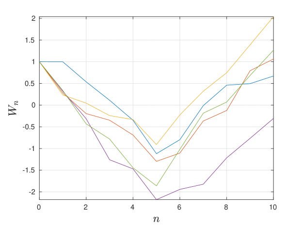
Figure 1: Trajectories of $(W_{n})_{n\in\mathbb{N}}$ with one local minimum at $n=5$ ($\overline{s}=1$, $h=1$).

Note that the conditional distribution of $(W_{1},\ldots,W_{l})$ given $\bigcap_{i=1}^{j}\{\xi_{i}<1/2\}$ and $\bigcap_{i=j+1}^{l}\{\xi_{i}\geq 1/2\}$ coincides with the distribution of $(W^{\prime}_{1},\ldots,W^{\prime}_{l})$, where

$$W^{\prime}_{m}:=\overline{s}-h\sum_{i=1}^{\min(j,m)}\xi_{i}+h\sum_{i=j+1}^{m}\xi_{i},\,\,1\leq m\leq l$$

with the convention that empty sums are defined to be zero.

Using this, and that $B\subset\mathcal{U}=(-\infty,0)\times(-\infty,\underline{\theta})\times(0,M]\times(\overline{\theta},\overline{\theta}+M)\times(\mathbb{N}\setminus\{0\})$, we can write

$$\mathbb{P} \left(U_{1}^{W}\in B,\,W_{j}<\underline{\theta}\leq W_{j-1},\,W_{l-1}\leq\overline{\theta}<W_{l}\middle|\,\bigcap_{i=1}^{j}\{\xi_{i}<1/2\},\,\bigcap_{i=j+1}^{l}\{\xi_{i}\geq 1/2\}\right)=$$

$$=\mathbb{P}\left((-h\xi_{j},W^{\prime}_{j},h\xi_{l},W^{\prime}_{l},l-j)\in B,\,\,\underline{\theta}\leq W^{\prime}_{j-1},\,W^{\prime}_{l-1}\leq\overline{\theta}\right)$$

$$=\int_{0}^{1}\int_{0}^{1}\int_{0}^{\infty}\int_{0}^{\infty}\mathds{1}_{(-hw,\overline{s}-hu-hw,hz,\overline{s}-hu-hw+hv+hz,l-j)\in B}\times$$

$$\times\mathds{1}_{\underline{\theta}\leq\overline{s}-hu}\times\mathds{1}_{\overline{s}-hu-hw+hv\leq\overline{\theta}}\times f_{j-1}(u)\times f_{l-1-j}(v)\,\mathrm{d}u\mathrm{d}v\mathrm{d}w\mathrm{d}z$$

where for $m\in\mathbb{N}_{+}$, $f_{m}:[0,\infty)\to[0,\infty)$ stands for the probability density function of the sum of $m$ independent random variables each having a uniform distribution on $[0,1]$. Now, we can evaluate the quadruple integral using the substitution $x_{1}=-hw$, $x_{2}=\overline{s}-hu-hw$, $x_{3}=hz$, $x_{4}=\overline{s}-hu-hw+hv+hz$, and thus we have

$$\int_{0}^{1}\int_{0}^{1}\int_{0}^{\infty}\int_{0}^{\infty}\mathds{1}_{(-hw,\overline{s}-hu-hw,hz,\overline{s}-hu-hw+hv+hz,l-j)\in B}\times$$

$$\times\mathds{1}_{\underline{\theta}\leq\overline{s}-hu}\times\mathds{1}_{\overline{s}-hu-hw+hv\leq\overline{\theta}}\times f_{j-1}(u)f_{l-1-j}(v)\,\mathrm{d}u\mathrm{d}v\mathrm{d}w\mathrm{d}z=$$

$$=\frac{1}{h^{4}}\int_{\overline{\theta}}^{\overline{\theta}+M}\int_{0}^{h}\int_{-\infty}^{\underline{\theta}}\int_{-h}^{0}\mathds{1}_{(x_{1},x_{2},x_{3},x_{4},l-j)\in B}\times\mathds{1}_{\underline{\theta}\leq x_{2}-x_{1}}\times\mathds{1}_{x_{4}-x_{3}\leq\overline{\theta}}\times$$

$$\times f_{j-1}\left(\frac{\overline{s}-(x_{2}-x_{1})}{h}\right)\times f_{l-1-j}\left(\frac{x_{4}-x_{3}-x_{2}}{h}\right)\,\,\mathrm{d}x_{1}\mathrm{d}x_{2}\mathrm{d}x_{3}\mathrm{d}x_{4}$$

$$=\int_{\mathcal{V}}\mathds{1}_{(\mathbf{x},l-j)\in B}\times g_{\overline{s},j,l-j}(\mathbf{x})\,\lambda(\mathrm{d}\mathbf{x}),$$

where $\mathbf{x}$ is a shorthand notation for $(x_{1},x_{2},x_{3},x_{4})$, $\lambda$ is the Lebesgue measure on $\mathbb{R}^{4}$, and $\mathcal{V}$ is used for $(-\infty,0)\times(-\infty,\underline{\theta})\times(0,M]\times(\overline{\theta},\overline{\theta}+M)$, moreover for $j,m>1$

$$\begin{split}g_{\overline{s},j,m}(\mathbf{x})&=\frac{1}{h^{4}}\mathds{1}_{\underline{\theta}\leq x_{2}-x_{1}}\times\mathds{1}_{x_{4}-x_{3}\leq\overline{\theta}}\times\mathds{1}_{x_{1}\in[-h,0]}\times\mathds{1}_{x_{3}\in[0,h]}\\ &\times f_{j-1}\left(\frac{\overline{s}-(x_{2}-x_{1})}{h}\right)\times f_{m-1}\left(\frac{x_{4}-x_{3}-x_{2}}{h}\right).\end{split}$$ (20)

Substituting this back into (17) and reindexing by $m=l-j$ yields

$\displaystyle\mathbb{P}\left(U_{n+1}\in B,\,L_{n+1}\leq L_{n}+k\mid S_{L_{n}}=\overline{s},\,\tau_{n}=k\right)$ $\displaystyle\geq\sum_{l=2}^{k}\sum_{j=2}^{l-2}\frac{1}{2^{l}}\int_{\mathcal{V}}\mathds{1}_{(\mathbf{x},l-j)\in B}\times g_{\overline{s},j,l-j}(\mathbf{x})\,\lambda(\mathrm{d}\mathbf{x})$ $\displaystyle=\int_{\mathcal{V}}\sum_{m=2}^{k-2}\sum_{j=2}^{k-m}\frac{1}{2^{j+m}}\mathds{1}_{(\mathbf{x},m)\in B}\times g_{\overline{s},j,m}(\mathbf{x})\,\lambda(\mathrm{d}\mathbf{x})$

and thus by (15), we arrive at

$$Q(y,B) \geq\int_{\mathcal{V}}\sum_{k=4}^{\infty}\alpha^{k}(1-\alpha)\sum_{m=2}^{k-2}\sum_{j=2}^{k-m}\frac{1}{2^{j+m}}\mathds{1}_{(\mathbf{x},m)\in B}\times g_{\overline{s},j,m}(\mathbf{x})\,\lambda(\mathrm{d}\mathbf{x})$$

$$=\sum_{m=1}^{\infty}\int_{\mathcal{V}}\mathds{1}_{(\mathbf{x},m)\in B}\times\mathds{1}_{m\geq 2}\times\sum_{k=m+2}^{\infty}\sum_{j=2}^{k-m}\frac{\alpha^{k}(1-\alpha)}{2^{j+m}}g_{\overline{s},j,m}(\mathbf{x})\,\lambda(\mathrm{d}\mathbf{x})$$

$$=\sum_{m=1}^{\infty}\int_{\mathcal{V}}\mathds{1}_{(\mathbf{x},m)\in B}\times\mathds{1}_{m\geq 2}\times\sum_{j=2}^{\infty}\sum_{k=j+m}^{\infty}\frac{\alpha^{k}(1-\alpha)}{2^{j+m}}g_{\overline{s},j,m}(\mathbf{x})\,\lambda(\mathrm{d}\mathbf{x})$$

$$=\int_{B}\mathds{1}_{m\geq 2}\times\sum_{j=2}^{\infty}\frac{\alpha^{j+m}}{2^{j+m}}g_{\overline{s},j,m}(\mathbf{x})\,\lambda(\mathrm{d}\mathbf{x})\otimes\delta(\mathrm{d}m),$$

where $\delta$ is the usual counting measure on $\mathbb{N}$.

Let us observe that on $\mathrm{Supp}(g)\subseteq\mathcal{U}$, $\underline{\theta}\leq x_{2}-x_{1}\leq\underline{\theta}+h$. Now, we fix $0<\tilde{\gamma}<\min\left((\overline{\theta}-\underline{\theta})/h,1\right)$ and consider only $x_{1}$ and $x_{2}$ satisfying $\underline{\theta}\leq x_{2}-x_{1}\leq\underline{\theta}+\tilde{\gamma}h$. Furthermore, since the jumps of $(S_{n})_{n\in\mathbb{N}}$ are bounded from above by $M$, we have $\overline{\theta}<\overline{s}<\overline{\theta}+M$ hence for the argument of $f_{j-1}$ in (20), we get

$$0<\frac{\overline{\theta}-\underline{\theta}}{h}-\tilde{\gamma}\leq\frac{\overline{s}-(x_{2}-x_{1})}{h}\leq\frac{\overline{\theta}-\underline{\theta}}{h}+\frac{M}{h}.$$ (21)

provided that $\underline{\theta}\leq x_{2}-x_{1}\leq\underline{\theta}+\tilde{\gamma}h$.

Introducing $\omega_{j}=\min\{f_{j-1}(t)\mid(\overline{\theta}-\underline{\theta})/h-\tilde{\gamma}\leq t\leq(\overline{\theta}-\underline{\theta})/h+M/h\}$, we arrive at the estimate

$$f_{j-1}\left(\frac{\overline{s}-(x_{2}-x_{1})}{h}\right)\geq\omega_{j}\times\mathds{1}_{\underline{\theta}\leq x_{2}-x_{1}\leq\underline{\theta}+\tilde{\gamma}h}$$

which is uniform in $\overline{s}$, and $\omega_{j}>0$ whenever $j>(\overline{\theta}-\underline{\theta})/h+M/h+1$.

If we put all together, for $C_{h}=\{(\mathbf{x},m)\in\mathcal{U}\mid x_{1}\in[-h,0];\,\underline{\theta}\leq x_{2}-x_{1}\leq\underline{\theta}+\tilde{\gamma}h;\,x_{3}\in[0,h];\,x_{4}-x_{3}\leq\overline{\theta};\,m\geq 2\}$, we obtain

$$Q(y,B)\geq\int_{B\cap C_{h}}\frac{\alpha^{m}}{h^{4}2^{m}}f_{m-1}\left(\frac{x_{4}-x_{3}-x_{2}}{h}\right)\times\sum_{j=2}^{\infty}\frac{\alpha^{j}\omega_{j}}{2^{j}}\,\lambda(\mathrm{d}\mathbf{x})\otimes\delta(\mathrm{d}m),$$

where the right hand-side depends only on $\alpha,M,h,\underline{\theta},\overline{\theta}$, but not on $\overline{s}$ hence (14) holds with

$$\tilde{\kappa}(B)=\int_{B\cap C_{h}}\frac{\alpha^{m}}{h^{4}2^{m}}f_{m-1}\left(\frac{x_{4}-x_{3}-x_{2}}{h}\right)\times\sum_{j=2}^{\infty}\frac{\alpha^{j}\omega_{j}}{2^{j}}\,\lambda(\mathrm{d}\mathbf{x})\otimes\delta(\mathrm{d}m)$$ (22)

which is obviously a non-zero Borel measure on $\mathcal{B}(\mathcal{U})$.

To sum up, we showed that the chain $(U_{n})_{n\geq 1}$ satisfies the uniform minorization condition (14), and thus by Theorem 16.2.2 in [12], there exist a probability measure, independent of $(S_{0},X_{0})$, such that $\mathrm{Law}(U_{n})\to\upsilon$ in total variation. Moreover, by Theorem 17.0.1 in [12], for bounded measurable functionals of $U_{n}$ the law of large numbers holds as it is stated in Theorem 2.6. (Actually, even a central limit theorem could be established.) This completes the proof. ∎

Proof of Theorem 4.1.

The idea of the proof is similar to that of Theorem 2.6, but the details are somewhat simpler. We only sketch the main steps.

We consider the process $Z_{n}=(X_{L_{n}},S_{L_{n}})$, $n>1$ which is obviously a time-homogeneous Markov chain on the state space $\triangle:=\{(x,s)\in(0,M]^{2}\mid x\geq s\}$. In what follows, we prove that chain $(Z_{n})_{n>1}$ satisfies a minorization condition similar to (14) in the proof of Theorem 2.6. More precisely, we aim to show that there exist a non-zero Borel measure $\beta:\mathcal{B}(\triangle)\to[0,\infty)$ such that for all $z\in\triangle$ and $A\in\mathcal{B}(\triangle)$,

$$Q(z,A)\geq\beta(A),$$ (23)

where $Q:\triangle\times\mathcal{B}(\triangle)\to[0,1]$ is the transition kernel of the chain $(Z_{n})_{n\in\mathbb{N}}$.

Let $(\xi_{n})_{n\in\mathbb{N}}$, $(\eta_{n})_{n\in\mathbb{N}}$, and $(\tau_{n})_{n\in\mathbb{N}}$ be as in the the proof of Theorem 2.6. For $z=(\overline{x},\overline{s})\in\triangle$ and $A\in\mathcal{B}(\triangle)$ arbitrary and fixed, by the tower rule, we have

$$\begin{split}Q(z,A)&=\mathbb{P}\left(Z_{n+1}\in A\mid Z_{n}=z\right)=\sum_{k=0}^{\infty}\mathbb{P}\left(Z_{n+1}\in A\mid Z_{n}=z,\,\tau_{n}=k\right)\alpha^{k}(1-\alpha)\\ &\geq\sum_{k=2}^{\infty}\sum_{l=2}^{k}\mathbb{P}\left(Z_{n+1}\in A,\,L_{n+1}=L_{n}+l\mid S_{L_{n}}=\overline{s},\,\tau_{n}=k\right)\alpha^{k}(1-\alpha),\end{split}$$ (24)

where we applied the same principles as in the derivation of (15).

Again by introducing the auxiliary random walk $W_{n}=\overline{s}+h\sum_{j=1}^{n}(2\xi_{j}-1)$, and the associated quantities $L_{n}^{W}$, $Z_{n}^{W}=(h(2\xi_{L_{n}^{W}}-1),W_{L_{n}^{W}})$, $n\in\mathbb{N}$, where $L_{0}^{W}:=0$ and for $n\in\mathbb{N}$, $L_{n+1}^{W}:=\inf\{k>L_{n}^{W}\mid W_{k-1}\leq 0<W_{k}\}$, for fixed $2\leq l\leq k$, we can write

$$\begin{split}&\mathbb{P}\left(Z_{n+1}\in A,\,L_{n+1}=L_{n}+l\mid S_{L_{n}}=\overline{s},\,\tau_{n}=k\right)=\mathbb{P}(Z_{1}^{W}\in A,\,L_{1}^{W}=l)\\ &=\frac{1}{2^{l}}\mathbb{P}\left((h(2\xi_{l}-1),W_{l})\in A,\,W_{l-1}\leq 0<W_{l}\middle|\,\bigcap_{i=1}^{l-1}\{\xi_{i}<1/2\},\,\{\xi_{l}\geq 1/2\}\right)\end{split}$$ (25)

where similarly to (19), we have taken into account trajectories decreasing in $l-1>0$ steps and increasing only in the $l$-th step. For the conditional probability, we have

$$\mathbb{P} \left((h(2\xi_{l}-1),W_{l})\in A,\,W_{l-1}\leq 0<W_{l}\middle|\,\bigcap_{i=1}^{l-1}\{\xi_{i}<1/2\},\,\{\xi_{l}\geq 1/2\}\right)=$$

$$=\int_{0}^{1}\int_{0}^{\infty}\mathds{1}_{(hv,\overline{s}-hu+hv)\in A}\times\mathds{1}_{\overline{s}-hu\leq 0}\times f_{l-1}(u)\mathrm{d}u\mathrm{d}v$$

$$=\frac{1}{h^{2}}\int_{0}^{h}\int_{0}^{x_{1}}\mathds{1}_{(x_{1},x_{2})\in A}\times f_{l-1}\left(\frac{\overline{s}-(x_{2}-x_{1})}{h}\right)\mathrm{d}x_{2}\mathrm{d}x_{1}$$

$$=\int_{(0,h]^{2}\cap A}f_{l-1}\left(\frac{\overline{s}-(x_{2}-x_{1})}{h}\right)\,\lambda(\mathrm{d}\mathbf{x})$$

where $f_{m}:[0,\infty)\to[0,\infty)$ is the probability density function of the sum of $m\geq 1$ independent random variables each having a uniform distribution on $[0,1]$, $\mathbf{x}=(x_{1},x_{2})$, and $\lambda$ denotes the Lebesgue measure on $\mathbb{R}^{2}$.

Notice that if $(x_{1},x_{2})\in(0,h]\cap\triangle$ then $0\leq x_{1}-x_{2}\leq\min(M,h)$, moreover $0<\overline{s}\leq M$ hence we have $0\leq(\overline{s}-(x_{2}-x_{1}))/h\leq M/h+\min(M/h,1)$, and thus we obtain

$$f_{l-1}\left(\frac{\overline{s}-(x_{2}-x_{1})}{h}\right)\geq\omega^{\prime}_{l}\times\mathds{1}_{\tilde{\gamma}^{\prime}\min(M,h)\leq x_{1}-x_{2}},$$ (26)

where $\tilde{\gamma}^{\prime}$ can be any fixed number in $(0,1)$, and $\omega_{l}^{\prime}=\inf\{f_{l-1}(t)\mid\tilde{\gamma}^{\prime}\min(M/h,1)\leq t\leq M/h+\min(M/h,1)\}$ that is a positive number not depending on $\overline{s}$ whenever $l>M/h+1$.

If we put all together, we obtain the following lower estimate

$$Q(z,A) \geq\int_{(0,h]^{2}\cap A}\sum_{k=2}^{\infty}\sum_{l=2}^{k}\frac{\alpha^{k}(1-\alpha)}{2^{l}}\omega^{\prime}_{l}\times\mathds{1}_{\tilde{\gamma}^{\prime}\min(M,h)\leq x_{1}-x_{2}}\,\lambda(\mathrm{d}\mathbf{x})$$

$$=\int_{(0,h]^{2}\cap A}\mathds{1}_{\tilde{\gamma}^{\prime}\min(M,h)\leq x_{1}-x_{2}}\times\sum_{l=2}^{\infty}\frac{\alpha^{l}\omega^{\prime}_{l}}{2^{l}}\,\lambda(\mathrm{d}\mathbf{x}),$$

where the right hand-side depends only on $\alpha,M,h$ and the choice of $\tilde{\gamma}^{\prime}\in(0,1)$, but not depends on $z$, moreover

$$\mathcal{B}(\triangle)\ni A\mapsto\beta(A):=\int_{(0,h]^{2}\cap A}\mathds{1}_{\tilde{\gamma}^{\prime}\min(M,h)\leq x_{1}-x_{2}}\times\sum_{l=2}^{\infty}\frac{\alpha^{l}\omega^{\prime}_{l}}{2^{l}}\,\lambda(\mathrm{d}\mathbf{x})$$

defines a non-zeros Borel measure on $\mathcal{B}(\triangle)$, and thus (23) holds with this $\beta$.

To sum up, we proved that the chain $(Z_{n})_{n\in\mathbb{N}}$ satisfies the uniform minorization condition, and thus it admits a unique invariant probability measure $\pi$ such that $\mathrm{Law}(Z_{n})\to\pi$ at a geometric rate in total variation as $n\to\infty$ (See for example Lemma 18.2.7 and Theorem 18.2.4 in [9]) which completes the proof of Theorem 4.1.

∎

Remark 5.2.

We explain a seemingly innocuous but actually powerful extension of some of the arguments above. Let $X_{t}$ be a time inhomogeneous Markov chain with kernels $P_{n}$, $n\geq 1$ such that

$$P(X_{n+1}\in A|X_{n}=x)=P_{n+1}(x,A),\ x\in\mathcal{X},\ A\in\mathcal{B}(\mathbb{R}),\ n\in\mathbb{N}.$$

Let Assumption 2.1 hold for each $P_{n}$, $n\in\mathbb{N}$ (with the same $\alpha,h$) and let Assumption 2.3 hold for each $P_{n}$. In this case, $U_{t}$, $t\geq 2$ will be a time-inhomogeneous Markov chain and repeating the argument of the proof for Theorem 2.6 establishes the existence of a probability $\tilde{\kappa}$ such that $Q_{n}(x,A)\geq\tilde{\kappa}(A)$, $x\in\mathcal{U}$, $A\in\mathcal{B}(\mathcal{U})$, $n\geq 3$, where $Q_{n+1}(x,A)=P(U_{n+1}\in A|U_{n}=x)$ is the transition kernel of $U$.

Remark 5.3.

One could treat certain stochastic volatility-type models where $X_{t}=\sigma_{t}\varepsilon_{t}$ with $\varepsilon_{t}$ i.i.d. and $\sigma_{t}$ a Markov process. In this case $X_{t}$ is not Markovian but the pair $(X_{t},\sigma_{t})$ is. An extension to even more general non-Markovian $X_{t}$ also seems possible. We do not pursue these generalizations here.

6 Conclusions and future work

It would be desirable to remove the (one-sided) boundedness assumption on the state space of $X_{t}$ and relax the minorization condition (2) to some kind of local minorization. Due to the rather complicated dynamics of $U_{t}$ such extensions do not appear to be straightforward at all.

Removing the boundedness hypothesis on $u,p$ in Section 3 would also be desirable but looks challenging.

Replacing the constant drift $\mu$ by a functional of $X_{t}$ would also significantly extend the family of models in consideration.

An adaptive optimization of the thresholds $\underline{\theta},\overline{\theta}$ could be performed using the Kiefer-Wolfowitz algorithm, as proposed in Section 6 of [17]. There are a number of technical conditions (e.g. mixing properties, smoothness of the laws) that need to be checked for applying [17] but the ergodic properties established in this article strongly suggest that this programme indeed can be carried out.

Extensions to non-Markovian stochastic volatility models (see [7, 10]) seem feasible but require further technicalities.

References

- [1] Mean reversion trading: Is it a profitable strategy? https://www.warriortrading.com/mean-reversion/, Retrieved on 24th November 2021.
- [2] Mean reversion trading strategy with a sneaky secret. https://tradingstrategyguides.com/mean-reversion-trading-strategy/, Retrieved on 24th November 2021.
- [3] What is mean reversion trading strategy. https://tradergav.com/what-is-mean-reversion-trading-strategy/, Retrieved on 24th November 2021.
- [4] R. Bhattacharya and M. Majumdar. On a theorem of Dubins and Freedman. J. Theor. Prob., 12:1067–1087, 1999.
- [5] R. Bhattacharya and E. Waymire. Stochastic Processes with Applications. Wiley & Sons, New York, 1990.
- [6] Á. Cartea, S. Jaimungal and J. Ricci. Buy low sell high: a high frequency trading perspective. SIAM J. Financ. Math. 5:415–444, 2014.
- [7] F. Comte and É. Renault. Long memory in continuous-time stochastic volatility models. Math. Finance, 8:291–323, 1998.
- [8] M. Dai, H. Jin, Y. Zhong, X. Y. Zhou. Buy low and sell high. In: Chiarella, C., Novikov, A. (eds.) Contemporary Quantitative Finance: Essays in Honour of Eckhard Platen, 317–333, Springer, 2010.
- [9] R. Douc, E. Moulines, P. Priouret and Ph. Soulier. Markov chains. Operation research and financial engineering. Springer, 2018.
- [10] J. Gatheral, T. Jaisson, and M. Rosenbaum. Volatility is rough. Quantitative Finance, 18:933–949, 2018.
- [11] T. S. Leung and X. Li. Optimal Mean Reversion Trading: Mathematical Analysis and Practical Applications. World Scientific, Singapore, 2015.
- [12] S. P. Meyn and R. L. Tweedie. Markov chains and stochastic stability. Springer-Verlag, 1993.
- [13] A. Mijatović and V. Vysotsky. Stability of overshoots of zero mean random walks. Electronic Journal of Probability, 25(none):1–22, 2020.
- [14] A. Mijatović and V. Vysotsky. Stationary entrance Markov chains, inducing, and level-crossings of random walks. Preprint, arXiv:1808.05010, 2020.
- [15] J. Neveu. Discrete-parameter martingales. North-Holland, 1975.
- [16] H. Pham. Continuous-time Stochastic Control and Optimization with Financial Applications, Springer, 2008.
- [17] M. Rásonyi and K. Tikosi. Convergence of the Kiefer-Wolfowitz algorithm in the presence of discontinuities. To appear in Advances in Applied Probability, 2022. arXiv:2002.04832
- [18] A. Shiryaev, Z. Xu, and X. Y. Zhou. Thou Shalt Buy and Hold. Quantitative Finance 8:765–776.
- [19] Q. S. Song, G. Yin, and Q. Zhang. Stochastic Optimization Methods for Buying-Low-and-Selling-High Strategies. Stochastic Analysis and Applications, 27:523–542, 2009.
- [20] M. Zervos, T. C. Johnson, F. Alazemi. Buy-low and sell-high investment strategies. Math. Finance, 23:560–578, 2013.
- [21] H. Zhang, Q. Zhang. Trading a mean-reverting asset: buy low and sell high. Automatica 44:1511–1518, 2008.
- [22] Q. Zhang. Stock Trading: an Optimal Selling Rule. SIAM Journal on Control and Optimization, 40:64–87, 2001.
- [23] C. Zhuang. Stochastic approximation methods and applications in financial optimization problems. PhD thesis, University of Georgia, 2008.