The basics and applications of the tempered Lefschetz thimble method for the numerical sign problem

Abstract

The numerical sign problem has long been a major obstacle to first-principles calculations in various important fields of physics. We report that the recently proposed algorithm, tempered Lefschetz thimble method (TLTM), and its worldvolume extension (WV-TLTM) can be a promising solution in its trustability and versatility.

1 Introduction

The Monte Carlo (MC) method has been intensively used for first-principles calculations of the strong interaction, based on the lattice QCD. However, for the computation at finite density, the bosonized action becomes complex-valued, and one is forced to make a MC estimation of a highly oscillatory integral. This gives rise to an extraordinarily high computational cost, exponentially increasing with the degrees of freedom (DOF). Such a problem is called the sign problem, and has been a major obstacle to first-principles calculation in various important fields of physics. Typical examples are, in addition to the aforementioned finite density QCD [1], the $\theta$-vacuum with finite $\theta$, the Quantum Monte Carlo calculation of strongly correlated electron systems and frustrated spin systems, and the real-time dynamics of quantum fields. Among various approaches proposed so far towards solving the sign problem, in this talk we concentrate on the Lefschetz thimble method [3, 4, 5, 6, 7, 8, 9, 10, 11], especially its tempered version [6] as well as the worldvolume extension [10].

In section 2, we explain the basics of the Lefschetz thimble method and point out that it suffers from the dilemma between the sign problem and the ergodicity problem. Section 3 describes our solution, the tempered Lefschetz thimble method (TLTM) [6], and its improved version, the worldvolume tempered Lefschetz thimble method (WV-TLTM) [10]. The WV-TLTM is discussed in more detail in the contribution [12] together with its statistical analysis method. In section 4, we exemplify the effectiveness of the (WV-)TLTM by its successful application to various models. Section 5 is devoted to conclusion and outlook.

Note: Some part of the presentation in this proceedings has a substantial overlap with a contribution to CCP2021 [13].

2 Lefschetz thimble method

Our aim is to numerically estimate the expectation values of observables defined by the path integral

$$\langle\mathcal{O}(x)\rangle\equiv\frac{\int_{{\mathbb{R}}^{N}}dx\,e^{-S(x)}\,\mathcal{O}(x)}{\int_{{\mathbb{R}}^{N}}dx\,e^{-S(x)}},$$ (1)

where $x=(x^{i})\in{\mathbb{R}}^{N}$ is the dynamical variable, $S(x)$ the action, $dx\equiv\prod_{i=1}^{N}dx^{i}$ the measure of the path integral, and $\mathcal{O}(x)$ an observable of interest. When the action $S(x)$ is complex-valued, the Boltzmann weight $e^{-S(x)}/Z$ ($Z=\int dx\,e^{-S(x)}$) is not a positive semidefinite function, and thus cannot be regarded as a probability distribution. The simplest and most naive MC method for a complex action $S(x)$ is the reweighting method, where we use the real part ${\rm Re}\,S(x)$ for a new Boltzmann weight, and treat the phase factor $e^{-i\,{\rm Im}\,S(x)}$ as a part of observable:

$$\langle\mathcal{O}(x)\rangle=\frac{\langle e^{-i\,{\rm Im}\,S(x)}\,\mathcal{O}(x)\rangle_{\rm rewt}}{\langle e^{-i\,{\rm Im}\,S(x)}\rangle_{\rm rewt}}\quad\Bigl{(}\langle f(x)\rangle_{\rm rewt}\equiv\frac{\int dx\,e^{-{\rm Re}\,S(x)}\,f(x)}{\int dx\,e^{-{\rm Re}\,S(x)}}\Bigr{)}.$$ (2)

However, because of the highly oscillatory behavior of $e^{-i\,{\rm Im}\,S(x)}$ at large degrees of freedom (i.e., when $N\gg 1$), Eq. (2) becomes a ratio of very small quantities even when $\mathcal{O}(x)$ is an operator of $O(1)$:

$$\langle\mathcal{O}(x)\rangle=\frac{\langle e^{-i\,{\rm Im}\,S(x)}\,\mathcal{O}(x)\rangle_{\rm rewt}}{\langle e^{-i\,{\rm Im}\,S(x)}\rangle_{\rm rewt}}=\frac{e^{-O(N)}}{e^{-O(N)}}\,\bigl{(}\,=O(1)\bigr{)}.$$ (3)

Of course, this does not cause a problem if we can evaluate both the numerator and the denominator precisely. However, in the MC calculations they are estimated separately from sample averages, and thus are necessarily accompanied by statistical errors, leading to an estimate of the form

$$\langle\mathcal{O}(x)\rangle\approx\frac{e^{-O(N)}\pm O(1/\sqrt{N_{\rm conf}})}{e^{-O(N)}\pm O(1/\sqrt{N_{\rm conf}})}.$$ (4)

Thus, in order for the statistical errors to be smaller than the main parts, we need the inequality $\sqrt{N_{\rm conf}}\lesssim e^{-O(N)}$, which means that the sample size must be exponentially large: $N_{\rm conf}\gtrsim e^{O(N)}.$ This is the sign problem.

In the Lefschetz thimble method, we complexify the dynamical variable from $x=(x^{i})\in{\mathbb{R}}^{N}$ to $z=(z^{i})=x+iy\in{\mathbb{C}}^{N}$. We make an assumption (which usually holds for systems of interest) that $e^{-S(z)}$ and $e^{-S(z)}\,\mathcal{O}(z)$ are both entire functions over ${\mathbb{C}}^{N}$. Then, due to Cauchy’s theorem, the integrals do not change under continuous deformations of integration surface (see the left panel of Fig. 1):

$$\langle\mathcal{O}(x)\rangle=\frac{\int_{{\mathbb{R}}^{N}}dx\,e^{-S(x)}\,\mathcal{O}(x)}{\int_{{\mathbb{R}}^{N}}dx\,e^{-S(x)}}=\frac{\int_{\Sigma}dz\,e^{-S(z)}\,\mathcal{O}(z)}{\int_{\Sigma}dz\,e^{-S(z)}}.$$ (5)

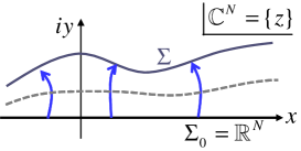
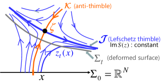
Figure 1: Deformation of integration surface.

Thus, even when the sign problem is very severe on $\Sigma_{0}={\mathbb{R}}^{N}$ due to the highly oscillatory phase factor $e^{-i\,{\rm Im}\,S(x)}$, the sign problem will be significantly reduced if the deformed integration surface $\Sigma$ can be chosen such that ${\rm Im}\,S(z)$ is almost constant on $\Sigma$.

The prescription for such a deformation is the following anti-holomorphic gradient flow (see the right panel of Fig. 1):

$$\dot{z}_{t}=[\partial S(z_{t})]^{\ast},\quad z_{t=0}=x,$$ (6)

which defines a map from $x\in\Sigma_{0}={\mathbb{R}}^{N}$ to $z=z_{t}(x)\in{\mathbb{C}}^{N}$. We denote the deformed surface at flow time $t$ by $\Sigma_{t}\,(\equiv\{z_{t}(x)\,|\,x\in{\mathbb{R}}^{N}\})$. From the inequality

$$[S(z_{t})]^{\cdot}=\partial S(z_{t})\cdot\dot{z}_{t}=|\partial S(z_{t})|^{2}\geq 0,$$ (7)

we see that

• $[{\rm Re}\,S(z_{t})]^{\cdot}\geq 0$, i.e., ${\rm Re}\,S(z_{t})$ always increases along the flow except at critical points (points where the gradient of the action vanishes),

• $[{\rm Im}\,S(z_{t})]^{\cdot}=0$, i.e., ${\rm Im}\,S(z_{t})$ is constant along the flow.

Associated with a critical point $\zeta$, we define the corresponding Lefschetz thimble $\mathcal{J}$ as a union of orbits flowing out of $\zeta$,

$$\mathcal{J}\equiv\bigl{\{}z\,\bigl{|}\,\lim_{t\to-\infty}z_{t}(z)=\zeta\bigr{\}}.$$ (8)

Due to the property (b), ${\rm Im}\,S(z)$ is constant on $\mathcal{J}$, ${\rm Im}\,S(z)={\rm Im}\,S(\zeta)$ $(z\in\mathcal{J})$. Thus, when $\Sigma_{t}$ approaches a single Lefschetz thimble in the large flow time limit, we expect that the integration on $\Sigma_{t}$ becomes free from the sign problem by taking the flow time $t$ to be sufficiently large.

The disappearance of the sign problem actually goes as follows. When we make a reweighting at flow time $t$, the main parts in the numerator and the denominator turn out to be of order $e^{-e^{-\lambda t}\,O(N)}$ with $\lambda$ a typical singular value of the matrix $\partial_{i}\partial_{j}S(\zeta)$, so that the expectation value is estimated as

$$\langle\mathcal{O}(x)\rangle=\frac{\langle e^{i\theta(z)}\mathcal{O}(z)\rangle_{\Sigma_{t}}}{\langle e^{i\theta(z)}\rangle_{\Sigma_{t}}}\approx\frac{e^{-e^{-\lambda t}\,O(N)}\pm O(1/\sqrt{N_{\rm conf}})}{e^{-e^{-\lambda t}\,O(N)}\pm O(1/\sqrt{N_{\rm conf}})}.$$ (9)

Therefore, if we take the flow time $t$ to be sufficiently large so as to satisfy $e^{\lambda t}=O(N)$, the main parts become $O(1)$, and thus we no longer need a huge size of sample.

So far, so good. However, when multiple thimbles are relevant to estimation, there generically arises another problem at large flow times, the ergodicity problem. Figure 2 is a sketch of the deformation of integration surface for the case $e^{-S(x)}=e^{-\beta x^{2}/2}\,(x-i)^{\beta}$.

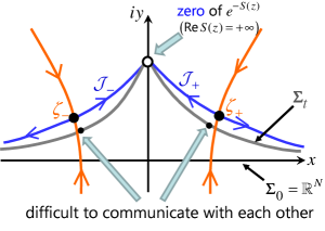
Figure 2: Ergodicity problem caused by a zero of $e^{-S(z)}$.

There, in addition to two critical points at $\zeta_{\pm}=\pm\sqrt{3}/2+i/2$ and the corresponding thimbles $\mathcal{J}_{\pm}$, we have a zero of $e^{-S(z)}$ at $z=i$, which behaves as an infinitely high potential barrier on $\Sigma_{t}$. Thus, in a Markov chain MC simulation, the configuration space $\Sigma_{t}$ is not well explored due to this potential barrier, and we eventually need a large computation time to realize global equilibrium. This is the ergodicity problem, which is believed to remain after taking the continuum limit [14].

As a solution to this ergodicity problem, it was made a very interesting proposal in Ref. [5] to employ a flow time which is sufficiently large so as to resolve the sign problem but at the same time is not too large so as to avoid the ergodicity problem. However, explicit simulations show that in many important cases the sign problem becomes mild only after the deformed surface reaches a zero, and furthermore, there is no reason to be capable of finding such a nice flow time for a system at large degrees of freedom, for which the flows around critical points and zeros are complicated.

The tempered Lefschetz thimble method (TLTM) [6] was proposed to resolve both the sign problem (severe at small flow times) and the ergodicity problem (severe at large flow times) simultaneously by implementing the tempering algorithm [15, 16, 17, 18] to the Lefschetz thimble method.

3 Tempered Lefschetz thimble method and its worldvolume extension

3.1 Tempered Lefschetz thimble method

The basic algorithm of the TLTM is as follows [6] (see the left panel of Fig. 3):

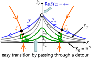
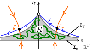
Figure 3: Configuration spaces of TLTM (left) and WV-TLTM (right).

• We set the target flow time $T$ which is large enough to resolve the sign problem.

• We introduce replicas in between the original integration surface $\Sigma_{0}={\mathbb{R}}^{N}$ and the target integration surface $\Sigma_{T}$: $\{\Sigma_{t_{0}=0},\,\Sigma_{t_{1}},\,\Sigma_{t_{2}},\ldots,\Sigma_{t_{A}=T}\}.$

• We construct a Markov chain which consists of (i) transitions on each surface $\Sigma_{t_{a}}$ and (ii) exchanges of configurations between adjacent replicas $\Sigma_{t_{a}}$ and $\Sigma_{t_{a+1}}$. The Markov chain is designed so that the equilibrium distribution on the extended configuration space ${\mathbb{R}}^{N}\times\mathcal{A}=\{(x,t_{a})\,|\,x\in{\mathbb{R}}^{N},\,a=1,\ldots,A\}$ is given by $\rho(x,t_{a})\propto e^{-S(z_{t_{a}}(x))}\,|\det J_{t_{a}}(x)|$, where $J_{t}(x)=\partial z_{t}(x)/\partial x$ is the Jacobian matrix of the flow.

• After equilibration, we estimate observables with a subsample from the replica at $t_{A}=T$.

Note that estimates from replicas at large flow times (where the sign problem is reduced) must agree within statistical errors due to Cauchy’s theorem. This observation enables us to enhance the precision of estimate by using the $\chi^{2}$ fit with a constant as the fitting function [8].

3.2 Worldvolume Tempered Lefschetz Thimble Method (WV-TLTM)

Recall that in the original TLTM [6], we temper a system with the flow time introducing a finite discrete set of replicas $\{\Sigma_{t_{0}},\Sigma_{t_{1}},\ldots,\Sigma_{t_{A}}\}$. The advantage of this method over others is its versatility. In fact, the method can in principle be applied to any systems once the problem is defined in a path integral form over continuous variables. A drawback is its high computational cost at large DOF. In fact, the algorithm requires the computation of $\det J_{t}(x)$ in generating a configuration, whose cost is $O(N^{3})$. This cost is further multiplied by the additional cost due to the implementation of the tempering, which is expected to be $O(N^{0-1})$.

To overcome this drawback, the worldvolume tempered Lefschetz thimble method (WV-TLTM) was invented in Ref. [10], where HMC updates are performed on a continuous accumulation of integration surfaces, $\mathcal{R}\equiv\bigcup_{0\leq t\leq T}\Sigma_{t}$ (see the right panel of Fig. 3). We call this region $\mathcal{R}$ the worldvolume of integration surface. This WV-TLTM significantly reduces the numerical cost at large DOF, keeping the aforementioned advantages intact. In fact, in the WV-TLTM,

• we no longer need to worry about the acceptance rate in the exchange process,

• we no longer need to compute the Jacobian of the flow in generating a configuration,

• we can move configurations largely due to the use of the HMC algorithm.

The fundamental idea behind the WV-TLTM is that Cauchy’s theorem allows us to average the denominator and the numerator in Eq. (5) over $t$ with an arbitrary weight $e^{-W(t)}$:

$$\langle\mathcal{O}(x)\rangle =\frac{\int_{\Sigma_{0}}dx\,e^{-S(x)}\,\mathcal{O}(x)}{\int_{\Sigma_{0}}dx\,e^{-S(x)}}=\frac{\int_{\Sigma_{t}}dz_{t}\,e^{-S(z_{t})}\,\mathcal{O}(z_{t})}{\int_{\Sigma_{t}}dz_{t}\,e^{-S(z_{t})}}$$

$$=\frac{\int_{0}^{T}dt\,e^{-W(t)}\,\int_{\Sigma_{t}}dz_{t}\,e^{-S(z_{t})}\,\mathcal{O}(z_{t})}{\int_{0}^{T}dt\,e^{-W(t)}\,\int_{\Sigma_{t}}dz_{t}\,e^{-S(z_{t})}}=\frac{\int_{\mathcal{R}}dt\,dz_{t}\,e^{-W(t)-S(z_{t})}\,\mathcal{O}(z_{t})}{\int_{\mathcal{R}}dt\,dz_{t}\,e^{-W(t)-S(z_{t})}}.$$ (10)

The final expression does take a form of path integral over the region $\mathcal{R}$, and further can be rewritten to a ratio of reweighted integrals with a potential $V(z)\equiv{\rm Re}\,S(z)+W(t(z))$ [$t(z)$ is the flow time at $z\in\mathcal{R}$]. As can be seen from the absence of the Jacobian in $V(z)$, the molecular dynamics can be performed without calculating the Jacobian matrix [10] (see also the contribution [12]). Although $e^{-W(t)}$ can be an arbitrary function of $t$ in principle, practically it is chosen such that the appearance ratios at different flow times $t$ are almost the same so as to ensure the region to be fully explored.

4 Applications

The TLTM has been successfully applied to various models, including

• $(0+1)$-dimensional massive Thirring model [6]

• two-dimensional Hubbard model [8, 9]

• a chiral random matrix model (Stephanov model) [10]

• antiferromagnetic Ising model on a triangular lattice [M. Fukuma and N. Matsumoto, talk at JPS meeting 2020]

Below we discuss the application of WV-TLTM [10] to the Stephanov model [19].

The grand partition function of finite density QCD takes the form

$$Z_{\rm QCD}=\int[dA_{\mu}]\,e^{(1/2g^{2})\int{\rm tr}\,F_{\mu\nu}^{2}}\,{\rm Det}\,\left(\begin{array}[]{cc}m&\sigma_{\mu}(\partial_{\mu}+A_{\mu})+\mu\\ \sigma_{\mu}^{\dagger}(\partial_{\mu}+A_{\mu})+\mu&m\end{array}\right).$$ (13)

The Stephanov model is obtained by replacing the gauge-field degrees of freedom with a complex matrix, and takes the following form at zero temperature:

$$Z_{\rm Steph}\equiv\int d^{2}W\,e^{-n\,{\rm tr}\,W^{\dagger}W}\,{\rm det}\,\left(\begin{array}[]{cc}m&iW+\mu\\ iW^{\dagger}+\mu&m\end{array}\right).$$ (16)

Here, $W=(W_{ij}=X_{ij}+iY_{ij})$ is an $n\times n$ complex matrix, and thus the DOF is given by $N=2n^{2}$. This corresponds to the DOF of the gauge field on a lattice, $4L^{4}(N_{c}^{2}-1)$ [$L$ :  linear size of four-dimensional periodic lattice, and $N_{c}$ :  color ($N_{c}=3$ for QCD) ]. This model is regarded as an important benchmark for algorithms towards solving the sign problem, because

• the model well describes the qualitative behavior of finite density QCD in the large $n$ limit,

• the complex Langevin method [20, 21] fails for this model because of the serious wrong convergence problem [22].

Figures 4 and 5 show the estimates of the chiral condensate and the baryon number density obtained with three methods: (i) the naive reweighting method, (ii) the complex Langevin method, and (iii) the WV-TLTM [10].

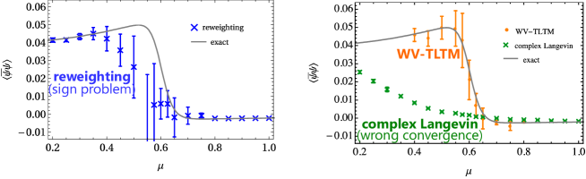
Figure 4: Chiral condensate $\langle\bar{\psi}\psi\rangle\equiv(1/2n)(\partial/\partial m)\ln Z_{\rm Steph}$ [10].

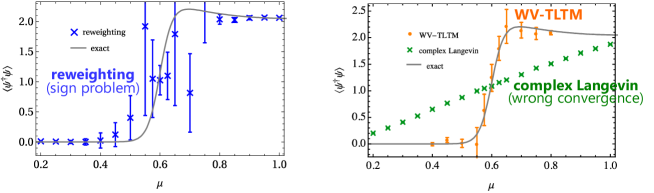
Figure 5: Baryon number density $\langle\psi^{\dagger}\psi\rangle\equiv(1/2n)(\partial/\partial\mu)\ln Z_{\rm Steph}$ [10].

We see that the naive reweighting method fails due to the sign problem, and also that the complex Langevin method gives wrong results with small statistical errors. On the other hand, the WV-TLTM gives correct results agreeing with the exact values. In fact, this is the first (and only at the moment) successful example among the attempts using various methods to reproduce the correct results for the Stephanov model in parameter regions where the sign problem is severe.

5 Conclusion and Outlook

The sign problem has been an obstacle to first-principles calculations in various important fields of physics, and a versatile solution has long been awaited. In this talk, we report that the (WV-)TLTM can be one of the most powerful candidate as a solution.

Our group including the present authors has already started the full-scale application of the WV-TLTM to systems at large DOF, porting the code so as to run on a supercomputer. In parallel with research in this direction, we believe that it is still important to continue developing the algorithm itself for further efficiency at large DOF.

The most important in the future development will be the application to the real-time dynamics of quantum fields. If a MC method is at hand for time-dependent quantum systems, the first-principles calculation will become possible for nonequilibrium systems, such as the very early Universe and heavy ion collision experiments.

References

- [1] J. Guenther, An overview of the QCD phase diagram at finite and , PoS LATTICE2021 (2021) 013
- [2] E. Witten, Analytic Continuation Of Chern-Simons Theory, AMS/IP Stud. Adv. Math. 50 (2011) 347 [1001.2933].
- [3] M. Cristoforetti, F. Di Renzo and L. Scorzato, New approach to the sign problem in quantum field theories: High density QCD on a Lefschetz thimble, Phys. Rev. D 86 (2012) 074506 [1205.3996].
- [4] H. Fujii, D. Honda, M. Kato, Y. Kikukawa, S. Komatsu and T. Sano, Hybrid Monte Carlo on Lefschetz thimbles - A study of the residual sign problem, JHEP 1310 (2013) 147 [1309.4371].
- [5] A. Alexandru, G. Başar, P. F. Bedaque, G. W. Ridgway and N. C. Warrington, Sign problem and Monte Carlo calculations beyond Lefschetz thimbles, JHEP 1605 (2016) 053 [hep-lat/1512.08764].
- [6] M. Fukuma and N. Umeda, Parallel tempering algorithm for integration over Lefschetz thimbles, PTEP 2017 (2017) 073B01 [hep-lat/1703.00861].
- [7] A. Alexandru, G. Başar, P.F. Bedaque and N.C. Warrington, Tempered transitions between thimbles, Phys. Rev. D 96 (2017) 034513 [1703.02414].
- [8] M. Fukuma, N. Matsumoto and N. Umeda, Applying the tempered Lefschetz thimble method to the Hubbard model away from half filling, Phys. Rev. D 100 (2019) 114510 [1906.04243].
- [9] M. Fukuma, N. Matsumoto and N. Umeda, Implementation of the HMC algorithm on the tempered Lefschetz thimble method, 1912.13303.
- [10] M. Fukuma and N. Matsumoto, Worldvolume approach to the tempered Lefschetz thimble method, PTEP 2021 (2021) 023B08 [2012.08468].
- [11] M. Fukuma, N. Matsumoto and Y. Namekawa, Statistical analysis method for the worldvolume hybrid Monte Carlo algorithm, to appear in PTEP [hep-lat/2107.06858].
- [12] M. Fukuma, N. Matsumoto and Y. Namekawa, Worldvolume tempered Lefschetz thimble method and its error estimation, PoS LATTICE2021 (2021) 446.
- [13] M. Fukuma and N. Matsumoto, Tempered Lefschetz thimble method as a solution to the numerical sign problem, contribution to XXXII IUPAP Conference on Computational Physics (2021).
- [14] H. Fujii, S. Kamata and Y. Kikukawa, Lefschetz thimble structure in one-dimensional lattice Thirring model at finite density, JHEP 11 (2015) 078 [erratum: JHEP 02 (2016) 036] [hep-lat/1509.08176].
- [15] E. Marinari and G. Parisi, Simulated tempering: A new Monte Carlo scheme, Europhys. Lett. 19 (1992) 451 [hep-lat/9205018]
- [16] R. H. Swendsen and J.-S. Wang, Replica Monte Carlo Simulation of Spin-Glasses, Phys. Rev. Lett. 57 (1986) 2607.
- [17] C. J. Geyer, Markov Chain Monte Carlo Maximum Likelihood, in Computing Science and Statistics: Proceedings of the 23rd Symposium on the Interface, American Statistical Association, New York, p. 156 (1991).
- [18] K. Hukushima and K. Nemoto, Exchange Monte Carlo method and application to spin glass simulations, J. Phys. Soc. Jpn. 65 (1996) 1604.
- [19] M. A. Stephanov, Random matrix model of QCD at finite density and the nature of the quenched limit, Phys. Rev. Lett. 76 (1996) 4472 [hep-lat/9604003].
- [20] G. Parisi, On complex probabilities, Phys. Lett. B 131 (1983) 393.
- [21] J.R. Klauder, Coherent State Langevin Equations for Canonical Quantum Systems With Applications to the Quantized Hall Effect, Phys. Rev. A 29 (1984) 2036.
- [22] J. Bloch, J. Glesaaen, J. J. M. Verbaarschot and S. Zafeiropoulos, Complex Langevin Simulation of a Random Matrix Model at Nonzero Chemical Potential, JHEP 03 (2018) 015 [1712.07514].