Learning Fair Classifiers with Partially Annotated Group Labels

Abstract

Recently, fairness-aware learning have become increasingly crucial, but most of those methods operate by assuming the availability of fully annotated demographic group labels. We emphasize that such assumption is unrealistic for real-world applications since group label annotations are expensive and can conflict with privacy issues. In this paper, we consider a more practical scenario, dubbed as Algorithmic Group Fairness with the Partially annotated Group labels (Fair-PG). We observe that the existing methods to achieve group fairness perform even worse than the vanilla training, which simply uses full data only with target labels, under Fair-PG. To address this problem, we propose a simple Confidence-based Group Label assignment (CGL) strategy that is readily applicable to any fairness-aware learning method. CGL utilizes an auxiliary group classifier to assign pseudo group labels, where random labels are assigned to low confident samples. We first theoretically show that our method design is better than the vanilla pseudo-labeling strategy in terms of fairness criteria. Then, we empirically show on several benchmark datasets that by combining CGL and the state-of-the-art fairness-aware in-processing methods, the target accuracies and the fairness metrics can be jointly improved compared to the baselines. Furthermore, we convincingly show that CGL enables to naturally augment the given group-labeled dataset with external target label-only datasets so that both accuracy and fairness can be improved. Code is available at https://github.com/naver-ai/cgl_fairness.

1 Introduction

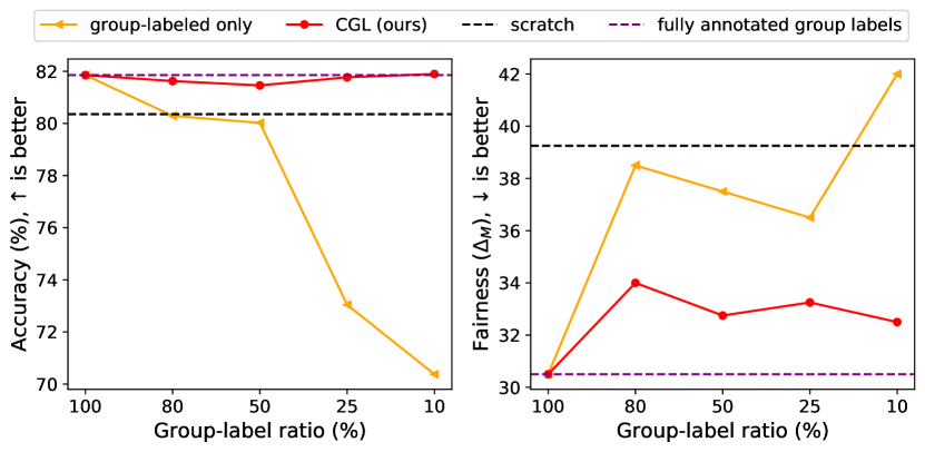
Figure 1: Can fair-training methods still learn fair classifiers when group labels are partially annotated? We note the state-of-the-art fairness fair-training FairHSIC [51] using only the group-labeled subset (yellow) shows worse fairness criterion ($\Delta_{M}$, Eq. 2, lower the better) than the “scratch” (i.e., no consideration of a fairness criteria) in the low group label regime (e.g., 10%) on UTKFace [67]. Our CGL (red), on the other hand, can be potentially applied to any fair-training method, and when it is combined with FairHSIC, both the target accuracy and the fairness criteria are significantly improved for the low group label regime.

Recent advances of machine learning (ML) models have witnessed promising outcomes even in societal applications, such as credit estimation [41], crime assessment systems [9, 36], automatic job interviews [48], face recognition [10, 59], and law enforcement [25]. However, machines are often more inaccurate to a particular group (e.g., darker-skinned females) than other groups (e.g., lighter-skinned males) [10], i.e., machines are discriminatory. To mitigate the issue, fairness-aware learning has recently emerged; a model should not discriminate against any demographic group with sensitive attributes, e.g., age, gender, or race.

Many existing approaches for group fairness [64, 63, 1, 51, 35, 17, 37] utilize two types of labels: target labels, which are task-oriented (e.g., crime assessment) and group labels, which are defined by socially sensitive attribute groups (e.g., ethnicity or gender). Many existing methods for achieving group fairness rely on the group labels to train fair classifiers. For example, many approaches explicitly minimize the statistical parity metrics between groups defined by sensitive attributes. However, in many realistic applications, e.g., computer vision, assuming that all images have sensitive group labels can be unrealistic and make the existing methods impractical. First, in many image datasets, group labels are not explicitly given as in tabular datasets [9, 41, 36] but are defined in high-level semantics, requiring additional expensive human annotations. Secondly, the sensitive attributes are usually personal information protected by laws, such as EU General Data Protection Regulation (GDPR). Hence, in real-world applications, collecting group labels for all data points are impossible without permissions by all users and, furthermore, sensitive attributes cannot be persistently stored but should be expired. Thus, the underlying assumption by the previous fair-training methods, i.e., group labels are fully annotated, can limit their usability in real-world applications.

Contribution.

In this work, we propose and investigate a less explored but very practical problem: Algorithmic Group Fairness with the Partially annotated Group labels (Fair-PG). Many existing fair-training methods for group fairness assume all training samples have group labels, and optimize fairness constraints by the group labeled training samples. In this case, they cannot be directly applied to the Fair-PG problem. We empirically show that the baseline fair-training methods, which operate only on the group-labeled samples, perform even worse than the vanilla “scratch” training that use all the training samples, in terms of fairness when the number of group-labeled samples is small (e.g., 10%) – See Fig. 1. Although there exist a few attempts to achieve algorithmic fairness without demographics labels [32, 44], they do not directly solve the group fairness problem. Also, they do not utilize partially annotated group labels at all, while a small number of labeled data can improve the overall performances. To this end, we propose a simple yet effective strategy for Fair-PG that can be applied to any fair-training methods for group fairness, dubbed as Confidence-based Group Label assignment (CGL). CGL assigns pseudo group labels to group-unlabeled samples using an auxiliary group classifier, if the predictions are sufficiently confident, and random group labels, otherwise.

We provide high-level understandings of how CGL works on the Fair-PG scenario. We theoretically support that (1) the fairness parity computed by our approach approximates the parity of the underlying group label distribution better than the one by the vanilla pseudo-label strategy which totally trusts the predictions of the auxiliary group classifier, (2) assigning a random group label to a data point implies the elimination of the fairness constraint of the sample. In practice, since the existing fair-training methods use a relaxed constraint, CGL can be interpreted as a regularization method for the low confident group-unlabeled samples.

In our experiments, the combination of CGL with state-of-the-art fair-traning methods (e.g., MFD [37], FairHSIC [51] and LBC [35]) has consistently and significantly improved target accuracies as well as fairness parities even under the low group label regime on facial image [67, 46] and tabular [36, 21] datasets. For example, compared to the “group-labeled only” baseline, the combination of CGL and MFD shows +8.23% target accuracy increase and -8.75 disparity of equal opportunity (DEO) decrease on UTKFace [67], when only 10% of data points have group labels. Further extending this result, by augmenting the full UTKFace training set with extra group-unlabeled dataset in [40], we show that CGL can significantly improve the performance of MFD by +0.92% accuracy and -5.5 DEO. This is promising since it shows CGL can improve both the accuracy and fairness of a baseline method by augmenting the training data with target label-only dataset, which is relatively easier to obtain than jointly requiring the group labels.

2 Related Works

Fair-training for group fairness.

There have been various works to tackle fairness problem in machine learning models. At a high level, it can usually be classified into three categories, including 1) individual fairness [22, 62] that aims to treat similar users similarly, 2) group fairness [31] of which goal is to reduce the statistical parity between groups defined by the sensitive attributes, 3) Rawlsian min-max fairness [44, 23, 32] which designs to improve the worst performance among groups. In this paper, we follow the notion of group fairness in arguing the fairness of a model. Many fair-training methods have been developed to achieve group fairness. The fairness methods (for group fairness) can be divided into three categories depending on where the technique for fairness is injected into; pre-processing methods [64, 51, 20] modify a training dataset before learning a model; in-processing [39, 63, 37, 17, 65, 35] methods consider fairness during training time; post-processing methods [3] modify a trained model. However, despite technical advances for achieving group fairness, existing methods for group fairness have not considered the setting in which a part of a training dataset lacks group label (i.e., Fair-PG).

Fairness with imperfect sensitive attributes.

Recently, a few attempts have been proposed to consider algorithmic fairness with imperfect sensitive attributes, e.g., noisy group labels. Chen et al. [14] and Kallus et al. [38] proposed methods for assessing the disparity when only proxy variables (e.g., surname) for the protected variables are given. Meanwhile, several works [60, 2] posed solutions of learning a fair classifier robust to noisy group labels. However, these approaches focus only on noisy group labels, hence they cannot be directly applied to our Fair-PG setting.

There also have been a few works for fair-training without any information of protected attributes. Hashimoto et al. [32] proposed a distributionally robust optimization (DRO) [47] based approach, and Lahoti et al. [44] utilized an adversary to identify regions with high loss and re-weight them. Similarly, there exist de-biasing methods to solve the bias problem without any labels denoting bias (discussions given in the Appendix). However, these methods have two limitations compared to CGL on Fair-PG. First, they do not directly aim to achieve group fairness, but they consider the Rawlsian Min-Max fairness or cross-bias generalization. Second, it is not straightforward to combine them to the existing fair training methods, while our method can be universally applicable to any fair-training method.

Semi-supervised learning.

Semi-supervised learning (SSL) [13] aims to learn a model with a small number of labeled samples and a large number of unlabeled samples. Our Fair-PG scenario also considers when group labels are partially annotated but target labels are fully annotated. However, since the aim for SSL is to simply predict the future attribute labels as accurately as possible from the partial annotations in the training set, it is not clear whether the predicted attribute labels can be directly plugged-in to achieve the group fairness in the test set. In addition, the recent state-of-the-art SSL methods [8, 7, 56] are hardly applicable to the fairness problem directly because they mostly focus on seeking better augmentation methods and consistent constraints for the augmented inputs. Instead, our method is motivated from the pseudo-labeling (PL) strategy [45] to avoid complex modifications on the base fair-training methods by assigning pseudo group labels to the group-unlabeled samples. While the original PL fully trusts the network predictions, we set the random labels for the low confident samples. We show, both theoretically and empirically, that such random label selection strategy in CGL is critical for achieving better group fairness, and we believe such finding is not straightforward. Our strategy is also similar to the recently proposed UPS [52] in the SSL context, which withdraws pseudo-labels for low confident samples by using an external uncertainty prediction module. However, CGL uses the full group-unlabeled samples by the random label strategy and outperforms the UPS-base strategy in our experiments.

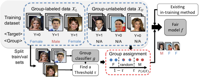
Figure 2: Overview of the proposed CGL strategy under the Fair-PG scenario. We train a fair model by assigning group pseudo-labels to group-unlabeled training set $\mathcal{X}_{U}$. We train an auxiliary group classifier $g$ to generate pseudo labels. Here, we assign random group labels to low confident samples as shown in the dotted red box of the figure ($A=0$ and $A=1$ indicates “Female” and “Male”, respectively). After assigning confidence-based pseudo-labels to the group-unlabeled training set, we apply a fair-training method to train a fair model $f$.

3 Problem Definition

In this section, we formally define our scenario, Fair-PG, and the fairness criterion, disparity of equality of opportunity (DEO), for the general $M$-ary classification problem.

3.1 Formal definition of Fair-PG

Let $X\in\mathcal{X}\subset\mathbb{R}^{d}$ be an input feature, $Y\in\mathcal{Y}=\{1,\dots,M\}$ be a target label. We also denote $A\in\mathcal{A}=\{1,\dots,N\}$ as a group label defined by one or multiple sensitive attributes. For example, if phenotype and gender are sensitive attributes, our group labels are $\{$lighter-skinned male, lighter-skinned female, darker-skinned male and darker-skinned female$\}$. Fair-PG assumes that the input space $\mathcal{X}$ is partitioned into the group-labeled and group-unlabeled sets, $\mathcal{X}_{L}$ and $\mathcal{X}_{U}$. That is, a sample $(x,a,y)\sim P(X,A,Y)$ has a group label if $x\in\mathcal{X}_{L}$, and vice versa if $x\in\mathcal{X}_{U}$ as illustrated in Fig. 2. With partially annotated group labels, our goal is to find a classifier $f:\mathcal{X}\rightarrow\mathcal{Y}$ not biased against the group label $A$ while predicting a target label that best corresponds to an input feature.

3.2 Fairness criterion

Various group fairness criteria have been proposed with different philosophies of how to define discrimination [22, 31, 15]. We consider the equal opportunity (EOpp) [31] for $M$-ary classification problem with non-binary group labels, while most of group fairness criteria assumes binary target or group labels. A classifier $f$ satisfies EOpp with respect to the sensitive group label $A$ and the target $Y$ if the model prediction $\tilde{Y}$ and $A$ are conditionally independent given $Y$, i.e., $\forall a,a^{\prime}\in\mathcal{A}$, $y\in\mathcal{Y}$, $P(\tilde{Y}=y|A=a,Y=y)=P(\tilde{Y}=y|A=a^{\prime},Y=y)$. For measuring the degree of unfairness of $f$ under the distribution $P(X|A,Y)$, we use two types of disparity of EOpp (DEO) upon taking the maximum or the average over $y$ as follows, respectively:

$$\Delta(f,P,y):= \Big{(}\max_{a,a^{\prime}}\Big{(}|\mathbb{E}_{P(X|A=a,Y=y)}[\mathbb{I}(f(X)=y)]$$

$$-\mathbb{E}_{P(X|A=a^{\prime},Y=y)}[\mathbb{I}(f(X)=y)]|\Big{)}\Big{)},$$ (1)

$$\Delta_{M}(f,P)\triangleq\max_{y}\Delta(f,P,y),\quad\Delta_{A}(f,P)\triangleq~{}\frac{1}{|\mathcal{Y}|}\sum_{y\in\mathcal{Y}}\Delta(f,P,y)$$ (2)

The above two metrics indicate the accuracy gap between groups given a target label and complement each other in showing the worst case and average accuracy gaps.

4 Confidence-based Group Label Assignment

In this section, we present our Confidence-based Group Label assignment (CGL), which is simple and readily applicable to any fair-training method for the Fair-PG scenario. Our method is described in details, and its theoretical understanding is provided as well.

4.1 Method overview

As the existing fair-training methods for group fairness explicitly utilize group labels to optimize the fairness constraints, they are not directly applicable to our Fair-PG problem. A naive approach to apply the existing methods to Fair-PG is to use only group-labeled samples for the training. Unfortunately, as we observed in Fig. 1 and our experiments, this naive baseline performs even worse than the scratch training method that only uses the target labels, in terms of fairness. As another baseline, we can employ a pseudo-labeling strategy [45] that assigns the estimated group labels to the group-unlabeled data by training a separate group classifier. The vanilla pseudo-labeling strategy enables the recent improvements in algorithmic fairness to be readily transferred into our Fair-PG scenario, other than the scratch training only with the labeled training set. However, since this vanilla pseudo-labeling strategy trains the group classifier only with the group-labeled training samples, the pseudo group labels can be noisy and incorrect. Compared to the SSL problem, the incorrect group pseudo labels may lead to a more severe issue in terms of fairness by propagating group label errors into the complex fair-training methods.

To that end, we employ Confidence-based Group Label assignment (CGL) to reduce the effects of incorrect pseudo-labels. As classifier confidences can be a proxy measure of the mis-classification for the given samples [30, 34], we assume that the low-confident predictions are incorrect. We assign random group labels to those less confident group prediction samples, drawn from the empirical conditional distribution of group labels $a$ given the target labels $y$ (i.e., $P(A|Y=y)$) (Line 4 in Algorithm 1). In Section 4.2, we make two theoretical contributions. One is to show that our strategy is better than the vanilla pseudo-labeling with respect to the DEO given metric in Section 2, and the other is to show that the random label assignment is equivalent to ignoring the fairness constraint for those random labeled, low-confident samples. In practice, we expect that our random labeling can play as a regularization method.

For our CGL, we need one hyperparameter, a confidence threshold $\tau$, to determine whether the given prediction is low confident. We split the given group-labeled training set into training and validation sets (Line 1 and 2 in Algorithm 1) and search the best confidence threshold $\tau$ satisfying the best accuracy on predicting whether the given prediction is correct or wrong (Line 3 in Algorithm 1). A similar threshold-based strategy is employed in the out-of-distribution sample detection task [34]. As shown in our experiment, there exists a sweet spot of the confidence threshold $\tau$, where $\tau=1$ is the same as the “random label” assignment to all group-unlabeled samples and $\tau=0$ is the same as the vanilla pseudo-labeling strategy. Once we have the group classifier and the confidence threshold, we assign the pseudo-group labels with our strategy and train the classifier with base off-the-shelf fair-training method on the pseudo-group labeled training samples. Algorithm 1 and Fig. 2 illustrate the overview of the proposed CGL.

Data: Group-labeled training set $\mathcal{X}_{L}$ and group-unlabeled training set $\mathcal{X}_{U}$.

Result: A set of pseudo group-labels $\tilde{A}$ for group-unlabeled training set $\mathcal{X}_{U}$.

1 Split $\mathcal{X}_{L}$ into training and validation sets $\mathcal{X}_{L}^{\text{tr}}$, $\mathcal{X}_{L}^{\text{val}}$.

2 Train a group classifier $g:\mathcal{X}\rightarrow S^{|\mathcal{A}|}$ using the training samples $(x,a,y)\sim\mathcal{X}_{L}^{\text{tr}}$, where $S^{|\mathcal{A}|}$ is ${|\mathcal{A}|}$-simplex.

3 Search a confidence threshold $\tau$ on $\mathcal{X}_{L}^{\text{val}}$ that satisfies $\max_{\tau}\sum_{x\in\{x|\max g(x)>\tau\}}\mathbb{I}(\arg\max g(x)=a)+\sum_{x\in\{x|\max g(x)\leq\tau\}}\mathbb{I}(\arg\max g(x)\neq a)$.

Assign group pseudo-labels $\tilde{a}$ to $(x,y)\sim\mathcal{X}_{U}$ by $\tilde{a}=\arg\max g(x)$ if $\max g(x)>\tau$, otherwise by sampling from the empirical conditional distribution of $a$ given $y$, i.e., $\tilde{a}\sim P(A|Y=y)$.

Algorithm 1 Confidence-based Group Label assignment (CGL)

4.2 Theoretical understanding of CGL

In this subsection, we provide theoretical understandings of why the random label assignment to low confident samples is better than the vanilla pseudo-label (PS) with respect to DEO ($\Delta$). We apply each strategy directly on the true group probability $P(A|X,Y)$, i.e., given an ideally trained group classifier. Our first theoretical result (Proposition 1) supports that the difference between DEO obtained by our CGL and the underlying DEO is smaller than the difference between the DEO obtained by the vanilla strategy and the underlying DEO. In other words, our PS with the random assignment is a better approximation of the true $P(A|X,Y)$ than the vanilla PS. The formal statement is as follows.

Proposition 1.

Assume a binary group $\mathcal{A}=\{0,1\}$. Let $\Delta(x,y;f,P)$ be the influence of $x$ on DEO, $\Delta(f,P)$ (abbreviated as $\Delta(x,y)$). That is, from $\Delta(f,P)=T(\sum_{x\in\{x|f(x)=1\}}|\Delta(x,y)|)$ where $T(\cdot)$ is the maximum or average over $y$, $\Delta(x,y)$ is defined as follows:

$$\Delta(x,y)\triangleq P(X=x|A=1,Y=y)-P(X=x|A=0,Y=y).$$

Let $\mkern 1.5mu\overline{\mkern-1.5muP\mkern-1.5mu}\mkern 1.5mu(A|X,Y)$ and $\widehat{P}(A|X,Y)$ be modified distributions by the vanilla pseudo labeling and CGL, respectively:

$$\mkern 1.5mu\overline{\mkern-1.5muP\mkern-1.5mu}\mkern 1.5mu(A=a|X=x,Y=y)=\mathbb{I}\left(P(A=a|X=x,Y=y)>0.5\right).$$

$$\widehat{P}(A=a|X=x,Y=y)$$

$$=\begin{cases}1,&\text{if }P(A=a|X=x,Y=y)\in[\tau,1].\\ P(A=a|Y=y)&\text{if }P(A=a|X=x,Y=y)\in(1-\tau,\tau).\\ 0,&\text{otherwise,}\end{cases}$$

where $0.5\leq\tau\leq 1$ is a threshold value. Then, we denote $\mkern 1.5mu\overline{\mkern-1.5muP\mkern-1.5mu}\mkern 1.5mu(X|A,Y)$ and $\widehat{P}(X|A,Y)$ as the distributions induced by $\mkern 1.5mu\overline{\mkern-1.5muP\mkern-1.5mu}\mkern 1.5mu(A|X,Y)$ and $\widehat{P}(A|X,Y)$. We also define $\mkern 1.5mu\overline{\mkern-1.5mu\Delta\mkern-1.5mu}\mkern 1.5mu(x,y)\triangleq{\Delta}(x,y;f,\mkern 1.5mu\overline{\mkern-1.5muP\mkern-1.5mu}\mkern 1.5mu)$ and $\widehat{\Delta}(x,y)\triangleq{\Delta}(x,y;f,\widehat{P})$ as the estimations of $\Delta(x,y)$ Then, for any classifier $f$, each $y$ and all $x\in\{x|f(x)=1\ \ \text{and}\ \ 1-\tau<P(A=1|X=x,Y=y)<\tau\}$, there exists a $\tau$ that satisfies following inequality:

$$|\Delta(x,y)-\mkern 1.5mu\overline{\mkern-1.5mu\Delta\mkern-1.5mu}\mkern 1.5mu(x,y)|>|\Delta(x,y)-\widehat{\Delta}(x,y)|.$$ (3)

The proof is in the Appendix. It helps to get a high-level understanding of the advantages of CGL over the vanilla PS although the Proposition 1 is not exactly equivalent to the inequality for $\Delta(f,P)$. In practice, due to the simplicity, we approximate the true distribution $P(A=a|X,Y)$ by one group classifier $g$ which learns $P(A=a|X)$, instead of training $|\mathcal{Y}|$ group classifiers for each $y$. As reported from our experiment in the Appendix, our group classifier approximates $P(A=a|X)$ well by achieving more than 85% group accuracy with 50% of group-labeled training data.

We also show that assigning random labels to a partition of the given data points, $\mathcal{X}_{U}$, is equivalent to ignoring the DEO constraint to the data points in $\mathcal{X}_{U}$:

Proposition 2.

Assume $\mathcal{X}$ is partitioned into any two sets, $\mathcal{X}_{L}$ and $\mathcal{X}_{U}$. Let $\widetilde{P}(A|X,Y)$ be a modified version of $P(A|X,Y)$ as follows:

$$\widetilde{P} (A=a|X=x,Y=y)$$

$$=\begin{cases}P(A=a|X=x,Y=y),&\text{if }x\in\mathcal{X}_{L}\text{.}\\ P(A=a|Y=y)&\text{otherwise.}\end{cases}$$

We denote $\widetilde{P}(X|A,Y)$ as a modified data distribution of $P(X|A,Y)$ induced by $\widetilde{P}(A|X,Y)$. Then, for any classifier $f$, $\Delta(f,P)$ is the same as $\Delta(f,\widetilde{P})$ using the partial set $\mathcal{X}_{L}$.

The proof is in the Appendix. In practice, since the existing fair-training methods use a relaxed version of DEO, our method can play as a regularization method to the group-unlabeled samples by assigning random group labels.

5 Experiments

In this section, we demonstrate the effectiveness of our CGL for the Fair-PG scenario. We evaluate CGL with various baseline fair-traning methods on three benchmark datasets: UTKFace [67] (the sensitive group is ethnicity), CelebA [46] (the sensitive group is gender) ProPublica COMPAS [36] (the sensitive group is ethnicity), and UCI Adult [21] (the sensitive group is gender) datasets, where COMPAS and Adult datasets are non-vision tabular datasets. We combine CGL with MFD [37], FairHSIC [51] and Re-weighting [35]. To understand the trained group classifier, we provide extensive analysis on the group classifier. Finally, we show the strong empirical contribution of CGL by utilizing extra group-unlabeled training data on the UTKFace dataset. Our CGL shows significant improvements on the target accuracy and the group fairness compared to the baseline methods.

5.1 Experimental settings

5.1.1 Datasets

UTKFace[67]. UTKFace is a facial image dataset, widely adopted as a multi-class and multi-group benchmark. UTKFace contains more than 20K images with annotations, such as age (range from 0 to 116), gender (male and female) and ethnicity (“White”, “Black”, “Asian”, “Indian” and “Others”). We set ethnicity and age as the sensitive attribute and the target label, respectively. We divided the target age range into three classes: ages between 0 to 19, 20 to 40 and more than 40, following Jung et al. [37]. We use four ethnic groups, “White”, “Black”, “Asian” and “Indian”, while “Others” is excluded. The test set is constructed to contain the same number of samples for each group and target.

CelebA[46]. CelebA contains about 200K face images annotated with 40 binary attributes. As the previous works [37] and [53], we picked up “Blond Hair” and “Attractive” as the target labels and “Gender”(denoted as “Male” in the dataset) as the sensitive attribute. The results for “Attractive” and ethical concerns are provided in the Appendix. The test set is constructed as the same as UTKFace.

ProPublica COMPAS[36]. We also consider a non-vision tabular dataset to show the versatility of CGL to other modalities. We use the ProPublica COMPAS dataset, a binary classification task where the target label is whether a defendant reoffends. We set ethnicity as the sensitive attribute and used the same pre-processing as Bellamy et al. [6], thereby it includes 5,000 data samples, binary group (“Caucasian” and “Non-Caucasian” and target labels.

In addition, we also give details and results on UCI Adult[21] dataset in the Appendix.

5.1.2 Base fair-training methods

We employ three state-of-the-art in-processing methods, MMD-based Fair Distillation (MFD) [37], FairHSIC [51] and Label Bias Correction (LBC) [35] for the base fair-training method of CGL. We briefly describe each method in the Appendix. We only consider scalable fair-training methods for deep learning-based vision applications; note the primal approaches in group fairness [39, 63] cannot be applied to the vision domain with high dimensional data and complex models (e.g., DNNs). We emphasize, however, that our method is not confined to the three methods used in this study but can be easily applied to any fair-training method.

5.1.3 Implementation details

We provide the implementation details in the Appendix, including the details of architectures and optimizers, the hyperparameter search protocol.

Model selection.

For fairness-aware learning on real datasets, there can exist a trade-off between accuracy and fairness (see an example of the trade-off in Fig. 6). For fair comparison, we should select the optimal hyperparmeters showing the best for one criterion while maintaining similar performance for others. Therefore, we select the hyperparameter showing the best fairness criterion $\Delta_{M}$ while achieving at least 95% of the vanilla training model accuracy for UTKFace and CelebA datasets. We set the lower bound to 90% for the COMPAS dataset. If there exists no hyperparameter achieving the minimum target accuracy, we report the hyperparameter with the best accuracy. All models are chosen from the last training epoch.

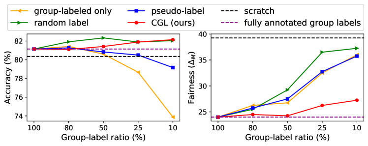
(a) MFD results

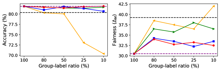
(b) FairHSIC results

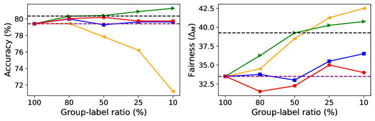
(c) LBC results

Figure 3: Results on UTKFace. For varying group-label ratios in training dataset, we show the combination of three fair-training methods with “group-labeled only” (yellow), “random label” (green), “pseudo-label” (blue) and our CGL (red). “scratch” denotes the vanilla training without a fairness criteria and “fully annotated group labels” denotes the fair-training methods using the full group labels (i.e., when group-label ratio is 100%). Higher accuracy and lower $\Delta_{M}$ denote improvements, respectively.

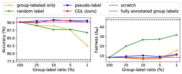
(a) MFD results

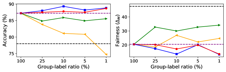
(b) FairHSIC results

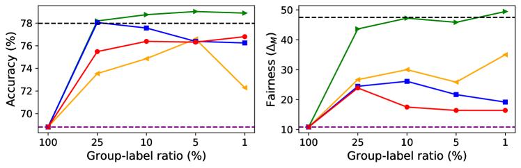
(c) LBC results

Figure 4: Results on CelebA. The details are the same as Fig. 3.

Baseline methods and evaluation metrics.

The existing in-processing methods for group fairness are not applicable directly to our scenario, i.e., when the group labels are not fully annotated. Also, as mentioned in Sec. 2, the existing SSL methods mostly cannot be directly applied to Fair-PG as well, since it is not clear whether they achieve the group fairness when applied to predict non-annotated group labels (see the results of UPS [52] in the Appendix, which is one of the state-of-the-art SSL methods). We hence employ three straightforward baselines for comparison. The group-labeled only strategy discards the group-unlabeled samples and only uses the group-labeled samples for the training. We also examine two group label assignment strategies: The random label strategy assigns random labels to all of the group-unlabeled data (drawn from $P(A|Y=y)$), while the pseudo-label strategy fully trusts the group classifier predictions. Each method is an extreme case of CGL by setting $\tau=1$ and $\tau=0$, respectively. We note that based on the Proposition 2, “random label” has the same effect on evaluating the fairness loss part only with the group-labeled samples while evaluating the main loss with all the samples.

We considered three evaluation metrics for all experiments, the target accuracy, $\Delta_{M}$ and $\Delta_{A}$ (see Eq. 2). The results are the average scores of four different runs on UTKFace and COMPAS and two different runs on CelebA. $\Delta_{A}$ and standard deviation scores are given in the Appendix.

5.2 Main results

Fig. 3 compares the target accuracies and $\Delta_{M}$ of the combination of MFD, FH and LBC with three baseline strategies and CGL on the UTKFace dataset with different group-label ratios from 100% (fully group annotated) to 10 %. We show the similar results on the CelebA dataset in Fig. 4 where group-label ratio is chosen from 100% to 1%. Note that we choose different group-label ratios to the datasets because UTKFace is multi-class and multi-group dataset, and CelebA is binary-class and binary-group dataset. We also emphasize that the performance comparison of the three baselines and CGL mainly focus on $\Delta_{M}$ because we reported the best $\Delta_{M}$ of each method among models having accuracy more than the accuracy lower bound described in Sec. 5.1.3.

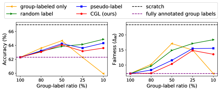
(a) MFD results

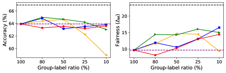
(b) FairHSIC results

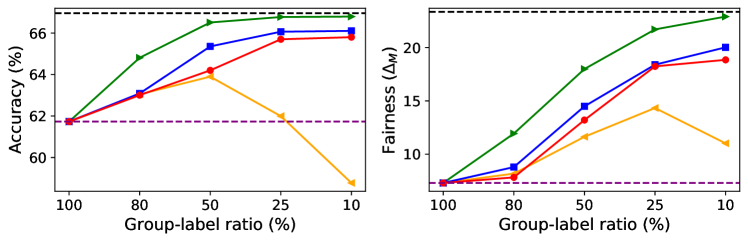
(c) LBC results

Figure 5: Results on COMPAS. The details are the same as Fig. 3.

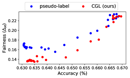
Figure 6: Accuracy-fairness trade-off on COMPAS with 10% group-labeled training set. We show accuracy and $\Delta_{M}$, obtained for CGL and “pseudo label” combined with MFD, for different hyperparameters of MFD..

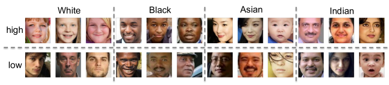
Figure 7: High and low confident samples by the group classifier on UTKFace.We illustrate the top-3 highest and lowest confident samples for that the classifier predicts the correct answer from the UTKFace training samples for each group.

In the figures, the “group-labeled only” (yellow line) consistently shows much worse accuracies than the baseline methods. Especially, when the group-label ratio decreases, “group-labeled only” drastically harms accuracy and fairness at the same time. The “random label” (green line) strategy rarely hurts the accuracies since it uses the full target labels for training, but it shows a drastic drop in $\Delta_{M}$. The “pseudo-label” (blue line) performs better than the other baselines, but the classifier errors severely affect the fairness performances, especially in the multi-group scenario (e.g., UTKFace). On the other hand, CGL shows consistently better performances than other baselines in most cases, most notably on UTKFace, by successfully handling samples with low confident group predictions.

We also report the results on non-vision tabular dataset in Fig. 5. We observe similar results to Fig. 3 and Fig. 4. Note that “group-labeled only” shows better fairness criterion in price of the rapid decrease of accuracy in the low group label regime. Our method generally performs better than other baselines in all methods in terms of fairness. We point out that although the accuracies of CGL are slightly lower than those of the other baselines, it does not necessarily mean that those schemes perform better since they must sacrifice much more accuracy to achieve similar $\Delta_{M}$ to CGL. To clarify this, we plotted the full accuracy-fairness trade-offs with different hyperparameters on COMPAS in Fig. 6. We clearly observe that CGL dominates “pseudo label” by achieving a better Pareto trade-off curve, which implies the validity of our model selection rule given in Section 5.1.3.

5.3 Analysis of group classifiers

Group classifier confidences.

We show the highest and lowest confident samples by the group classifier on UTKFace in Fig. 7. As shown in the figure, the low confident samples are qualitatively uncertain to humans due to diverse lighting, various orientations and low quality. Therefore, our confidence-based thresholding can capture the inherent uncertainty of the dataset. In the Appendix, we provide the confidence score distribution and the group classifier accuracies for different group label ratios.

Study on the threshold $\tau$.

Figure 8 shows the accuracies and $\Delta_{M}$ of CGL and MFD by varying $\tau$ on UTKFace with 10% group-labeled training set. We fix the hyperparameters used in Fig. 3 and report the average of two different runs. $\tau\leq 0.25$ (since there are four groups) and $\tau=1$ is equivalent to “random label” and “pseudo-label” in the previous results, respectively. The “$\star$” represents the results of $\tau$ achieved by the our strategy (Line 4 in Algorithm 1). Here, we observe that there exists a sweet spot of the threshold that shows better $\Delta_{M}$ and accuracy than “random label” and “pseudo-label”, and our method can achieve a good threshold near the sweet spot.

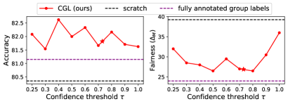
Figure 8: $\tau$ study on UTKFace. Accuracies and fairness (by $\Delta_{M}$) for varying $\tau$. $\tau\leq 0.25$ is the same as “random label” and $\tau=1$ corresponds to vanilla “pseudo-label” in other figures.

5.4 Augmenting with extra group-unlabeled data

We finally show the impact of the Fair-PG scenario and our CGL on the UTKFace dataset and an extra group-unlabeled dataset. We use the FairFace dataset [40] for the extra dataset. FairFace contains 108,501 facial images with balanced attributes. We filter out ethnicity not in “White”, “Black”, “Asian” and “Indian”. After the filtering, we have 73,377 extra samples. To examine our Fair-PG problem, we let the extra datasets only have the target labels (i.e., ages) but not the group labels. Tab. 1 shows the results of the scratch and MFD trained only on the UTKFace, and the scratch and MFD+CGL on the UTKFace augmented with the FairFace dataset as above. Interestingly, MFD on UTKFace only shows worse fairness ($\Delta_{M}=25.0$) than the scratch training on the UTKFace + FairFace ($\Delta_{M}=24.0$), which is in line with the result on low group label regime in (Fig. 1). We achieve the state-of-the-art accuracy (84.38%) and fairness ($\Delta_{M}=19.5$) by successfully augmenting UTKFace with the extra group-unlabeled dataset.

Table 1: Impact of CGL on UTKFace and extra group-unlabeled training dataset. The accuracy and fairness criterion on the UTKFace test set are shown. For “MFD + CGL”, we assign group psuedo-labels by CGL to the extra group-unlabeled samples from FairFace (73,377 images) with the group classidier trained on full UTKFace training set (20,813 images). We then train MFD on the psuedo-labeled training dataset (94,190 images).

	UTKFace only		UTKFace + FairFace
	Scratch	MFD	Scratch	MFD + CGL
Accuracy ($\uparrow$)	80.29	83.46	81.15	84.38
Fairness $\Delta_{A}$ ($\downarrow$)	20.17	16.67	15.67	13.00
Fairness $\Delta_{M}$ ($\downarrow$)	39.00	25.00	24.00	19.50

6 Concluding Remark

We considered a practical learning scenario in which the group labels are partially annotated for fariness-aware learning. We have observed that the existing fair-training method can even perform worse than the scratch training when the number of group labels is small. We propose a simple yet effective solution that is readily applicable to any fair-training method and demonstrated that CGL improves various baselines on several benchmarks. We believe our method can significantly reduce the cost for obtaining additional group labels for all the training samples, facilitating more rapid development of fair classifiers.

Supplementary Materials

We include additional materials in this document. We first state our societal impact, dataset license, limitations and ethical concerns in the beginning. We provide additional related works for biases in machine learning in Appendix B and a detailed proof of our propositions in Appendix A. We include our implementation details, such as architecture, optimization, hyperparameter search and base fairness methods and their modifications in Appendix C. We provide the additional analysis of group classifiers in Appendix D, experimental results in Appendix E and result tables in Sec. E.5.

Dataset license.

In the paper, we use four datasets: UTKFace [67], CelebA [46], ProPublica COMPAS [36] and FairFace [40]. According to the official web page, UTKFace dataset is a non-commercial license dataset where the copyright belongs to the original owners in the web. The dataset is built by Dlib [42] and annotations are tagged by the DEX algorithm and human annotators. CelebA dataset has a similar license statement to UTKFace. COMPAS dataset is collected its data points from Broward County Sheriff’s Office in Florida which is a public records. FairFace is licensed by CC by 4.0. Overall, all datasets have clean licenses that is applicable to any public research project.

Societal impact.

As we stated in the main text, a vanilla DNN training can occur negative societal impacts by dismissing fairness criterion, on the other hand, considering fairness criterion at the training time requires a huge number of group labels. We expect our CGL can bridge the gap between real-world applications and fairness-aware training, so that mitigating the negative societal impacts economically by only annotating a subset of group-unlabeled samples.

Limitations.

Although our method can be applied to any fairness method, we observe that CGL is not always better than other baselines. First, our method relies on the quality of group classifier, hence, if the group classifier performs worse, our method does not guarantee better fairness than the vanilla pseudo-labeling. Also, the group classifier predictions can be noisy. In Appendix, we show group prediction accuracy of our group classifier. In the low group label regime, the accuracy of our classifier decreases to less than 80% on UTKFace. This implies that if the base method is sensitive to noisy group labels (e.g., Adversairal De-biasing), our method and pseudo-labeling can perform worse than our expectation. Finally, in the case that a distribution shift for the sensitive attribute exists when predicting group labels of group-unlabeled data from group-unlabeled data, the naive application of would suffer from performance degradation. These distribution shift can be alleviated by training a group classifier with robust optimization techniques (e.g., choosing a distribution shift-aware optimizer [12], invariant risk minimization [4] or group distributed robust optimization [53]).

Ethical concerns

We originally used a subjective and potentially unethical “Attractive” attribute in our experiments with the CelebA dataset. It is known that “Attractive” is highly correlated to gender (“Male”), while most other attributes are not [58]. Our purpose of CelebA experiments is to show the scalability of our method as CelebA (200K) is a large-scale dataset compared to UTK (20K), COMPAS (5K), Adult (40K). From a similar motivation, many previous studies employed Attractive as their target label [37, 16, 50, 51]. Particularly, Quadrianto et al. used Attractive “as the proxy measure of getting invited for a job interview in the world of fame” [51]. However, we agree that using a subjective attribute as “Attractive” can be unethical. We only used the results as an example, and we alert that such classifiers for attractiveness can cause potential ethical concerns.

Appendix A Proof of propositions

A.1 Proof of Proposition 1

Proof.

We only show only the case where $P(A=1|X=x,Y=y)\geq 0.5$ and the opposite case can be proved in the same way. For any classifier $f$ and all $x\in\{x|f(x)=1\,\text{and }0.5\leq P(A=1|X=x,Y=y)<\tau\}$, we have from $\mkern 1.5mu\overline{\mkern-1.5muP\mkern-1.5mu}\mkern 1.5mu$ and $\widehat{P}$ defined in (Eq. (3) and (4), manuscript),

$$\mkern 1.5mu\overline{\mkern-1.5mu\Delta\mkern-1.5mu}\mkern 1.5mu(x,y) =\big{(}\frac{1}{P(A=1|Y=y)}\big{)}P(X=x|Y=y),$$ (A.1)

$$\widehat{\Delta}(x,y) =0.$$ (A.2)

Then, we have

$$|\Delta(x,y)-\mkern 1.5mu\overline{\mkern-1.5mu\Delta\mkern-1.5mu}\mkern 1.5mu(x,y)|-|\Delta(x,y)-\widehat{\Delta}(x,y)|=\begin{cases}\mkern 1.5mu\overline{\mkern-1.5mu\Delta\mkern-1.5mu}\mkern 1.5mu(x,y)\quad&\text{if }\Delta(x,y)\leq 0\\ \mkern 1.5mu\overline{\mkern-1.5mu\Delta\mkern-1.5mu}\mkern 1.5mu(x,y)-2\Delta(x,y)\quad&\text{otherwise.}\end{cases}$$ (A.3)

For the first case in Eq. A.3, we can trivially see that $\Delta(x,y)>0$. For the second case in Eq. A.3, we have

$$\mkern 1.5mu\overline{\mkern-1.5mu\Delta\mkern-1.5mu}\mkern 1.5mu(x,y)-2\Delta(x,y)$$ (A.4)

$$=\big{(}\frac{1-2P(A=1|X=x,Y=y)}{P(A=1|Y=y)}+\frac{2P(A=0|X=x,Y=y)}{P(A=0|Y=y)}\big{)}P(X=x|Y=y)>0$$ (A.5)

, if $P(A=1|X=x,Y=y)<\frac{P(A=1|Y=y)+1}{2}$. Therefore, we have the proposition 1 by setting $\tau$ to $\frac{P(A=1|Y=y)+1}{2}$. ∎

A.2 Proof of Proposition 2

Proof.

Given a data distribution $P(X,A,Y)$ and a classifier $f$, $\Delta(f,P)$ is defined as follows:

$$\Delta(f,P)=T\bigg{(}\max_{a,a^{\prime}}\big{(}|\underbrace{P(\hat{Y}=y|A=a,Y=y)-P(\hat{Y}=y|A=a^{\prime},Y=y)}_{(a)}|\big{)}\bigg{)}$$ (A.6)

, where $T(\cdot)$ can be the maximum or average over $y$ depending on the types of $\Delta$. For each $y,a$ and $a^{\prime}$, the above argument of $\max_{a,a^{\prime}}$, (a) in Eq. A.6, can be represented as follows:

$$(a) =\sum_{x\in\{x|f(x)=y\}}P(X=x|A=a,Y=y)-P(X=x|A=a^{\prime},Y=y)$$

$$=\sum_{x\in\{x\in X_{L}|f(x)=y\}}P(X=x|A=a,Y=y)-P(X=x|A=a^{\prime},Y=y)$$

$$\quad+\sum_{x\in\{x\in X_{U}|f(x)=1\}}P(X=x|A=a,Y=y)-P(X=x|A=a^{\prime},Y=y)$$ (A.7)

Then, the second term of Eq. A.7 can be represented as follows:

$$\sum_{x\in\{x\in X_{U}|f(x)=y\}}P(X=x|A=a,Y=y)-P(X=x|A=a^{\prime},Y=y)$$

$$=\sum_{x\in\{x\in X_{U}|f(x)=y\}}\frac{P(A=a|X=x,Y=y)P(X=x|Y=y)}{P(A=a|Y=y)}-\frac{P(A=a^{\prime}|X=x,Y=y)P(X=x|Y=y)}{P(A=a^{\prime}|Y=y)}$$ (A.8)

If we substitute $P(A|X,Y)$ into $\widehat{P}(A|X,Y)$ in the RHS of Eq. A.8, we have the proposition 2. ∎

Appendix B Additional Related Works for Biases in Machine Learning

Emerging studies on DNNs have revealed that DNNs rely on shortcut biases [11, 27, 5, 26, 54]. The existing de-biasing methods let a model less attend on the dataset biases in an implicit way by using extra biased networks [11, 5] or data augmentations [27] without using bias labels. Both fairness methods and de-biasing methods aim to learn a representation invariant to undesired decision cues, such as sensitive groups and dataset biases. However, de-biasing methods explore implicit shortcut biases that harm the network generalizability, where many known shortcuts (e.g., language bias [11] or texture bias [27]) are neither strongly relative to ethical concerns nor easy to configure. On the other hand, in the fairness problem, sensitive groups are diversely defined by the target application to avoid negative societal impacts (i.e., a model should make the same predictions to any social group such as ethnicity or gender). Therefore, even though de-biasing methods can be applied to Fair-PG by ignoring group labels, there is no guarantee to learn fair models by the de-biasing approaches. In this work, we focus on fairness methods explicitly utilizing group labels for the base method of CGL.

Appendix C More Implementation Details

C.1 Architecture and optimization

We choose the same architecture for the base classifier and the group classifier; ResNet18 [33] for the UTKFace and CelebA experiments and a simple 2-layered neural network for the COMPAS experiments. On UKTFace and CelebA datasets, we train the models with the Adam optimizer [43] for 70 epochs by setting the initial learning rate 0.001 reduced by 0.1 when the loss is stagnated for 10 epochs following Jung et al. [37]. We train the model for 50 epochs on COMPAS dataset. All results are reported by the model at the last epoch.

C.2 Hyperparameter search

In the experiments, there are two types of hyperparameters: the confidence threshold of CGL, and the method-specific hyperparameters for each method. Since our method only needs the group-labeled training dataset for training group classifier and seeking a threshold, we split the group-labeled samples into 80% training and 20% validation samples. The confidence threshold is searched on the validation set (by Algorithm 1, manuscript).

Fairness-aware training methods are usually sensitive to the hyperparameter selection due to the accuracy-fairness trade-off; when the strength for fairness is getting stronger, the target accuracy is getting worse. For example, a trivial solution to achieve the fairest classifier is to predict all labels to a constant label, while this solution is the worst solution in terms of the target accuracy. Hence, the careful tuning of the control parameters to fairness criteria (e.g., MMD [37], HSIC [51] or adversarial loss [65]) takes the key role in handling the accuracy-fairness trade-off. In our experiments, we aim to find a fair classifier while showing a comparable accuracy to the vanilla training method. Thus, we select the hyperparameter showing the best fairness criterion $\Delta_{M}$ while achieving at least 95% of the vanilla training model accuracy. We set the lower bound to 90% for the COPMAS dataset. If there exists no hyperparameter achieving the minimum target accuracy, we report the hyperparameter with the best accuracy. We perform the grid search on the hyperparameter candidates for every partial group-label case and for every method. The full hyperparameter search space is illustrated in Tab. C.1.

Method	Hyperparameter	Candidates
MFD [37]	MMD strength $\lambda$	[10, 30, 100, 300, 1000, 3000, 10000, 30000]
FairHSIC [51]	HSIC strength $\lambda$	[1,3,10, 30, 100, 300, 1000, 3000]
LBC [35]	Adversary strength $\alpha$	[1, 3, 10, 30, 100]
	learning rate of adversary	[$10^{-4}$, $10^{-2}$]

Table C.1: Hyperparameter search spaces. We perform the grid search on the validation set to find the best hyperparameters for each method. We use the same hyperparameters for optimizer (See Sec. C.1).

C.3 Base fairness methods and their modifications

Here, we describe the overview of each base fairness method used for the experiments. MFD and FairHSIC use additional fairness-aware regularization terms as the relaxed version of the targeted fairness criteria. MFD proposed a maximum-mean-discrepancy-based [28] regularization term to achieve fairness via feature distillation and FairHSIC devised a HSIC-based [29] regularization term to obtain feature representations independent on group labels. For FairHSIC, we only implement the second term of their decomposition loss (i.e., the HSIC loss between the feature representations and the group labels).

LBC is a re-weighting algorithm optimizing weights of examples through multiple iterations of full training to ensure their theoretical guarantees. The original LBD requires multiple full-training iterations by alternatively computing a EO criterion after full-training and re-training the full dataset by optimal weights. This alternative optimization needs a very huge training budget. We modify the EO computation iteration to a few-epoch iterations, i.e., 5 epochs, instead of the full-training.

AD lets an adversary cannot predict group labels by the additional adversarial loss. In our experiments, AD shows little improvements if the group or target label is not binary where Jung et al. [37] witnessed the same phenomenon. Thus, we use multiple adversaries for AD to make AD be available to solve multi-class and multi-group problems following Jung et al. [37] and omit the loss projection in the original objectives of AD for a stable learning. Also, we only report AD results for the Compas dataset while AD does not perform well on other vision datasets.

Appendix D Additional Analysis of Group Classifiers

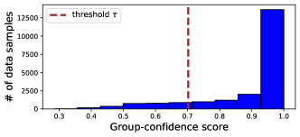
Figure D.1: Group confidences verse sample densities. The number of samples for each confidence bin is shown. The red dotted line denotes the selected threshold in the UTKFace experiments.

Table D.1: Group classifier performances. We compare the accuracies by the baseline decision rule ($\arg\max$) and by our method (assigning random labels to low confident samples) for the trained group classifiers on the small group-labeled training samples.

Group-label ratio	80%	50%	25%	10%
Baseline	87.88	86.11	82.82	77.73
Ours	87.24	85.81	82.59	75.21

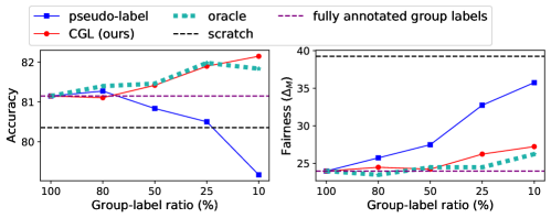
Figure D.2: Comparisons with an “oracle” fair group classifier on UTKFace with MFD. The oracle classifier group classifier has the same accuracy with our group classifier (used for “pseudo-label” and “CGL (ours)” – See Tab. D.1) but the wrong samples by the “oracle” classifier are randomly chosen from the dataset.

Prediction confidences by our group classifier.

In the main manuscript, we show the highest and lowest confident samples by the group classifier on UTKFace in Fig. 7. As shown in the figure, low confident samples are qualitatively uncertain to humans due to diverse lighting, various orientations and low quality, where Shi et al. observed the same results by an uncertainty-aware face embedding [55]. From the qualitative results, we observe that our confidence-based threshold method can reasonably capture the inherent uncertainty of the dataset without an explicit uncertainty-aware training, such as MC-Dropout [24] or probabilistic embeddings [49, 18].

However, because our group classifier does not guarantee to capture proper uncertainty measures, we presume that applying an uncertainty-aware training can improve CGL as Rizve et al. [52]. We show the number of samples by the confidences in Fig. D.1. Our classifier shows high confident predictions (over 65% predictions are confident than 0.9 because) because it is not trained by calibration-aware regularizations [30] or other regularization techniques known to help confidence calibration scores [19], such as mixed sample augmentations [66, 61] and smoothed labels [57]. Nonetheless, we observe that many images are still low confident and our group classifier can figure whether the prediction is correct or wrong; when we apply the optimal threshold, our classifier has 85.43% accuracy to figure out whether the prediction is wrong or correct.

Quality of our group classifier and the threshold-based decision rule.

In Tab. D.1, we show the group accuracies of our group classifier by different decision rules on varying group label ratio. We show two different decision rules: the baseline $\arg\max$ strategy and our confidence-based random altering (i.e., $\arg\max$ if the confidence is larger than $\tau$, otherwise $P(A|Y)$) with the best threshold. We observe that our random label strategy slightly hurts the accuracies but not significantly. In other words, our group classifier has well-sorted confidences that can capture the self predictive uncertainty.

Finally, we compare our group classifier and the “oracle” group classifier which has the same accuracy to ours, but group labels that our group classifier wrongly predict are replaced into a group label sampled from an uniform distribution. In other words, “oracle” assumes the scenario where our confidence-based thresholding perfectly operates. Fig. D.2 shows the comparison of CGL, “pseudo-label” and “oracle” on UTKFace dataset and MFD. Here, we see that “oracle” significantly improve the performance in terms of fairness other than “pseudo-label”. This imply that only random-labeling for wrongly predicted group labels can prevent performance degradation of DEO, which experimentally supports our proposition 2. We also observe that the performance of CGL is comparable one of “oracle”, meaning that random labeling low confident samples are more critical to the performance than high confident samples with noisy group labels.

Appendix E Additional experimental results

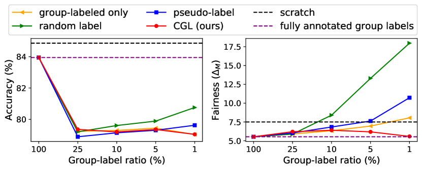
(a) MFD results on Adult

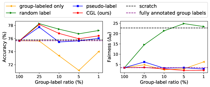
(b) MFD results on CelebA

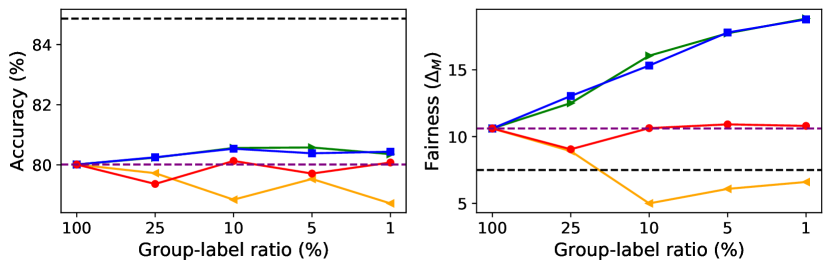
(c) FairHSIC results on Adult

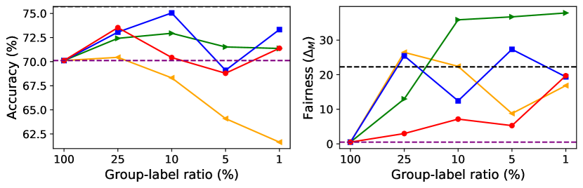
(d) FairHSIC results on CelebA

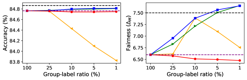
(e) LBC results on Adult

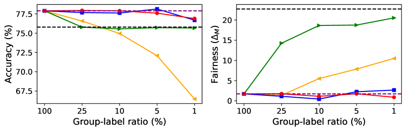
(f) LBC results on CelebA

Figure E.1: Results on Adult and CelebA. The target label in CelebA is “Attractive” attribute. The details are the same as Fig. 3.

E.1 Results on Adult dataset

To show the consistent improvements on another dataset, we conducted an additional experiment on Adult dataset with the same details as the main experiment in the manuscript. UCI Adult dataset [21] is a non-vision tabular dataset used for a binary classification task where the target label is whether the income exceeds $50K per a year given attributes about the person. We set gender as the sensitive attribute and used the same processing as Bellamy et al. [6], so that it includes 45,000 data samples.

The left column of Fig. E.1 shows the results of CGL and baselines combined with base fairness methods on Adult dataset, and we observe the consistent trend of CGL that our method mostly performs better than other baselines for fairness. We repeatedly note that our slightly lower accuracies do not imply the ineffectiveness of CGL because we report the model with the best DEO where accuracy is lower-bounded.

E.2 Results on CelebA using the “Attractive” attribute as the target label

The right column of Fig. E.1 shows the target accuracy and $\Delta_{M}$ on CelebA using “Attractive” attribute as the target label. From the right column of Fig. E.1, we again demonstrate the better performance of CGL than other baselines for all base fairness methods. Since the “Attractive” attribute would be the subjective and potentially unethical to discuss the results rigorously, as described in the beginning of Appendix, we advise that these results should used only as a auxiliary and not as a primary result.

E.3 Comparison CGL with UPS

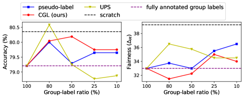
Figure E.2: LBC results on UTKFace

The aim for SSL is to simply predict the future attribute labels as accurately as possible from the partial annotations in the training set, it is not clear whether the predicted attribute labels can be directly plugged-in to achieve the group fairness in the test set. To corroborate our finding, we carried out additional experiments with a state-of-the-art SSL method, UPS, utilized for Fair-PG. UPS iteratively trains the group classifier and predicts the missing group labels in the training set and filters out the samples with uncertain predictions. (We omitted the negative learning of UPS since it cannot be applied any base fairness methods.) Note such filtering would unnecessarily discard significant amount of the target label information, hence, the accuracy would hurt particularly when the group label ratio is low. In Fig. E.2, we report the result of LBC on UTKFace, including the UPS baseline. We indeed observe that UPS suffers from low accuracy especially when the group-label ratio is low, and CGL mostly outperforms UPS for both accuracy and fairness. This confirms that a naive plug-in of SSL method for Fair-PG would not be satisfactory.

E.4 AD results on COMPAS dataset

Table E.1: Accuracy on COPMAS for AD.

	100%	80%	50%	25%	10%
group-labeled only	63.51 ($\pm$1.45)	65.32 ($\pm$0.58)	63.65 ($\pm$0.37)	61.30 ($\pm$1.22)	57.52 ($\pm$2.84)
random label		63.61 ($\pm$0.55)	63.11 ($\pm$0.67)	64.44 ($\pm$1.38)	64.67 ($\pm$0.24)
psuedo-label		64.55 ($\pm$0.41)	64.12 ($\pm$0.63)	63.19 ($\pm$0.18)	65.80 ($\pm$0.38)
CGL		63.05 ($\pm$1.13)	63.25 ($\pm$0.60)	64.24 ($\pm$1.24)	63.82 ($\pm$1.55)

Table E.2: $\Delta_{A}$ on COPMAS for AD.

	100%	80%	50%	25%	10%
group-labeled only	10.35 ($\pm$1.84)	13.32 ($\pm$2.14)	11.46 ($\pm$0.63)	9.75 ($\pm$1.84)	5.27 ($\pm$0.76)
random label		9.26 ($\pm$1.46)	10.69 ($\pm$1.46)	13.17 ($\pm$2.10)	11.90 ($\pm$1.44)
psuedo-label		12.43 ($\pm$3.39)	12.11 ($\pm$4.07)	11.37 ($\pm$3.17)	16.26 ($\pm$0.57)
CGL		9.63 ($\pm$3.60)	11.93 ($\pm$3.90)	14.71 ($\pm$1.27)	10.67 ($\pm$2.70)

Table E.3: $\Delta_{M}$ on COPMAS for AD.

	100%	80%	50%	25%	10%
group-labeled only	12.72 ($\pm$2.98)	16.30 ($\pm$2.41)	14.39 ($\pm$1.50)	12.61 ($\pm$2.11)	8.52 ($\pm$2.22)
random label		12.37 ($\pm$2.09)	13.51 ($\pm$1.38)	15.96 ($\pm$1.93)	15.70 ($\pm$2.26)
psuedo-label		16.15 ($\pm$3.79)	15.68 ($\pm$4.73)	13.97 ($\pm$2.67)	19.57 ($\pm$0.93)
CGL		13.78 ($\pm$5.00)	14.73 ($\pm$5.28)	17.96 ($\pm$0.31)	13.23 ($\pm$3.82)

Tab. E.1, Tab. E.2 and Tab. E.3 compare the target accuraies, $\Delta_{A}$ and $\Delta_{M}$ of the combinations of AD with three baselines and CGL on COMPAS dataset. The number in the parentheses with $\pm$ stands for the standard deviation of each metric obtained several independent runs with different seeds. our CGL again show the better performances than other baselines in terms of fairness for most cases. Through the case where the group-label ratio is 25%, we can see that confidence-based thresholding by a group classifier can be slightly sensitive in the group label regime if the base fairness method is vulnerable to noisy group labels (e.g., AD).

E.5 Result tables

Table from E.4 to E.30 show the detailed results including accuracy, $\Delta_{A}$ and $\Delta_{M}$ for all experiments in Figure 3, 4 and 5 in the main manuscript. The details of numbers in parentheses are the same as tables in Sec. E.4.

Table E.4: Accuracy on UTKFace for MFD.

	100%	80%	50%	25%	10%
group-labeled only	81.15 ($\pm$0.28)	81.42 ($\pm$0.39)	80.60 ($\pm$0.37)	78.67 ($\pm$0.64)	73.88 ($\pm$0.78)
random label		81.92 ($\pm$0.36)	82.33 ($\pm$0.53)	81.90 ($\pm$0.63)	82.04 ($\pm$0.34)
psuedo-label		81.27 ($\pm$0.60)	80.83 ($\pm$0.39)	80.50 ($\pm$0.54)	79.17 ($\pm$0.54)
CGL		81.10 ($\pm$0.24)	81.42 ($\pm$0.42)	81.90 ($\pm$0.41)	82.15 ($\pm$0.58)

Table E.5: $\Delta_{A}$ on UTKFace for MFD.

	100%	80%	50%	25%	10%
group-labeled only	15.67 ($\pm$0.71)	16.33 ($\pm$0.85)	17.08 ($\pm$1.46)	18.50 ($\pm$1.38)	21.25 ($\pm$2.66)
random label		16.83 ($\pm$0.29)	18.58 ($\pm$0.83)	22.58 ($\pm$0.86)	23.50 ($\pm$1.80)
psuedo-label		16.33 ($\pm$0.97)	16.67 ($\pm$0.41)	18.58 ($\pm$1.95)	20.00 ($\pm$2.16)
CGL		15.33 ($\pm$1.03)	14.92 ($\pm$2.17)	17.17 ($\pm$1.57)	17.25 ($\pm$1.04)

Table E.6: $\Delta_{M}$ on UTKFace for MFD.

	100%	80%	50%	25%	10%
group-labeled only	24.00 ($\pm$1.58)	26.25 ($\pm$3.56)	26.75 ($\pm$2.59)	32.50 ($\pm$2.87)	36.00 ($\pm$2.92)
random label		25.50 ($\pm$1.66)	29.25 ($\pm$4.66)	36.50 ($\pm$0.50)	37.25 ($\pm$3.19)
psuedo-label		25.75 ($\pm$2.86)	27.50 ($\pm$0.87)	32.75 ($\pm$3.83)	35.75 ($\pm$4.49)
CGL		24.50 ($\pm$2.06)	24.25 ($\pm$2.17)	26.25 ($\pm$3.49)	27.25 ($\pm$2.77)

Table E.7: Accuracy on UTKFace for FairHSIC.

	100%	80%	50%	25%	10%
group-labeled only	81.85 ($\pm$0.23)	80.29 ($\pm$0.64)	80.02 ($\pm$1.10)	73.04 ($\pm$3.68)	70.38 ($\pm$1.27)
random label		81.67 ($\pm$0.48)	81.44 ($\pm$0.78)	81.40 ($\pm$0.78)	81.65 ($\pm$0.56)
psuedo-label		81.00 ($\pm$1.02)	81.77 ($\pm$0.26)	81.35 ($\pm$0.56)	80.65 ($\pm$0.59)
CGL		81.62 ($\pm$0.79)	81.46 ($\pm$0.72)	81.77 ($\pm$0.57)	81.90 ($\pm$0.89)

Table E.8: $\Delta_{A}$ on UTKFace for FairHSIC.

	100%	80%	50%	25%	10%
group-labeled only	18.50 ($\pm$1.67)	21.33 ($\pm$1.62)	21.67 ($\pm$1.67)	22.08 ($\pm$2.18)	27.42 ($\pm$4.30)
random label		22.50 ($\pm$1.71)	22.50 ($\pm$1.30)	23.75 ($\pm$2.17)	23.50 ($\pm$1.34)
psuedo-label		21.92 ($\pm$1.01)	21.08 ($\pm$2.25)	19.75 ($\pm$1.77)	20.67 ($\pm$0.94)
CGL		20.67 ($\pm$1.70)	20.75 ($\pm$1.09)	20.42 ($\pm$1.11)	18.50 ($\pm$1.46)

Table E.9: $\Delta_{M}$ on UTKFace for FairHSIC.

	100%	80%	50%	25%	10%
group-labeled only	30.50 ($\pm$4.33)	38.50 ($\pm$2.96)	37.50 ($\pm$3.84)	36.50 ($\pm$2.18)	42.00 ($\pm$3.67)
random label		36.50 ($\pm$3.04)	35.75 ($\pm$3.27)	38.00 ($\pm$3.67)	36.50 ($\pm$2.60)
psuedo-label		34.25 ($\pm$3.27)	33.50 ($\pm$1.50)	32.25 ($\pm$4.97)	33.50 ($\pm$1.66)
CGL		34.00 ($\pm$3.08)	32.75 ($\pm$2.28)	33.25 ($\pm$2.86)	32.50 ($\pm$2.69)

Table E.10: Accuracy on UTKFace for LBC.

	100%	80%	50%	25%	10%
group-labeled only	79.42 ($\pm$0.74)	79.46 ($\pm$1.16)	77.83 ($\pm$0.28)	76.21 ($\pm$0.63)	71.21 ($\pm$1.06)
random label		80.33 ($\pm$0.69)	80.42 ($\pm$0.64)	80.90 ($\pm$0.62)	81.29 ($\pm$0.82)
psuedo-label		80.00 ($\pm$0.50)	79.29 ($\pm$0.96)	79.65 ($\pm$0.97)	79.65 ($\pm$0.96)
CGL		80.04 ($\pm$0.82)	80.19 ($\pm$0.35)	79.75 ($\pm$0.74)	79.75 ($\pm$0.67)

Table E.11: $\Delta_{A}$ on UTKFace for LBC.

	100%	80%	50%	25%	10%
group-labeled only	18.75 ($\pm$1.04)	19.58 ($\pm$2.95)	21.58 ($\pm$1.66)	22.58 ($\pm$1.04)	24.67 ($\pm$2.25)
random label		19.42 ($\pm$0.76)	21.00 ($\pm$0.97)	23.08 ($\pm$0.86)	22.17 ($\pm$1.07)
psuedo-label		19.08 ($\pm$1.16)	19.17 ($\pm$1.17)	19.75 ($\pm$1.93)	19.92 ($\pm$1.99)
CGL		18.00 ($\pm$2.90)	17.92 ($\pm$1.66)	17.83 ($\pm$1.83)	19.25 ($\pm$1.64)

Table E.12: $\Delta_{M}$ on UTKFace for LBC.

	100%	80%	50%	25%	10%
group-labeled only	33.50 ($\pm$2.69)	34.50 ($\pm$3.84)	38.50 ($\pm$1.12)	41.25 ($\pm$3.96)	42.50 ($\pm$7.09)
random label		36.25 ($\pm$1.09)	39.25 ($\pm$2.77)	40.25 ($\pm$1.92)	40.75 ($\pm$2.95)
psuedo-label		33.75 ($\pm$2.17)	33.00 ($\pm$2.00)	35.50 ($\pm$3.35)	36.50 ($\pm$2.87)
CGL		31.50 ($\pm$5.12)	32.25 ($\pm$1.64)	35.00 ($\pm$3.32)	34.00 ($\pm$1.87)

Table E.13: Accuracy on CelebA for MFD.

	100%	25%	10%	5%	1%
group-labeled only	90.14 ($\pm$0.12)	89.03 ($\pm$0.28)	88.96 ($\pm$0.49)	87.50 ($\pm$0.42)	82.50 ($\pm$2.08)
random label		88.96 ($\pm$0.07)	87.71 ($\pm$0.21)	87.78 ($\pm$0.69)	86.74 ($\pm$0.07)
psuedo-label		90.49 ($\pm$0.49)	90.69 ($\pm$0.28)	90.62 ($\pm$0.07)	90.62 ($\pm$0.07)
CGL		89.86 ($\pm$0.14)	90.90 ($\pm$0.07)	90.49 ($\pm$0.07)	90.14 ($\pm$0.28)

Table E.14: $\Delta_{A}$ on CelebA for MFD.

	100%	25%	10%	5%	1%
group-labeled only	5.28 ($\pm$0.69)	4.72 ($\pm$0.56)	4.03 ($\pm$0.69)	3.61 ($\pm$0.00)	8.61 ($\pm$0.00)
random label		11.53 ($\pm$0.14)	15.97 ($\pm$0.69)	16.39 ($\pm$0.56)	18.47 ($\pm$0.97)
psuedo-label		5.42 ($\pm$0.69)	5.28 ($\pm$0.56)	5.14 ($\pm$0.42)	6.25 ($\pm$0.14)
CGL		5.28 ($\pm$0.83)	4.03 ($\pm$0.14)	4.58 ($\pm$0.42)	6.39 ($\pm$0.56)

Table E.15: $\Delta_{M}$ on CelebA for MFD.

	100%	25%	10%	5%	1%
group-labeled only	8.33 ($\pm$1.04)	7.78 ($\pm$1.67)	5.83 ($\pm$0.83)	6.67 ($\pm$0.00)	15.56 ($\pm$0.56)
random label		20.00 ($\pm$0.00)	26.67 ($\pm$2.22)	27.22 ($\pm$1.11)	31.67 ($\pm$1.11)
psuedo-label		9.44 ($\pm$0.00)	10.28 ($\pm$1.39)	9.17 ($\pm$1.39)	11.39 ($\pm$0.28)
CGL		8.06 ($\pm$0.83)	7.22 ($\pm$0.56)	7.78 ($\pm$0.00)	10.83 ($\pm$1.39)

Table E.16: Accuracy on CelebA for FairHSIC.

	100%	25%	10%	5%	1%
group-labeled only	87.22 ($\pm$0.42)	83.82 ($\pm$0.07)	81.11 ($\pm$1.39)	80.83 ($\pm$1.94)	74.72 ($\pm$1.25)
random label		84.86 ($\pm$0.14)	85.90 ($\pm$0.21)	84.93 ($\pm$0.35)	85.56 ($\pm$0.14)
psuedo-label		87.99 ($\pm$0.76)	89.31 ($\pm$0.69)	88.19 ($\pm$0.42)	88.82 ($\pm$0.49)
CGL		87.50 ($\pm$1.11)	87.78 ($\pm$1.39)	87.50 ($\pm$1.11)	88.68 ($\pm$0.07)

Table E.17: $\Delta_{A}$ on CelebA for FairHSIC.

	100%	25%	10%	5%	1%
group-labeled only	12.50 ($\pm$1.11)	10.42 ($\pm$3.75)	15.83 ($\pm$2.50)	12.50 ($\pm$3.61)	14.72 ($\pm$2.78)
random label		20.00 ($\pm$1.11)	18.19 ($\pm$0.42)	19.31 ($\pm$0.14)	20.00 ($\pm$0.83)
psuedo-label		10.14 ($\pm$3.19)	9.17 ($\pm$0.28)	12.50 ($\pm$0.28)	7.92 ($\pm$0.97)
CGL		11.67 ($\pm$1.11)	10.28 ($\pm$4.17)	12.22 ($\pm$1.11)	9.31 ($\pm$2.36)

Table E.18: $\Delta_{M}$ on CelebA for FairHSIC.

	100%	25%	10%	5%	1%
group-labeled only	20.56 ($\pm$1.67)	18.61 ($\pm$6.39)	26.94 ($\pm$3.61)	22.22 ($\pm$6.11)	24.72 ($\pm$1.94)
random label		32.78 ($\pm$2.78)	30.00 ($\pm$1.67)	32.78 ($\pm$0.00)	34.17 ($\pm$1.39)
psuedo-label		17.50 ($\pm$4.72)	13.61 ($\pm$0.83)	20.28 ($\pm$1.39)	13.33 ($\pm$1.67)
CGL		20.28 ($\pm$4.17)	17.22 ($\pm$7.78)	20.00 ($\pm$3.33)	13.61 ($\pm$4.17)

Table E.19: Accuracy on CelebA for LBC.

	100%	25%	10%	5%	1%
group-labeled only	77.57 ($\pm$1.46)	73.54 ($\pm$0.63)	74.86 ($\pm$1.25)	76.60 ($\pm$1.18)	72.29 ($\pm$3.12)
random label		78.19 ($\pm$0.14)	78.75 ($\pm$0.28)	79.03 ($\pm$0.56)	78.89 ($\pm$0.14)
psuedo-label		78.06 ($\pm$1.11)	77.57 ($\pm$0.49)	76.39 ($\pm$0.42)	76.25 ($\pm$0.14)
CGL		75.49 ($\pm$0.21)	76.39 ($\pm$0.69)	76.32 ($\pm$0.07)	76.81 ($\pm$1.39)

Table E.20: $\Delta_{A}$ on CelebA for LBC.

	100%	25%	10%	5%	1%
group-labeled only	12.36 ($\pm$0.14)	13.75 ($\pm$2.08)	15.28 ($\pm$3.06)	13.47 ($\pm$0.14)	18.19 ($\pm$2.92)
random label		21.94 ($\pm$0.28)	24.17 ($\pm$1.11)	23.61 ($\pm$1.11)	25.28 ($\pm$0.00)
psuedo-label		12.50 ($\pm$1.39)	13.19 ($\pm$2.92)	11.11 ($\pm$0.28)	10.00 ($\pm$0.56)
CGL		12.08 ($\pm$0.14)	9.17 ($\pm$0.56)	8.47 ($\pm$0.42)	8.33 ($\pm$0.83)

Table E.21: $\Delta_{M}$ on CelebA for LBC.

	100%	25%	10%	5%	1%
group-labeled only	23.61 ($\pm$0.83)	26.67 ($\pm$3.89)	30.00 ($\pm$5.56)	25.83 ($\pm$0.83)	35.00 ($\pm$5.56)
random label		43.61 ($\pm$0.83)	47.22 ($\pm$2.78)	45.83 ($\pm$3.06)	49.44 ($\pm$0.56)
psuedo-label		24.44 ($\pm$2.78)	26.11 ($\pm$6.11)	21.67 ($\pm$1.11)	19.17 ($\pm$0.83)
CGL		23.89 ($\pm$0.56)	17.50 ($\pm$0.83)	16.39 ($\pm$1.39)	16.39 ($\pm$1.39)

Table E.22: Accuracy on COPMAS for MFD.

	100%	80%	50%	25%	10%
group-labeled only	62.30 ($\pm$0.37)	63.61 $(\pm$0.45)	64.67 $(\pm$0.49)	62.28 $(\pm$1.33)	59.95 $(\pm$1.55)
random label		63.15 $(\pm$0.74)	63.86 $(\pm$0.90)	64.14 $(\pm$0.70)	64.87 $(\pm$0.66)
psuedo-label		63.23 $(\pm$0.48)	64.24 $(\pm$0.78)	63.61 $(\pm$1.27)	64.32 $(\pm$0.51)
CGL		63.07 $(\pm$0.68)	64.08 $(\pm$0.59)	63.17 $(\pm$0.68)	63.61 $(\pm$1.22)

Table E.23: $\Delta_{A}$ on COPMAS for MFD.

	100%	80%	50%	25%	10%
group-labeled only	6.52 ($\pm$0.97)	8.57 ($\pm$0.34)	13.59 ($\pm$2.08)	11.72 ($\pm$0.90)	5.13 ($\pm$1.13)
random label		7.57 ($\pm$1.48)	11.72 ($\pm$0.66)	12.84 ($\pm$1.67)	14.15 ($\pm$1.21)
psuedo-label		6.88 ($\pm$0.92)	8.95 ($\pm$1.02)	11.09 ($\pm$1.80)	12.87 ($\pm$1.68)
CGL		6.27 ($\pm$1.08)	7.99 ($\pm$0.65)	10.70 ($\pm$1.90)	10.82 ($\pm$2.18)

Table E.24: $\Delta_{M}$ on COPMAS for MFD.

	100%	80%	50%	25%	10%
group-labeled only	7.18 ($\pm$0.89)	10.24 ($\pm$1.14)	17.13 ($\pm$2.64)	14.96 ($\pm$2.40)	7.15 ($\pm$0.69)
random label		9.67 ($\pm$3.05)	14.86 ($\pm$0.56)	17.13 ($\pm$2.68)	18.39 ($\pm$2.58)
psuedo-label		8.35 ($\pm$1.97)	11.57 ($\pm$0.88)	15.46 ($\pm$2.12)	15.55 ($\pm$2.73)
CGL		7.28 ($\pm$1.66)	10.36 ($\pm$0.54)	14.82 ($\pm$2.60)	13.57 ($\pm$4.15)

Table E.25: Accuracy on COPMAS for FairHSIC.

	100%	80%	50%	25%	10%
group-labeled only	63.94 ($\pm$0.36)	64.40 ($\pm$0.70)	64.65 ($\pm$0.31)	62.26 ($\pm$1.12)	58.95 ($\pm$1.46)
random label		64.99 ($\pm$0.24)	64.69 ($\pm$1.18)	64.22 ($\pm$0.66)	63.05 ($\pm$0.94)
psuedo-label		64.83 ($\pm$0.28)	63.17 ($\pm$0.26)	63.53 ($\pm$0.64)	63.82 ($\pm$0.65)
CGL		63.31 ($\pm$0.64)	63.55 ($\pm$0.51)	63.21 ($\pm$0.33)	63.61 ($\pm$0.82)

Table E.26: $\Delta_{A}$ on COPMAS for FairHSIC.

	100%	80%	50%	25%	10%
group-labeled only	7.63 ($\pm$1.20)	9.80 ($\pm$1.21)	11.65 ($\pm$2.14)	11.32 ($\pm$1.16)	6.59 ($\pm$1.90)
random label		11.66 ($\pm$1.25)	11.05 ($\pm$1.88)	11.91 ($\pm$1.90)	11.74 ($\pm$1.49)
psuedo-label		9.92 ($\pm$1.24)	7.76 ($\pm$1.26)	9.91 ($\pm$1.85)	11.57 ($\pm$1.21)
CGL		6.01 ($\pm$1.71)	8.12 ($\pm$1.32)	9.37 ($\pm$2.11)	10.63 ($\pm$1.85)

Table E.27: $\Delta_{M}$ on COPMAS for FairHSIC.

	100%	80%	50%	25%	10%
group-labeled only	9.66 ($\pm$1.46)	11.65 ($\pm$2.01)	14.66 ($\pm$2.37)	14.51 ($\pm$1.73)	9.36 ($\pm$2.67)
random label		14.42 ($\pm$2.78)	14.30 ($\pm$1.39)	16.04 ($\pm$1.78)	15.01 ($\pm$3.32)
psuedo-label		11.91 ($\pm$2.04)	10.56 ($\pm$1.01)	13.07 ($\pm$1.38)	16.51 ($\pm$2.68)
CGL		8.13 ($\pm$3.01)	10.27 ($\pm$1.89)	12.98 ($\pm$2.84)	14.43 ($\pm$3.13)

Table E.28: Accuracy on COPMAS for LBC.

	100%	80%	50%	25%	10%
group-labeled only	61.73 ($\pm$0.12)	63.05 ($\pm$0.21)	63.90 ($\pm$0.95)	61.99 ($\pm$1.47)	58.77 ($\pm$1.31)
random label		64.81 ($\pm$0.25)	66.51 ($\pm$0.44)	66.77 ($\pm$0.30)	66.79 ($\pm$0.14)
psuedo-label		63.09 ($\pm$0.90)	65.36 ($\pm$0.27)	66.07 ($\pm$0.39)	66.11 ($\pm$0.93)
CGL		63.01 ($\pm$0.83)	64.20 ($\pm$1.41)	65.70 ($\pm$0.28)	65.80 ($\pm$1.08)

Table E.29: $\Delta_{A}$ on COPMAS for LBC.

	100%	80%	50%	25%	10%
group-labeled only	4.36 ($\pm$0.69)	6.05 ($\pm$1.37)	8.94 ($\pm$1.72)	11.31 ($\pm$0.42)	7.61 ($\pm$0.60)
random label		9.01 ($\pm$0.99)	14.39 ($\pm$1.28)	17.70 ($\pm$0.74)	18.93 ($\pm$0.56)
psuedo-label		5.59 ($\pm$1.28)	11.20 ($\pm$0.91)	14.70 ($\pm$1.53)	16.80 ($\pm$1.04)
CGL		4.99 ($\pm$1.48)	10.32 ($\pm$1.91)	14.24 ($\pm$0.74)	15.56 ($\pm$1.63)

Table E.30: $\Delta_{M}$ on COPMAS for LBC.

	100%	80%	50%	25%	10%
group-labeled only	7.30 ($\pm$1.04)	8.18 ($\pm$1.57)	11.63 ($\pm$1.92)	14.33 ($\pm$1.44)	11.02 ($\pm$2.31)
random label		11.94 ($\pm$1.32)	17.99 ($\pm$1.79)	21.71 ($\pm$0.98)	22.91 ($\pm$1.21)
psuedo-label		8.79 ($\pm$1.59)	14.49 ($\pm$1.44)	18.40 ($\pm$1.68)	20.02 ($\pm$2.46)
CGL		7.83 ($\pm$2.35)	13.21 ($\pm$2.91)	18.24 ($\pm$0.42)	18.85 ($\pm$2.50)

References

- [1] Alekh Agarwal, Alina Beygelzimer, Miroslav Dudík, John Langford, and Hanna Wallach. A reductions approach to fair classification. In Int. Conf. Mach. Learn., pages 60–69. PMLR, 2018.
- [2] Aditya K. Menon Alex Lamy, Ziyuan Zhong and Nakul Verma. Noise-tolerant fair classification. In Adv. Neural Inform. Process. Syst., volume 32, 2019.
- [3] Wael Alghamdi, Shahab Asoodeh, Hao Wang, Flavio P Calmon, Dennis Wei, and Karthikeyan Natesan Ramamurthy. Model projection: Theory and applications to fair machine learning. In IEEE Int. Sympo. Info. Theory, pages 2711–2716. IEEE, 2020.
- [4] Martin Arjovsky, Léon Bottou, Ishaan Gulrajani, and David Lopez-Paz. Invariant risk minimization. arXiv preprint arXiv:1907.02893, 2019.
- [5] Hyojin Bahng, Sanghyuk Chun, Sangdoo Yun, Jaegul Choo, and Seong Joon Oh. Learning de-biased representations with biased representations. In Int. Conf. Mach. Learn., 2020.
- [6] Rachel KE Bellamy, Kuntal Dey, Michael Hind, Samuel C Hoffman, Stephanie Houde, Kalapriya Kannan, Pranay Lohia, Jacquelyn Martino, Sameep Mehta, Aleksandra Mojsilovic, et al. Ai fairness 360: An extensible toolkit for detecting, understanding, and mitigating unwanted algorithmic bias. arXiv preprint arXiv:1810.01943, 2018.
- [7] David Berthelot, Nicholas Carlini, Ekin D Cubuk, Alex Kurakin, Kihyuk Sohn, Han Zhang, and Colin Raffel. Remixmatch: Semi-supervised learning with distribution alignment and augmentation anchoring. In Int. Conf. Learn. Represent., 2019.
- [8] David Berthelot, Nicholas Carlini, Ian Goodfellow, Nicolas Papernot, Avital Oliver, and Colin Raffel. Mixmatch: A holistic approach to semi-supervised learning. In Adv. Neural Inform. Process. Syst., 2019.
- [9] Tim Brennan, William Dieterich, and Beate Ehret. Evaluating the predictive validity of the compas risk and needs assessment system. Criminal Justice and Behavior, 36(1):21–40, 2009.
- [10] Joy Buolamwini and Timnit Gebru. Gender shades: Intersectional accuracy disparities in commercial gender classification. In Conf. Fairness, Accountability and Transparency, pages 77–91. PMLR, 2018.
- [11] Remi Cadene, Corentin Dancette, Matthieu Cord, Devi Parikh, et al. Rubi: Reducing unimodal biases for visual question answering. In Adv. Neural Inform. Process. Syst., pages 839–850, 2019.
- [12] Junbum Cha, Sanghyuk Chun, Kyungjae Lee, Han-Cheol Cho, Seunghyun Park, Yunsung Lee, and Sungrae Park. Swad: Domain generalization by seeking flat minima. Adv. Neural Inform. Process. Syst., 34, 2021.
- [13] Olivier Chapelle, Bernhard Scholkopf, and Alexander Zien. Semi-supervised learning (chapelle, o. et al., eds.; 2006)[book reviews]. IEEE Trans. Neural Networks, 20(3):542–542, 2009.
- [14] Jiahao Chen, Nathan Kallus, Xiaojie Mao, Geoffry Svacha, and Madeleine Udell. Fairness under unawareness: Assessing disparity when protected class is unobserved. In Conf. Fairness, Accountability and Transparency, pages 339–348, 2019.
- [15] Alexandra Chouldechova. Fair prediction with disparate impact: A study of bias in recidivism prediction instruments. Big Data, 5(2):153–163, 2017.
- [16] C-Y. Chuang and Y. Mroueh. Fair mixup: Fairness via interpolation. In Int. Conf. Learn. Represent., 2020.
- [17] Ching-Yao Chuang and Youssef Mroueh. Fair mixup: Fairness via interpolation. In Int. Conf. Learn. Represent., 2021.
- [18] Sanghyuk Chun, Seong Joon Oh, Rafael Sampaio De Rezende, Yannis Kalantidis, and Diane Larlus. Probabilistic embeddings for cross-modal retrieval. In IEEE Conf. Comput. Vis. Pattern Recog., 2021.
- [19] Sanghyuk Chun, Seong Joon Oh, Sangdoo Yun, Dongyoon Han, Junsuk Choe, and Youngjoon Yoo. An empirical evaluation on robustness and uncertainty of regularization methods. Int. Conf. Mach. Learn. Worksh., 2019.
- [20] Elliot Creager, David Madras, Joern-Henrik Jacobsen, Marissa Weis, Kevin Swersky, Toniann Pitassi, and Richard Zemel. Flexibly fair representation learning by disentanglement. In Int. Conf. Mach. Learn., 2019.
- [21] Dheeru Dua, Casey Graff, et al. Uci machine learning repository. http://archive.ics.uci.edu/ml, 2017.
- [22] Cynthia Dwork, Moritz Hardt, Toniann Pitassi, Omer Reingold, and Richard Zemel. Fairness through awareness. In Conf. Innov. Theor. Compu. Scien., 2012.
- [23] Cynthia Dwork, Nicole Immorlica, Adam Tauman Kalai, and Max Leiserson. Decoupled classifiers for fair and efficient machine learning. Conf. Fairness, Accountability and Transparency, 2017.
- [24] Yarin Gal and Zoubin Ghahramani. Dropout as a bayesian approximation: Representing model uncertainty in deep learning. In Int. Conf. Mach. Learn., pages 1050–1059. PMLR, 2016.
- [25] Clare Garvie. The perpetual line-up: Unregulated police face recognition in America. Georgetown Law, Center on Privacy & Technology, 2016.
- [26] Robert Geirhos, Jörn-Henrik Jacobsen, Claudio Michaelis, Richard Zemel, Wieland Brendel, Matthias Bethge, and Felix A Wichmann. Shortcut learning in deep neural networks. Nature Machine Intelligence, 2(11):665–673, 2020.
- [27] Robert Geirhos, Patricia Rubisch, Claudio Michaelis, Matthias Bethge, Felix A Wichmann, and Wieland Brendel. Imagenet-trained cnns are biased towards texture; increasing shape bias improves accuracy and robustness. In Int. Conf. Learn. Represent., 2018.
- [28] Arthur Gretton, Karsten M Borgwardt, Malte J Rasch, Bernhard Schölkopf, and Alexander Smola. A kernel two-sample test. The Journal of Machine Learning Research, 13(1):723–773, 2012.
- [29] Arthur Gretton, Olivier Bousquet, Alex Smola, and Bernhard Schölkopf. Measuring statistical dependence with hilbert-schmidt norms. In Int. Conf. Algo. Learn. Theory, pages 63–77. Springer, 2005.
- [30] Chuan Guo, Geoff Pleiss, Yu Sun, and Kilian Q Weinberger. On calibration of modern neural networks. In Int. Conf. Mach. Learn., pages 1321–1330. PMLR, 2017.
- [31] Moritz Hardt, Eric Price, and Nati Srebro. Equality of opportunity in supervised learning. In Adv. Neural Inform. Process. Syst., 2016.
- [32] Tatsunori Hashimoto, Megha Srivastava, Hongseok Namkoong, and Percy Liang. Fairness without demographics in repeated loss minimization. In Int. Conf. Mach. Learn., pages 1929–1938. PMLR, 2018.
- [33] Kaiming He, Xiangyu Zhang, Shaoqing Ren, and Jian Sun. Deep residual learning for image recognition. In IEEE Conf. Comput. Vis. Pattern Recog., pages 770–778, 2016.
- [34] Dan Hendrycks and Kevin Gimpel. A baseline for detecting misclassified and out-of-distribution examples in neural networks. In Int. Conf. Learn. Represent., 2017.
- [35] Heinrich Jiang and Ofir Nachum. Identifying and correcting label bias in machine learning. In Int. Conf. Artificial Intelligence and Statistics, pages 702–712. PMLR, 2020.
- [36] Surya Mattu Julia Angwin, Jeff Larson and Lauren Kirchner. There’s software used across the country to predict future criminals. and its biased against blacks. ProPublica, 2016.
- [37] Sangwon Jung, Donggyu Lee, Taeeon Park, and Taesup Moon. Fair feature distillation for visual recognition. In IEEE Conf. Comput. Vis. Pattern Recog., pages 12115–12124, 2021.
- [38] Nathan Kallus, Xiaojie Mao, and Angela Zhou. Assessing algorithmic fairness with unobserved protected class using data combination. Management Science, 2021.
- [39] Toshihiro Kamishima, Shotaro Akaho, Hideki Asoh, and Jun Sakuma. Fairness-aware classifier with prejudice remover regularizer. In Joint Euro. Conf. Machine Learning and Knowledge Discovery in Databases, pages 35–50. Springer, 2012.
- [40] Kimmo Karkkainen and Jungseock Joo. Fairface: Face attribute dataset for balanced race, gender, and age for bias measurement and mitigation. In IEEE/CVF Winter Conf. App. Comput. Vis., pages 1548–1558, 2021.
- [41] Amir E Khandani, Adlar J Kim, and Andrew W Lo. Consumer credit-risk models via machine-learning algorithms. Journal of Banking & Finance, 34(11):2767–2787, 2010.
- [42] Davis E. King. Dlib-ml: A machine learning toolkit. Journal of Machine Learning Research, 10:1755–1758, 2009.
- [43] Diederik P Kingma and Jimmy Ba. Adam: A method for stochastic optimization. 2015.
- [44] Preethi Lahoti, Alex Beutel, Jilin Chen, Kang Lee, Flavien Prost, Nithum Thain, Xuezhi Wang, and Ed Chi. Fairness without demographics through adversarially reweighted learning. Adv. Neural Inform. Process. Syst., 33:728–740, 2020.
- [45] Dong-Hyun Lee et al. Pseudo-label: The simple and efficient semi-supervised learning method for deep neural networks. In Int. Conf. Mach. Learn. Worksh., 2013.
- [46] Ziwei Liu, Ping Luo, Xiaogang Wang, and Xiaoou Tang. Deep learning face attributes in the wild. In Int. Conf. Comput. Vis., pages 3730–3738, 2015.
- [47] Hongseok Namkoong and John C Duchi. Variance-based regularization with convex objectives. Adv. Neural Inform. Process. Syst., 30, 2017.
- [48] Laurent Son Nguyen and Daniel Gatica-Perez. Hirability in the wild: Analysis of online conversational video resumes. IEEE Trans. Multimedia, 18(7):1422–1437, 2016.
- [49] Seong Joon Oh, Kevin Murphy, Jiyan Pan, Joseph Roth, Florian Schroff, and Andrew Gallagher. Modeling uncertainty with hedged instance embedding. In Int. Conf. Learn. Represent., 2019.
- [50] Sungho Park, Sunhee Hwang, Dohyung Kim, and Hyeran Byun. Learning disentangled representation for fair facial attribute classification via fairness-aware information alignment. In AAAI, volume 35, pages 2403–2411, 2021.
- [51] Novi Quadrianto, Viktoriia Sharmanska, and Oliver Thomas. Discovering fair representations in the data domain. In IEEE Conf. Comput. Vis. Pattern Recog., pages 8227–8236, 2019.
- [52] Mamshad Nayeem Rizve, Kevin Duarte, Yogesh S Rawat, and Mubarak Shah. In defense of pseudo-labeling: An uncertainty-aware pseudo-label selection framework for semi-supervised learning. In Int. Conf. Learn. Represent., 2021.
- [53] Shiori Sagawa, Pang Wei Koh, Tatsunori B Hashimoto, and Percy Liang. Distributionally robust neural networks. In Int. Conf. Learn. Represent., 2019.
- [54] Luca Scimeca, Seong Joon Oh, Sanghyuk Chun, Michael Poli, and Sangdoo Yun. Which shortcut cues will dnns choose? a study from the parameter-space perspective. 2021.
- [55] Yichun Shi and Anil K Jain. Probabilistic face embeddings. In IEEE Conf. Comput. Vis. Pattern Recog., pages 6902–6911, 2019.
- [56] Kihyuk Sohn, David Berthelot, Chun-Liang Li, Zizhao Zhang, Nicholas Carlini, Ekin D Cubuk, Alex Kurakin, Han Zhang, and Colin Raffel. Fixmatch: Simplifying semi-supervised learning with consistency and confidence. In Adv. Neural Inform. Process. Syst., 2020.
- [57] Christian Szegedy, Vincent Vanhoucke, Sergey Ioffe, Jon Shlens, and Zbigniew Wojna. Rethinking the inception architecture for computer vision. In IEEE Conf. Comput. Vis. Pattern Recog., pages 2818–2826, 2016.
- [58] Robert Torfason, Eirikur Agustsson, Rasmus Rothe, and Radu Timofte. From face images and attributes to attributes. In Asian Conf. Compu. Vis., pages 313–329. Springer, 2016.
- [59] Mei Wang, Weihong Deng, Jiani Hu, Xunqiang Tao, and Yaohai Huang. Racial faces in the wild: Reducing racial bias by information maximization adaptation network. In Int. Conf. Comput. Vis., pages 692–702, 2019.
- [60] Serena Wang, Wenshuo Guo, Harikrishna Narasimhan, Andrew Cotter, Maya Gupta, and Michael Jordan. Robust optimization for fairness with noisy protected groups. In Adv. Neural Inform. Process. Syst., volume 33, pages 5190–5203, 2020.
- [61] Sangdoo Yun, Dongyoon Han, Seong Joon Oh, Sanghyuk Chun, Junsuk Choe, and Youngjoon Yoo. Cutmix: Regularization strategy to train strong classifiers with localizable features. In Int. Conf. Comput. Vis., pages 6023–6032, 2019.
- [62] Mikhail Yurochkin, Amanda Bower, and Yuekai Sun. Training individually fair ml models with sensitive subspace robustness. arXiv preprint arXiv:1907.00020, 2019.
- [63] Muhammad Bilal Zafar, Isabel Valera, Manuel Gomez Rogriguez, and Krishna P Gummadi. Fairness constraints: Mechanisms for fair classification. In Int. Conf. Artificial Intelligence and Statistics, pages 962–970. PMLR, 2017.
- [64] Rich Zemel, Yu Wu, Kevin Swersky, Toni Pitassi, and Cynthia Dwork. Learning fair representations. In Int. Conf. Mach. Learn., pages 325–333. PMLR, 2013.
- [65] Brian Hu Zhang, Blake Lemoine, and Margaret Mitchell. Mitigating unwanted biases with adversarial learning. In AAAI/ACM Conf. AI, Ethics, and Society, 2018.
- [66] Hongyi Zhang, Moustapha Cisse, Yann N Dauphin, and David Lopez-Paz. mixup: Beyond empirical risk minimization. In Int. Conf. Learn. Represent., 2017.
- [67] Zhifei Zhang, Yang Song, and Hairong Qi. Age progression/regression by conditional adversarial autoencoder. In IEEE Conf. Comput. Vis. Pattern Recog., pages 5810–5818, 2017.