Amortized Implicit Differentiation for Stochastic Bilevel Optimization

Abstract

We study a class of algorithms for solving bilevel optimization problems in both stochastic and deterministic settings when the inner-level objective is strongly convex. Specifically, we consider algorithms based on inexact implicit differentiation and we exploit a warm-start strategy to amortize the estimation of the exact gradient. We then introduce a unified theoretical framework inspired by the study of singularly perturbed systems (Habets, 1974) to analyze such amortized algorithms. By using this framework, our analysis shows these algorithms to match the computational complexity of oracle methods that have access to an unbiased estimate of the gradient, thus outperforming many existing results for bilevel optimization. We illustrate these findings on synthetic experiments and demonstrate the efficiency of these algorithms on hyper-parameter optimization experiments involving several thousands of variables.

1 Introduction

Bilevel optimization refers to a class of algorithms for solving problems with a hierarchical structure involving two levels: an inner and an outer level. The inner-level problem seeks a solution $y^{\star}(x)$ minimizing a cost $g(x,y)$ over a set $\mathcal{Y}$ given a fixed outer variable $x$ in a set $\mathcal{X}$. The outer-level problem minimizes an objective of the form $\mathcal{L}(x){=}f(x,y^{\star}(x))$ over $\mathcal{X}$ for some upper-level cost $f$. When the solution $y^{\star}(x)$ is unique, the bilevel optimization problem takes the following form:

$$\min_{x\in\mathcal{X}}\leavevmode\nobreak\ \mathcal{L}(x):=f(x,y^{\star}(x)),\qquad\text{such that }y^{\star}(x)=\arg\min_{y\in\mathcal{Y}}\leavevmode\nobreak\ g(x,y).$$ (1)

First introduced in the field of economic game theory by Stackelberg (1934) and long studied in optimization (Ye and Zhu, 1995; Ye and Ye, 1997; Ye et al., 1997), this problem has recently received increasing attention in the machine learning community (Domke, 2012; Gould et al., 2016; Liao et al., 2018; Blondel et al., 2021; Liu et al., 2021; Shaban et al., 2019; Ablin et al., 2020). Indeed, many machine learning applications can be reduced to Equation 1 including hyper-parameter optimization (Feurer and Hutter, 2019), meta-learning (Bertinetto et al., 2018), reinforcement learning (Hong et al., 2020b; Liu et al., 2021) or dictionary learning (Mairal et al., 2011; Lecouat et al., 2020a; b).

The hierarchical nature of Equation 1 introduces additional challenges compared to standard optimization problems, such as finding a suitable trade-off between the computational budget for approximating the inner and outer level problems (Ghadimi and Wang, 2018; Dempe and Zemkoho, 2020). These considerations are exacerbated in machine learning applications, where the costs $f$ and $g$ often come as an average of functions over a large or infinite number of data points (Franceschi et al., 2018). All these challenges highlight the need for methods that are able to control the computational costs inherent to Equation 1 while dealing with the large-scale setting encountered in machine learning.

Gradient-based bilevel optimization methods appear to be viable approaches for solving Equation 1 in large-scale settings (Lorraine et al., 2020). They can be divided into two categories: Iterative differentiation (ITD) and Approximate implicit differentiation (AID). ITD approaches approximate the map $y^{\star}(x)$ by a differentiable optimization algorithm $\mathcal{A}(x)$ viewed as a function of $x$. The resulting surrogate loss $\tilde{\mathcal{L}}(x)=f(x,\mathcal{A}(x))$ is optimized instead of $\mathcal{L}(x)$ using reverse-mode automatic differentiation (see Baydin et al., 2018). AID approaches (Pedregosa, 2016) rely on an expression of the gradient $\nabla\mathcal{L}$ resulting from the implicit function theorem (Lang, 2012, Theorem 5.9). Unlike ITD, AID avoids differentiating the algorithm approximating $y^{\star}(x)$ and, instead, approximately solves a linear system using only Hessian and Jacobian-vector products to estimate the gradient $\nabla\mathcal{L}$ (Rajeswaran et al., 2019). These methods can also rely on stochastic approximation to increase scalability (Franceschi et al., 2018; Grazzi et al., 2020; 2021).

In the context of machine-learning, Ghadimi and Wang (2018) provided one of the first comprehensive studies of the computational complexity for a class of bilevel algorithms based on AID approaches. Subsequently, Hong et al. (2020b); Ji et al. (2021); Ji and Liang (2021); Yang et al. (2021) proposed different algorithms for solving Equation 1 and obtained improved overall complexity by achieving a better trade-off between the cost of the inner and outer level problems. Still, the question of whether these complexities can be improved by better exploiting the structure of Equation 1 through heuristics such as warm-start remains open (Grazzi et al., 2020). Moreover, these studies proposed separate analysis of their algorithms depending on the convexity of the loss $\mathcal{L}$ and whether a stochastic or deterministic setting is considered. This points out to a lack of unified and systematic theoretical framework for analyzing bilevel problems, which is what the present work addresses.

We consider the Amortized Implicit Gradient Optimization (AmIGO) algorithm, a bilevel optimization algorithm based on Approximate Implicit Differentiation (AID) approaches that exploits a warm-start strategy when estimating the gradient of $\mathcal{L}$. We then propose a unified theoretical framework for analyzing the convergence of AmIGO when the inner-level problem is strongly convex in both stochastic and deterministic settings. The proposed framework is inspired from the early work of Habets (1974) on singularly perturbed systems and analyzes the effect of warm start by viewing the iterates of AmIGO algorithm as a dynamical system. The evolution of such system is described by a total energy function which allows to recover the convergence rates of unbiased oracle methods which have access to an unbiased estimate of $\nabla\mathcal{L}$ (c.f. Table 1). To the best of our knowledge, this is the first time a bilevel optimization algorithm based on a warm-start strategy provably recovers the rates of unbiased oracle methods across a wide range of settings including the stochastic ones.

2 Related work

Singularly perturbed systems (SPS) are continuous-time deterministic dynamical systems of coupled variables $(x(t),y(t))$ with two time-scales where $y(t)$ evolves much faster than $x(t)$. As such, they exhibit a hierarchical structure similar to Equation 1. The early work of Habets (1974); Saberi and Khalil (1984) provided convergence rates for SPS towards equilibria by studying the evolution of a single scalar energy function summarizing these systems. The present work takes inspiration from these works to analyze the convergence of AmIGO which involves three time-scales.

Two time-scale Stochastic Approximation (TTSA) can be viewed as a discrete-time stochastic version of SPS. (Kaledin et al., 2020) showed that TTSA achieves a finite-time complexity of $O{\left(\epsilon^{-1}\right)}$ for linear systems while Doan (2020) obtained a complexity of $O{\left(\epsilon^{-3/2}\right)}$ for general non-linear systems by extending the analysis for SPS. Hong et al. (2020b) further adapted the non-linear TTSA for solving Equation 1. In the present work, we obtain faster rates by taking into account the dynamics of a third variable $z_{k}$ appearing in AmIGO, thus resulting in a three time-scale dynamics.

Warm-start in bilevel optimization. Ji et al. (2021); Ji and Liang (2021) used a warm-start for the inner-level algorithm to obtain an improved computational complexity over algorithms without warm-start. In the deterministic non-convex setting, Ji et al. (2021) used a warm-start strategy when solving the linear system appearing in AID approaches to obtain improved convergence rates. However, it remained open whether using a warm-start when solving both inner-level problem and linear system arising in AID approaches can yield faster algorithms in the more challenging stochastic setting (Grazzi et al., 2020). In the present work, we provide a positive answer to this question.

Geometries	Setting	Algorithms	Complexity
		BA (Ghadimi and Wang, 2018)	$O(\kappa_{\mathcal{L}}^{2}\vee\kappa_{g}^{2}\log^{2}\epsilon^{-1})$
		AccBio (Ji and Liang, 2021)	$O(\kappa_{\mathcal{L}}^{1/2}\kappa_{g}^{1/2}\log^{2}\epsilon^{-1})$
	(D)	AmIGO (Corollary 1)	$O(\kappa_{\mathcal{L}}\kappa_{g}\log\epsilon^{-1})$
		BSA (Ghadimi and Wang, 2018)	$O(\kappa_{\mathcal{L}}^{4}\epsilon^{-2})$
		TTSA (Hong et al., 2020b)	$O(\kappa_{\mathcal{L}}^{0.5}(\kappa_{g}^{8.5}+\kappa_{\mathcal{L}}^{3})\epsilon^{-3/2}\log\epsilon^{-1})$
(SC)	(S)	AmIGO (Corollary 2)	$O(\kappa_{\mathcal{L}}^{2}\kappa_{g}^{3}\epsilon^{-1}\log\epsilon^{-1})$
		BA (Ghadimi and Wang, 2018)	$O(\kappa_{g}^{5}\epsilon^{-5/4})$
		AID-BiO (Ji et al., 2021)	$O(\kappa_{g}^{4}\epsilon^{-1})$
	(D)	AmIGO (Corollary 3)	$O(\kappa_{g}^{4}\epsilon^{-1})$
		BSA (Ghadimi and Wang, 2018)	$O(\kappa_{g}^{9}\epsilon^{-3}+\kappa_{g}^{6}\epsilon^{-2})$
		TTSA (Hong et al., 2020b)	$O(\kappa_{g}^{16}\epsilon^{-5/2}\log\epsilon^{-1})$
		stocBiO (Ji et al., 2021)	$O(\kappa_{g}^{9}\epsilon^{-2}{+}\kappa_{g}^{6}\epsilon^{-2}\log\epsilon^{-1})$
		MRBO/VRBO⋆ (Yang et al., 2021)	$O(\text{poly}(\kappa_{g})\epsilon^{-3/2}\log\epsilon^{-1})$
(NC)	(S)	AmIGO (Corollary 4)	$O(\kappa_{g}^{9}\epsilon^{-2})$

Table 1: Cost of finding an $\epsilon$-accurate solution as measured by $\mathbb{E}{\left[\mathcal{L}(x_{k}){-}\mathcal{L}^{\star}\right]}{\wedge}2^{-1}\mu\mathbb{E}{\left[{\left\lVert x_{k}{-}x^{\star}\right\rVert}^{2}\right]}$ when $\mathcal{L}$ is $\mu$-strongly-convex (SC) and $\frac{1}{k}\sum_{i=1}^{k}\mathbb{E}{\left[{\left\lVert\nabla\mathcal{L}(x_{i})\right\rVert}^{2}\right]}$ when $\mathcal{L}$ is non-convex (NC). The settings (D) and (S) stand for the deterministic and stochastic settings. The cost corresponds to the total number of gradients, Jacobian and Hessian-vector products used by the algorithm. $\kappa_{\mathcal{L}}$ and $\kappa_{g}$ are the conditioning numbers of $\mathcal{L}$ and $g$ whenever applicable. The dependence on $\kappa_{L}$ and $\kappa_{g}$ for TTSA and AccBio are derived in Proposition 11 of Section A.4. The rate of MRBO/VRBO is obtained under the additional mean-squared smoothness assumption (Arjevani et al., 2019).

3 Amortized Implicit Gradient Optimization

3.1 General setting and main assumptions

Notations. In all what follows, $\mathcal{X}$ and $\mathcal{Y}$ are Euclidean spaces. For a differentiable function $h(x,y):\mathcal{X}\times\mathcal{Y}\rightarrow\mathbb{R}$, we denote by $\nabla h$ its gradient w.r.t. $(x,y)$, by $\partial_{x}h$ and $\partial_{y}h$ its partial derivatives w.r.t. $x$ and $y$ and by $\partial_{xy}h$ and $\partial_{yy}h$ the partial derivatives of $\partial_{y}h$ w.r.t $x$ and $y$, respectively.

To ensure that Equation 1 is well-defined, we consider the setting where the inner-level problem is strongly convex so that the solution $y^{\star}(x)$ is unique as stated by the following assumption:

Assumption 1.

For any $x\in\mathcal{X}$, the function $y\mapsto g(x,y)$ is $L_{g}$-smooth and $\mu_{g}$-strongly convex.

Assumption 1 holds in the context of hyper-parameter selection when the inner-level is a kernel regression problem (Franceschi et al., 2018), or when the variable $y$ represents the last linear layer of a neural network as in many meta-learning tasks (Ji et al., 2021). Under Assumption 1 and additional smoothness assumptions on $f$ and $g$, the next proposition shows that $\mathcal{L}$ is differentiable:

Proposition 1.

Let $g$ be a twice differentiable function satisfying Assumption 1. Assume that $f$ is differentiable and consider the quadratic problem:

$$\min_{z\in\mathbb{R}^{d_{y}}}Q(x,y,z):=\frac{1}{2}z^{\top}{\left(\partial_{yy}g(x,y)\right)}z+z^{\top}\partial_{y}f(x,y).$$ (2)

Then, Equation 2 admits a unique minimizer $z^{\star}(x,y)$ for any $(x,y)$ in $\mathcal{X}\times\mathcal{Y}$. Moreover, $y^{\star}(x)$ is unique and well-defined for any $x$ in $\mathcal{X}$ and $\mathcal{L}$ is differentiable with gradient given by:

$$\nabla\mathcal{L}(x)=\partial_{x}f(x,y^{\star}(x))+\partial_{xy}g{\left(x,y^{\star}(x)\right)}z^{\star}(x,y^{\star}(x)).$$ (3)

Proposition 1 follows by application of the implicit function theorem (Lang, 2012, Theorem 5.9) and provides an expression for $\nabla\mathcal{L}$ solely in terms of partial derivatives of $f$ and $g$ evaluated at $(x,y^{\star}(x))$. Following Ghadimi and Wang (2018), we further make two smoothness assumptions on $f$ and $g$:

Assumption 2.

There exist positive constants $L_{f}$ and $B$ such that for all $x,x^{\prime}\in\mathcal{X}$ and $y,y^{\prime}\in\mathcal{Y}$:

$${\left\lVert\nabla f(x,y)-\nabla f(x^{\prime},y^{\prime})\right\rVert} \leq L_{f}{\left\lVert(x,y)-(x^{\prime},y^{\prime})\right\rVert},\qquad{\left\lVert\partial_{y}f(x,y)\right\rVert}\leq B.$$ (4)

Assumption 3.

There exit positive constants $L_{g}^{\prime}$, $M_{g}$ such that for any $x,x^{\prime}\in\mathcal{X}$ and $y,y^{\prime}\in\mathcal{Y}$:

$$\max{\left\{{\left\lVert\partial_{xy}g(x,y)-\partial_{xy}g(x^{\prime},y^{\prime})\right\rVert},{\left\lVert\partial_{yy}g(x,y)-\partial_{yy}g(x^{\prime},y^{\prime})\right\rVert}\right\}}\leq M_{g}{\left\lVert(x,y)-(x^{\prime},y^{\prime})\right\rVert}$$ (5)

$${\left\lVert\partial_{y}g(x,y)-\partial_{y}g(x^{\prime},y)\right\rVert}\leq L_{g}^{\prime}{\left\lVert x-x^{\prime}\right\rVert}.$$ (6)

Assumptions 1, 2 and 3 allow a control of the variations of $y^{\star}$ and $z^{\star}$ and ensure $\mathcal{L}$ is $L$-smooth for some positive constant $L$ as shown in Proposition 6 of Section B.2. As an $L$-smooth function, $\mathcal{L}$ is necessarily weakly convex (Davis et al., 2018), meaning that $\mathcal{L}$ satisfies the inequality $\mathcal{L}(x)-\mathcal{L}(y)\leq\nabla\mathcal{L}(x)^{\top}{\left(x-y\right)}-\frac{\mu}{2}{\left\lVert x-y\right\rVert}^{2}$ for some fixed $\mu\in\mathbb{R}$ with ${\left\lvert\mu\right\rvert}\leq L$. In particular, $\mathcal{L}$ is convex when $\mu\geq 0$, strongly convex when $\mu>0$ and generally non-convex when $\mu<0$. We thus consider two cases for $\mathcal{L}$, the strongly convex case $(\mu>0)$ and the non-convex case $(\mu<0)$. When $\mathcal{L}$ is convex, we denote by $\mathcal{L}^{\star}$ its minimum value achieved at a point $x^{\star}$ and define $\kappa_{\mathcal{L}}{=}L/\mu$ when $\mu>0$.

Stochastic/deterministic settings. We consider the general setting where $f(x,y)$ and $g(x,y)$ are expressed as an expectation of stochastic functions $\hat{f}(x,y,\xi)$ and $\hat{g}(x,y,\xi)$ over a noise variable $\xi$. We recover the deterministic setting as a particular case when the variable $\xi$ has zero variance, thus allowing us to treat both stochastic (S) and deterministic (D) settings in a unified framework. As often in machine-learning, we assume we can always draw a new batch $\mathcal{D}$ of i.i.d. samples of the noise variable $\xi$ with size ${\left\lvert\mathcal{D}\right\rvert}\geq 1$ and use it to compute stochastic approximations of $f$ and $g$ defined by abuse of notation as $\hat{f}(x,y,\mathcal{D}):=\frac{1}{{\left\lvert\mathcal{D}\right\rvert}}\sum_{\xi\in\mathcal{D}}\hat{f}(x,y,\xi)$ and $\hat{g}(x,y,\mathcal{D}):=\frac{1}{{\left\lvert\mathcal{D}\right\rvert}}\sum_{\xi\in\mathcal{D}}\hat{g}(x,y,\xi)$. We make the following noise assumptions which are implied by those in Ghadimi and Wang (2018):

Assumption 4.

For any batch $\mathcal{D}$, $\nabla\hat{f}(x,y,\mathcal{D})$ and $\partial_{y}\hat{g}(x,y,\mathcal{D})$ are unbiased estimator of $\nabla f(x,y)$ and $\partial_{y}g(x,y)$ with a uniformly bounded variance, i.e. for all $x,y\in\mathcal{X}\times\mathcal{Y}$:

$$\mathbb{E}{\left[{\left\lVert\nabla\hat{f}(x,y,\mathcal{D})-\nabla f(x,y)\right\rVert}^{2}\right]}\leq\tilde{\sigma}_{f}^{2}{\left\lvert\mathcal{D}\right\rvert}^{-1},\qquad\mathbb{E}{\left[{\left\lVert\partial_{y}\hat{g}(x,y,\mathcal{D})-\partial_{y}g(x,y)\right\rVert}^{2}\right]}\leq\tilde{\sigma}_{g}^{2}{\left\lvert\mathcal{D}\right\rvert}^{-1}.$$ (7)

Assumption 5.

For any batch $\mathcal{D}$, the matrices $F_{1}(x,y,\mathcal{D}):=\partial_{xy}\hat{g}(x,y,\mathcal{D})-\partial_{xy}g(x,y)$ and $F_{2}(x,y,\mathcal{D}):=\partial_{yy}\hat{g}(x,y,\mathcal{D})-\partial_{yy}g(x,y)$ have zero mean and satisfy for all $x,y\in\mathcal{X}\times\mathcal{Y}$:

$${\left\lVert\mathbb{E}{\left[F_{1}(x,y,\mathcal{D})^{\top}F_{1}(x,y,\mathcal{D})\right]}\right\rVert}_{op}\leq\tilde{\sigma}_{g_{xy}}^{2}{\left\lvert\mathcal{D}\right\rvert}^{-1},\quad{\left\lVert\mathbb{E}{\left[F_{2}(x,y,\mathcal{D})^{\top}F_{2}(x,y,\mathcal{D})\right]}\right\rVert}_{op}\leq\tilde{\sigma}_{g_{yy}}^{2}{\left\lvert\mathcal{D}\right\rvert}^{-1}.$$ (8)

For conciseness, we will use the notations $\sigma_{f}^{2}{:=}\tilde{\sigma}_{f}^{2}{\left\lvert\mathcal{D}\right\rvert}^{-1}$, $\sigma_{g}^{2}{:=}\tilde{\sigma}_{g}^{2}{\left\lvert\mathcal{D}\right\rvert}^{-1}$, $\sigma_{g_{xy}}^{2}{:=}\tilde{\sigma}_{g_{xy}}^{2}{\left\lvert\mathcal{D}\right\rvert}^{-1}$ and $\sigma_{g_{yy}}^{2}{:=}\tilde{\sigma}_{g_{yy}}^{2}{\left\lvert\mathcal{D}\right\rvert}^{-1}$, without explicit reference to the batch $\mathcal{D}$. Next, we describe the algorithm.

3.2 Algorithms

Amortized Implicit Gradient Optimization (AmIGO) is an iterative algorithm for solving Equation 1. It constructs iterates $x_{k}$, $y_{k}$ and $z_{k}$ such that $x_{k}$ approaches a stationary point of $\mathcal{L}$ while $y_{k}$ and $z_{k}$ track the quantities $y^{\star}(x_{k})$ and $z^{\star}(x_{k},y_{k})$. AmIGO computes the iterate $x_{k+1}$ using an update equation $x_{k+1}=x_{k}-\gamma_{k}\hat{\psi}_{k}$ for some given step-size $\gamma_{k}$ and a stochastic estimate $\hat{\psi}_{k}$ of $\nabla\mathcal{L}(x_{k})$ based on Equation 3 and defined according to Equation 9 below for some new batches of samples $\mathcal{D}_{f}$ and $\mathcal{D}_{g_{xy}}$.

$$\hat{\psi}_{k}:=\partial_{x}\hat{f}(x_{k},y_{k},\mathcal{D}_{f})+\partial_{x,y}\hat{g}(x_{k},y_{k},\mathcal{D}_{g_{xy}})^{\top}z_{k}.$$ (9)

Algorithm 1 AmIGO

1:  Inputs: $x_{0}$, $y_{-1}$, $z_{-1}$.

2:  Parameters: $\gamma_{k}$, $K$.

3:  for  $k\in\{0,...,K\}$  do

4:     $y_{k}\leftarrow\mathcal{A}_{k}(x_{k},y_{k-1})$

5:     Sample batches $\mathcal{D}_{f}$, $\mathcal{D}_{g}$.

6:     $(u_{k},v_{k})\leftarrow\nabla\hat{f}(x_{k},y_{k},\mathcal{D}_{f})$.

7:     $z_{k}\leftarrow\mathcal{B}_{k}(x_{k},y_{k},v_{k},z_{k-1})$

8:     $w_{k}\leftarrow\partial_{xy}\hat{g}(x_{k},y_{k},\mathcal{D}_{g_{xy}})z_{k}$

9:     $\hat{\psi}_{k-1}\leftarrow u_{k}+w_{k}$

10:     $x_{k}\leftarrow x_{k-1}-\gamma_{k}\hat{\psi}_{k-1}$

11:  end for

12:  Return $x_{K}$.

AmIGO computes $\hat{\psi}_{k}$ in 4 steps given iterates $x_{k}$, $y_{k-1}$ and $z_{k-1}$. A first step computes an approximation $y_{k}$ to $y^{\star}(x_{k})$ using a stochastic algorithm $\mathcal{A}_{k}$ initialized at $y_{k-1}$. A second step computes unbiased estimates $u_{k}=\partial_{x}\hat{f}(x_{k},y_{k},\mathcal{D}_{f})$ and $v_{k}=\partial_{y}\hat{f}(x_{k},y_{k},\mathcal{D}_{f})$ of the partial derivatives of $f$ w.r.t. $x$ and $y$. A third step computes an approximation $z_{k}$ to $z^{\star}(x_{k},y_{k})$ using a second stochastic algorithm $\mathcal{B}_{k}$ for solving Equation 2 initialized at $z_{k-1}$. To increase efficiency, algorithm $\mathcal{B}_{k}$ uses the pre-computed vector $v_{k}$ for approximating the partial derivative $\partial_{y}f$ in Equation 2. Finally, the stochastic estimate $\hat{\psi}_{k}$ is computed using Equation 9 by summing the pre-computed vector $u_{k}$ with the jacobian-vector product $w_{k}=\partial_{xy}\hat{g}{\left(x_{k},y_{k},\mathcal{D}_{g_{xy}}\right)}z_{k}$. AmIGO is summarized in Algorithm 1.

Algorithms $\mathcal{A}_{k}$ and $\mathcal{B}_{k}$.

While various choices for $\mathcal{A}_{k}$ and $\mathcal{B}_{k}$ are possible, such as adaptive algorithms (Kingma and Ba, 2015), or accelerated stochastic algorithms (Ghadimi and Lan, 2012), we focus on simple stochastic gradient descent algorithms with a pre-defined number of iterations $T$ and $N$. These algorithms compute intermediate iterates $y^{t}$ and $z^{n}$ optimizing the functions $y\mapsto g(x_{k},y)$ and $z\mapsto Q(x_{k},y_{k},z)$ starting from some initial values $y^{0}$ and $z^{0}$ and returning the last iterates $y^{T}$ and $z^{N}$ as described in Algorithms 2 and 3. Algorithm $\mathcal{A}_{k}$ updates the current iterate $y^{t-1}$ using a stochastic gradient $\partial_{y}\hat{g}(x_{k},y^{t-1},\mathcal{D}_{g})$ for some new batch of samples $\mathcal{D}_{g}$ and a fixed step-size $\alpha_{k}$. Algorithm $\mathcal{B}_{k}$ updates the current iterate $z^{t-1}$ using a stochastic estimate of $\partial_{z}Q(x_{k},y_{k},z^{t-1})$ with step-size $\beta_{k}$. The stochastic gradient is computed by evaluating the Hessian-vector product $\partial_{yy}\hat{g}(x_{k},y_{k},\mathcal{D}_{g_{yy}})z^{t-1}$ for some new batch of samples $\mathcal{D}_{g_{yy}}$ and summing it with a vector $v_{k}$ approximating $\partial_{y}f(x_{k},y_{k})$ provided as input to algorithm $\mathcal{B}_{k}$.

Warm-start for $y^{0}$ and $z^{0}$. Following the intuition that $y^{\star}(x_{k})$ remains close to $y^{\star}(x_{k-1})$ when $x_{k}\simeq x_{k-1}$, and assuming that $y_{k-1}$ is an accurate approximation to $y^{\star}(x_{k-1})$, it is natural to initialize $\mathcal{A}_{k}$ with the iterate $y_{k-1}$. The same intuition applies when initializing $\mathcal{B}_{k}$ with $z_{k-1}$. Next, we introduce a framework for analyzing the effect of warm-start on the convergence speed of AmIGO. Algorithm 2 $\mathcal{A}_{k}(x,y^{0})$ 1:  Parameters: $\alpha_{k}$, $T$ 2:  for  $t\in\{1,...,T\}$  do 3:     Sample batch $\mathcal{D}_{t,k}^{g}$. 4:     $y^{t}\leftarrow y^{t-1}-\alpha_{k}\partial_{y}\hat{g}{\left(x,y^{t-1},\mathcal{D}_{t,k}^{g}\right)}$. 5:  end for 6:  Return $y^{T}$.   Algorithm 3 $\mathcal{B}_{k}(x,y,v,z^{0})$ 1:  Parameters: $\beta_{k}$, $N$. 2:  for  $n\in\{1,...,N\}$  do 3:     Sample batch $\mathcal{D}_{n,k}^{g_{yy}}$. 4:     $z^{n}\leftarrow z^{n-1}-\beta_{k}{\left(\partial_{yy}\hat{g}{\left(x,y,\mathcal{D}_{n,k}^{g_{yy}}\right)}z^{n-1}+v\right)}$. 5:  end for 6:  Return $z^{N}$.

4 Analysis of Amortized Implicit Gradient Optimization

4.1 General approach and main result

The proposed approach consists in three main steps: (1) Analysis of the outer-level problem , (2) Analysis of the inner-level problem and (3) Analysis of the joint dynamics of both levels.

Outer-level problem. We consider a quantity $E_{k}^{x}$ describing the evolution of $x_{k}$ defined as follows:

$$E_{k}^{x}:=\begin{cases}\frac{\delta_{k}}{2\gamma_{k}}\mathbb{E}{\left[{\left\lVert x_{k}-x^{\star}\right\rVert}^{2}\right]}+(1-u)\mathbb{E}{\left[\mathcal{L}(x_{k})-\mathcal{L}^{\star}\right]},\qquad&\mu\geq 0\\ \frac{\delta_{k}}{2\gamma_{k}L^{2}}\mathbb{E}{\left[{\left\lVert\nabla\mathcal{L}(x_{k})\right\rVert}^{2}\right]},\qquad&\mu<0.\end{cases}$$ (10)

where $u\in\{0,1\}$ is set to $1$ in the stochastic setting and to $0$ in the deterministic one and $\delta_{k}$ is a positive sequence that determines the convergence rate of the outer-level problem and is defined by:

$$\delta_{k}:=\eta_{k}\gamma_{k},\qquad\eta_{k+1}:=\eta_{k}{\left(1+\delta_{k+1}{\left(\mu-\eta_{k}\right)}\right)}\mathds{1}_{\mu\geq 0}+L\mathds{1}_{\mu<0}.$$ (11)

with $\eta_{0}$ such that $\gamma_{0}^{-1}{\geq}\eta_{0}>\mu$ if $\mu{\geq}0$ and $\eta_{0}{=}L$ if $\mu{<}0$ and where we choose the step-size $\gamma_{k}$ to be a non-increasing sequence with $\gamma_{0}\leq\frac{1}{L}$. With this choice for $\delta_{k}$ and by setting $u=1$ in Equation 10, $E_{k}^{x}$ recovers the quantity considered in the stochastic estimate sequences framework of Kulunchakov and Mairal (2020) to analyze the convergence of stochastic optimization algorithms when $\mathcal{L}$ is convex. When $\mathcal{L}$ is non-convex, $E_{k}^{x}$ recovers a standard measure of stationarity (Davis and Drusvyatskiy, 2018). In Section 4.3, we control $E_{k}^{x}$ using bias and variance error $E_{k-1}^{\psi}$ and $V_{k-1}^{\psi}$ of $\hat{\psi}_{k}$ given by Equation 12 below where $\mathbb{E}_{k}$ denotes expectation conditioned on $(x_{k},y_{k},z_{k-1})$.

$$E_{k}^{\psi}:=\mathbb{E}{\left[{\left\lVert\mathbb{E}_{k}{\left[\hat{\psi}_{k}\right]}-\nabla\mathcal{L}(x_{k})\right\rVert}^{2}\right]},\qquad V_{k}^{\psi}:=\mathbb{E}{\left[{\left\lVert\hat{\psi}_{k}-\mathbb{E}_{k}{\left[\hat{\psi}_{k}\right]}\right\rVert}^{2}\right]}.$$ (12)

Inner-level problems. We consider the mean-squared errors $E_{k}^{y}$ and $E_{k}^{z}$ between initializations ($y^{0}{=}y_{k-1}$ and $z^{0}{=}z_{k-1}$) and stationary values ($y^{\star}(x_{k})$ and $z^{\star}(x_{k},y_{k})$) of algorithms $\mathcal{A}_{k}$ and $\mathcal{B}_{k}$:

$$E_{k}^{y}:=\mathbb{E}{\left[{\left\lVert y_{k}^{0}-y^{\star}(x_{k})\right\rVert}^{2}\right]},\qquad E_{k}^{z}:=\mathbb{E}{\left[{\left\lVert z_{k}^{0}-z^{\star}(x_{k},y_{k})\right\rVert}^{2}\right]}.$$ (13)

In Section 4.3, we show that the warm-start strategy allows to control $E_{k}^{y}$ and $E_{k}^{z}$ in terms of previous iterates $E_{k-1}^{y}$ and $E_{k-1}^{z}$ as well as the bias and variance errors in Equation 12. We further prove that such bias and variance errors are, in turn, controlled by $E_{k}^{y}$ and $E_{k}^{z}$.

Joint dynamics. Following Habets (1974), we consider an aggregate error $E_{k}^{tot}$ defined as a linear combination of $E_{k}^{x}$, $E_{k}^{y}$ and $E_{k}^{z}$ with carefully selected coefficients $a_{k}$ and $b_{k}$:

$$E^{tot}_{k}=E_{k}^{x}+a_{k}E_{k}^{y}+b_{k}E_{k}^{z}.$$ (14)

As such $E_{k}^{tot}$ represents the dynamics of the whole system. The following theorem provides an error bound for $E_{k}^{tot}$ in both convex and non-convex settings for a suitable choice of the coefficients $a_{k}$ and $b_{k}$ provided that $T$ and $N$ are large enough:

Theorem 1.

Choose a batch-size ${\left\lvert\mathcal{D}_{g_{yy}}\right\rvert}{\geq}1{\vee}\frac{\tilde{\sigma}_{g_{yy}}^{2}}{\mu_{g}L_{g}}$ and the step-sizes $\alpha_{k}{=}L_{g}^{-1}$, $\beta_{k}{=}(2L_{g})^{-1}$, $\gamma_{k}{=}L^{-1}$. Set the coefficients $a_{k}$ and $b_{k}$ to be $a_{k}{:=}\delta_{0}{\left(1{-}\alpha_{k}\mu_{g}\right)}^{1/2}$ and $b_{k}{:=}\delta_{0}{\left(1{-}\frac{1}{2}\beta_{k}\mu_{g}\right)}^{1/2}$ and set the number of iterations $T$ and $N$ of Algorithms 2 and 3 to be of order $T{=}O(\kappa_{g})$ and $N{=}O(\kappa_{g})$ up to a logarithmic dependence on $\kappa_{g}$. Let $\hat{x}_{k}{=}u(1{-}\delta_{k})\hat{x}_{k{-}1}{+}(1{-}u(1{-}\delta_{k}))x_{k}$, with $\hat{x}_{0}{=}x_{0}$. Then, under Assumptions 1, 2, 3, 4, 5 and 4, $E_{k}^{tot}$ satisfies:

$$\begin{dcases}\hfill\mathbb{E}{\left[\mathcal{L}(\hat{x}_{k})-\mathcal{L}^{\star}\right]}+E_{k}^{tot}\leq{\left(1-{\left(2\kappa_{\mathcal{L}}\right)}^{-1}\right)}^{k}{\left[E_{0}^{tot}+\mathbb{E}{\left[\mathcal{L}(x_{0})-\mathcal{L}^{\star}\right]}\right]}+\frac{2\mathcal{W}^{2}}{L},\qquad&\mu\geq 0\\ \hfill\hskip 9.95863pt\frac{1}{k}\sum_{t=1}^{k}E_{t}^{tot}\leq\hskip 2.84544pt\frac{2}{k}{\left(\mathbb{E}{\left[\mathcal{L}(x_{0})-\mathcal{L}^{\star}\right]}+E_{0}^{y}+E_{0}^{z}\right)}+\frac{2\mathcal{W}^{2}}{L},\hfill\qquad&\mu<0,\end{dcases}$$ (15)

where $\mathcal{W}^{2}$, defined in Equation 46 of Section A.2, is the effective variance of the problem with $\mathcal{W}^{2}{=}0$ in the deterministic setting and, in the stochastic setting, $\mathcal{W}^{2}{>}0$ is of the following order:

$$\mathcal{W}^{2}= O{\left(\delta_{0}^{-1}\kappa_{g}^{5}{\left\lvert\mathcal{D}_{g}\right\rvert}^{-1}\tilde{\sigma}_{g}^{2}+\kappa_{g}^{3}{\left\lvert\mathcal{D}_{g_{yy}}\right\rvert}^{-1}\tilde{\sigma}_{g_{yy}}^{2}+\kappa_{g}^{2}{\left\lvert\mathcal{D}_{g_{xy}}\right\rvert}^{-1}\tilde{\sigma}_{g_{xy}}^{2}+\kappa_{g}^{2}{\left\lvert\mathcal{D}_{f}\right\rvert}^{-1}\tilde{\sigma}_{f}^{2}\right)},$$ (16)

We describe the strategy of the proof in Section 4.3 and provide a proof outline in Section A.1 with exact expressions for all variables including the expressions of $T$, $N$ and $\mathcal{W}^{2}$. The full proof is provided in Section A.2. The choice of $a_{k}$ and $b_{k}$ ensures that $E_{k}^{y}$ and $E_{k}^{z}$ contribute less to $E_{k}^{tot}$ as the algorithms $\mathcal{A}_{k}$ and $\mathcal{B}_{k}$ become more accurate. The effective variance $\mathcal{W}^{2}$ accounts for interactions between both levels in the presence of noise and becomes proportional to the outer-level variance $\sigma_{f}^{2}$ when the inner-level problem is solved exactly. In the deterministic setting, all variances $\tilde{\sigma}_{f}^{2}$, $\tilde{\sigma}_{g}^{2}$, $\tilde{\sigma}_{g_{xy}}^{2}$ and $\tilde{\sigma}_{g_{yy}}^{2}$ vanish so that $\mathcal{W}^{2}{=}0$. Hence, we characterize such setting by $\mathcal{W}^{2}{=}0$ and the stochastic one by $\mathcal{W}^{2}{>}0$. Next, we apply Theorem 1 to obtain the complexity of AmIGO.

4.2 Complexity analysis

We define the complexity $\mathcal{C}(\epsilon)$ of a bilevel algorithm to be the total number of queries to the gradients of $f$ and $g$, Jacobian/hessian-vector products needed by the algorithm to achieve an error $\epsilon$ according to some pre-defined criterion. Let the number of iterations $k$, $T$ and $N$ and sizes of the batches ${\left\lvert\mathcal{D}_{g}\right\rvert}$, ${\left\lvert\mathcal{D}_{f}\right\rvert}$, ${\left\lvert\mathcal{D}_{g_{xy}}\right\rvert}$ and ${\left\lvert\mathcal{D}_{g_{yy}}\right\rvert}$, be such that AmIGO achieves a precision $\epsilon$. Then $\mathcal{C}(\epsilon)$ is given by:

$$\mathcal{C}(\epsilon)=k{\left(T{\left\lvert\mathcal{D}_{g}\right\rvert}+N{\left\lvert\mathcal{D}_{g_{yy}}\right\rvert}+{\left\lvert\mathcal{D}_{g_{xy}}\right\rvert}+{\left\lvert\mathcal{D}_{f}\right\rvert}\right)},$$ (17)

We provide the complexity of AmIGO in the 4 settings of Table 1 in the form of Corrolaries 1, 2, 3 and 4 .

Corollary 1 (Case $\mu{>}0$ and $\mathcal{W}^{2}{=}0$).

Use batches of size $1$. Achieving $\mathcal{L}(x_{k}){-}\mathcal{L}^{\star}{+}\frac{\mu}{2}{\left\lVert x_{k}-x^{\star}\right\rVert}^{2}{\leq}\epsilon$ requires $\mathcal{C}(\epsilon){=}O{\left(\kappa_{\mathcal{L}}\kappa_{g}\log{\left(\frac{E_{0}^{tot}}{\epsilon}\right)}\right)}$.

Corollary 1 outperforms the complexities in Table 1 in terms of the dependence on $\epsilon$. It is possible to improve the dependence on $\kappa_{g}$ to $\kappa_{g}^{1/2}$ using acceleration in $\mathcal{A}_{k}$ and $\mathcal{B}_{k}$ as discussed in Section A.5.1, or using generic acceleration methods such as Catalyst (Lin et al., 2018).

Corollary 2 (Case $\mu\mathcal{W}^{2}{>}0$).

Choose ${\left\lvert\mathcal{D}_{g}\right\rvert}{=}\Theta{\left(\epsilon^{-1}\kappa_{\mathcal{L}}\kappa_{g}^{2}\tilde{\sigma}_{g}^{2}\right)}$, ${\left\lvert\mathcal{D}_{g_{xy}}\right\rvert}{=}\Theta{\left(\epsilon^{-1}\tilde{\sigma}_{g_{xy}}^{2}\right)}$, ${\left\lvert\mathcal{D}_{f}\right\rvert}{=}\Theta{\left(\frac{\tilde{\sigma}_{f}^{2}}{\epsilon}\right)}$ and ${\left\lvert\mathcal{D}_{g_{yy}}\right\rvert}{=}\Theta{\left(\tilde{\sigma}_{g_{yy}}^{2}{\left(\frac{1}{\epsilon}\vee\kappa_{g}\right)}\right)}$. Achieving $\mathbb{E}{\left[\mathcal{L}(\hat{x}_{k}){-}\mathcal{L}^{\star}\right]}{+}\frac{\mu}{2}\mathbb{E}{\left[{\left\lVert x_{k}-x^{\star}\right\rVert}^{2}\right]}{\leq}\epsilon$ requires:

$$\mathcal{C}(\epsilon)=O{\left(\kappa_{\mathcal{L}}{\left(\kappa_{\mathcal{L}}\kappa_{g}^{3}\tilde{\sigma}_{g}^{2}+\kappa_{g}{\left(1\vee\epsilon\kappa_{g}\right)}\tilde{\sigma}_{g_{yy}}^{2}+\tilde{\sigma}_{g_{xy}}^{2}+\tilde{\sigma}_{f}^{2}\right)}\frac{1}{\epsilon}\log{\left(\frac{E_{0}^{tot}+\mathbb{E}{\left[\mathcal{L}(x_{0})-\mathcal{L}^{\star}\right]}}{\epsilon}\right)}\right)}.$$ (18)

Corollary 2 improves over the results in Table 1 in the stochastic strongly-convex setting and recovers the dependence on $\epsilon$ of stochastic gradient descent for smooth and strongly convex functions up to a logarithmic factor.

Corollary 3 (Case $\mu{<}0$ and $\mathcal{W}^{2}{=}0$).

Choose batches of size $1$. Achieving $\frac{1}{k}\sum_{i=1}^{k}{\left\lVert\nabla\mathcal{L}(x_{i})\right\rVert}^{2}\leq\epsilon$ requires $\mathcal{C}(\epsilon)=\mathcal{O}{\left(\frac{\kappa_{g}^{4}}{\epsilon}{\left({\left(\mathcal{L}(x_{0})-\mathcal{L}^{\star}\right)}+E_{0}^{y}+E_{0}^{z}\right)}\right)}$.

Corollary 3 recovers the complexity of AID-BiO (Ji et al., 2021) in the deterministic non-convex setting. This is expected since AID-BiO also exploits warm-start for both $\mathcal{A}_{k}$ and $\mathcal{B}_{k}$.

Corollary 4 (Case $\mu{<}0$ and $\mathcal{W}{>}0$).

Choose ${\left\lvert\mathcal{D}_{g_{xy}}\right\rvert}{=}\Theta{\left(\frac{\kappa_{g}^{2}}{\epsilon}\tilde{\sigma}_{g_{xy}}^{2}\right)}$, ${\left\lvert\mathcal{D}_{g_{yy}}\right\rvert}{=}\Theta{\left(\frac{\kappa_{g}^{3}}{\epsilon}\tilde{\sigma}_{g_{yy}}^{2}{\left(1\vee\epsilon\mu_{g}^{2}\right)}\right)}$, ${\left\lvert\mathcal{D}_{f}\right\rvert}{=}\Theta{\left(\frac{\kappa_{g}^{2}\tilde{\sigma}_{f}^{2}}{\epsilon}\right)}$ and ${\left\lvert\mathcal{D}_{g}\right\rvert}{=}\Theta{\left(\frac{\kappa_{g}^{5}\tilde{\sigma}_{g}^{2}}{\epsilon}\right)}$. Achieving an error $\frac{1}{k}\sum_{i=1}^{k}\mathbb{E}{\left[{\left\lVert\nabla\mathcal{L}(x_{i})\right\rVert}^{2}\right]}\leq\epsilon$ requires:

$$\mathcal{C}(\epsilon)=O{\left(\frac{\kappa_{g}^{5}}{\epsilon^{2}}{\left(\kappa_{g}^{4}\tilde{\sigma}_{g}^{2}+\kappa_{g}^{2}{\left(1\vee\epsilon\mu_{g}^{2}\right)}\tilde{\sigma}_{g_{yy}}^{2}+\tilde{\sigma}_{g_{xy}}^{2}+\tilde{\sigma}_{f}^{2}\right)}{\left(\mathbb{E}{\left[\mathcal{L}(x_{k})-\mathcal{L}^{\star}\right]}+E_{0}^{y}+E_{0}^{z}\right)}\right)}$$ (19)

Corollary 4 recovers the optimal dependence on $\epsilon$ of $O(\frac{1}{\epsilon^{2}})$ achieved by stochastic gradient descent in the smooth non-convex case (Arjevani et al., 2019, Theorem 1). It also improves over the results in (Ji et al., 2021) which involve an additional logarithmic factor $\log(\epsilon^{-1})$ as $N$ is required to be $O(\kappa_{g}\log(\epsilon^{-1}))$. In our case, $N$ remains constant since $\mathcal{B}_{k}$ benefits from warm-start. The faster rates of MRBO/VRBO^⋆ (Yang et al., 2021) are obtained under the additional mean-squared smoothness assumption (Arjevani et al., 2019), which we do not investigate in the present work. Such assumption allows to achieve the improved complexity of $O(\epsilon^{-3/2}\log(\epsilon^{-1}))$. However, these algorithms still require $N{=}O(\log(\epsilon^{-1}))$, indicating that the use of warm-start in $\mathcal{B}_{k}$ could further reduce the complexity to $O(\epsilon^{-3/2})$ which would be an interesting direction for future work.

4.3 Outline of the proof

The proof of Theorem 1 proceeds by deriving a recursion for both outer-level error $E_{k}^{x}$ and inner-level errors $E_{k}^{y}$ and $E_{k}^{z}$ and then combining those to obtain an error bound on the total error $E_{k}^{tot}$.

Outer-level recursion. To allow a unified analysis of the behavior of $E_{k}^{x}$ in both convex and non-convex settings, we define $F_{k}$ as follows:

$$F_{k}:= u\delta_{k}\mathbb{E}{\left[\mathcal{L}(x_{k})-\mathcal{L}^{\star}\right]}\mathds{1}_{\mu>0}+{\left(\mathbb{E}{\left[\mathcal{L}(x_{k})-\mathcal{L}(x_{k-1})\right]}+E_{k-1}^{x}-E_{k}^{x}\right)}\mathds{1}_{\mu<0}.$$ (20a)

The following proposition, with a proof in Section C.1, provides a recursive inequality on $E_{k}^{x}$ involving the errors in Equation 12 due to the inexact gradient $\hat{\psi}_{k}$:

Proposition 2.

Let $\rho_{k}$ be a non-increasing sequence with $0{<}\rho_{k}{<}2$. Assumptions 1, 2 and 3 ensure that:

$$F_{k}+E_{k}^{x}\leq {\left(1-{\left(1-2^{-1}\rho_{k}\right)}\delta_{k}\right)}E_{k-1}^{x}+\gamma_{k}s_{k}V_{k-1}^{\psi}+\gamma_{k}{\left(s_{k}+\rho_{k}^{-1}\right)}E_{k-1}^{\psi},$$ (21)

with $s_{k}$ defined as $s_{k}:=\frac{1}{2}\delta_{k}+{\left(\frac{u}{2}\delta_{k}+(1-u)\right)}\mathds{1}_{\mu>0}$.

In the ideal case where $y_{k}=y^{\star}(x_{k})$ and $z_{k}=z^{\star}(x_{k},y_{k})$, the bias $E_{k}^{\psi}$ vanishes and Equation 21 simplifies to (Kulunchakov and Mairal, 2019, Proposition 1) which recovers the convergence rates for stochastic gradient methods in the convex case. However, $y_{k}$ and $z_{k}$ are generally inexact solutions and introduce a positive bias $E_{k}^{\psi}$. Therefore, controlling the inner-level iterates is required to control the bias $E_{k}^{\psi}$ which, in turn, impacts the convergence of the outer-level as we discuss next.

Controlling the inner-level iterates $y_{k}$ and $z_{k}$. Proposition 3 below controls the expected mean squared errors between iterates $y_{k}$ and $z_{k}$ and their limiting values $y^{\star}(x_{k})$ and $z^{\star}(x_{k},y_{k})$:

Proposition 3.

Let the step-sizes $\alpha_{k}$ and $\beta_{k}$ be such that $\alpha_{k}{\leq}L_{g}^{-1}$ and $\beta_{k}{\leq}\frac{1}{2L_{g}}{\wedge}\frac{\mu_{g}}{\mu_{g}^{2}+\sigma_{g_{yy}}^{2}}$. Let $\Lambda_{k}{:=}{\left(1{-}\alpha_{k}\mu_{g}\right)}^{T}$ and $\Pi_{k}{:=}{\left(1{-}\frac{\beta_{k}\mu_{g}}{2}\right)}^{N}$. Under Assumptions 1, 4 and 5, it holds that:

$$\mathbb{E}{\left[{\left\lVert y_{k}-y^{\star}(x_{k})\right\rVert}^{2}\right]}\leq\Lambda_{k}E_{k}^{y}+R_{k}^{y},\qquad\mathbb{E}{\left[{\left\lVert z_{k}-z^{\star}(x_{k},y_{k})\right\rVert}^{2}\right]}\leq\Pi_{k}E_{k}^{z}+R_{k}^{z},$$ (22)

where $R_{k}^{y}{=}O{\left(\kappa_{g}\sigma_{g}^{2}\right)}$ and $R_{k}^{z}{=}O{\left(\kappa_{g}^{3}\sigma_{g_{yy}}^{2}{+}\kappa_{g}^{2}\sigma_{f}^{2}\right)}$ are defined in Equation 32 of Section A.2.

While Proposition 3 is specific to the choice of the algorithms $\mathcal{A}_{k}$ and $\mathcal{B}_{k}$ in Algorithms 2 and 3, our analysis directly extends to other algorithms satisfying inequalities similar to Equation 22 such as accelerated or variance reduced algorithms discussed in Sections A.5.1 and A.5.2. Proposition 4 below controls the bias and variance terms $V_{k}^{\psi}$ and $E_{k}^{\psi}$ in terms of the warm-start error $E_{k}^{y}$ and $E_{k}^{z}$.

Proposition 4.

Under Assumptions 1, 2, 3, 4 and 5, the following inequalities hold:

$$E_{k}^{\psi}\leq 2L_{\psi}^{2}{\left(\Lambda_{k}E_{k}^{y}+\Pi_{k}E_{k}^{z}+R_{k}^{y}\right)},\qquad V_{k}^{\psi}\leq w_{x}^{2}+\sigma_{x}^{2}\Pi_{k}E_{k}^{z},$$ (23)

where $w_{x}^{2}{=}O{\left(\kappa_{g}^{2}{\left(\sigma_{f}^{2}+\sigma_{g_{xy}}^{2}\right)}+\kappa_{g}^{3}\sigma_{g_{yy}}^{2}\right)}$, $\sigma_{x}^{2}{=}O{\left(\sigma_{g_{xy}}^{2}+\kappa_{g}^{2}\sigma_{g_{yy}}^{2}\right)}$ and $L_{\psi}{=}O(\kappa_{g}^{2})$ are positive constants defined in Equations 34 and 29 of Section A.2 with $L_{\psi}$ controlling the variations of $\mathbb{E}_{k}[\hat{\psi}_{k}]$.

Proposition 4 highlights the dependence of $E_{k}^{\psi}$ and $V_{k}^{\psi}$ on the inner-level errors. It suggests analyzing the evolution of $E_{k}^{y}$ and $E_{k}^{z}$ to quantify how large the bias and variances can get:

Proposition 5.

Let $\zeta_{k}>0$, a $2{\times}2$ matrix $\boldsymbol{P_{k}}$, two vectors $\boldsymbol{U_{k}}$ and $\boldsymbol{V_{k}}$ in $\mathbb{R}^{2}$ all independent of $x_{k}$, $y_{k}$ and $z_{k}$ be as defined in Proposition 8 of Section A.2. Under Assumptions 1, 2, 3, 4 and 5, it holds that:

$$\begin{pmatrix}E_{k}^{y}\\ E_{k}^{z}\end{pmatrix}\leq\boldsymbol{P_{k}}\begin{pmatrix}\Lambda_{k-1}E_{k-1}^{y}+R_{k-1}^{y}\\ \Pi_{k-1}E_{k-1}^{z}+R_{k-1}^{z}\end{pmatrix}+2\gamma_{k}{\left(E_{k-1}^{\psi}+V_{k-1}^{\psi}+\zeta_{k}E_{k-1}^{x}\right)}\boldsymbol{U_{k}}+\boldsymbol{V_{k}}.$$ (24)

Proposition 5 describes the evolution of the inner-level errors as the number of iterations $k$ increases. The matrix $\boldsymbol{P_{k}}$ and vectors $\boldsymbol{U_{k}}$ and $\boldsymbol{V_{k}}$ arise from discretization errors and depend on the step-sizes and constants of the problem. The second term of Equation 24 represents interactions with the outer-level through $E_{k-1}^{x}$, $V_{k-1}^{\psi}$ and $E_{k-1}^{\psi}$. Propositions 5, 4 and 2 describe the joint dynamics of $(E_{k}^{x},E_{k}^{y},E_{k}^{z})$ from which the evolution of $E_{k}^{tot}$ can be deduced as shown in Sections A.1 and A.2.

5 Experiments

We run three sets of experiments described in Sections 5.1, 5.2 and 5.3. In all cases, we consider AmIGO with either gradient descent (AmIGO-GD) or conjugate gradient (AmIGO-CG) for algorithm $\mathcal{B}_{k}$. We AmIGO with AID methods without warm-start for $\mathcal{B}_{k}$ which we refer to as (AID-GD) and (AID-CG) and with (AID-CG-WS) which uses warm-start for $\mathcal{B}_{k}$ but not for $\mathcal{A}_{k}$. We also consider other variants using either a fixed-point algorithm (AID-FP) (Grazzi et al., 2020) or Neumann series expansion (AID-N) (Lorraine et al., 2020) for $\mathcal{B}_{k}$. Finally, we consider two algorithms based on iterative differentiation which we refer to as (ITD) (Grazzi et al., 2020) and (Reverse) (Franceschi et al., 2017). For all methods except (AID-CG-WS), we use warm-start in algorithm $\mathcal{A}_{k}$, however only AmIGO, AmIGO-CG and AID-CG-WS exploits warm-start in $\mathcal{B}_{k}$ the other AID based methods initializing $\mathcal{B}_{k}$ with $z^{0}{=}0$. In Sections 5.2 and 5.3, we also compare with BSA algorithm (Ghadimi and Wang, 2018), TTSA algorithm (Hong et al., 2020a) and stocBiO (Ji et al., 2021). An implementation of AmIGO is available in https://github.com/MichaelArbel/AmIGO.

5.1 Synthetic problem

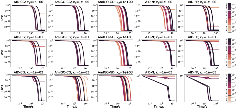
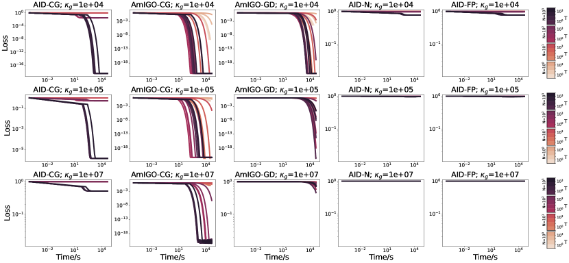
Figure 2: Evolution of the relative error vs. time in seconds for different AID based methods on the synthetic example. Each column corresponds to a method (AID-CG, AmIGO-CG, AmIGO-GD, AID-N, AID-FP) and each row corresponds to a choice of the conditioning number $\kappa_{g}$. For each method we consider $T$ and $N$ from a grid $\{1,10,10^{2},10^{3}\}\times\{1,10,10^{2},10^{3}\}$. Lightest colors corresponds to smaller values of $N$ while nuances within each color correspond to increasing values of $T$.

To study the behavior of AmIGO in a controlled setting, we consider a synthetic problem where both inner and outer level losses are quadratic functions with thousands of variables as described in details in Section F.1. Figure 1(a) shows the complexity $\mathcal{C}(\epsilon)$ needed to reach $10^{-6}$ relative error amongst the best choice for $T$ and $M$ over a grid as the conditioning number $\kappa_{g}$ increases. AmIGO-CG achieves the lowest time and is followed by AID-CG thus showing a favorable effect of warm-start for $\mathcal{B}_{k}$. The same conclusion holds for AmIGO-GD compared to AID-GD. Note that AID-CG is still faster than AmIGO-CG for larger values of $\kappa_{g}$ highlighting the advantage of using algorithms $\mathcal{B}_{k}$ with $O(\sqrt{\kappa_{g}})$ complexity such as (CG) instead non-accelerated ones with $O(\kappa_{g}^{-1})$ such as (GD). Figure 1(b) shows the relative error after $10$s and maintains the same conclusions. For moderate values of $\kappa_{g}$, only AmIGO and AID-CG reach an error of $10^{-20}$ as shown in Figure 1(c). We refer to Figures 2 and 3 of Appendix F for additional results on the effect of the choice of $T$ and $M$ showing that AmIGO consistently performs well for a wide range of values of $T$ and $M$.

5.2 Hyper-parameter optimization

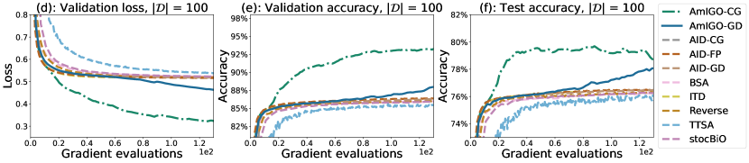
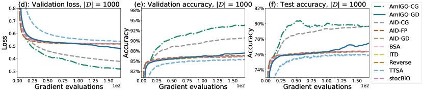
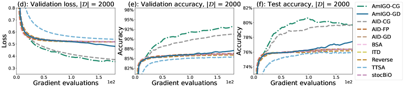
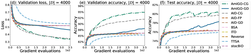
Figure 4: Evolution of the validation loss (left column), validation accuracy (middle column) and test accuracy (right column) in time (s) for different methods on the logistic regression task. Each row correspond to different choices for the size of the batch ${\left\lvert\mathcal{D}\right\rvert}\in\{100,1000,2000,4000\}$ chosen to be the same for all gradient, Hessian and Jacobian-vector products evaluations. Time is reported in seconds.

We consider a classification task on the 20Newsgroup dataset using a logistic loss and a linear model. Each dimension of the linear model is regularized using a different hyper-parameter. The collection of those hyper-parameters form a vector $x$ of dimension $d{=}101631$ optimized using an un-regularized regression loss over the validation set while the model is learned using the training set. We consider two evaluations settings: A default setting based on Grazzi et al. (2020); Ji et al. (2021) and a grid-seach search setting near the default values of $\beta_{k}$, $T$ and $N$ as detailed in Section F.2. We also vary the batch-size from $10^{3}*\{0.1,1,2,4\}$ and report the best performing choices for each method. Figure 1(d,e,f) show AmIGO-CG to be the fastest, achieving the lowest error and highest validation and test accuracies. The test accuracy of AmIGO-CG decreases after exceeding $80\%$ indicating a potential overfitting as also observed in Franceschi et al. (2018). Similarly, AmIGO-GD outperformed all other methods that uses an algorithm $\mathcal{B}_{k}$ with $O(\kappa_{g})$ complexity. Moreover, all remaining methods achieved comparable performance matching those reported in Ji et al. (2021), thus indicating that the warm-start in $\mathcal{B}_{k}$ and acceleration in $\mathcal{B}_{k}$ were the determining factors for obtaining an improved performance. Additionally, Figure 4 of Appendix F report similar results for each choice of the batch-size indicating robustness to the choice of the batch-size.

5.3 Dataset distillation

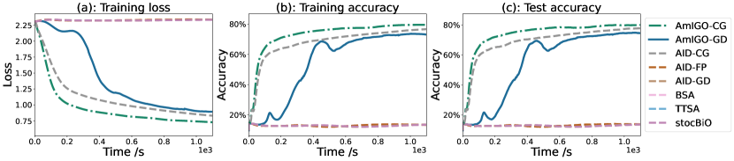
Figure 5: Performance of various bi-level algorithms on the dataset distillation task on MNIST dataset.

Dataset distillation (Wang et al., 2018) consists in learning a synthetic dataset so that a model trained on this dataset achieves a small error on the training set. Figure 5 of Section F.3 shows the training loss (outer loss), the training and test accuracies of a model trained on MNIST by dataset distillation. Similarly to Figure 1, AmIGO-CG achieves the best performance followed by AID-CG. AmIGO obtains the best performance by far among methods without acceleration for $\mathcal{B}_{k}$ while all the remaining ones fail to improve. This finding is indicative of an ill-conditioned inner-level problem as confirmed when computing the conditioning number of the hessian $\partial_{yy}g(x,y)$ which we found to be of order $7{\times}10^{4}$. Indeed, when compared to the synthetic example for $\kappa_{g}{=}10^{4}$ as shown in Figure 2, we also observe that only AmIGO-CG, AmIGO and AID-CG could successfully optimize the loss. Hence, these results confirm the importance of warm-start for an improved performance.

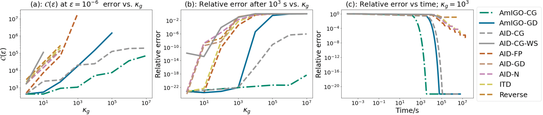
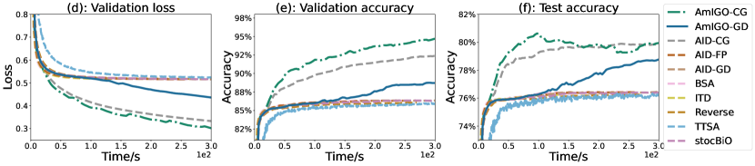
Figure 1: Top row: performance on the synthetic task. The relative error is defined as a ratio between current and initial errors ${\left(\mathcal{L}(x_{k})-\mathcal{L}^{\star}\right)}/{\left(\mathcal{L}(x_{0})-\mathcal{L}^{\star}\right)}$. The complexity $\mathcal{C}(\epsilon)$ as defined in Equation 17. Bottom row: performance on the hyper-parameter optimization task.

6 Conclusion

We studied AmIGO, an algorithm for bilevel optimization based on amortized implicit differentiation and introduced a unified framework for analyzing its convergence. Our analysis showed that AmIGO achieves the same complexity as unbiased oracle methods, thus achieving improved rates compared to methods without warm-start in various settings. We then illustrated empirically such improved convergence in both synthetic and a hyper-optimization experiments. A future research direction consists in extending the proposed framework to non-smooth objectives and analyzing acceleration in both inner and outer level problems as well as variance reduction techniques.

7 Acknowledgments and Funding

This project was supported by the ERC grant number 714381 (SOLARIS project) and by ANR 3IA MIAI@Grenoble Alpes, (ANR19-P3IA-0003).

Appendix A Convergence of AmIGO algorithm

In this section, we provide a proof of Theorem 1 as well as its corollaries Corrolaries 1, 2, 3 and 4. In Section A.1, we provide an outline of the proof Theorem 1 that states the main intermediary results needed for the proof and provide explicit expressions for the quantities needed throughout the rest of the paper. Sections A.2 and A.3 provide the proofs of Theorem 1 and Corrolaries 1, 2, 3 and 4. The proofs of the intermediary results are deferred to Appendices B and C.

A.1 Proof outline of Theorem 1

The proof of Theorem 1 proceeds in 8 steps as discussed bellow.

Step 1: Smoothness properties. This step consists in characterizing the smoothness of $\nabla\mathcal{L}$, $y^{\star}$, $z^{\star}$ as well as the conditional expectation $\mathbb{E}[\hat{\psi}_{k}|x_{k},y_{k},z_{k}]$ knowing $x_{k}$, $y_{k}$ and $z_{k}$. For this purpose, we consider the function $\Psi:\mathcal{X}\times\mathcal{Y}\times\mathcal{Y}\rightarrow\mathcal{X}$ defined as follows:

$$\Psi(x,y,z):=\partial_{x}f(x,y)+\partial_{xy}g(x,y)z.$$ (25)

Hence, by definition of $\hat{\psi}_{k}$, it is easy to see that $\mathbb{E}[\hat{\psi}_{k}|x_{k},y_{k},z_{k}]=\Psi(x_{k},y_{k},z_{k})$. The following proposition controls the smoothness of $\nabla\mathcal{L}$, $y^{\star}$, $z^{\star}$ and $\Psi$ and is adapted from [Ghadimi and Wang, 2018, Lemma 2.2]. We provide a proof in Section B.2 for completeness.

Proposition 6.

Under Assumptions 1, 2 and 3, $\mathcal{L}$, $\Psi$, $y^{\star}$ and $z^{\star}$ satisfy:

$${\left\lVert y^{\star}(x)-y^{\star}(x^{\prime})\right\rVert}\leq L_{y}{\left\lVert x-x^{\prime}\right\rVert},\qquad{\left\lVert z^{\star}(x,y)-z^{\star}(x^{\prime},y^{\prime})\right\rVert}\leq L_{z}{\left({\left\lVert x-x^{\prime}\right\rVert}+{\left\lVert y-y^{\prime}\right\rVert}\right)}$$ (26)

$${\left\lVert\nabla\mathcal{L}(x)-\nabla\mathcal{L}(x^{\prime})\right\rVert}\leq L{\left\lVert x-x^{\prime}\right\rVert},\quad{\left\lVert\Psi(x,y,z)-\nabla\mathcal{L}(x)\right\rVert}\leq L_{\psi}{\left[{\left\lVert y-y^{\star}(x)\right\rVert}+{\left\lVert z-z^{\star}(x,y)\right\rVert}\right]}$$ (27)

$${\left\lVert z^{\star}(x,y^{\star}(x))\right\rVert}\leq\mu_{g}^{-1}B,$$ (28)

where $L_{y}$, $L_{z}$, $L_{\psi}$ and $L$ are given by:

$$L_{y}:=\mu_{g}^{-1}L_{g}^{\prime},\qquad L_{z}:=\mu_{g}^{-2}M_{g}B+\mu_{g}^{-1}L_{f},$$ (29)

$$L_{\psi}:=\max{\left({\left(L_{f}+M_{g}\mu_{g}^{-1}B+L_{g}^{\prime}L_{z}\right)},L_{g}^{\prime}\right)}$$ (30)

$$L:={\left(L_{f}+\mu_{g}^{-2}L_{g}^{\prime}M_{g}B+\mu_{g}^{-1}{\left(L_{g}^{\prime}L_{f}+M_{g}B\right)}\right)}{\left(1+\mu_{g}^{-1}L_{g}^{\prime}\right)}$$ (31)

The expressions of $L_{y}$, $L_{z}$, $L_{\psi}$ and $L$ suggests the following dependence on the conditioning $\kappa_{g}$ of the inner-level problem which will be useful for the complexity analysis: $L_{y}=O(\kappa_{g})$, $L_{\psi}=O(\kappa_{g}^{2})$, $L_{z}=O(\kappa_{g}^{2})$ and $L=O(\kappa_{g}^{3})$.

Step 2: Convergence of the inner-level iterates. In this step, we control the mean squared errors $\mathbb{E}{\left[{\left\lVert y_{k}-y^{\star}(x_{k})\right\rVert}^{2}\right]}$ and $\mathbb{E}{\left[{\left\lVert z_{k}-z^{\star}(x_{k},y_{k})\right\rVert}^{2}\right]}$ as stated in Proposition 3. In fact we prove a slightly stronger version stated below:

Proposition 7.

Let $\alpha_{k}$ and $\beta_{k}$ be two positive sequences with $\alpha_{k}{\leq}L_{g}^{-1}$ and $\beta_{k}{\leq}\frac{1}{2L_{g}}\min{\left(1,\frac{2L_{g}}{\mu_{g}(1+\mu_{g}^{-2}\sigma_{g_{yy}}^{2})}\right)}$ and define $\Lambda_{k}{:=}{\left(1{-}\alpha_{k}\mu_{g}\right)}^{T}$ and $\Pi_{k}{:=}{\left(1{-}\frac{\beta_{k}\mu_{g}}{2}\right)}^{N}$. Denote by $\bar{z}_{k}$ the conditional expectation of $z_{k}$ knowing $x_{k}$, $y_{k}$ and $z_{k}^{0}$. Let $R_{k}^{y}$ and $R_{k}^{z}$ be defined as:

$$R_{k}^{y}:=2\alpha_{k}\mu_{g}^{-1}\sigma_{g}^{2},\quad R_{k}^{z}:=\beta_{k}B^{2}\mu_{g}^{-3}\sigma_{g_{yy}}^{2}+3\mu_{g}^{-2}\sigma_{f}^{2}.$$ (32)

Then, under Assumptions 1, 4 and 5 the iterates $z_{k}$ and $\bar{z}_{k}$ satisfy:

$$\mathbb{E}{\left[{\left\lVert y_{k}-y^{\star}(x_{k})\right\rVert}^{2}\right]}\leq\Lambda_{k}E_{k}^{y}+R_{k}^{y}$$ (33a)

$$\mathbb{E}{\left[{\left\lVert z_{k}-z^{\star}(x_{k},y_{k})\right\rVert}^{2}\right]}\leq\Pi_{k}\mathbb{E}{\left[{\left\lVert z_{k}^{0}-z^{\star}(x_{k},y_{k})\right\rVert}^{2}\right]}+R_{k}^{z},$$ (33b)

$$\mathbb{E}{\left[{\left\lVert\bar{z}_{k}-z^{\star}(x_{k},y_{k})\right\rVert}^{2}\right]}\leq\Pi_{k}\mathbb{E}{\left[{\left\lVert z_{k}^{0}-z^{\star}(x_{k},y_{k})\right\rVert}^{2}\right]}$$ (33c)

$$\mathbb{E}{\left[{\left\lVert z_{k}-\bar{z}_{k}\right\rVert}^{2}\right]}\leq 4\sigma_{g}^{2}\mu_{g}^{-2}\Pi_{k}\mathbb{E}{\left[{\left\lVert z_{k}^{0}-z^{\star}(x_{k},y_{k})\right\rVert}^{2}\right]}+2R_{k}^{z}.$$ (33d)

It is easy to see from the above expressions that $R_{k}^{y}=O{\left(\kappa_{g}\sigma_{g}^{2}\right)}$ while $R_{k}^{z}=O{\left(\kappa_{g}^{3}\sigma_{g_{y}y}^{2}+\kappa_{g}^{2}\sigma_{f}^{2}\right)}$ as stated in Proposition 3. Controlling $\mathbb{E}{\left[{\left\lVert y_{k}-y^{\star}(x_{k})\right\rVert}\right]}^{2}$ follows by standard results on SGD [Kulunchakov and Mairal, 2020, Corollary 31] since the iterates of Algorithm 2 uses i.i.d. samples. The error terms $\mathbb{E}{\left[{\left\lVert z_{k}-z^{\star}(x_{k},y_{k})\right\rVert}^{2}\right]}$ is more delicate since Algorithm 3 uses the same sample $\partial_{y}\hat{f}(x_{k},y_{k})$ for updating the iterates, therefore introducing additional correlations between these iterates. We defer the proof of Proposition 7 to Section B.3 which relies on a general result for stochastic linear systems with correlated noise provided in Appendix E.

Step 3: Controlling the bias and variance errors $V_{k}^{\psi}$ and $E_{k}^{\psi}$ is achieved by Proposition 4. The bias $E_{k}^{\psi}$ is controlled simply by using the smoothness of the potential $\Psi$ near the point $(x_{k},y^{\star}(x_{k}),z^{\star}(x_{k},y^{\star}(x_{k}))$ as shown in Proposition 6. The variance term $V_{k}^{\psi}$ is more delicate to control due to the multiplicative noise resulting from the Jacobian-vector product between $\partial_{xy}\hat{g}(x_{k},y_{k},\mathcal{D}_{g_{xy}})z_{k}$. We defer the proof to Section B.4 and provide below explicit expressions for the constants $\sigma_{x}^{2}$ and $w_{x}^{2}$:

$$w_{x}^{2}:= {\left(1+2L_{g}^{\prime}\mu_{g}^{-1}+6{\left(\sigma_{g_{xy}}^{2}+(L_{g}^{\prime})^{2}\right)}\mu_{g}^{-2}\right)}\sigma_{f}^{2}$$ (34a)

$$+2{\left(\sigma_{g_{xy}}^{2}+(L_{g}^{\prime})^{2}\right)}B^{2}L_{g}^{-1}\mu_{g}^{-3}\sigma_{g_{yy}}^{2}+2B^{2}\mu_{g}^{-2}\sigma_{g_{xy}}^{2}.$$ (34b)

$$\sigma_{x}^{2}:= 2\sigma_{g_{xy}}^{2}+2(L_{g}^{\prime})^{2}\mu_{g}^{-2}\sigma_{g_{yy}}^{2}.$$ (34c)

Note that $w_{x}^{2}{=}O{\left(\kappa_{g}^{2}{\left(\sigma_{f}^{2}+\sigma_{g_{xy}}^{2}\right)}{+}\kappa_{g}^{3}\sigma_{g_{yy}}^{2}\right)}$ and $\sigma_{x}^{2}{=}O{\left(\sigma_{g_{xy}}^{2}{+}\kappa_{g}^{2}\sigma_{g_{yy}}^{2}\right)}$, as stated in Proposition 4.

Step 4: Outer-level error bound. This step consists in obtaining the inequality in Proposition 2 which extends the result of [Kulunchakov and Mairal, 2020, Proposition 1] to biased gradients and to the non-convex case. We defer the proof of such result to Section C.1.

Step 5: Inner-level error bound. This step consists in proving Proposition 5. For clarity, we provide a second statement with explicit expressions for the quantities of interest:

Proposition 8.

Let $r_{k}$ and $\theta_{k}$ be two positive non-increasing sequences no greater than $1$. For any $0\leq v\leq 1$, denote by $\phi_{k}$ and $\tilde{R}_{k}$ the following non-negative scalars:

$$\phi_{k}:=(1-v)L_{g}^{2}T^{2}\alpha_{k}^{2}+2v,\qquad\tilde{R}^{y}_{k}:=2(1-v)L_{g}\mu_{g}^{-1}T^{2}\sigma_{g}^{2}\alpha_{k}^{2}+vR_{k}^{y}$$ (35)

$$\zeta_{k}:=2L{\left(\min{\left((1-u)^{-1},L\eta_{k-1}^{-1}\right)}\mathds{1}_{\mu\geq 0}+\mathds{1}_{\mu<0}\right)}$$ (36)

Finally, consider the following matrices and vectors:

$$\boldsymbol{P_{k}}:=\begin{pmatrix}1+r_{k},&0\\ 16L_{z}^{2}\frac{\phi_{k}}{\theta_{k}},&1+\theta_{k}\end{pmatrix},\quad\boldsymbol{U_{k}}:=\begin{pmatrix}2L_{y}^{2}\frac{\gamma_{k}}{r_{k}}\\ 4L_{z}^{2}\frac{\gamma_{k}}{\theta_{k}}{\left(1+4L_{y}^{2}\frac{\phi_{k}}{r_{k}}\right)}\end{pmatrix},\quad\boldsymbol{V_{k}}:=\tilde{R}^{y}_{k}\begin{pmatrix}0\\ 8L_{z}^{2}\theta_{k}^{-1}\end{pmatrix}.$$ (37)

Then, under Assumptions 1, 2, 3, 4 and 5, the following holds:

$$\begin{pmatrix}E_{k}^{y}\\ E_{k}^{z}\end{pmatrix}\leq\boldsymbol{P_{k}}\begin{pmatrix}\Lambda_{k-1}E_{k-1}^{y}+R_{k-1}^{y}\\ \Pi_{k-1}E_{k-1}^{z}+R_{k-1}^{z}\end{pmatrix}+2\gamma_{k}{\left(E_{k-1}^{\psi}+V_{k-1}^{\psi}+\zeta_{k}E_{k-1}^{x}\right)}\boldsymbol{U_{k}}+\boldsymbol{V_{k}}.$$ (38)

We defer the proof of the above result to Section C.2.

Step 6: General error bound. By combining the inequalities in Propositions 2 and 8 resulting from the analysis of both outer and inner levels, we obtain a general error bound on $E_{k}^{tot}$ in Proposition 9 with a proof in Section C.4.

Proposition 9.

Choose the step-sizes $\alpha_{k}$ and $\beta_{k}$ such that they are non-increasing in $k$ and choose $r_{k}$ and $\theta_{k}$ such that $\delta_{k}r_{k}^{-1}$ and $\delta_{k}\theta_{k}^{-1}$ are non-increasing sequences. Choose the coefficients $a_{k}$ and $b_{k}$ defining $E_{k}^{tot}$ in Equation 14 to be of the form $a_{k}=\delta_{k}r_{k}^{-1}\Lambda_{k}^{s}$ and $b_{k}=\delta_{k}\theta_{k}^{-1}\Pi_{k}^{s}$ for some $0<s<1$. and fix a non-increasing sequence $0<\rho_{k}<1$. Then, under Assumptions 1, 2, 3, 4 and 5 $E_{k}^{tot}$ satisfies:

$$F_{k}+E_{k}^{tot}\leq{\left\lVert A_{k}\right\rVert}_{\infty}E_{k-1}^{tot}+V_{k}^{tot}.$$ (39)

where $V_{k}$ and $\boldsymbol{A_{k}}$ are given by:

$$A_{k}:= \begin{pmatrix}1-(1-\frac{1}{2}\rho_{k})\delta_{k}+2\zeta_{k}\lambda_{k}u_{k}^{I}\\ \Lambda_{k}^{1-s}{\left(1+r_{k}{\left(1+16L_{z}^{2}\Pi_{k}^{s}\theta_{k}^{-2}\phi_{k}+2L_{\psi}^{2}\eta_{k}^{-1}{\left(2u_{k}^{I}+s_{k}+\rho_{k}^{-1}\right)}\right)}\right)}\\ \Pi_{k}^{1-s}{\left(1+\theta_{k}{\left(1+\eta_{k}^{-1}{\left(2L_{\psi}^{2}+\sigma_{x}^{2}\right)}{\left(2u_{k}^{I}+s_{k}+\rho_{k}^{-1}\right)}\right)}\right)}\end{pmatrix}$$ (40)

$$V_{k}^{tot}:= \delta_{k}{\left(\Lambda_{k}^{s}(1+r_{k}^{-1})+16L_{z}^{2}\phi_{k}\theta_{k}^{-2}\Pi_{k}^{s}+2L_{\psi}^{2}\eta_{k}^{-1}{\left(2u_{k}^{I}+s_{k}+\rho_{k}^{-1}\right)}\right)}R_{k-1}^{y}$$ (41)

$$+\delta_{k}{\left((1+\theta_{k}^{-1})\Pi_{k}^{s}R_{k-1}^{z}+8L_{z}^{2}\theta_{k}^{-2}\Pi_{k}^{s}\tilde{R}_{k}^{y}\right)}+\gamma_{k}{\left(s_{k}+u_{k}^{I}\right)}w_{x}^{2}$$ (42)

where we introduced $u_{k}^{I}=a_{k}U_{k}^{(1)}+b_{k}U_{k}^{(2)}$ for conciseness with $U_{k}^{(1)}$ and $U_{k}^{(2)}$ being the components of the vector $\boldsymbol{U_{k}}$ defined in Proposition 8.

Proposition 9 holds without conditions on the error made by Algorithms 3 and 2. The general form of $a_{k}$ and $b_{k}$ allows to account for potentially decreasing step-sizes $\gamma_{k}$, $\alpha_{k}$ and $\beta_{k}$. However, in the present work, we will restrict to the constant step-size for ease of presentation as we discuss next.

Step 7: Controlling the precision of the inner-level algorithms. In this step, we provide conditions on $T$ and $N$ in Proposition 10 bellow so that ${\left\lVert A_{k}\right\rVert}_{\infty}\leq 1-(1-\rho_{k})\delta_{k}$ in the constant step-size case. These conditions are expressed in terms of the following constants:

$$C_{1}:= 1+2\log{\left(6+24L_{\psi}^{2}\eta_{0}^{-1}\right)}$$ (43a)

$$C_{2}:= 2\log{\left(1+4L_{y}^{2}L^{-2}\max{\left(\eta_{0},8\zeta_{0}\right)}\right)}$$ (43b)

$$C_{3}:= \max{\left(0,-2\log{\left(5L_{\psi}^{2}\eta_{0}^{-1}\right)},-2\log{\left(\frac{L}{4L_{y}^{2}}\right)}\right)}$$ (43c)

$$C_{1}^{\prime}:= 1+2\log{\left(4+12\eta_{0}^{-1}(2L_{\psi}^{2}+\sigma_{x}^{2})\right)}$$ (43d)

$$C_{2}^{\prime}:= 2\log{\left(1+2L_{z}^{2}L_{y}^{-2}{\left(1+16L_{y}^{2}\right)}\right)},$$ (43e)

$$C_{3}^{\prime}:= \max{\left(0,-2\log{\left(\frac{L_{\psi}^{2}}{4L_{z}^{2}\eta_{0}}\right)},-2\log{\left(\gamma{\left(\sigma_{g_{xy}}^{2}+(L_{g}^{\prime})^{2}\right)}\right)}\right)}$$ (43f)

Proposition 10.

Let Assumptions 1, 2, 3, 4 and 5 hold. Choose $\rho_{k}=\frac{1}{2}$, the step-sizes to be constant: $\alpha_{k}{=}\alpha{\leq}\frac{1}{L_{g}}$, $\beta_{k}{=}\beta{\leq}\frac{1}{2L_{g}}$ and $\gamma_{k}{=}\gamma{\leq}\frac{1}{L}$ and choose the batch-size ${\left\lvert\mathcal{D}_{g_{yy}}\right\rvert}=\Theta{\left(\frac{\tilde{\sigma}^{2}_{g_{yy}}}{\mu_{g}L_{g}}\right)}$. Moreover, set $s=\frac{1}{2}$, $r_{k}=\theta_{k}=1$. Finally, choose $T$ and $N$ as follows:

$$T=\lfloor\alpha^{-1}\mu_{g}^{-1}\max{\left(C_{1},C_{2},C_{3}\right)}\rfloor+1,$$ (44)

$$N=\lfloor 2\beta^{-1}\mu_{g}^{-1}{\left(\max{\left(C_{1},C_{2},C_{3}\right)}+\max{\left(C_{1}^{\prime},C_{2}^{\prime},C_{3}^{\prime}\right)}\right)}\rfloor+1$$ (45)

with $C_{1},C_{2},C_{3},C_{1}^{\prime},C_{2}^{\prime}$ and $C_{3}^{\prime}$ defined in Equations 43a, 43d, 43b, 43e, 43c and 43f. Then, ${\left\lVert A_{k}\right\rVert}_{\infty}\leq 1-(1-\rho_{k})\delta_{k}$ and $V_{k}^{tot}\leq\gamma\delta_{0}\mathcal{W}^{2}$, with $\mathcal{W}^{2}$ given by:

$$\mathcal{W}^{2}:={\left(\delta_{0}^{-1}\frac{1-u}{2}\mathds{1}_{\mu>0}+3\right)}w_{x}^{2}+\frac{60L_{\psi}^{2}}{\delta_{0}\mu_{g}L_{g}}\sigma_{g}^{2}$$ (46)

We provide a proof of Proposition 10 in Appendix D. It is easy to see from Proposition 10 that that $T{=}O{\left(\kappa_{g}\right)}$ and $N{=}O{\left(\kappa_{g}\right)}$ when $\alpha{=}\frac{1}{L_{g}}$ and $\beta{=}\frac{1}{2L_{g}}$, where the big-$O$ notation hides a logarithmic dependence in $\kappa_{g}$ coming from the constants $\{C_{i},C_{i}^{\prime}|i\in\{1,2,3\}\}$.

Step 8: Proving the main inequalities. The final step combines Propositions 9 and 10 to get the desired inequality. We provide a full proof in Section A.2 assuming Propositions 9 and 10 hold.

A.2 Proof of Theorem 1

In order to prove Theorem 1 in the convex case, we need the following averaging strategy lemma, a generalization of [Kulunchakov and Mairal, 2020, Lemma 30]:

Lemma 1.

Let $\mathcal{L}$ be a convex function on $\mathcal{X}$. Let $x_{k}$ be a (potentially stochastic) sequence of iterates in $\mathcal{X}$. Let $(E_{k})_{k\geq 0}$ , $(V_{k})_{k\geq 0}$ and $(\delta_{k})_{k\geq 0}$ be non-negative sequences such that $\delta_{k}\in(0,1)$. Fix some non-negative number $u\in[0,1]$ and define the following averaged iterates $\hat{x}_{k}$ recursively by $\hat{x}_{k}=u(1-\delta_{k})\hat{x}_{k-1}+{\left(1-(1-\delta_{k})u\right)}x_{k}$ and starting from any initial point $\hat{x}_{0}$. Assume the iterates $(x_{k})_{k\geq 1}$ satisfy the following relation for all $k\geq 1$:

$${\left(1-u(1-\delta_{k})\right)}\mathbb{E}{\left[\mathcal{L}(x_{k})-\mathcal{L}^{\star}\right]}+E_{k}\leq(1-\delta_{k}){\left(E_{k-1}+(1-u)\mathbb{E}{\left[\mathcal{L}(x_{k-1})-\mathcal{L}^{\star}\right]}\right)}+V_{k}.$$ (47)

Let $\Gamma_{k}:=\prod_{t=1}^{k}(1-\delta_{k})$. Then the averaged iterates $(\hat{x}_{k})_{k\geq 1}$ satisfy the following:

$$\mathbb{E}{\left[\mathcal{L}(\hat{x}_{k})-\mathcal{L}^{\star}\right]}+E_{k}\leq\Gamma_{k}{\left(E_{0}+\mathbb{E}{\left[\mathcal{L}(x_{0})-\mathcal{L}^{\star}+u^{k}{\left(\mathcal{L}(\hat{x}_{0})-\mathcal{L}^{\star}\right)}\right]}\right)}+\Gamma_{k}\sum_{1\leq t\leq k}\Gamma_{t}^{-1}V_{t}.$$ (48)

Proof.

For simplicity, we write $F_{k}=\mathbb{E}{\left[\mathcal{L}(x_{k})-\mathcal{L}^{\star}\right]}$ and $\hat{F}_{k}=\mathbb{E}{\left[\mathcal{L}(\hat{x}_{k})-\mathcal{L}^{\star}\right]}$. We first multiply Equation 47 by $\Gamma_{k}^{-1}$ and sum the resulting inequalities for all $1\leq k\leq K$ to get:

$$\sum_{k=1}^{K}\Gamma_{k}^{-1}{\left(1-u(1-\delta_{k})\right)}F_{k}+\Gamma_{k}^{-1}T_{k}\leq\sum_{k=1}^{K}\Gamma_{k}^{-1}(1-\delta_{k}){\left(T_{k-1}+(1-u)F_{k-1}\right)}+\sum_{k=1}^{K}\Gamma_{k}^{-1}V_{k}.$$ (49)

Grouping the terms in $F_{k}$ together and recalling that $\Gamma_{k}^{-1}(1-\delta_{k})=\Gamma_{k-1}^{-1}$ yields:

$$\sum_{k=1}^{K}\Gamma_{k}^{-1}F_{k}-\Gamma_{k-1}^{-1}F_{k-1}+u\sum_{k=1}^{K}\Gamma_{k-1}^{-1}{\left(F_{k-1}-F_{k}\right)}\leq\sum_{k=1}^{K}{\left(\Gamma_{k-1}^{-1}T_{k-1}-\Gamma_{k}^{-1}T_{k}\right)}+\sum_{k=1}^{K}\Gamma_{k}^{-1}V_{k}.$$ (50)

Simplifying the telescoping sums and multiplying by $\Gamma_{k}$, we get:

$$F_{K}+u\Gamma_{K}\sum_{k=1}^{K}\Gamma_{k-1}^{-1}{\left(F_{k-1}-F_{k}\right)}\leq-T_{K}+\Gamma_{K}{\left(F_{0}+T_{0}+\sum_{k=1}^{K}\Gamma_{k}^{-1}V_{k}\right)}.$$ (51)

Consider now the quantity $\hat{F}_{k}$. Recalling that $\mathcal{L}$ is convex and by definition of the iterates $\hat{x}_{k}$ we apply Jensen’s inequality to write:

$$\hat{F}_{k}\leq u(1-\delta_{k})\hat{F}_{k-1}+(1-u(1-\delta_{k}))F_{k}.$$ (52)

By iteratively applying the above inequality, we get that:

$$\hat{F}_{K}\leq u^{K}\Gamma_{K}\hat{F}_{0}+\Gamma_{K}\sum_{k=1}^{K}u^{K-k}\Gamma_{k}^{-1}{\left(1-u(1-\delta_{k})\right)}F_{k}$$ (53)

$$= u^{K}\Gamma_{K}\hat{F}_{0}+\Gamma_{K}\sum_{k=1}^{K}u^{K-k}\Gamma_{k}^{-1}F_{k}-\sum_{k=1}^{K}u^{K-k+1}\Gamma_{k-1}F_{k}$$ (54)

$$= u^{K}\Gamma_{K}\hat{F}_{0}+F_{K}+\Gamma_{K}\sum_{k=1}^{K-1}u^{K-k}\Gamma_{k}^{-1}{\left(F_{k}-F_{k+1}\right)}$$ (55)

We can therefore apply Equation 51 to the above inequality to get the desired result. ∎

We now proceed to prove Theorem 1.

Proof of Theorem 1.

By application of Proposition 9 and using the choice of $T$ and $N$ given by Proposition 10, the following inequality holds:

$$F_{k}+E_{k}^{tot}\leq{\left(1-(1-\rho_{k})\delta_{k}\right)}E_{k-1}^{tot}+\gamma\delta_{0}\mathcal{W}^{2}.$$ (56)

with $\mathcal{W}$ defined in Proposition 10. We then distinguish two cases depending on the sign of $\mu$:

Case $\mu\geq 0$. Recall that $F_{k}$ and $E_{k}^{x}$ are given by:

$$F_{k}=u\delta_{k}\mathbb{E}{\left[\mathcal{L}(x_{k})-\mathcal{L}^{\star}\right]},\qquad E_{k}^{x}=\frac{\delta_{k}}{2\gamma_{k}}{\left\lVert x_{k}-x^{\star}\right\rVert}^{2}+(1-u)\mathbb{E}{\left[\mathcal{L}(x_{k})-\mathcal{L}^{\star}\right]}$$ (57)

Since $\mu>0$, $\mathcal{L}$ is a convex function and we can apply Lemma 1 with $V_{k}{=}\gamma\delta_{0}\mathcal{W}^{2}$ and $E_{k}{=}\frac{\delta_{k}}{2\gamma_{k}}{\left\lVert x_{k}-x^{\star}\right\rVert}^{2}{+}a_{k}E_{k}^{y}{+}b_{k}E_{k}^{z}$. The result follows by noting that $\Gamma_{k}\sum_{t=1}^{k}\Gamma_{t}^{-1}\leq\delta_{0}^{-1}$.

Case $\mu<0$. In this case, we recall that $F_{k}$ and $E_{k}^{x}$ are given by:

$$F_{k}=\mathbb{E}{\left[\mathcal{L}(x_{k})-\mathcal{L}(x_{k-1})\right]}+E_{k-1}^{x}-E_{k}^{x},\qquad E_{k}^{x}=L^{-1}\mathbb{E}{\left[{\left\lVert\nabla\mathcal{L}(x_{k})\right\rVert}^{2}\right]}.$$ (58)

We then sum Equation 56 for all iterations $0\leq t\leq k$ which, by telescoping, yields:

$$\mathbb{E}{\left[\mathcal{L}(x_{k})-\mathcal{L}(x_{0})\right]}+E_{0}^{x}-E_{k}^{x}+E_{k}^{tot}-E_{0}^{tot}+\sum_{1\leq t\leq k}(1-\rho_{t})\delta_{t}E_{t}^{tot}\leq k\gamma\delta_{0}\mathcal{W}^{2}.$$ (59)

Using that $\mathbb{E}{\left[\mathcal{L}(x_{k})-\mathcal{L}^{\star}\right]}+E_{k}^{tot}-E_{k}^{x}$ is non-negative since $E_{k}^{tot}-E_{k}^{x}=a_{k}E_{k}^{y}+b_{k}E_{k}^{z}$, we get:

$$\sum_{1\leq t\leq k}(1-\rho_{t})\delta_{t}E_{t}^{x}\leq{\left(\mathbb{E}{\left[\mathcal{L}(x_{0})-\mathcal{L}^{\star}\right]}+a_{0}E_{0}^{y}+b_{0}E_{0}^{z}\right)}+k\gamma\delta_{0}\mathcal{W}^{2}.$$ (60)

Finally, since $\rho_{t}=\frac{1}{2}$, $\delta_{t}=L\gamma$, the result follows after dividing both sides by $\frac{1}{2}kL\gamma$. ∎

A.3 Proof of Corrolaries 1, 2, 3 and 4

Proof of Corollary 1.

Choosing $u=0$ implies that $E_{k}^{x}=\frac{\mu}{2}{\left\lVert x_{k}-x^{\star}\right\rVert}^{2}+\mathcal{L}(x_{k})-\mathcal{L}^{\star}\leq E_{k}^{tot}$. We can then apply Theorem 1 for $\mu>0$ which yields the following:

$$\frac{\mu}{2}{\left\lVert x_{k}-x^{\star}\right\rVert}+\mathcal{L}(x_{k})-\mathcal{L}^{\star}\leq{\left(1-{\left(2\kappa_{\mathcal{L}}\right)}^{-1}\right)}^{k}E_{0}^{tot}+\frac{2\mathcal{W}^{2}}{L}.$$ (61)

In the deterministic setting, it holds all variances vanish : $\sigma_{f}^{2}{=}\sigma_{g}^{2}{=}\sigma_{g_{yy}}^{2}{=}\sigma_{g_{xy}}^{2}{=}0$. Hence, $\mathcal{W}^{2}=0$ by definition of $\mathcal{W}^{2}$. Therefore, to achieve an error $\mathcal{L}(x_{k}){-}\mathcal{L}^{\star}{\leq}\epsilon$ for some $\epsilon{>}0$, Equation 61 suggests choosing $k{=}O{\left(\kappa_{\mathcal{L}}\log{\left(\frac{E_{0}^{tot}}{\epsilon}\right)}\right)}$. Additionally, $T{=}\Theta(\kappa_{g})$ and $N{=}\Theta(\kappa_{g})$ as required by Theorem 1 and since $\sigma_{g_{yy}}^{2}{=}0$, it holds that $N{=}O(\kappa_{g})$. Using batches of size $1$, yields the desired complexity. ∎

Proof of Corollary 2.

Here we choose $u=1$ and apply Theorem 1 for $\mu>0$ which yields:

$$\mathbb{E}{\left[\mathcal{L}(\hat{x}_{k})-\mathcal{L}^{\star}\right]}+E_{k}^{tot}\leq{\left(1-{\left(2\kappa_{\mathcal{L}}\right)}^{-1}\right)}^{k}{\left(E_{0}^{tot}+\mathbb{E}{\left[\mathcal{L}(x_{0})-\mathcal{L}^{\star}\right]}\right)}+2L^{-1}\mathcal{W}^{2}$$ (62)

Hence, to achieve an error $\mathbb{E}{\left[\mathcal{L}(\hat{x}_{k})-\mathcal{L}^{\star}\right]}\leq\epsilon$, we need $k=O{\left(\kappa_{\mathcal{L}}\log{\left(\frac{E_{0}^{tot}+\mathbb{E}{\left[\mathcal{L}(x_{0})-\mathcal{L}^{\star}\right]}}{\epsilon}\right)}\right)}$ to guarantee that the first term in the l.h.s. of the above inequality is $O(\epsilon)$. Moreover, we recall that $L^{-1}=O(\kappa_{g}^{-3})$ from Proposition 6 and that Theorem 1 ensure the variance $\mathcal{W}$ satisfies:

$$\mathcal{W}^{2}= O{\left(\kappa_{g}^{5}\sigma_{g}^{2}+\kappa_{g}^{3}\sigma_{g_{yy}}^{2}+\kappa_{g}^{2}\sigma_{g_{xy}}^{2}+\kappa_{g}^{2}\sigma_{f}^{2}\right)}.$$ (63)

Hence, ensuring the variance term $2L^{-1}\mathcal{W}^{2}$ is of order $\epsilon$ is achieved by choosing the size of the batches as follows:

$${\left\lvert\mathcal{D}_{f}\right\rvert}=\Theta{\left(\frac{\tilde{\sigma}_{f}^{2}}{\epsilon}\right)},\quad{\left\lvert\mathcal{D}_{g}\right\rvert}=\Theta{\left(\frac{\kappa_{\mathcal{L}}\kappa_{g}^{2}\tilde{\sigma}_{g}^{2}}{\epsilon}\right)},\quad{\left\lvert\mathcal{D}_{g_{xy}}\right\rvert}=\Theta{\left(\frac{\tilde{\sigma}_{g_{xy}}^{2}}{\epsilon}\right)},$$ (64)

$${\left\lvert\mathcal{D}_{g_{yy}}\right\rvert}=\Theta{\left(\tilde{\sigma}_{g_{yy}}^{2}{\left(\frac{1}{\epsilon}\vee\kappa_{g}\right)}\right)}$$ (65)

Recall that $T{=}\Theta(\kappa_{g})$ and $N{=}\Theta{\left(\kappa_{g}\right)}$ as required by, Theorem 1, thus yielding the desired result. ∎

Proof of Corollary 3.

In the non-convex deterministic case, recall that $E_{k}^{x}=\frac{1}{L}{\left\lVert\nabla\mathcal{L}(x_{k})\right\rVert}^{2}\leq E_{k}^{tot}$. We thus apply Theorem 1 for $\mu<0$, multiply by $L$ to get:

$$\frac{1}{k}\sum_{t=1}^{k}{\left\lVert\nabla\mathcal{L}(x_{t})\right\rVert}^{2}\leq\frac{2L}{k}{\left(\mathcal{L}(x_{0})-\mathcal{L}^{\star}+{\left(E_{0}^{y}+E_{0}^{z}\right)}\right)}+2\mathcal{W}^{2}.$$ (66)

The setting being deterministic, it holds that $\mathcal{W}^{2}{=}0$. Moreover, recall that $L=O(\kappa_{g}^{3})$ from Proposition 6. Hence, to achieve an error of order $\min_{1\leq t\leq k}{\left\lVert\nabla\mathcal{L}(x_{t})\right\rVert}^{2}\leq\epsilon$, it suffice to choose $k{=}O{\left(\frac{\kappa_{g}^{3}}{\epsilon}{\left(\mathcal{L}(x_{0})-\mathcal{L}^{\star}+{\left(E_{0}^{y}+E_{0}^{z}\right)}\right)}\right)}$. Thus using batches of size $1$ and $T$ and $N$ of order $\kappa_{g}$. ∎

Proof of Corollary 4.

In the non-convex stochastic case, $E_{k}^{x}=\frac{1}{L}\mathbb{E}{\left[{\left\lVert\nabla\mathcal{L}(x_{k})\right\rVert}^{2}\right]}\leq E_{k}^{tot}$. We thus apply Theorem 1 for $\mu<0$, multiply by $L$ to get:

$$\frac{1}{k}\sum_{t=1}^{k}\mathbb{E}{\left[{\left\lVert\nabla\mathcal{L}(x_{t})\right\rVert}^{2}\right]}\leq\frac{2L}{k}{\left(\mathbb{E}{\left[\mathcal{L}(x_{0})-\mathcal{L}^{\star}\right]}+{\left(E_{0}^{y}+E_{0}^{z}\right)}\right)}+2\mathcal{W}^{2}.$$ (67)

to achieve an error of order $\epsilon$, we need to ensure each term in the l.h.s. of the above inequality is of order $\epsilon$. For the first term, similarly to the deterministic setting Corollary 3, we simply need $k=O{\left(\frac{\kappa_{g}^{3}}{\epsilon}{\left(\mathcal{L}(x_{0})-\mathcal{L}^{\star}+{\left(E_{0}^{y}+E_{0}^{z}\right)}\right)}\right)}$. For the second term, we need to have $\mathcal{W}^{2}{=}O(\epsilon)$, which is achieved using the following choice for the sizes of the batches:

$${\left\lvert\mathcal{D}_{f}\right\rvert}=O{\left(\frac{\kappa_{g}^{2}\tilde{\sigma}_{f}^{2}}{\epsilon}\right)},\quad{\left\lvert\mathcal{D}_{g}\right\rvert}=O{\left(\frac{\kappa_{g}^{5}\tilde{\sigma}_{g}^{2}}{\epsilon}\right)},\quad{\left\lvert\mathcal{D}_{g_{xy}}\right\rvert}=O{\left(\frac{\kappa_{g}^{2}\tilde{\sigma}_{g_{xy}}^{2}}{\epsilon}\right)},$$ (68)

$${\left\lvert\mathcal{D}_{g_{yy}}\right\rvert}=O{\left(\frac{\kappa_{g}^{3}\tilde{\sigma}_{g_{yy}}^{2}}{\epsilon}{\left(1\vee\epsilon\mu_{g}^{2}\right)}\right)}.$$ (69)

Finally, as required by Theorem 1, we set $T=\Theta(\kappa_{g})$ and $N=\Theta(\kappa_{g})$ thus yielding the desired complexity. ∎

A.4 Comparaisons with other methods

In this subsection we derive and discuss the complexities of methods presented in Table 1.

A.4.1 Comparaison with TTSA [Hong et al., 2020b]

Proposition 11.

strongly-convex case $\mu>0$. The complexity of the TTSA algorithm in Hong et al. [2020b] to achieve an error $\frac{\mu}{2}\mathbb{E}{\left[{\left\lVert x_{k}-x^{\star}\right\rVert}^{2}\right]}\leq\epsilon$ is given by:

$$\mathcal{C}(\epsilon):=O{\left({\left(\kappa_{g}^{\frac{17}{2}}\kappa_{\mathcal{L}}^{1/2}+\kappa_{\mathcal{L}}^{7/2}\right)}\frac{1}{\epsilon^{\frac{3}{2}}}\log\frac{1}{\epsilon}\right)}$$ (70)

non-convex case $\mu<0$. The complexity of the TTSA algorithm in Hong et al. [2020b] to achieve an error $\frac{1}{k}\sum_{1\leq i\leq k}\mathbb{E}{\left[{\left\lVert\nabla\mathcal{L}(x_{i})\right\rVert}^{2}\right]}\leq\epsilon$ is given by:

$$\mathcal{C}(\epsilon):=k(1+N)=O{\left({\left(\kappa_{g}^{11}+\kappa_{g}^{16}\right)}\frac{1}{\epsilon^{\frac{5}{2}}}\log{\left(\frac{1}{\epsilon}\right)}\right)}.$$ (71)

Proof.

strongly-convex case $\mu>0$ Using the choice of step-sizes in Hong et al. [2020b], the following bound holds:

$$\mathbb{E}{\left[{\left\lVert x_{k}-x^{\star}\right\rVert}^{2}\right]}\lesssim \prod_{i=0}^{k}{\left(1-\frac{8}{3(k+k_{\alpha})}\right)}{\left(\Delta_{x}^{0}+L_{\psi}^{2}\mu_{g}^{-2}\Delta_{0}^{y}\right)}$$ (72)

$$+\frac{L^{2}_{\psi}}{\mu_{g}\mu^{\frac{4}{3}}}{\left(\mu_{g}^{-1}+\frac{\mu_{g}}{\mu^{2}}L^{2}_{y}\right)}{\left(\frac{1}{k+k_{\alpha}}\right)}^{\frac{2}{3}}$$ (73)

where $\Delta_{x}^{0}=\mathbb{E}{\left[{\left\lVert x_{0}-x^{\star}\right\rVert}^{2}\right]}$, $\mathbb{E}{\left[{\left\lVert y_{1}-y^{\star}(x_{0})\right\rVert}^{2}\right]}$ and $k_{\alpha}$ given by:

$$k_{\alpha}=\max{\left(35{\left(\frac{L_{g}^{3}}{\mu_{g}^{3}}(1+\sigma_{g}^{2})^{\frac{3}{2}}\right)},\frac{(512)^{\frac{3}{2}}L_{\psi}^{2}L_{y}^{2}}{\mu^{2}}\right)}.$$ (74)

By a simple calculation, it is easy to see that $\prod_{i=0}^{k}{\left(1-\frac{8}{3(k+k_{\alpha})}\right)}\leq\frac{(k_{\alpha}-1)^{2}}{(k-1+k_{\alpha})^{2}}$. Moreover, using that $L_{\psi}=O(\mu_{g}^{-2})$, $L_{y}=O(\mu_{g}^{-1})$, we get that

$$\frac{\mu}{2}\mathbb{E}{\left[{\left\lVert x_{k}-x^{\star}\right\rVert}^{2}\right]}\lesssim\frac{(k_{\alpha}-1)^{2}}{(k+k_{\alpha}-1)^{2}}{\left(\mu\Delta_{x}^{0}+\mu\mu_{g}^{-6}\Delta_{0}^{y}\right)}+\mu_{g}^{-6}\mu^{-\frac{1}{3}}{\left(1+\mu^{-2}\right)}{\left(\frac{1}{k+k_{\alpha}}\right)}^{\frac{2}{3}}$$ (75)

Using that $L{=}O(\mu_{g}^{-3})$, we get $\mu_{g}^{-6}\mu^{-\frac{1}{3}}{\left(1+\mu^{-2}\right)}{=}O{\left(\mu_{g}^{-5}\kappa_{\mathcal{L}}^{\frac{1}{3}}+\mu_{g}\kappa_{\mathcal{L}}^{\frac{7}{3}}\right)}$. Hence, to reach an error $\epsilon$, we need to control both terms in the above inequality. This suggests the following condition on $k$ to control the second term which dominates the error:

$$k\geq{\left(\mu_{g}^{\frac{3}{2}}\kappa_{\mathcal{L}}^{7/2}+\kappa_{\mathcal{L}}^{1/2}\mu_{g}^{-\frac{15}{2}}\right)}\frac{1}{\epsilon^{\frac{3}{2}}}.$$ (76)

Moreover, the result in [Hong et al., 2020b, Theorem 1] requires $N=\Theta{\left(\kappa_{g}\log\frac{1}{\epsilon}\right)}$, where $N$ is the number of terms in the Neumann series used to approximate the hessian inverse $(\partial_{yy}g(x,y))^{-1}$ in the expression of the gradient $\nabla\mathcal{L}$. Hence, the total complexity is given by the following expression:

$$\mathcal{C}(\epsilon):=k{\left(1+N\right)}=O{\left({\left(\kappa_{g}^{\frac{17}{2}}\kappa_{\mathcal{L}}^{1/2}+\kappa_{\mathcal{L}}^{7/2}\right)}\frac{1}{\epsilon^{\frac{3}{2}}}\log\frac{1}{\epsilon}\right)}$$ (77)

Smooth Non-convex case $\mu<0$. Following Hong et al. [2020b], consider the proximal map of $\mathcal{L}$ for a fixed $\rho>0$:

$$\hat{x}(z):=\arg\min_{x\in\mathcal{X}}{\left\{\mathcal{L}(x)+\frac{\rho}{2}{\left\lVert x-z\right\rVert}^{2}\right\}}$$ (78)

and define the quantity $\tilde{\Delta}_{x}^{k}:=\mathbb{E}{\left[{\left\lVert\hat{x}(x_{k})-x_{k}\right\rVert}^{2}\right]}$, where $x_{k}$ are the iterates produced by the TTSA algorithm. Let $K$ be a random variable uniformly distributed on $\{0,...,K-1\}$ and independent from the remaining r.v. used in the TTSA algorithm. The result in [Hong et al., 2020b, Theorem 2] provide the following error bound on $\tilde{\Delta}_{x}^{k}$

$$\frac{1}{k}\sum_{1\leq i\leq k}\tilde{\Delta}_{x}^{i}\lesssim{\left(L_{\psi}^{2}{\left(\Delta^{0}+\frac{\sigma_{g}^{2}}{\mu_{g}^{2}}\right)}+\mu_{g}\right)}\frac{k^{-\frac{2}{5}}}{L^{2}}.$$ (79)

where $\rho$ is set to $2L$ and $\Delta^{0}{\leq}\max{\left(\mathbb{E}{\left[\mathcal{L}(x_{0}){-}\mathcal{L}^{\star}\right]},\mathbb{E}{\left[{\left\lVert y_{1}{-}y^{\star}(x_{0})\right\rVert}^{2}\right]}\right)}$. Now, recall that by definition of the proximal map, we have the following identity:

$$\frac{1}{k}\sum_{1\leq i\leq k}\mathbb{E}{\left[{\left\lVert\nabla\mathcal{L}(x_{i})\right\rVert}^{2}\right]}\leq 2(\rho^{2}+L^{2})\frac{1}{k}\sum_{1\leq i\leq k}\tilde{\Delta}_{x}^{i}\lesssim L^{2}\frac{1}{k}\sum_{1\leq i\leq k}\tilde{\Delta}_{x}^{i}.$$ (80)

Hence, we obtain the following error bound:

$$\frac{1}{k}\sum_{1\leq i\leq k}\mathbb{E}{\left[{\left\lVert\nabla\mathcal{L}(x_{i})\right\rVert}^{2}\right]}\leq{\left(\kappa_{g}^{4}{\left(\Delta^{0}+\kappa_{g}^{2}\sigma_{g}^{2}\right)}+\mu_{g}\right)}k^{-\frac{2}{5}}$$ (81)

where we used that $L_{\psi}=O(\kappa_{g}^{2})$. Therefore, to reach an error of order $\epsilon$, TTSA requires:

$$k\geq\frac{1}{\epsilon^{\frac{5}{2}}}{\left(\kappa_{g}^{10}\Delta_{0}^{\frac{5}{2}}+\kappa_{g}^{15}\sigma_{g}^{5}\right)}$$ (82)

Moreover, controlling the bias in the estimation of the gradient requires $N=O(\kappa_{g}\log\frac{1}{\epsilon})$ terms in the Neumann series approximating the hessian. Hence, the total complexity of the algorithm is:

$$\mathcal{C}(\epsilon):=k(1+N)=O{\left({\left(\kappa_{g}^{11}+\kappa_{g}^{16}\right)}\frac{1}{\epsilon^{\frac{5}{2}}}\log{\left(\frac{1}{\epsilon}\right)}\right)}.$$ (83)

∎

A.4.2 Comparaison with AccBio [Ji and Liang, 2021]

Complexity of AccBio. The bilevel algorithm AccBio introduced in Ji and Liang [2021] uses acceleration for both the inner and outer loops. This allows to obtain the following conditions on $k$, $T$ and $N$ to achieve an $\epsilon$ accuracy:

$$k=O{\left(\kappa_{\mathcal{L}}^{\frac{1}{2}}\log\frac{1}{\epsilon}\right)},T=O{\left(\kappa_{g}^{\frac{1}{2}}\right)},N=O{\left(\kappa_{g}^{\frac{1}{2}}\log\frac{1}{\epsilon}\right)}.$$ (84)

Note that, since AccBio do not use a warm-start strategy when solving the linear system, $N$ is required to grow as $\log\frac{1}{\epsilon}$ in order to achieve an $\epsilon$ accuracy. This contributes an additional logarithmic factor to the total complexity so that $\mathcal{C}(\epsilon)=O(\kappa_{\mathcal{L}}^{\frac{1}{2}}\kappa_{g}^{\frac{1}{2}}{\left(\log\frac{1}{\epsilon}\right)}^{2})$. This is by contrast with AmIGO which exploits warm start when solving the linear system and thus only needs a constant number of iterations $N=O(\kappa_{g})$ although the dependence on $\kappa_{g}$ is worse compared to AccBio. However, it is possible to improve such dependence by using acceleration in the inner-level algorithms $\mathcal{A}_{k}$ and $\mathcal{B}_{k}$ as we discuss in Section A.5.1.

Complexity of AccBio as a function of $\mu$ and $\mu_{g}$. The authors choose to report the complexity as a function of $\mu$ and $\mu_{g}$ instead of the conditioning numbers $\kappa_{\mathcal{L}}$ and $\kappa_{g}$. To achieve this, they observe that, under the additional assumption that the hessian $\partial_{yy}g(x,y)$ is constant w.r.t. $y$, the Lipschitz constant $L$ has an improved dependence on $\mu_{g}$: $L=O(\mu_{g}^{-2})$ instead of $L=O(\mu_{g}^{-3})$ in the general case where $\partial_{yy}g(x,y)$ is only Lipschitz in $y$. This allows them to express $\kappa_{\mathcal{L}}=\frac{L}{\mu}=O(\mu_{g}^{-2}\mu^{-1})$ and to report the following complexities in terms of $\mu$ and $\mu_{g}$:

$$\mathcal{C}(\epsilon)=O{\left(\mu^{-\frac{1}{2}}\mu_{g}^{-\frac{3}{2}}{\left(\log\frac{1}{\epsilon}\right)}^{2}\right)}.$$ (85)

Note that, in the general case where $L=O(\mu_{g}^{-3})$, the complexity as a function of $\mu$ and $\mu_{g}$ becomes $O{\left(\mu^{-\frac{1}{2}}\mu_{g}^{-2}{\left(\log\frac{1}{\epsilon}\right)}^{2}\right)}$, while still maintaining the same expression in terms of $\kappa_{\mathcal{L}}$ and $\kappa_{g}$. Hence, using the expression in terms of conditioning allows a more general expression for the complexity that is less sensitive to the specific assumptions on $g$ and is therefore more suitable for comparaison with other results in the literature.

A.5 Choice of the inner-level algorithms $\mathcal{A}_{k}$ and $\mathcal{B}_{k}$.

The choice of $\mathcal{A}_{k}$ and $\mathcal{B}_{k}$ has an impact on the total complexity of the algorithm. We discuss two choices for $\mathcal{A}_{k}$ and $\mathcal{B}_{k}$ which improve the total complexity of AmIGO: Accelerated algorithms (in Section A.5.1) and variance reduced algorithms (in Section A.5.2).

A.5.1 Acceleration of the inner-level for AmIGO

AmIGO could benefit from acceleration in the inner-loop by using standard acceleration schemes Nesterov [2003] for $\mathcal{A}_{k}$ and $\mathcal{B}_{k}$. As a consequence, and using analysis of accelerated algorithms [Nesterov, 2003] in the deterministic setting, the error of the inner-level iterates would satisfy:

$$\mathbb{E}{\left[{\left\lVert y_{k}-y^{\star}(x_{k})\right\rVert}^{2}\right]}\leq\tilde{\Lambda}_{k}E_{k}^{y},\qquad\mathbb{E}{\left[{\left\lVert y_{k}-y^{\star}(x_{k})\right\rVert}^{2}\right]}\leq\tilde{\Pi}_{k}E_{k}^{z}$$ (86)

where $\tilde{\Lambda}_{k}$ and $\tilde{\Pi}_{k}$ are accelerated rates of the form $\tilde{\Lambda}_{k}=O((1-\sqrt{\kappa_{g}})^{T})$ and $\tilde{\Pi}_{k}=O((1-\sqrt{\kappa_{g}})^{N})$. The rest of the proofs are similar provided that $\Lambda_{k}$ and $\Pi_{k}$ are replaced by their accelerated rates $\tilde{\Lambda}_{k}$ and $\tilde{\Pi}_{k}$. This implies that $T$ and $N$ need to be only of order $T=O(\sqrt{\kappa_{g}})$ and $N=O(\sqrt{\kappa_{g}})$ so that the final complexity becomes:

$$\mathcal{C}(\epsilon):=O{\left(\kappa_{\mathcal{L}}\kappa_{g}^{1/2}\log\frac{1}{\epsilon}\right)}.$$ (87)

Note that using conjugate gradient for $\mathcal{B}_{k}$ also enjoys an accelerated convergence rate Shewchuk et al. [1994]. This is confirmed in our experiments of Figure 1 where AmIGO-CG enjoys the fastest convergence.

In order to further improve the dependence on $\kappa_{\mathcal{L}}$ to $\kappa_{\mathcal{L}}^{1/2}$, one would need to use an accelerated scheme when updating the iterates $x_{k}$. The analysis of such scheme along with warm-start would be an interesting direction for future work.

A.5.2 Variance reduced algorithms for $\mathcal{A}_{k}$ and $\mathcal{B}_{k}$

When the inner-level cost function $g$ is a finite average of functions $g(x,y)=\frac{1}{n}\sum_{1\leq i\leq n}g_{i}(x,y)$ empirical average, it is possible to use variance reduced algorithms such as SAG [Schmidt et al., 2017]. If every function $g_{i}$ is $L_{g}$-smooth, then by [Schmidt et al., 2017, Proposition 1], the inner level error becomes:

$$\mathbb{E}{\left[{\left\lVert y_{k}-y^{\star}(x_{k})\right\rVert}^{2}\right]}\lesssim\tilde{\Lambda}_{k}(3E_{k}^{y}+\frac{9}{4}L_{g}^{-2}\sigma_{g}^{2}),$$ (88)

with $\tilde{\Lambda}_{k}={\left(1-\frac{\kappa_{g}}{8n}\right)}^{T}$. This has the advantage that the error due to the variance decays exponentially with the number of iterations $T$. As a consequence, the dependence of the effective variance $\mathcal{W}^{2}$ on the conditioning numbers $\kappa_{\mathcal{L}}$ and $\kappa_{g}$ can be improved to:

$$\mathcal{W}^{2}= O{\left({\left\lvert\mathcal{D}_{g}\right\rvert}^{-1}\tilde{\sigma}_{g}^{2}+\kappa_{g}^{3}{\left\lvert\mathcal{D}_{g_{yy}}\right\rvert}^{-1}\tilde{\sigma}_{g_{yy}}^{2}+\kappa_{g}^{2}{\left\lvert\mathcal{D}_{g_{xy}}\right\rvert}^{-1}\tilde{\sigma}_{g_{xy}}^{2}+\kappa_{g}^{2}{\left\lvert\mathcal{D}_{f}\right\rvert}^{-1}\tilde{\sigma}_{f}^{2}\right)}.$$ (89)

This can be achieved by taking $T=O(n\kappa_{g})$ up to a logarithmic dependence on the condition numbers. As a consequence, the complexity in the strongly convex stochastic setting becomes:

$$\mathcal{C}(\epsilon)=O{\left(\kappa_{\mathcal{L}}{\left(n\tilde{\sigma}_{g}^{2}+\kappa_{g}{\left(1\vee\epsilon\kappa_{g}\right)}\tilde{\sigma}_{g_{yy}}^{2}+\tilde{\sigma}_{g_{xy}}^{2}+\tilde{\sigma}_{f}^{2}\right)}\frac{1}{\epsilon}\log{\left(\frac{E_{0}^{tot}+\mathbb{E}{\left[\mathcal{L}(x_{0})-\mathcal{L}^{\star}\right]}}{\epsilon}\right)}\right)}.$$ (90)

In the non-convex setting, the complexity becomes:

$$\mathcal{C}(\epsilon)=O{\left(\frac{\kappa_{g}^{4}}{\epsilon^{2}}{\left(n\tilde{\sigma}_{g}^{2}+\kappa_{g}^{3}{\left(1\vee\epsilon\mu_{g}^{2}\right)}\tilde{\sigma}_{g_{yy}}^{2}+\kappa_{g}\tilde{\sigma}_{g_{xy}}^{2}+\kappa_{g}\tilde{\sigma}_{f}^{2}\right)}{\left(\mathbb{E}{\left[\mathcal{L}(x_{k})-\mathcal{L}^{\star}\right]}+E_{0}^{y}+E_{0}^{z}\right)}\right)}.$$ (91)

The downside of this approach is the dependence on the number $n$ of functions $g_{i}$ in the total complexity.

Appendix B Preliminary results

B.1 Expression of the gradient

We provide a proof of Proposition 1 which shows that $\mathcal{L}$ is differentiable and provides an expression of its gradient.

Proof.

Assumption 1 ensures that $y\mapsto g(x,y)$ admits a unique minimizer $y^{\star}(x)$ defined as the unique solution to the implicit equation $\partial_{y}g(x,y^{\star}(x))=0$. Moreover, since $g$ is twice continuously differentiable and strongly convex, it follows that $\partial_{yy}g(x,y^{\star}(x))$ is invertible for any $x\in\mathcal{X}$. Therefore the implicit function theorem [Lang, 2012, Theorem 5.9], ensures that $x\mapsto y^{\star}(x)$ is continuously differentiable with Jacobian given by $\nabla y^{\star}(x)=-\partial_{xy}g(x,y^{\star}(x))\partial_{yy}g(x,y^{\star}(x))^{-1}$. Hence, by composition of differentiable functions, $\mathcal{L}$ is also differentiable with gradient given by:

$$\nabla\mathcal{L}(x)=\partial_{x}f(x,y^{\star}(x))-\partial_{xy}g(x,y^{\star}(x))\partial_{yy}g(x,y^{\star}(x))^{-1}\partial_{y}f(x,y^{\star}(x)).$$ (92)

We can thus define $z^{\star}(x,y)=-\partial_{yy}g(x,y)^{-1}\partial_{y}f(x,y)$ to get the desired expression for $\nabla\mathcal{L}(x)$ and note that $z^{\star}$ is the solution to Equation 2. ∎

B.2 Smoothness properties of $\mathcal{L}$, $\mathcal{Y}^{\star}$, $z^{\star}$ and $\Psi$

Proof of Proposition 6.

Lipschitz continuity of $x\mapsto y^{\star}(x)$. By Assumptions 3 and 1, the implicit function theorem [Lang, 2012, Theorem 5.9] ensures $y^{\star}(x)$ is differentiable with Jacobian given by:

$$\nabla y^{\star}(x)=-\partial_{xy}g(x,y^{\star}(x)){\left(\partial_{yy}g(x,y^{\star}(x))\right)}^{-1}.$$ (93)

Moreover, by Assumption 3, we know that $\partial_{y}g(x,y)$ is $L_{g}^{\prime}$-Lipchitz in $x$ for any $y\in\mathcal{Y}$, hence, ${\left\lVert\partial_{xy}g(x,y^{\star}(x))\right\rVert}_{op}$ is upper-bounded by $L_{g}^{\prime}$. Moreover, by Assumption 1, $g$ is $\mu_{g}$-strongly convex in $y$ uniformly on $\mathcal{X}$. Therefore, it holds that ${\left\lVert\partial_{yy}g(x,y^{\star}(x))^{-1}\right\rVert}_{op}\leq\mu_{g}^{-1}$. This allows to deduce that ${\left\lVert\nabla y^{\star}(x)\right\rVert}_{op}\leq\mu_{g}^{-1}L_{g}^{\prime}$, and by application of the fundamental theorem of calculus that:

$${\left\lVert y^{\star}(x)-y^{\star}(x^{\prime})\right\rVert}\leq\mu_{g}^{-1}L_{g}^{\prime}{\left\lVert x-x^{\prime}\right\rVert}.$$ (94)

This shows that $y^{\star}$ is $L_{y}$-Lipschitz continuous with $L_{y}:=\mu_{g}^{-1}L_{g}^{\prime}$.

Lipchitz continuity of $x\mapsto z^{\star}(x,y)$. Let $(x,y)$ and $(x^{\prime},y^{\prime})$ be two points in $\mathcal{X}\times\mathcal{Y}$. Recalling the definition of $z^{\star}(x,y)$ in Proposition 1, it is easy to see that $z^{\star}(x,y)$ admits the following expression:

$$z^{\star}(x,y)=-\partial_{yy}g(x,y)^{-1}\partial_{y}f(x,y).$$ (95)

Recalling the expression of $z^{\star}(x,y)$, the following holds:

$$z^{\star}(x,y)-z^{\star}(x^{\prime},y^{\prime})= \partial_{yy}g(x^{\prime},y^{\prime})^{-1}\partial_{y}f(x^{\prime},y^{\prime})-\partial_{yy}g(x,y)^{-1}\partial_{y}f(x,y)$$ (96)

$$= {\left(\partial_{yy}g(x^{\prime},y^{\prime})^{-1}-\partial_{yy}g(x,y)^{-1}\right)}\partial_{y}f(x^{\prime},y^{\prime})$$ (97)

$$+\partial_{yy}g(x,y)^{-1}{\left(\partial_{y}f(x^{\prime},y^{\prime})-\partial_{y}f(x,y)\right)}$$ (98)

$$= \partial_{yy}g(x^{\prime},y^{\prime})^{-1}{\left(\partial_{yy}g(x,y)-\partial_{yy}g(x^{\prime},y^{\prime})\right)}\partial_{yy}g(x,y)^{-1}\partial_{y}f(x^{\prime},y^{\prime})$$ (99)

$$+\partial_{yy}g(x,y)^{-1}{\left(\partial_{y}f(x^{\prime},y^{\prime})-\partial_{y}f(x,y)\right)}$$ (100)

Hence, by taking the norm of the above quantity a triangular inequality followed by operator inequalities, it follows that:

$${\left\lVert z^{\star}(x,y)-z^{\star}(x^{\prime},y^{\prime})\right\rVert}\leq {\left\lVert H_{2}^{-1}\right\rVert}_{op}{\left\lVert H_{1}-H_{2}\right\rVert}_{op}{\left\lVert H_{1}^{-1}\right\rVert}_{op}{\left\lVert\partial_{y}f(x^{\prime},y^{\prime})\right\rVert}$$ (101)

$$+{\left\lVert H_{1}^{-1}\right\rVert}{\left\lVert\partial_{y}f(x^{\prime},y^{\prime})-\partial_{y}f(x,y)\right\rVert}.$$ (102)

where we introduced $H_{1}=\partial_{yy}g(x,y)$ and $H_{2}=\partial_{yy}g(x^{\prime},y^{\prime})$ for conciseness. Using Assumption 1, we can upper-bound ${\left\lVert H_{1}^{-1}\right\rVert}_{op}$ and ${\left\lVert H_{2}^{-1}\right\rVert}_{op}$ by $\mu_{g}^{-1}$. By Assumption 3, we know that ${\left\lVert H_{1}-H_{2}\right\rVert}_{op}\leq M_{g}{\left\lVert(x,y)-(x^{\prime},y^{\prime})\right\rVert}$. Finally by Assumption 2, we also have that ${\left\lVert\partial_{y}f(x^{\prime},y^{\prime})-\partial_{y}f(x,y)\right\rVert}\leq L_{f}{\left\lVert(x,y)-(x^{\prime},y^{\prime})\right\rVert}$ and that ${\left\lVert\partial_{y}f(x^{\prime},y^{\prime})\right\rVert}\leq B$ ensuring that:

$${\left\lVert z^{\star}(x,y)-z^{\star}(x^{\prime},y^{\prime})\right\rVert}\leq{\left(\mu_{g}^{-2}M_{g}B+\mu_{g}^{-1}L_{f}\right)}{\left\lVert(x,y)-(x^{\prime},y^{\prime})\right\rVert}.$$ (103)

Hence, we conclude that $z^{\star}$ is $L_{z}$-Lipchitz continuous with $L_{z}$ defined as in Equation 29.

boundedness of $z^{\star}(x,y)$ Recalling the expression of $z^{\star}$ in Equation 95, it is easy to see that ${\left\lVert z^{\star}(x,y)\right\rVert}$ is upper-bounded by $\mu_{g}^{-1}B$ since $\partial_{yy}g(x,y)$ is $\mu_{g}$-strongly convex in $y$ by Assumption 1 and $\partial_{y}f(x,y)$ is bounded by $B$ by Assumption 2.

Regularity of $\Psi$.

$$\Psi(x,y,z)-\Psi(x^{\prime},y^{\prime},z^{\prime})= \partial_{x}f(x,y)-\partial_{x}f(x^{\prime},y^{\prime})+\partial_{xy}g(x,y)z-\partial_{xy}g(x^{\prime},y^{\prime})z^{\prime}$$ (104)

$$= \partial_{x}f(x,y)-\partial_{x}f(x^{\prime},y^{\prime})+\partial_{xy}g(x,y){\left(z-z^{\prime}\right)}$$ (105)

$$+{\left(\partial_{xy}g(x,y)-\partial_{xy}g(x^{\prime},y^{\prime})\right)}z^{\prime}.$$ (106)

By taking the norm of the above expression and applying a triangular inequality followed by operator inequalities, it follows that:

$${\left\lVert\Psi(x,y,z)-\Psi(x^{\prime},y^{\prime},z^{\prime})\right\rVert}\leq {\left\lVert\partial_{x}f(x,y)-\partial_{x}f(x^{\prime},y^{\prime})\right\rVert}+{\left\lVert\partial_{xy}g(x,y)\right\rVert}_{op}{\left\lVert z-z^{\prime}\right\rVert}$$ (107)

$$+{\left\lVert\partial_{xy}g(x,y)-\partial_{xy}g(x^{\prime},y^{\prime})\right\rVert}_{op}{\left\lVert z^{\prime}\right\rVert}$$ (108)

$$\leq L_{f}{\left({\left\lVert x-x^{\prime}\right\rVert}+{\left\lVert y-y^{\prime}\right\rVert}\right)}+L_{g}^{\prime}{\left\lVert z-z^{\prime}\right\rVert}$$ (109)

$$+M_{g}{\left\lVert z^{\prime}\right\rVert}{\left({\left\lVert x-x^{\prime}\right\rVert}+{\left\lVert y-y^{\prime}\right\rVert}\right)}.$$ (110)

To get the first term of the last inequality above, we used that $\partial_{x}f$ is $L_{f}$-Lipschitz by Assumption 2. To get the second term, we used that $\partial_{xy}g(x,y)$ is bounded since $\partial_{y}g(x,y)$ is $L_{g}^{\prime}$-Lipschitz by Assumption 3. Finally, for the last term, we used that $\partial_{xy}g(x,y)$ is $M_{g}$-Lipschitz by Assumption 3.

By choosing $x^{\prime}=x$, $y^{\prime}=y^{\star}(x)$ and $z^{\prime}=z^{\star}(x,y^{\star}(x))$, it is easy to see from Proposition 1 that $\Psi(x,y^{\star}(x),z^{\star}(x,y^{\star}(x)))=\nabla\mathcal{L}(x)$. Hence, applying the above inequality yields:

$${\left\lVert\Psi(x,y,z)-\nabla\mathcal{L}(x)\right\rVert}\leq {\left(L_{f}+M_{g}{\left\lVert z^{\star}(x,y^{\star}(x))\right\rVert}\right)}{\left\lVert y-y^{\star}(x)\right\rVert}+L_{g}^{\prime}{\left\lVert z-z^{\star}(x,y^{\star}(x))\right\rVert}$$ (111)

$$\leq {\left(L_{f}+M_{g}{\left\lVert z^{\star}(x,y^{\star}(x))\right\rVert}\right)}{\left\lVert y-y^{\star}(x)\right\rVert}+L_{g}^{\prime}{\left\lVert z-z^{\star}(x,y)\right\rVert}$$ (112)

$$+L_{g}^{\prime}{\left\lVert z^{\star}(x,y)-z^{\star}(x,y^{\star}(x))\right\rVert}$$ (113)

As shown earlier, ${\left\lVert z^{\star}(x,y^{\star}(x))\right\rVert}$ is upper-bounded by $\mu_{g}^{-1}B$, while ${\left\lVert z^{\star}(x,y)-z^{\star}(x,y^{\star}(x))\right\rVert}$ is bounded by $L_{z}{\left\lVert y-y^{\star}(x)\right\rVert}$. This allows to conclude that ${\left\lVert\Psi(x,y,z)-\nabla\mathcal{L}(x)\right\rVert}\leq L_{\psi}$ with $L_{\psi}$ defined in Equation 29.

Lipschitz continuity of $x\mapsto\nabla\mathcal{L}(x)$. We apply Equation 107 with $(y,z)=(y^{\star}(x),z^{\star}(x,y^{\star}(x)))$ and $(y^{\prime},z^{\prime})=(y^{\star}(x^{\prime}),z^{\star}(x,y^{\star}(x^{\prime})))$ which yields:

$${\left\lVert\nabla\mathcal{L}(x)-\nabla\mathcal{L}(x^{\prime})\right\rVert}\leq {\left(L_{f}+M_{g}{\left\lVert z^{\star}(x^{\prime},y^{\star}(x^{\prime}))\right\rVert}\right)}{\left({\left\lVert x-x^{\prime}\right\rVert}+{\left\lVert y^{\star}(x)-y^{\star}(x^{\prime})\right\rVert}\right)}$$ (114)

$$+L_{g}^{\prime}{\left\lVert z^{\star}(x,y^{\star}(x))-z^{\star}(x^{\prime},y^{\star}(x^{\prime}))\right\rVert}$$ (115)

$$\leq {\left(L_{f}+M_{g}\mu_{g}^{-1}B+L_{g}^{\prime}L_{z}\right)}{\left(1+L_{y}\right)}{\left\lVert x-x^{\prime}\right\rVert},$$ (116)

where we used that ${\left\lVert z^{\star}(x^{\prime},y^{\star}(x^{\prime}))\right\rVert}$ is upper-bounded by $\mu_{g}^{-1}B$, $z^{\star}$ is $L_{z}$-Lipschitz and $y^{\star}$ is $L_{y}$-Lipschitz. Hence, $\nabla\mathcal{L}$ is $L$-Lipschitz continuous, with $L$ as given by Equation 29. ∎

B.3 Convergence of the iterates of algorithms $\mathcal{A}_{k}$ and $\mathcal{B}_{k}$

Proof.

Controlling the iterates $y^{t}$ of $\mathcal{A}_{k}$.

Consider a new batch $\mathcal{D}_{g}$ of samples $\xi$. We have by definition of the update equation of $y^{t}$ that:

$${\left\lVert y^{t}-y^{\star}(x_{k})\right\rVert}^{2}= {\left\lVert y^{t-1}-y^{\star}(x_{k})\right\rVert}^{2}+\alpha_{k}^{2}{\left\lVert\partial_{y}\hat{g}{\left(x_{k},y^{t-1},\mathcal{D}_{g}\right)}\right\rVert}^{2}$$ (117)

$$-2\alpha_{k}\partial_{y}\hat{g}{\left(x_{k},y^{t-1},\mathcal{D}_{g}\right)}^{\top}{\left(y^{t-1}-y^{\star}(x_{k})\right)}$$ (118)

Taking the expectation conditionally on $x_{k}$ and $y^{t-1}$, we get:

$$\mathbb{E}{\left[{\left\lVert y^{t}-y^{\star}(x_{k})\right\rVert}^{2}\middle|x_{k},y^{t-1}\right]}= (1-\alpha_{k}\mu_{g}){\left\lVert y^{t-1}-y^{\star}(x_{k})\right\rVert}^{2}$$ (119)

$$+\alpha_{k}^{2}\mathbb{E}{\left[{\left\lVert\partial_{y}\hat{g}{\left(x_{k},y^{t-1},\mathcal{D}_{g}\right)}-\partial_{y}g(x_{k},y^{t-1})\right\rVert}^{2}\middle|x_{k},y^{t-1}\right]}$$ (120)

$$-2\alpha_{k}\partial_{y}g{\left(x_{k},y^{t-1}\right)}^{\top}{\left(y^{t-1}-y^{\star}(x_{k})-\frac{\alpha_{k}}{2}\partial_{y}g(x_{k},y^{t-1})\right)}$$ (121)

$$\leq (1-\alpha_{k}\mu_{g}){\left\lVert y^{t-1}-y^{\star}(x_{k})\right\rVert}^{2}+2\alpha_{k}^{2}\sigma_{g}^{2}$$ (122)

The first line uses that $\partial_{y}\hat{g}{\left(x_{k},y^{t-1},\mathcal{D}_{g}\right)}$ is an unbiased estimator of $\partial_{y}g(x_{k},y^{t-1})$. For the second line, we use Assumption 4 which allows to upper-bound the variance of $\partial_{y}\hat{g}$ by $\sigma_{g}^{2}$. Moreover, since $g$ is convex and $L_{g}$-smooth and since $\alpha_{k}\leq L_{g}^{-1}$, it follows that the last term in the above inequality is non-positive and can thus be upper-bounded by $0$. By unrolling the resulting inequality recursively for $1<t\leq k$, we obtain the desired result.

Controlling the iterates $z^{n}$ of $\mathcal{B}_{k}$. The poof follows by direct application of Proposition 15 with $\beta=\beta_{k}$ and the following choices for $A_{n}$, $A$, $\hat{b}$, $b$:

$$A_{n}= \partial_{yy}\hat{g}(x_{k},y_{k},\mathcal{D}_{g_{yy}}),\qquad \hat{b}= \partial_{y}\hat{f}(x_{k},y_{k},\mathcal{D}_{f})$$ (123)

$$A= \partial_{yy}g(x_{k},y_{k})\qquad b= \partial_{y}f(x_{k},y_{k}).$$ (124)

This directly yields the following inequalities:

$$\mathbb{E}{\left[{\left\lVert z_{k}-z^{\star}(x_{k},y_{k})\right\rVert}^{2}\right]}\leq \tilde{\Pi}_{k}\mathbb{E}{\left[{\left\lVert z_{k}^{0}-z^{\star}(x_{k},y_{k})\right\rVert}^{2}\right]}+\tilde{R}_{k}^{z},$$ (125)

$$\mathbb{E}{\left[{\left\lVert\bar{z}_{k}-z^{\star}(x_{k},y_{k})\right\rVert}^{2}\right]}\leq \tilde{\Pi}_{k}\mathbb{E}{\left[{\left\lVert z_{k}^{0}-z^{\star}(x_{k},y_{k})\right\rVert}^{2}\right]}.$$ (126)

where $\tilde{\Pi}_{k}$ and $\tilde{R}_{k}^{z}$ are given by:

$$\tilde{\Pi}_{k}:=(1-\beta_{k}\mu_{g})^{N},\qquad\tilde{R}_{k}^{z}:=\beta_{k}^{2}{\left(\sigma_{g}^{2}\mathbb{E}{\left[{\left\lVert z^{\star}(x_{k},y_{k})\right\rVert}^{2}\right]}+3{\left(N\wedge\frac{1}{\beta_{k}\mu_{g}}\right)}\sigma_{f}^{2}\right)}{\left(N\wedge\frac{1}{\beta_{k}\mu_{g}}\right)}.$$ (127)

First we have that $\tilde{\Pi}_{k}\leq\Pi_{k}$. Moreover, Proposition 6, we have that ${\left\lVert z^{\star}(x_{k},y_{k})\right\rVert}\leq B\mu_{g}^{-1}$ hence, $\tilde{R}_{k}^{z}\leq R_{k}^{z}$ thus yielding the desired inequalities. Finally Equation 33d also follows similarly using Equation 247 from Proposition 15. ∎

B.4 Controlling the bias and variance $E_{k}^{\psi}$ and $V_{k}^{\psi}$

Proof of Proposition 4 .

Recall that the expressions of $E_{k}^{\psi}$ and $V_{k}^{\psi}$ in Equation 12 involves the conditional expectation $\mathbb{E}_{k}{\left[\hat{\psi}_{k}\right]}$ knowing $x_{k}$, $y_{k}$ and $z_{k-1}$. This can be also expressed using $\Psi$ as follows:

$$\mathbb{E}_{k}{\left[\hat{\psi}_{k}\right]}= \mathbb{E}{\left[\mathbb{E}{\left[\hat{\psi}_{k}|x_{k},y_{k},z_{k}\right]}|x_{k},y_{k},z_{k-1}\right]}$$ (128)

$$= \mathbb{E}{\left[\Psi(x_{k},y_{k},z_{k})|x_{k},y_{k},z_{k-1}\right]}$$ (129)

$$= \mathbb{E}{\left[\Psi(x_{k},y_{k},\mathbb{E}{\left[z_{k}||x_{k},y_{k},z_{k-1}\right]})\right]}$$ (130)

where we used the tower property for conditional expectations in the first line, then the fact that the expectation of $\psi_{k}$ conditionally on $x_{k}$, $y_{k}$ and $z_{k}$ is simply $\Psi(x_{k},y_{k},z_{k})$. Finally, for the last line, we use the independence of the noise and the linearity of $\Psi$ w.r.t. the last variable. In all what follows, we write $\bar{z}_{k}=\mathbb{E}{\left[z_{k}|x_{k},y_{k},z_{k-1}\right]}$ which is the same object as defined in Proposition 7. We then treat $E_{k}^{\psi}$ and $V_{k}^{\psi}$ separately.

Bounding $E_{k}^{\psi}$. Using Propositions 7 and 6 we directly get the desired inequality:

$$E_{k}^{\psi}\leq 2L_{\psi}^{2}{\left(\mathbb{E}{\left[{\left\lVert y_{k}-y^{\star}(x_{k})\right\rVert}^{2}\right]}+\mathbb{E}{\left[{\left\lVert\bar{z}_{k}-z^{\star}(x_{k},y_{k})\right\rVert}^{2}\right]}\right)}$$ (131)

$$\leq 2L_{\psi}^{2}{\left(\Lambda_{k}E_{k}^{y}+\Pi_{k}E_{k}^{z}+R_{k}^{y}\right)}$$ (132)

Bound on $V_{k}^{\psi}$. We decompose $V_{k}^{\psi}$ into a sum of three terms $W_{k}$, $W_{k}^{\prime}$ and $W_{k}^{\prime\prime}$ given by:

$$W_{k}:=\mathbb{E}{\left[{\left\lVert\partial_{x}\hat{f}(x_{k},y_{k},\mathcal{D}_{f})-\partial_{x}f(x_{k},y_{k})\right\rVert}^{2}\right]},$$ (133)

$$W_{k}^{\prime}:=\mathbb{E}{\left[{\left\lVert\partial_{xy}\hat{g}{\left(x_{k},y_{k},\tilde{\xi}_{N+1,k}\right)}z_{k}-\partial_{xy}g{\left(x_{k},y_{k}\right)}\bar{z}_{k}\right\rVert}^{2}\right]}$$ (134)

$$W_{k}^{\prime\prime}:=\mathbb{E}{\left[{\left(\partial_{x}\hat{f}(x_{k},y_{k},\mathcal{D}_{f})-\partial_{x}f(x_{k},y_{k})\right)}^{\top}\partial_{xy}g{\left(x_{k},y_{k}\right)}{\left(z_{k}-\bar{z}_{k}\right)}\right]}.$$ (135)

where we used that $\tilde{\xi}_{N+1,k}$ is independent from $z_{k}$ and $\mathcal{D}_{f}$ to get the last term. Hence, using Assumption 4 to bound the first term of the above relation, we get $V_{k}^{\psi}\leq\sigma_{f}^{2}+W_{k}^{\prime}+2W_{k}^{\prime\prime}$. Thus, it remains to control each of $W_{k}^{\prime}$ and $W_{k}^{\prime\prime}$.

Bound on $W_{k}^{\prime\prime}$. Using that $\mathcal{D}_{f}$ is independent from $\tilde{\xi}_{n,k}$, we can apply Proposition 14 to write:

$$W_{k}^{\prime\prime}=\beta_{k}\mathbb{E}{\left[\partial_{x}(\hat{f}-f)(x_{k},y_{k},\mathcal{D}_{f})^{\top}\partial_{xy}g{\left(x_{k},y_{k}\right)}{\left(\sum_{t=1}^{N}{\left(I-\beta_{k}A\right)}^{N-t}\right)}\partial_{y}(\hat{f}-f)(x_{k},y_{k},\mathcal{D}_{f})\right]}$$ (136)

where we used the simplifying notion $(\hat{f}-f)(x_{k},y_{k},\mathcal{D}_{f})=\hat{f}(x_{k},y_{k},\mathcal{D}_{f})-f(x_{k},y_{k})$. Using Assumption 3 to bound ${\left\lVert\partial_{xy}g{\left(x_{k},y_{k}\right)}\right\rVert}_{op}$ by $L_{g}^{\prime}$, Assumption 1 to upper-bound ${\left\lVert{\left(\sum_{t=1}^{N}{\left(I-\beta_{k}A\right)}^{N-t}\right)}\right\rVert}_{op}$ by ${\left(\sum_{t=1}^{N}{\left(1-\beta_{k}\mu_{g}\right)}^{N-t}\right)}$ we get

$${\left\lvert W_{k}^{\prime\prime}\right\rvert}\leq \beta_{k}L_{g}^{\prime}\sum_{t=0}^{N-1}(1-\beta_{k}\mu_{g})^{t}\mathbb{E}{\left[{\left\lvert\partial_{x}(\hat{f}-f)(x_{k},y_{k},\mathcal{D}_{f})^{\top}\partial_{y}(\hat{f}-f)(x_{k},y_{k},\mathcal{D}_{f})\right\rvert}\right]}$$ (137a)

$$\leq L_{g}^{\prime}\mu_{g}^{-1}\mathbb{E}{\left[{\left\lvert\partial_{x}(\hat{f}-f)(x_{k},y_{k},\mathcal{D}_{f})^{\top}\partial_{y}(\hat{f}-f)(x_{k},y_{k},\mathcal{D}_{f})\right\rvert}\right]}$$ (137b)

$$\leq L_{g}^{\prime}\mu_{g}^{-1}\mathbb{E}{\left[{\left\lVert\partial_{x}(\hat{f}-f)(x_{k},y_{k},\mathcal{D}_{f})^{2}\right\rVert}\right]}^{\frac{1}{2}}\mathbb{E}{\left[{\left\lVert\partial_{y}(\hat{f}-f)(x_{k},y_{k},\mathcal{D}_{f})\right\rVert}^{2}\right]}^{\frac{1}{2}}\leq L_{g}^{\prime}\mu_{g}^{-1}\sigma_{f}^{2}$$ (137c)

where we used that $\sum_{t=0}^{N-1}(1-\beta_{k}\mu_{g})^{\leq}\frac{1}{\beta_{k}\mu_{g}}$ for the second line, Cauchy-Schwarz inequality to get the third line and Assumption 4 to get the last line.

Bound on $W_{k}^{\prime}$ Using that $\tilde{\xi}_{N+1,k}$ is independent from $z_{k}$, we write:

$$W_{k}^{\prime}= \mathbb{E}{\left[{\left\lVert\partial_{xy}(\hat{g}-g){\left(x_{k},y_{k},\tilde{\xi}_{N+1,k}\right)}z_{k}\right\rVert}^{2}\right]}+\mathbb{E}{\left[{\left\lVert\partial_{xy}g{\left(x_{k},y_{k}\right)}{\left(z_{k}-\bar{z}_{k}\right)}\right\rVert}^{2}\right]}$$ (138a)

$$\overset{(i)}{\leq} \sigma_{g_{xy}}^{2}\mathbb{E}{\left[{\left\lVert z_{k}\right\rVert}^{2}\right]}+(L_{g}^{\prime})^{2}\mathbb{E}{\left[{\left\lVert z_{k}-\bar{z}_{k}\right\rVert}^{2}\right]}$$ (138b)

$$\overset{(ii)}{\leq} 2\sigma_{g_{xy}}^{2}{\left(\mathbb{E}{\left[{\left\lVert z_{k}-z^{\star}(x_{k},y_{k})\right\rVert}^{2}\right]}+\mathbb{E}{\left[{\left\lVert z^{\star}(x_{k},y_{k})\right\rVert}^{2}\right]}\right)}+(L_{g}^{\prime})^{2}\mathbb{E}{\left[{\left\lVert z_{k}-\bar{z}_{k}\right\rVert}^{2}\right]}$$ (138c)

$$\overset{(iii)}{\leq} 2\sigma_{g_{xy}}^{2}\mathbb{E}{\left[{\left\lVert z_{k}-z^{\star}(x_{k},y_{k})\right\rVert}^{2}\right]}+(L_{g}^{\prime})^{2}\mathbb{E}{\left[{\left\lVert z_{k}-\bar{z}_{k}\right\rVert}^{2}\right]}+2\sigma_{g_{xy}}^{2}B^{2}\mu_{g}^{-2}$$ (138d)

$$\overset{(iv)}{\leq} 2\sigma_{g_{xy}}^{2}{\left(\Pi_{k}\mathbb{E}{\left[{\left\lVert z_{k}^{0}-z^{\star}(x_{k},y_{k})\right\rVert}^{2}+R_{k}^{z}\right]}\right)}$$ (138e)

$$+(L_{g}^{\prime})^{2}{\left(4\sigma_{g_{yy}}^{2}\mu_{g}^{-2}\Pi_{k}\mathbb{E}{\left[{\left\lVert z_{k}^{0}-z^{\star}(x_{k},y_{k})\right\rVert}^{2}\right]}+2R_{k}^{z}\right)}+2\sigma_{g_{xy}}^{2}B^{2}\mu_{g}^{-2}$$ (138f)

$$\leq 2{\left(\sigma_{g_{xy}}^{2}+2(L_{g}^{\prime})^{2}\mu_{g}^{-2}\sigma_{g_{yy}}^{2}\right)}\Pi_{k}\mathbb{E}{\left[{\left\lVert z_{k}^{0}-z^{\star}(x_{k},y_{k})\right\rVert}^{2}\right]}$$ (138g)

$$+2{\left(\sigma_{g_{xy}}^{2}+(L_{g}^{\prime})^{2}\right)}R_{k}^{z}+2\sigma_{g_{xy}}^{2}B^{2}\mu_{g}^{-2}$$ (138h)

(138b) follows from Assumptions 5 and 3, (138c) uses that ${\left\lVert z_{k}\right\rVert}^{2}\leq 2{\left({\left\lVert z_{k}-z\right\rVert}^{2}+{\left\lVert z\right\rVert}^{2}\right)}$, (138d) uses that ${\left\lVert z^{\star}(x_{k},y_{k})\right\rVert}\leq B\mu_{g}^{-1}$ by Proposition 6. Finally (138e) follows by application of Proposition 7. We further have by definition of $R_{k}^{z}$ that:

$$R_{k}^{z}\leq B^{2}L_{g}^{-1}\mu_{g}^{-3}\sigma_{g_{yy}}^{2}+3\mu_{g}^{-2}\sigma_{f}^{2}$$ (139)

Combining the inequalities on $W_{k}^{\prime}$, $W_{k}^{\prime\prime}$ and Equation 139, we get that $V_{k}^{\psi}{\leq}w_{x}^{2}{+}\sigma_{x}^{2}\Pi_{k}E_{k}^{z}$, with $w_{x}^{2}$ and $\sigma_{x}^{2}$ given by Equation 34. ∎

Appendix C General analysis of AmIGO

C.1 Analysis of the outer-loop

Proof of Proposition 2.

We treat both cases $\mu\geq 0$ and $\mu<0$ separately. For simplicity we denote by $\mathbb{E}_{k}$ the conditional expectation knowing the iterates $x_{k}$, $y_{k}$ and $z_{k-1}$ and write $\psi_{k}=\mathbb{E}_{k}{\left[\hat{\psi}_{k}\right]}$.

Case $\mu\geq 0$. Recall that $E_{k}^{x}$ is given by:

$$E_{k}^{x}=\frac{\eta_{k}}{2}\mathbb{E}{\left[{\left\lVert x_{k}-x^{\star}\right\rVert}^{2}\right]}+(1-u)\mathbb{E}{\left[\mathcal{L}(x_{k})-\mathcal{L}^{\star}\right]}.$$ (140)

For simplicity define $\epsilon_{k}=u\delta_{k}+(1-u)$, $e_{k}=(1-u){\left(\mathcal{L}(x_{k})-\mathcal{L}^{\star}\right)}+\frac{\eta_{k}}{2}{\left\lVert x_{k}-x^{\star}\right\rVert}^{2}$ and $e^{\prime}_{k}=u\delta_{k}{\left(\mathcal{L}(x_{k})-\mathcal{L}^{\star}\right)}$. It is then easy to see that $\mathbb{E}{\left[e_{k}\right]}$ is equal to the l.h.s of Equation 21, i.e. $\mathbb{E}{\left[e_{k}\right]}=E_{k}^{x}$. We will start by bounding the difference between two successive iterates of $e_{k}$:

$$e_{k}^{\prime}+e_{k}-e_{k-1}\leq u\delta_{k}{\left(\mathcal{L}(x_{k})-\mathcal{L}^{\star}\right)}+(1-u){\left(\mathcal{L}(x_{k})-\mathcal{L}(x_{k-1})\right)}$$ (141)

$$+\frac{\eta_{k}}{2}{\left\lVert x_{k}-x^{\star}\right\rVert}^{2}-\frac{\eta_{k-1}}{2}{\left\lVert x_{k-1}-x^{\star}\right\rVert}^{2}$$ (142)

$$\overset{(i)}{\leq} u\delta_{k}{\left(\mathcal{L}(x_{k})-\mathcal{L}^{\star}\right)}+(1-u){\left(\mathcal{L}(x_{k})-\mathcal{L}(x_{k-1})\right)}$$ (143)

$$-\frac{\delta_{k}\eta_{k-1}}{2}{\left\lVert x_{k-1}-x^{\star}\right\rVert}^{2}+\delta_{k}{\left(\frac{\mu}{2}{\left\lVert x_{k-1}-x^{\star}\right\rVert}^{2}-\nabla\mathcal{L}(x_{k-1})^{\top}{\left(x_{k-1}-x^{\star}\right)}\right)}$$ (144)

$$+\frac{\eta_{k}}{2}{\left(\gamma_{k}^{2}{\left\lVert\hat{\psi}_{k-1}\right\rVert}^{2}-2\gamma_{k}{\left(\hat{\psi}_{k-1}-\nabla\mathcal{L}(x_{k-1})\right)}^{\top}{\left(x_{k-1}-x^{\star}\right)}\right)}$$ (145)

$$\overset{(ii)}{\leq} u\delta_{k}{\left(\mathcal{L}(x_{k})-\mathcal{L}^{\star}\right)}+(1-u){\left(\mathcal{L}(x_{k})-\mathcal{L}(x_{k-1})\right)}$$ (146)

$$-\frac{\delta_{k}\eta_{k-1}}{2}{\left\lVert x_{k-1}-x^{\star}\right\rVert}^{2}-\delta_{k}{\left(\mathcal{L}(x_{k-1})-\mathcal{L}^{\star}\right)}$$ (147)

$$+\frac{\eta_{k}}{2}{\left(\gamma_{k}^{2}{\left\lVert\hat{\psi}_{k-1}\right\rVert}^{2}-2\gamma_{k}{\left(\hat{\psi}_{k-1}-\nabla\mathcal{L}(x_{k-1})\right)}^{\top}{\left(x_{k-1}-x^{\star}\right)}\right)}$$ (148)

$$\leq {\left(u\delta_{k}+(1-u)\right)}{\left(\mathcal{L}(x_{k})-\mathcal{L}(x_{k-1})\right)}$$ (149)

$$-\frac{\delta_{k}\eta_{k-1}}{2}{\left\lVert x_{k-1}-x^{\star}\right\rVert}^{2}-\delta_{k}(1-u){\left(\mathcal{L}(x_{k-1})-\mathcal{L}^{\star}\right)}$$ (150)

$$+\frac{\eta_{k}}{2}{\left(\gamma_{k}^{2}{\left\lVert\hat{\psi}_{k-1}\right\rVert}^{2}-2\gamma_{k}{\left(\hat{\psi}_{k-1}-\nabla\mathcal{L}(x_{k-1})\right)}^{\top}{\left(x_{k-1}-x^{\star}\right)}\right)}$$ (151)

$$\leq \epsilon_{k}{\left(\mathcal{L}(x_{k})-\mathcal{L}(x_{k-1})\right)}-\delta_{k}e_{k-1}$$ (152)

$$+\frac{\eta_{k}}{2}{\left(\gamma_{k}^{2}{\left\lVert\hat{\psi}_{k-1}\right\rVert}^{2}-2\gamma_{k}{\left(\hat{\psi}_{k-1}-\nabla\mathcal{L}(x_{k-1})\right)}^{\top}{\left(x_{k-1}-x^{\star}\right)}\right)}$$ (153)

$$\overset{(iii)}{\leq} -\delta_{k}e_{k-1}+\epsilon_{k}\nabla\mathcal{L}(x_{k-1})^{\top}{\left(x_{k}-x_{k-1}\right)}+\frac{\epsilon_{k}L}{2}{\left\lVert x_{k}-x_{k-1}\right\rVert}^{2}$$ (154)

$$+\frac{\eta_{k}}{2}{\left(\gamma_{k}^{2}{\left\lVert\hat{\psi}_{k-1}\right\rVert}^{2}-2\gamma_{k}{\left(\hat{\psi}_{k-1}-\nabla\mathcal{L}(x_{k-1})\right)}^{\top}{\left(x_{k-1}-x^{\star}\right)}\right)}$$ (155)

$$= -\delta_{k}e_{k-1}-\gamma_{k}\epsilon_{k}\nabla\mathcal{L}(x_{k-1})^{\top}\hat{\psi}_{k-1}+\frac{\epsilon_{k}\gamma_{k}^{2}L}{2}{\left\lVert\hat{\psi}_{k-1}\right\rVert}^{2}$$ (156)

$$+\frac{\eta_{k}}{2}{\left(\gamma_{k}^{2}{\left\lVert\hat{\psi}_{k-1}\right\rVert}^{2}-2\gamma_{k}{\left(\hat{\psi}_{k-1}-\nabla\mathcal{L}(x_{k-1})\right)}^{\top}{\left(x_{k-1}-x^{\star}\right)}\right)}.$$ (157)

(143) follows from the update expression $x_{k}=x_{k-1}-\gamma_{k}\hat{\psi}_{k-1}$, (146) follows from the convexity of $\mathcal{L}$ and (154) follows by $L$-smoothness of $\mathcal{L}$. Taking the expectation conditionally on the randomness at iteration $k-1$ and using that $\mathbb{E}_{k-1}{\left[\hat{\psi}_{k-1}\right]}=\psi_{k-1}$, we therefore get

$$\mathbb{E}_{k-1}{\left[e_{k}^{\prime}+e_{k}-e_{k-1}\right]}\leq -\delta_{k}e_{k-1}-\gamma_{k}\epsilon_{k}\nabla\mathcal{L}(x_{k-1})^{\top}\psi_{k-1}+\frac{\gamma_{k}}{2}{\left(\delta_{k}+\epsilon_{k}\right)}\mathbb{E}_{k-1}{\left[{\left\lVert\hat{\psi}_{k-1}\right\rVert}^{2}\right]}$$ (158)

$$-\delta_{k}{\left(\psi_{k-1}-\nabla\mathcal{L}(x_{k-1})\right)}^{\top}{\left(x_{k-1}-x^{\star}\right)}$$ (159)

$$= -\delta_{k}e_{k-1}+\gamma_{k}s_{k}{\left(\mathbb{E}_{k-1}{\left[{\left\lVert\hat{\psi}_{k-1}-\psi_{k-1}\right\rVert}\right]}^{2}+{\left\lVert\psi_{k-1}-\nabla\mathcal{L}(x_{k-1})\right\rVert}^{2}\right)}$$ (160)

$$-\delta_{k}{\left(\psi_{k-1}-\nabla\mathcal{L}(x_{k-1})\right)}^{\top}{\left(x_{k-1}-\gamma_{k}\nabla\mathcal{L}(x_{k-1})-x^{\star}\right)}$$ (161)

$$-\frac{\gamma_{k}}{2}{\left(\epsilon_{k}-\delta_{k}\right)}{\left\lVert\nabla\mathcal{L}(x_{k-1})\right\rVert}^{2}$$ (162)

$$\overset{(i)}{\leq} -\delta_{k}e_{k-1}+\gamma_{k}s_{k}{\left(\mathbb{E}_{k-1}{\left[{\left\lVert\hat{\psi}_{k-1}-\psi_{k-1}\right\rVert}\right]}^{2}+{\left\lVert\psi_{k-1}-\nabla\mathcal{L}(x_{k-1})\right\rVert}^{2}\right)}$$ (163)

$$-\delta_{k}{\left(\psi_{k-1}-\nabla\mathcal{L}(x_{k-1})\right)}^{\top}{\left(x_{k-1}-\gamma_{k}\nabla\mathcal{L}(x_{k-1})-x^{\star}\right)}$$ (164)

where (163) follows from $\delta_{k}\leq\epsilon_{k}$ since by construction $\delta_{k}\leq 1$. Taking the expectation w.r.t. all the randomness and applying Cauchy-Schwarz inequality to the last term yields the following inequality:

$$u\delta_{k}{\left(\mathcal{L}(x_{k})-\mathcal{L}^{\star}\right)}+E_{k}^{x}\leq (1-\delta_{k})E_{k-1}^{x}+\gamma_{k}s_{k}{\left(V_{k-1}^{\psi}+E_{k-1}^{\psi}\right)}$$ (166)

$$+\delta_{k}{\left(E_{k-1}^{\psi}\right)}^{\frac{1}{2}}\mathbb{E}{\left[{\left\lVert x_{k-1}-\gamma_{k}\nabla\mathcal{L}(x_{k-1})-x^{\star}\right\rVert}^{2}\right]}^{\frac{1}{2}}.$$ (167)

Since $\mathcal{L}$ is convex, we have the inequality: ${\left\lVert x_{k-1}-\gamma_{k}\nabla\mathcal{L}(x_{k-1})-x^{\star}\right\rVert}^{2}\leq{\left\lVert x_{k-1}-x^{\star}\right\rVert}^{2}$. Hence, we can deduce that:

$$\delta_{k}{\left\lVert x_{k-1}-\gamma_{k}\nabla\mathcal{L}(x_{k-1})-x^{\star}\right\rVert}^{2}\leq\delta_{k}{\left\lVert x_{k-1}-x^{\star}\right\rVert}^{2}\leq 2\gamma_{k}\eta_{k}\eta_{k-1}^{-1}E_{k-1}^{x}\leq 2\gamma_{k}E_{k-1}^{x},$$ (168)

where we used that $\eta_{k}$ is non-increasing by construction. Combining the above inequality with Equation 166 yields:

$$F_{k}+E_{k}^{x}\leq (1-\delta_{k})E_{k-1}^{x}+\gamma_{k}s_{k}{\left(V_{k-1}^{\psi}+E_{k-1}^{\psi}\right)}+\sqrt{2}\gamma_{k}^{\frac{1}{2}}\delta_{k}^{\frac{1}{2}}{\left(E_{k-1}^{\psi}\right)}^{\frac{1}{2}}{\left(E_{k-1}^{x}\right)}^{\frac{1}{2}}.$$ (169)

Case $\mu<0$. Recall that for $\mu<0$, we set $E_{k}^{x}=\frac{1}{L}\mathbb{E}{\left[{\left\lVert\nabla\mathcal{L}(x_{k})\right\rVert}^{2}\right]}$. Using that $\mathcal{L}$ is $L$-smooth, we have that:

$$\mathcal{L}(x_{k})-\mathcal{L}(x_{k-1})\leq \nabla\mathcal{L}(x_{k-1})^{\top}{\left(x_{k}-x_{k-1}\right)}+\frac{L}{2}{\left\lVert x_{k}-x_{k-1}\right\rVert}^{2}$$ (170)

$$\leq -\gamma_{k}\nabla\mathcal{L}(x_{k-1})^{\top}\hat{\psi}_{k-1}+\frac{L\gamma_{k}^{2}}{2}{\left\lVert\hat{\psi}_{k-1}\right\rVert}^{2}$$ (171)

$$\leq -\gamma_{k}{\left\lVert\nabla\mathcal{L}(x_{k-1})\right\rVert}^{2}-\gamma_{k}\nabla\mathcal{L}(x_{k-1})^{\top}{\left(\hat{\psi}_{k-1}-\nabla\mathcal{L}(x_{k-1})\right)}$$ (172)

$$+\frac{L\gamma_{k}^{2}}{2}{\left({\left\lVert\hat{\psi}_{k-1}-\psi_{k-1}\right\rVert}^{2}+2{\left(\hat{\psi}_{k-1}-\psi_{k-1}\right)}^{\top}\psi_{k-1}+{\left\lVert\psi_{k-1}\right\rVert}^{2}\right)}.$$ (173)

Taking the expectation w.r.t. all randomness in the algorithm in the above inequality, we get:

$$\mathbb{E}{\left[\mathcal{L}(x_{k})-\mathcal{L}(x_{k-1})\right]}\leq -\gamma_{k}\mathbb{E}{\left[{\left\lVert\nabla\mathcal{L}(x_{k-1})\right\rVert}^{2}\right]}-\gamma_{k}\mathbb{E}{\left[\nabla\mathcal{L}(x_{k-1})^{\top}{\left(\psi_{k-1}-\nabla\mathcal{L}(x_{k-1})\right)}\right]}$$ (174)

$$+\frac{L\gamma_{k}^{2}}{2}{\left(\mathbb{E}{\left[{\left({\left\lVert\hat{\psi}_{k-1}-\psi_{k-1}\right\rVert}^{2}\right)}\right]}+\mathbb{E}{\left[{\left\lVert\psi_{k-1}\right\rVert}^{2}\right]}\right)}$$ (175)

$$= -\gamma_{k}(1-\frac{L\gamma_{k}}{2})\mathbb{E}{\left[{\left\lVert\nabla\mathcal{L}(x_{k-1})\right\rVert}^{2}\right]}+\frac{L\gamma_{k}^{2}}{2}{\left(V_{k-1}^{\psi}+E_{k-1}^{\psi}\right)}$$ (176)

$$-\gamma_{k}(1-L\gamma_{k})\mathbb{E}{\left[\nabla\mathcal{L}(x_{k-1})^{\top}{\left(\psi_{k-1}-\nabla\mathcal{L}(x_{k-1})\right)}\right]}$$ (177)

$$\leq -\frac{\gamma_{k}}{2}\mathbb{E}{\left[{\left\lVert\nabla\mathcal{L}(x_{k-1})\right\rVert}^{2}\right]}+\frac{L\gamma_{k}^{2}}{2}{\left(V_{k-1}^{\psi}+E_{k-1}^{\psi}\right)}$$ (178)

$$+\gamma_{k}\mathbb{E}{\left[{\left\lVert\nabla\mathcal{L}(x_{k-1})\right\rVert}^{2}\right]}^{\frac{1}{2}}{\left(E_{k-1}^{\psi}\right)}^{\frac{1}{2}}.$$ (179)

$$= -\delta_{k}E_{k-1}^{x}+\frac{\delta_{k}\gamma_{k}}{2}{\left(V_{k-1}^{\psi}+E_{k-1}^{\psi}\right)}+\sqrt{2}\delta_{k}^{\frac{1}{2}}\gamma_{k}^{\frac{1}{2}}{\left(E_{k-1}^{x}\right)}^{\frac{1}{2}}{\left(E_{k-1}^{\psi}\right)}^{\frac{1}{2}}.$$ (180)

where we used that $1-\frac{L\gamma_{k}}{2}\geq\frac{1}{2}$ and $0\leq 1-L\gamma_{k}\leq 1$ to get the last inequality. Using the definition of $F_{k}$ yields an inequality of the form:

$$F_{k}+E_{k}^{x}\leq (1-\delta_{k})E_{k-1}^{x}+\gamma_{k}s_{k}{\left(V_{k-1}^{\psi}+E_{k-1}^{\psi}\right)}+\sqrt{2}\gamma_{k}^{\frac{1}{2}}\delta_{k}^{\frac{1}{2}}{\left(E_{k-1}^{\psi}\right)}^{\frac{1}{2}}{\left(E_{k-1}^{x}\right)}^{\frac{1}{2}}.$$ (181)

Hence, in both cases $\mu\geq 0$ and $\mu<0$ we get an inequality of the of the same form, but with different expressions for $F_{k}$ and $s_{k}$. We get the desired result using Young’s inequality, to upper-bound the last term in the r.h.s. of the above inequality. More precisely, we use that for any $0<\rho_{k}<1$:

$$\sqrt{2}\gamma_{k}^{\frac{1}{2}}\delta_{k}^{\frac{1}{2}}{\left(E_{k-1}^{\psi}\right)}^{\frac{1}{2}}{\left(E_{k-1}^{x}\right)}^{\frac{1}{2}}\leq\frac{1}{2}\rho_{k}\delta_{k}E_{k-1}^{x}+\rho_{k}^{-1}\gamma_{k}E_{k-1}^{\psi}.$$ (182)

∎

C.2 Inner-level error bound

In this section we prove Proposition 5 which controls the evolutions of the warm-start errors $E_{k}^{y}$ and $E_{k}^{z}$. As a first step, in Proposition 12, we provide a result controlling the mean squared error between two successive iterates $x_{k-1}$, $x_{k}$ and $y_{k-1}$, $y_{k}$ which will be used in the proof of Proposition 5.

Proposition 12 (Control of the increments of $x_{k}$ and $y_{k}$).

Consider $\zeta_{k}$, $\phi_{k}$ and $\tilde{R}^{y}_{k}$ as defined in Proposition 8 for some fixed $0\leq v\leq 1$. Then, the following holds:

$$\gamma_{k}^{2}\mathbb{E}{\left[{\left\lVert\hat{\psi}_{k-1}\right\rVert}^{2}\right]}=\mathbb{E}{\left[{\left\lVert x_{k}-x_{k-1}\right\rVert}^{2}\right]}\leq \gamma_{k}^{2}{\left(V_{k-1}^{\psi}+2E_{k-1}^{\psi}+2\zeta_{k}E_{k-1}^{x}\right)}$$ (183)

$$\mathbb{E}{\left[{\left\lVert y_{k}-y_{k-1}\right\rVert}^{2}\right]}\leq 2\phi_{k}E_{k}^{y}+2\tilde{R}_{k}^{y}$$ (184)

Proof.

Proof of Proposition 12 We prove each inequality separately.

Increments of $x_{k}$. By the update equation, we have that $x_{k}=x_{k-1}-\gamma_{k}\hat{\psi}_{k-1}$, hence we only need to control $\mathbb{E}{\left[{\left\lVert\hat{\psi}_{k-1}\right\rVert}^{2}\right]}$. We have the following:

$$\mathbb{E}{\left[{\left\lVert\hat{\psi}_{k-1}\right\rVert}^{2}\right]}\leq \mathbb{E}{\left[{\left\lVert\hat{\psi}_{k-1}-\psi_{k-1}\right\rVert}^{2}\right]}+2\mathbb{E}{\left[{\left\lVert\psi_{k-1}-\nabla\mathcal{L}(x_{k-1})\right\rVert}^{2}\right]}+2\mathbb{E}{\left[{\left\lVert\nabla\mathcal{L}(x_{k-1})\right\rVert}^{2}\right]}$$ (185)

$$= V_{k-1}^{\psi}+2E_{k-1}^{\psi}+2\mathbb{E}{\left[{\left\lVert\nabla\mathcal{L}(x_{k-1})\right\rVert}^{2}\right]}.$$ (186)

In the case $(\mu<0)$, we have $E_{k-1}^{x}=\frac{1}{2L}\mathbb{E}{\left[{\left\lVert\nabla\mathcal{L}(x_{k-1})\right\rVert}^{2}\right]}$, hence by setting $\zeta_{k}:=2L$, we get the desired inequality. In the convex case $(\mu\geq 0)$, since $\mathcal{L}$ is $L$-smooth, we have that:

$${\left\lVert\nabla\mathcal{L}(x_{k-1})\right\rVert}^{2}\leq 2L{\left(\mathcal{L}(x_{k-1})-\mathcal{L}^{\star}\right)}\leq 2L(1-u)^{-1}E_{k-1}^{x},$$ (187)

provided that $u<1$. We also have that ${\left(\mathcal{L}(x_{k-1})-\mathcal{L}^{\star}\right)}\leq\frac{L}{2}{\left\lVert x_{k-1}-x^{\star}\right\rVert}^{2}\leq L\eta_{k-1}^{-1}E_{k-1}^{x}$ which yields ${\left\lVert\nabla\mathcal{L}(x_{k-1})\right\rVert}^{2}\leq 2L^{2}\eta_{k-1}^{-1}E_{k-1}^{x}$. Hence, we can set $\zeta_{k}=2L\min{\left((1-u)^{-1},L\eta_{k-1}^{-1}\right)}$.

Increments of $y_{k}$. Denoting by $\mathcal{D}_{g}^{t}$ a batch of samples at time iteration $t$ of algorithm $\mathcal{A}_{k}$ and using the update equation of $y^{t}$ we get the following inequality by application of the triangular inequality:

$$\mathbb{E}{\left[{\left\lVert y_{k}-y_{k-1}\right\rVert}^{2}\right]}^{\frac{1}{2}}\leq \alpha_{k}\sum_{t=0}^{T-1}\mathbb{E}{\left[{\left\lVert\partial_{y}\hat{g}(x_{k},y^{t},\mathcal{D}_{g}^{t})\right\rVert}^{2}\right]}^{\frac{1}{2}}\leq\alpha_{k}\sum_{t=0}^{T-1}{\left(\sigma_{g}^{2}+L_{g}^{2}\mathbb{E}{\left[{\left\lVert y^{t}-y^{\star}(x_{k})\right\rVert}^{2}\right]}\right)}^{\frac{1}{2}}$$ (188)

$$\leq \alpha_{k}\sum_{t=0}^{T-1}{\left(\sigma_{g}^{2}+L_{g}^{2}R_{k}+L_{g}^{2}\Lambda_{t,k}E_{k}^{y}\right)}^{\frac{1}{2}}\leq\alpha_{k}T{\left(\sigma_{g}^{2}{\left(1+2L_{g}^{2}\alpha_{k}\mu_{g}^{-1}\right)}+L_{g}^{2}E_{k}^{y}\right)}^{\frac{1}{2}}$$ (189)

where we applied Proposition 7 for every $0{<}t{\leq}T-1$ to get the second line with $\Lambda_{t,k}{:=}{\left(1-\alpha_{k}\mu_{g}\right)}^{t}$. This directly implies the following bound:

$$\mathbb{E}{\left[{\left\lVert\tilde{y}_{k}-y_{k-1}\right\rVert}^{2}\right]}\leq 2\alpha_{k}^{2}T^{2}{\left(\sigma_{g}^{2}{\left(1+2L_{g}^{2}\mu_{g}^{-1}\alpha_{k}\right)}+L_{g}^{2}E_{k}^{y}\right)}.$$ (190)

On the other hand, using a triangular inequality and applying Proposition 7, we also have that:

$$\mathbb{E}{\left[{\left\lVert y_{k}-y_{k-1}\right\rVert}^{2}\right]}\leq 2\mathbb{E}{\left[{\left\lVert y_{k}-y^{\star}(x_{k})\right\rVert}^{2}\right]}+2\mathbb{E}{\left[{\left\lVert y_{k-1}-y^{\star}(x_{k})\right\rVert}^{2}\right]}\leq{\left(4E_{k}^{y}+2R_{k}^{y}\right)}.$$ (191)

The result follows by combining Equations 190 and 191 using coefficients $1{-}v$ and $v$. ∎

C.3 Proof of Proposition 5

Proof of Proposition 5 .

We will control each of $E_{k}^{y}$ and $E_{k}^{z}$ separately.

Upper-bound on $E_{k}^{y}$. Let $r_{k}$ be a non-increasing sequences between $0$ and $1$. The following holds:

$$E_{k}^{y}= \mathbb{E}{\left[{\left\lVert y_{k-1}-y^{\star}(x_{k-1})\right\rVert}^{2}\right]}+\mathbb{E}{\left[{\left\lVert y^{\star}(x_{k}-y^{\star}(x_{k-1})\right\rVert}^{2}\right]}$$ (192a)

$$+2\mathbb{E}{\left[{\left(y_{k-1}-y^{\star}(x_{k-1})\right)}^{\top}{\left(y^{\star}(x_{k}-y^{\star}(x_{k-1})\right)}\right]}$$ (192b)

$$\overset{(i)}{\leq} {\left(1+r_{k}\right)}\mathbb{E}{\left[{\left\lVert y_{k-1}-y^{\star}(x_{k-1})\right\rVert}^{2}\right]}+{\left(1+r_{k}^{-1}\right)}\mathbb{E}{\left[{\left\lVert y^{\star}(x_{k}-y^{\star}(x_{k-1})\right\rVert}^{2}\right]}$$ (192c)

$$\overset{(ii)}{\leq} {\left(1+r_{k}\right)}{\left(\Lambda_{k-1}E_{k-1}^{y}+R_{k-1}^{y}\right)}+2r_{k}^{-1}\mathbb{E}{\left[{\left\lVert y^{\star}(x_{k})-y^{\star}(x_{k-1})\right\rVert}^{2}\right]}$$ (192d)

$$\overset{(iii)}{\leq} {\left(1+r_{k}\right)}{\left(\Lambda_{k-1}E_{k-1}^{y}+R_{k-1}^{y}\right)}+2L_{y}^{2}r_{k}^{-1}\mathbb{E}{\left[{\left\lVert x_{k}-x_{k-1}\right\rVert}^{2}\right]}$$ (192e)

$$\overset{(iv)}{\leq} {\left(1+r_{k}\right)}{\left(\Lambda_{k-1}E_{k-1}^{y}+R_{k-1}^{y}\right)}+2L_{y}^{2}r_{k}^{-1}\gamma_{k}^{2}\mathbb{E}{\left[{\left\lVert\hat{\psi}_{k-1}\right\rVert}^{2}\right]}$$ (192f)

(192c) follows by Young’s inequality, (192d) uses Proposition 7 to bound the first term and that $(1+r_{k}^{-1})\leq 2r_{k}^{-1}$ for the second term, (192e) uses that $y^{\star}$ is $L_{y}$-Lipschitz by Proposition 6 and (192f) uses the update equation $x_{k}=x_{k-1}-\gamma_{k}\hat{\psi}_{k-1}$.

Upper-bound on $E_{k}^{z}$. Similarly, for a non-increasing sequence $0<\theta_{k}\leq 1$, we have that:

$$E_{k}^{z}= \mathbb{E}{\left[{\left\lVert z_{k-1}-z^{\star}{\left(x_{k-1},y_{k-1}\right)}\right\rVert}^{2}\right]}+\mathbb{E}{\left[{\left\lVert z^{\star}{\left(x_{k},y_{k}\right)}-z^{\star}{\left(x_{k-1},y_{k-1}\right)}^{2}\right\rVert}\right]}$$ (193a)

$$+2\mathbb{E}{\left[{\left(z_{k-1}-z^{\star}{\left(x_{k-1},y_{k-1}\right)}\right)}^{\top}{\left(z^{\star}{\left(x_{k},y_{k}\right)}-z^{\star}{\left(x_{k-1},y_{k-1}\right)}\right)}\right]}$$ (193b)

$$\overset{(i)}{\leq} (1+\theta_{k})\mathbb{E}{\left[{\left\lVert z_{k-1}-z^{\star}{\left(x_{k-1},y_{k-1}\right)}\right\rVert}^{2}\right]}+(1+\theta_{k}^{-1})\mathbb{E}{\left[{\left\lVert z^{\star}{\left(x_{k},y_{k}\right)}-z^{\star}{\left(x_{k-1},y_{k-1}\right)}\right\rVert}^{2}\right]}$$ (193c)

$$\overset{(ii)}{\leq} (1+\theta_{k}){\left(\Pi_{k-1}E_{k-1}^{z}+R_{k-1}^{z}\right)}+2\theta_{k}^{-1}\mathbb{E}{\left[{\left\lVert z^{\star}{\left(x_{k},y_{k}\right)}-z^{\star}{\left(x_{k-1},y_{k-1}\right)}\right\rVert}^{2}\right]}$$ (193d)

$$\overset{(iii)}{\leq} (1+\theta_{k}){\left(\Pi_{k-1}E_{k-1}^{z}+R_{k-1}^{z}\right)}+4L_{z}^{2}\theta_{k}^{-1}{\left(\mathbb{E}{\left[{\left\lVert x_{k}-x_{k-1}\right\rVert}^{2}+{\left\lVert y_{k}-y_{k-1}\right\rVert}^{2}\right]}\right)}$$ (193e)

$$\overset{(iv)}{\leq} (1+\theta_{k}){\left(\Pi_{k-1}E_{k-1}^{z}+R_{k-1}^{z}\right)}+4L_{z}^{2}\theta_{k}^{-1}{\left(\gamma_{k}^{2}\mathbb{E}{\left[{\left\lVert\hat{\psi}_{k-1}\right\rVert}^{2}\right]}+2\phi_{k}E_{k}^{y}+2\tilde{R}_{k}^{y}\right)}$$ (193f)

(193c) follows by Young’s inequality, (193d) uses Proposition 7 to bound the first term and that $(1+\theta_{k}^{-1})\leq 2\theta_{k}^{-1}$ for the second term, (193e) uses that $z^{\star}(x,y)$ is $L_{z}$-Lipschitz in $x$ and $y$ by Proposition 6 and, finally, (193f) uses the update equation $x_{k}=x_{k-1}-\gamma_{k}\hat{\psi}_{k-1}$ for the term $\mathbb{E}{\left[{\left\lVert x_{k}-x_{k-1}\right\rVert}^{2}\right]}$ and Proposition 12 to control the increments $\mathbb{E}{\left[{\left\lVert y_{k}-y_{k-1}\right\rVert}^{2}\right]}$.

In order to express the upper-bound on $E_{k}^{z}$ in terms of $E_{k-1}^{y}$ instead of $E_{k}^{y}$, we substitute $E_{k}^{y}$ in Equation 193f by its upper-bound in Equation 192f and use that $(1+r_{k})\leq 2$ to write:

$$E_{k}^{z}\leq (1+\theta_{k}){\left(\Pi_{k-1}E_{k-1}^{z}+R_{k-1}^{z}\right)}+4L_{z}^{2}\theta_{k}^{-1}\gamma_{k}^{2}{\left(1+4L_{y}^{2}\phi_{k}r_{k}^{-1}\right)}\mathbb{E}{\left[{\left\lVert\hat{\psi}_{k-1}\right\rVert}^{2}\right]}$$ (194)

$$+8L_{z}^{2}\theta_{k}^{-1}{\left(2\phi_{k}{\left(\Lambda_{k-1}E_{k-1}^{y}+R_{k-1}^{y}\right)}+\tilde{R}_{k}^{y}\right)}$$ (195)

We can then express Equations 192f and 195 jointly in matrix form as follows:

$$\begin{pmatrix}E_{k}^{y}\\ E_{k}^{z}\end{pmatrix}\leq\boldsymbol{P_{k}}\begin{pmatrix}\Lambda_{k-1}E_{k-1}^{y}+R_{k-1}^{y}\\ \Pi_{k-1}E_{k-1}^{z}+R_{k-1}^{z}\end{pmatrix}+\gamma_{k}\mathbb{E}{\left[{\left\lVert\hat{\psi}_{k-1}\right\rVert}^{2}\right]}\boldsymbol{U_{k}}+\boldsymbol{V_{k}}$$ (196)

where the $\boldsymbol{P_{k}}$ is a $2\times 2$ matrix and $\boldsymbol{U_{k}}$ and $\boldsymbol{V_{k}}$ are $2$-dimensional vectors given by Equation 37. The desired result follows directly by substituting $\mathbb{E}{\left[{\left\lVert\hat{\psi}_{k-1}\right\rVert}^{2}\right]}$ by its upper-bound from Proposition 12 in the above inequality. ∎

C.4 General error bound

Proof of Proposition 9.

First note that, by assumption, we have that $\delta_{k}r_{k}^{-1}\leq\delta_{k-1}r_{k-1}^{-1}$ and $\delta_{k}\theta_{k}^{-1}\leq\delta_{k-1}\theta_{k-1}^{-1}$. Moreover, since $\alpha_{k}$ and $\beta_{k}$ are non-increasing, we also have that $\Lambda_{k-1}\leq\Lambda_{k}$ and $\Pi_{k-1}\leq\Pi_{k}$. This implies the following inequalities which will be used in the rest of the proof:

$$a_{k-1}^{-1}\Lambda_{k-1}\leq a_{k}^{-1}\Lambda_{k},\qquad b_{k-1}^{-1}\Pi_{k-1}\leq b_{k}^{-1}\Pi_{k}.$$ (197)

Now, let $\rho_{k}$ be a non-increasing sequence with $0<\rho_{k}<1$. By Proposition 2, it follows that $E_{k}^{x}$ satisfies the inequality:

$$F_{k}+E_{k}^{x}\leq{\left(1-{\left(1-\frac{1}{2}\rho_{k}\right)}\delta_{k}\right)}E_{k-1}^{x}+\gamma_{k}s_{k}V_{k-1}^{\psi}+\gamma_{k}{\left(s_{k}+\rho_{k}^{-1}\right)}E_{k-1}^{\psi}$$ (198)

On the other hand, by Proposition 5 we know that $E_{k}^{y}$ and $E_{k}^{z}$ satisfy:

$$\begin{pmatrix}E_{k}^{y}\\ E_{k}^{z}\end{pmatrix}\leq\boldsymbol{P_{k}}\begin{pmatrix}\Lambda_{k-1}E_{k-1}^{y}+R_{k-1}^{y}\\ \Pi_{k-1}E_{k-1}^{z}+R_{k-1}^{z}\end{pmatrix}+\gamma_{k}{\left(V_{k-1}^{\psi}+2E_{k-1}^{\psi}+2\zeta_{k}E_{k-1}^{x}\right)}\boldsymbol{U_{k}}+\boldsymbol{V_{k}}$$ (199)

where the $\boldsymbol{P_{k}}$, $\boldsymbol{U_{k}}$ and $\boldsymbol{V_{k}}$ are defined in Equation 37. For conciseness, define $\boldsymbol{S_{k}}$ and $\boldsymbol{E_{k}^{I}}$ to be:

$$\boldsymbol{S_{k}}:=\begin{pmatrix}a_{k}&0\\ 0&b_{k}\end{pmatrix},\qquad\boldsymbol{E_{k}^{I}}=\boldsymbol{S_{k}}\begin{pmatrix}E_{k}^{y}\\ E_{k}^{z}\end{pmatrix}$$ (200)

By Equation 197, we directly have that:

$$\boldsymbol{S_{k}}\boldsymbol{P_{k}}\boldsymbol{S_{k-1}^{-1}}\begin{pmatrix}\Lambda_{k-1}&0\\ 0&\Pi_{k-1}\end{pmatrix}\leq\boldsymbol{S_{k}}\boldsymbol{P_{k}}\boldsymbol{S_{k}^{-1}}\begin{pmatrix}\Lambda_{k}&0\\ 0&\Pi_{k}\end{pmatrix}:=\boldsymbol{\tilde{P}_{k}},$$ (201)

where the inequality in Equation 201 holds component-wise. Therefore, multiplying Equation 199 by $\boldsymbol{S_{k}}$ and using Equation 201 yields:

$$\boldsymbol{E_{k}^{I}}\leq \boldsymbol{\tilde{P}_{k}}\boldsymbol{E_{k-1}^{I}}+\boldsymbol{S_{k}}{\left(\boldsymbol{P_{k}}\begin{pmatrix}R_{k-1}^{y}\\ R_{k-1}^{z}\end{pmatrix}+\gamma_{k}{\left(V_{k-1}^{\psi}+2E_{k-1}^{\psi}+2\zeta_{k}E_{k-1}^{x}\right)}\boldsymbol{U_{k}}+\boldsymbol{V_{k}}\right)}$$ (202)

Furthermore, by Proposition 4 we can bound $E_{k-1}^{\psi}$ and $V_{k-1}^{\psi}$ as follows:

$$E_{k-1}^{\psi}\leq 2L_{\psi}^{2}{\left(\Lambda_{k}{\left(a_{k}\right)}^{-1}a_{k-1}E_{k-1}^{y}+\Pi_{k}{\left(b_{k}\right)}^{-1}b_{k-1}E_{k-1}^{z}\right)}+2L_{\psi}^{2}R_{k-1}^{y}$$ (203)

$$V_{k-1}^{\psi}\leq w_{x}^{2}+\sigma_{x}^{2}\Pi_{k}{\left(b_{k}\right)}^{-1}b_{k-1}E_{k-1}^{z},$$ (204)

where we used Equation 197 a second time to replace $\Lambda_{k-1}{\left(a_{k-1}\right)}^{-1}$ and $\Pi_{k-1}{\left(b_{k-1}\right)}^{-1}$ by $\Lambda_{k}{\left(a_{k}\right)}^{-1}$ and $\Pi_{k}{\left(b_{k}\right)}^{-1}$. By summing both inequalities Equations 202 and 198 and substituting all terms $E_{k-1}^{\psi}$ and $V_{k-1}^{\psi}$ by their upper-bounds we obtain an inequality of the form:

$$F_{k}+E_{k}^{tot}\leq A_{k}^{x}E_{k-1}^{x}+A_{k}^{y}a_{k-1}E_{k-1}^{y}+A_{k}^{z}b_{k-1}E_{k-1}^{z}+V_{k}^{tot}$$ (205)

where $A_{k}^{x}$, $A_{k}^{y}$ , $A_{k}^{z}$ are the components of the vector $A_{k}$ defined in Equation 40 and $V_{k}^{tot}$ is the variance term also defined in Equation 40. The desired inequality follows by upper-bounding $A_{k}^{x}$, $A_{k}^{y}$ , $A_{k}^{z}$ by their maximum value ${\left\lVert A_{k}\right\rVert}_{\infty}$ . ∎

Appendix D Controlling the precision of the inner-level algorithms.

In this section, we prove Proposition 10. To achieve this, we first provide general conditions on $\Lambda_{k}$ and $\Pi_{k}$ for controlling the rate ${\left\lVert A_{k}\right\rVert}_{\infty}$ and which hold regardless of the choice of step-sizes. This is achieved in Proposition 13 of Section D.1. Then we prove Proposition 10 in Section D.2.

D.1 Controlling $\Pi_{k}$ and $\Lambda_{k}$.

We introduce the following quantities:

$$D_{k}^{(1)}:= \frac{1}{1-s}{\left[\log{\left[\frac{1-(1-\rho_{k})\delta_{k}}{1+2r_{k}{\left[1+2L_{\psi}^{2}\gamma_{k}\delta_{k}^{-1}{\left[s_{k}+1+{\left[2\rho_{k}\right]}^{-1}\right]}\right]}}\right]}\right]}$$ (206a)

$$D_{k}^{(2)}:= \frac{1}{s}\log{\left((16L_{y}^{2})^{-1}\rho_{k}\zeta_{k}^{-1}\gamma_{k}^{-2}r_{k}^{2}\right)}$$ (206b)

$$D_{k}^{(3)}:= -\frac{1}{s}\log{\left(4L_{y}^{2}\delta_{k}\gamma_{k}r_{k}^{-2}\right)}$$ (206c)

$$D_{k}^{(4)}:= \frac{1}{1-s}\log{\left[\frac{1-(1-\rho_{k})\delta_{k}}{1+\theta_{k}{\left[1+2\gamma_{k}\delta_{k}^{-1}{\left(2L_{\psi}^{2}+\sigma_{x}^{2}\right)}{\left[s_{k}+1+{\left(2\rho_{k}\right)}^{-1}\right]}\right]}}\right]}$$ (206d)

$$D_{k}^{(5)}:= -\frac{1}{s}\log{\left(16L_{z}^{2}\theta_{k}^{-2}\phi_{k}\right)}$$ (206e)

$$D_{k}^{(6)}:= -\frac{1}{s}\log{\left(2L_{z}^{2}L_{y}^{-2}\theta_{k}^{-2}r_{k}^{2}{\left(1+4L_{y}^{2}r_{k}^{-1}\phi_{k}\right)}\right)}$$ (206f)

Proposition 13.

Let $\rho_{k}$ be a non-increasing sequence of positive numbers smaller than $1$. Consider $\Lambda_{k}$ and $\Pi_{k}$ so that:

$$\log\Lambda_{k}\leq \min{\left(D_{k}^{(1)},D_{k}^{(2)},D_{k}^{(3)}\right)},$$ (207a)

$$\log\Pi_{k}\leq \min{\left(D_{k}^{(1)},D_{k}^{(2)},\log\Lambda_{k}+D_{k}^{(3)}\right)}.$$ (207b)

Then, the following inequalities holds:

$${\left\lVert A_{k}\right\rVert}_{\infty}\leq{\left(1-(1-\rho_{k})\delta_{k}\right)},\qquad V_{k}^{tot}\leq\tilde{V}_{k}^{tot}.$$ (208)

where $A_{k}$ and $V_{k}^{tot}$ are defined in Equation 40 of Proposition 9 and $\tilde{V}_{k}^{tot}$ is defined as:

$$\tilde{V}_{k}^{tot}:= \delta_{k}{\left(3r_{k}^{-1}+2L_{\psi}^{2}\gamma_{k}\delta_{k}^{-1}{\left(2+(s_{k}+\rho_{k}^{-1})\right)}\right)}R_{k-1}^{y}$$ (209)

$$+\delta_{k}\Pi_{k}^{s}{\left(2\theta_{k}^{-1}R_{k-1}^{z}+8L_{z}^{2}\theta_{k}^{-2}\tilde{R}_{k}^{y}\right)}+\gamma_{k}{\left(s_{k}+4L_{y}^{2}\Lambda_{k}^{s}\delta_{k}\gamma_{k}r_{k}^{-2}\right)}w_{x}^{2}$$ (210)

Proof.

We first prove that $u_{k}^{I}{\leq}u_{k}^{+}{\leq}1$ and $p_{k}^{+}{\leq}1$ under Equations 207b and 207a with $u_{k}^{+}$, $p_{k}^{+}$ given by:

$$u_{k}^{+}:=4L_{y}^{2}\delta_{k}\gamma_{k}r_{k}^{-2}\Lambda_{k}^{s},\qquad p_{k}^{+}=16L_{z}^{2}\Pi_{k}^{s}\theta_{k}^{-2}\phi_{k}.$$ (211)

A direct calculation shows $u_{k}^{+}{\leq}1$ whenever Equation 207a holds. Moreover, recall that $u_{k}^{I}{=}a_{k}U_{k}^{(1)}{+}b_{k}U_{k}^{(2)}$ with $U_{k}^{(1)}$ and $U_{k}^{(2)}$ being the components of the vector $\boldsymbol{U_{k}}$ defined in Equation 37. Thus by direct substitution, we get the following expression for $u_{k}^{I}$:

$$u_{k}^{I}=2L_{y}^{2}\delta_{k}\gamma_{k}r_{k}^{-2}\Lambda_{k}^{s}{\left(1+2L_{z}^{2}L_{y}^{-2}\theta_{k}^{-2}r_{k}^{2}{\left(1+4L_{y}^{2}r_{k}^{-1}\phi_{k}\right)}\frac{\Pi_{k}^{s}}{\Lambda_{k}^{s}}\right)}.$$ (212)

Therefore, Equation 207b suffices to ensure that $u_{k}^{I}\leq u_{k}^{+}$. Finally, Equation 207b implies directly that $p_{k}^{+}\leq 1$.

We will control each component $A_{k}^{x}$, $A_{k}^{y}$ and $A_{k}^{z}$ of the vector $A_{k}$ separately.

Controlling $A_{k}^{x}$. Recalling the expression of $A_{k}^{x}$, the first component of $A_{k}$ in Equation 40, it holds that:

$$A_{k}^{x}=1-{\left(1-\frac{1}{2}\rho_{k}\right)}\delta_{k}+2\zeta_{k}\lambda_{k}u_{k}^{I}\overset{(i)}{\leq} 1-{\left(1-\frac{1}{2}\rho_{k}\right)}\delta_{k}+2\zeta_{k}\gamma_{k}u_{k}^{+}$$ (213)

$$\overset{(ii)}{\leq} 1-{\left(1-\frac{1}{2}\rho_{k}\right)}\delta_{k}+\frac{1}{2}\rho_{k}\delta_{k}=1-(1-\rho_{k})\delta_{k}.$$ (214)

(213) holds since $u_{k}^{I}{\leq}u_{k}^{+}$ while (214) follows from Equation 207a which ensures that $2\zeta_{k}\gamma_{k}u_{k}^{+}\leq\frac{1}{2}\rho_{k}\delta_{k}$.

Controlling $A_{k}^{y}$. Recall the expression of second component of $A_{k}^{y}$ in Equation 40, we have:

$$A_{k}^{y}= \Lambda_{k}^{1-s}{\left(1+r_{k}{\left(1+16L_{z}^{2}\Pi_{k}^{s}\theta_{k}^{-2}\phi_{k}+2L_{\psi}^{2}\gamma_{k}\delta_{k}^{-1}{\left(2u_{k}^{I}+(s_{k}+\rho_{k}^{-1})\right)}\right)}\right)}$$ (215)

$$\overset{(i)}{\leq} {\left(1+2r_{k}{\left(1+2L_{\psi}^{2}\gamma_{k}\delta_{k}^{-1}(s_{k}+1+{\left(2\rho_{k}\right)}^{-1})\right)}\right)}\Lambda_{k}^{1-s}\overset{(ii)}{\leq}1-(1-\rho_{k})\delta_{k}.$$ (216)

(216) holds since $p_{k}^{+}:=16L_{z}^{2}\Pi_{k}^{s}\theta_{k}^{-2}\phi_{k}\leq 1$ and $u_{k}^{I}\leq 1$ while (216) is a consequence of Equation 207a.

Controlling $A_{k}^{z}$. Similarly, recalling the expression of the third component of $A_{k}$ we get that:

$$A_{k}^{z}= \Pi_{k}^{1-s}{\left(1+\theta_{k}{\left(1+\gamma_{k}\delta_{k}^{-1}{\left(2L_{\psi}^{2}+\sigma_{x}^{2}\right)}{\left(2u_{k}^{I}+(s_{k}+\rho_{k}^{-1})\right)}\right)}\right)}$$ (217)

$$\overset{(i)}{\leq} \Pi_{k}^{1-s}{\left(1+\theta_{k}{\left(1+2\gamma_{k}\delta_{k}^{-1}{\left(2L_{\psi}^{2}+\sigma_{x}^{2}\right)}{\left(1+(s_{k}+(2\rho_{k})^{-1})\right)}\right)}\right)}\overset{(ii)}{\leq}1-(1-\rho_{k})\delta_{k},$$ (218)

where (218) uses that $u_{k}^{I}\leq 1$ and (218) follows from Equation 207b.

Controlling $V_{k}^{tot}$. Recalling the expression of $V_{k}^{tot}$ from Equation 40, we have that:

$$V_{k}^{tot}:= \delta_{k}{\left(\Lambda_{k}^{s}(1+r_{k}^{-1})+16L_{z}^{2}\phi_{k}\theta_{k}^{-2}\Pi_{k}^{s}+2L_{\psi}^{2}\gamma_{k}\delta_{k}^{-1}{\left(2u_{k}^{I}+(s_{k}+\rho_{k}^{-1})\right)}\right)}R_{k-1}^{y}$$ (219)

$$+\delta_{k}{\left((1+\theta_{k}^{-1})\Pi_{k}^{s}R_{k-1}^{z}+8L_{z}^{2}\theta_{k}^{-2}\Pi_{k}^{s}\tilde{R}_{k}^{y}\right)}+\gamma_{k}{\left(s_{k}+u_{k}^{I}\right)}w_{x}^{2}$$ (220)

$$\leq \delta_{k}{\left(3r_{k}^{-1}+2L_{\psi}^{2}\gamma_{k}\delta_{k}^{-1}{\left(2+(s_{k}+\rho_{k}^{-1})\right)}\right)}R_{k-1}^{y}$$ (221)

$$+\delta_{k}{\left(2\theta_{k}^{-1}\Pi_{k}^{s}R_{k-1}^{z}+8L_{z}^{2}\theta_{k}^{-2}\Pi_{k}^{s}\tilde{R}_{k}^{y}\right)}+\gamma_{k}{\left(s_{k}+u_{k}^{+}\right)}w_{x}^{2}=\tilde{V}_{k}^{tot}.$$ (222)

where we use $16L_{z}^{2}\phi_{k}\theta_{k}^{-2}\Pi_{k}^{s}\leq 1$ and $u_{k}^{I}\leq 1$ for the first line and $u_{k}^{I}\leq u_{k}^{+}$ for the last line. ∎

D.2 Controlling the number of inner-level iterations

We provide now a proof of Proposition 10 which is a consequence of Proposition 13.

Proof of Proposition 10..

We first provide conditions on the number of iterations $T$ and $N$ of algorithms $\mathcal{A}_{k}$ and $\mathcal{B}_{k}$ to control the rate ${\left\lVert A_{k}\right\rVert}_{\infty}$ and then provide an upper-bound on $V_{k}^{tot}$.

Conditions on $T$ and $N$. We consider the setting with constant step-size $\gamma_{k}{=}\gamma$, $\alpha_{k}{=}\alpha$ and $\beta_{k}{=}\beta$ and choose $r_{k}{=}\theta_{k}=1$ and $\delta_{k}{=}\delta_{0}$ for some $0{<}\delta_{0}{<}1$. We also take $v{=}1$ so that $\phi_{k}{=}2$ and $\tilde{R}_{k}^{y}{=}R_{k}^{y}$. By direct substitution of the parameters $r_{k}$, $\theta_{k}$, $\phi_{k}$, $\gamma_{k}$, $\delta_{k}$, $\rho_{k}$ and $\zeta_{k}$, in the expressions of $D_{k}^{(1)}$, $D_{k}^{(2)}$, $D_{k}^{(3)}$, $D_{k}^{(4)}$, $D_{k}^{(5)}$ and $D_{k}^{(6)}$ defined in Equations 206a, 206b, 206c, 206d, 206e and 206f, we verify that:

$$-C_{1}\leq D_{k}^{(1)},\qquad-C_{1}^{\prime}\leq D_{k}^{(4)},\qquad-C_{2}\leq\min{\left(D_{k}^{(2)},D_{k}^{(3)}\right)},\qquad-C_{2}^{\prime}\leq\min{\left(D_{k}^{(5)},D_{k}^{(6)}\right)}.$$ (223)

Hence, we can ensure the conditions of Proposition 13 hold by choosing $T$ and $N$ so that:

$$\log\Lambda_{k}\leq-\max{\left(1,C_{1},C_{2}\right)},\qquad\log\Pi_{k}\leq-\log\Lambda_{k}-\max{\left(1,C_{1}^{\prime},C_{2}^{\prime}\right)}.$$ (224)

This is achieved by for the following choice:

$$T=\lfloor\alpha^{-1}\mu_{g}^{-1}\max{\left(C_{1},C_{2},C_{3}\right)}\rfloor+1,$$ (225)

$$N=\lfloor 2\beta^{-1}\mu_{g}^{-1}{\left(\max{\left(C_{1},C_{2},C_{3}\right)}+\max{\left(C_{1}^{\prime},C_{2}^{\prime},C_{3}^{\prime}\right)}\right)}\rfloor+1$$ (226)

Hence, for such choice, we are guaranteed by Proposition 13 that ${\left\lVert A_{k}\right\rVert}_{\infty}\leq 1-(1-\rho_{k})\delta_{k}$.

Bound on the variance $V_{k}^{tot}$. By choosing $T$ and $N$ as in Equation 225, we know that $\Lambda_{k}$ and $\Pi_{k}$ satisfy Equation 207, so that the variance term $V_{k}^{tot}$ is upper-bounded by $\tilde{V}_{k}^{tot}$. Moreover, by direct substitution of the sequences appearing in the expression of $\tilde{V}_{k}^{tot}$ by their values, we get:

$$V_{k}^{tot}\leq\tilde{V}_{k}^{tot}= \delta_{k}{\left(\Lambda_{k}^{s}(1+r_{k}^{-1})+16L_{z}^{2}\phi_{k}\theta_{k}^{-2}\Pi_{k}^{s}+2L_{\psi}^{2}\eta_{k}^{-1}{\left(2u_{k}^{I}+(s_{k}+\rho_{k}^{-1})\right)}\right)}R_{k-1}^{y}$$ (227)

$$+\delta_{k}{\left((1+\theta_{k}^{-1})\Pi_{k}^{s}R_{k-1}^{z}+8L_{z}^{2}\theta_{k}^{-2}\Pi_{k}^{s}\tilde{R}_{k}^{y}\right)}+\gamma_{k}{\left(s_{k}+u_{k}^{I}\right)}w_{x}^{2}$$ (228)

$$\leq \delta_{0}{\left(\eta_{0}^{-1}\frac{1-u}{2}+{\left(\frac{1+u}{2}\gamma+4L_{y}^{2}\Lambda_{k}^{s}\gamma^{2}\right)}\right)}w_{x}^{2}$$ (229)

$$+\delta_{0}{\left(2\Lambda_{k}^{s}+32L_{z}^{2}\Pi_{k}^{s}+10L_{\psi}^{2}\eta_{0}^{-1}\right)}R_{k-1}^{y}+\delta_{0}{\left(2\Pi_{k}^{s}R_{k-1}^{z}+8L_{z}^{2}\Pi_{k}^{s}\tilde{R}_{k}^{y}\right)}$$ (230)

Furthermore, by definition of $R_{k-1}^{y}$ and $R_{k-1}^{z}$, we have that:

$$R_{k-1}^{y}\leq 2\mu_{g}^{-1}L_{g}^{-1}\sigma_{g}^{2},\qquad R_{k-1}^{z}\leq\mu_{g}^{-3}{\left(B^{2}L_{g}^{-1}\sigma_{g_{yy}}^{2}+3\mu_{g}\sigma_{f}^{2}\right)}.$$ (232)

Moreover, recall that $\tilde{R}^{y}_{k}{=}R_{k}^{y}$ since we chose $v{=}1$. Thus $\tilde{R}^{y}_{k}\leq 2\mu_{g}^{-1}\alpha\sigma_{g}^{2}$. This implies that:

$$V_{k}^{tot}\delta_{0}^{-1}\gamma^{-1}\leq {\left(\delta_{0}^{-1}\frac{1-u}{2}+{\left(1+4L_{y}^{2}\Lambda_{k}^{s}\gamma\right)}\right)}w_{x}^{2}+2\Pi_{k}^{s}\gamma^{-1}\mu_{g}^{-3}{\left(B^{2}\beta\sigma_{g_{yy}}^{2}+3\mu_{g}\sigma_{f}^{2}\right)}$$ (233)

$$+{\left(4\Lambda_{k}^{s}+80L_{z}^{2}\Pi_{k}^{s}+20L_{\psi}^{2}\eta_{0}^{-1}\right)}\mu_{g}^{-1}\alpha\gamma^{-1}\sigma_{g}^{2}$$ (234)

By choosing $T$ and $N$ as in Equation 225, the following conditions hold:

$$\Lambda_{k}^{s}\leq\frac{L}{4L_{y}^{2}},\qquad\Lambda_{k}^{s}\leq 5L_{\psi}^{2}\eta_{0}^{-1},\qquad\Pi_{k}^{s}\leq\gamma{\left(\sigma_{g_{xy}}^{2}+(L_{g}^{\prime})^{2}\right)},\qquad\Pi_{k}^{s}\leq\frac{1}{4L_{z}^{2}}L_{\psi}^{2}\eta_{0}^{-1}.$$ (236)

By applying these inequalities in Equation 233, we get:

$$V_{k}^{tot}\delta_{0}^{-1}\gamma^{-1}\leq {\left(\delta_{0}^{-1}\frac{1-u}{2}+2\right)}w_{x}^{2}+2\mu_{g}^{-3}{\left(\sigma_{g_{xy}}^{2}+(L_{g}^{\prime})^{2}\right)}{\left(B^{2}\beta\sigma_{g_{yy}}^{2}+3\mu_{g}\sigma_{f}^{2}\right)}$$ (237)

$$+60L_{\psi}^{2}\eta_{0}^{-1}\mu_{g}^{-1}L_{g}^{-1}\gamma^{-1}\sigma_{g}^{2}$$ (238)

$$\leq {\left(\delta_{0}^{-1}\frac{1-u}{2}+3\right)}w_{x}^{2}+\frac{60L_{\psi}^{2}}{\delta_{0}\mu_{g}L_{g}}\sigma_{g}^{2}=\mathcal{W}^{2}$$ (239)

where we used that $2\mu_{g}^{-3}{\left(\sigma_{g_{xy}}^{2}+(L_{g}^{\prime})^{2}\right)}{\left(B^{2}\beta\sigma_{g_{yy}}^{2}+3\mu_{g}\sigma_{f}^{2}\right)}\leq w_{x}^{2}$ by definition of $w_{x}^{2}$ in Equation 34a. Therefore, we have shown that $V_{k}^{tot}\leq\gamma\delta_{0}\mathcal{W}^{2}$, with $\mathcal{W}^{2}$ given by Equation 46. ∎

Appendix E Stochastic Linear dynamical system with correlated noise

Let $A$ be a positive definite matrix in $\mathbb{R}^{d}\times\mathbb{R}^{d}$ satisfying $0<\mu_{g}\geq{\left\lvert\sigma_{i}(A)\right\rvert}\leq L_{g}$ and $b$ a vector in $\mathbb{R}^{d}$. We denote by $z^{\star}=-A^{-1}b$. Consider $A_{m}$ be a sequence of i.i.d. positive symmetric matrices in $\mathbb{R}^{d}\times\mathbb{R}^{d}$ such that $\mathbb{E}[A_{m}]=A$, and $\hat{b}$ a random vector in $\mathbb{R}^{d}$ such that $\mathbb{E}{\left[\hat{b}\right]}=b$, with $A_{m}$ and $\hat{b}$ being mutually independent. Define $\Sigma_{A}=\mathbb{E}{\left[{\left(A_{n}-A\right)}^{\top}{\left(A_{n}-A\right)}\right]}$ and denote by $\sigma_{A}$ and $L_{A}$ the largest singular values of $\Sigma_{A}$ and $A^{-1}\Sigma_{A}A^{-1}$. Let $\beta$ be such that $\beta\leq\frac{1}{L_{g}}$. Finally let $\sigma_{c}^{2}$ be an upper-bound on $\mathbb{E}{\left[{\left\lVert\hat{b}-b\right\rVert}^{2}\right]}$. Let $z$ and $z^{\prime}$ be two vectors in $\mathbb{R}^{d}$ and define the iterates $z^{n}$ and $\bar{z}^{n}$ such that $z^{0}=z$ and $\bar{z}^{0}=z^{\prime}$ and using the recursion:

$$z^{n}=(I-\beta A_{n})z^{n-1}-\beta\hat{b},\bar{z}^{n}=(I-\beta A)\bar{z}^{n-1}-\beta b.$$ (240)

Hence, from the definition of $z^{n}$ and $\bar{z}^{n}$ we directly have that:

$$z^{n}=\prod_{t=1}^{n}(I-\beta A_{n})z-\sum_{t=1}^{n}\prod_{j=t+1}^{n}\beta(I-\beta A_{j})\hat{b},\quad\bar{z}^{n}=\prod_{t=1}^{n}(I-\beta A)z^{\prime}-\sum_{t=1}^{n}\prod_{j=t+1}^{n}\beta(I-\beta A)b.$$ (241)

The next proposition computes the bias $\mathbb{E}{\left[z^{n}-\bar{z}^{n}\middle|\hat{b}\right]}$.

Proposition 14.

The following identities hold:

$$\mathbb{E}{\left[z^{n}-\bar{z}^{n}\middle|\hat{b}\right]}= (I-\beta A)^{n}(z-z^{\prime})-\beta{\left(\sum_{t=1}^{n}(I-\beta A)^{n-t}\right)}{\left(\hat{b}-b\right)}$$ (242)

$$\mathbb{E}{\left[z^{n}-\bar{z}^{n}\right]}= (I-\beta A)^{n}(z-z^{\prime})$$ (243)

Proof.

The proof is a consequence of $A_{n}$ and $\hat{b}$ being i.i.d. and unbiased estimates of $A$ and $b$. ∎

The next proposition controls the mean squared errors $\mathbb{E}{\left[{\left\lVert z^{n}-z^{\star}\right\rVert}^{2}\right]}$ and $\mathbb{E}{\left[{\left\lVert z^{n}-\bar{z}^{n}\right\rVert}^{2}\right]}$.

Proposition 15.

Define $n^{\star}(n,\beta)=\min(n,\frac{1}{\beta\mu_{g}})$. Let $\beta$ such that:

$$\beta\leq\frac{1}{2L_{g}}\min{\left(1,\frac{2L_{g}}{\mu_{g}{\left(1+\mu_{g}^{-2}\sigma_{A}^{2}\right)}}\right)}$$ (244)

Then, the following inequalities holds:

$$\mathbb{E}{\left[{\left\lVert z^{n}-z^{\star}\right\rVert}^{2}\right]}\leq (1-\beta\mu_{g})^{n}{\left\lVert z-z^{\star}\right\rVert}^{2}+\beta^{2}{\left(\sigma_{A}^{2}{\left\lVert z^{\star}\right\rVert}^{2}+3{\left(n\wedge\frac{1}{\beta\mu_{g}}\right)}\sigma_{c}^{2}\right)}{\left(n\wedge\frac{1}{\beta\mu_{g}}\right)},$$ (245)

$${\left\lVert\bar{z}^{n}-z^{\star}\right\rVert}^{2}\leq (1-\beta\mu_{g})^{n}{\left\lVert z^{\prime}-z^{\star}\right\rVert}^{2}.$$ (246)

Moreover, if $z^{\prime}=z$, then we have:

$$\mathbb{E}{\left[{\left\lVert z^{n}-\bar{z}^{n}\right\rVert}^{2}\right]}\leq 4\mu_{g}^{-2}\sigma_{A}^{2}(1-\frac{\beta\mu_{g}}{2})^{n}{\left\lVert z-z^{\star}\right\rVert}^{2}$$ (247)

$$+2\beta^{2}{\left(\sigma_{A}^{2}{\left\lVert z^{\star}\right\rVert}^{2}+3{\left(n\wedge\frac{1}{\beta\mu_{g}}\right)}\sigma_{c}^{2}\right)}{\left(n\wedge\frac{1}{\beta\mu_{g}}\right)}.$$ (248)

Proof.

It is straightforward to see that:

$${\left\lVert\bar{z}^{n}-z^{\star}\right\rVert}^{2}\leq(1-\beta\mu_{g}){\left\lVert z^{\prime}-z^{\star}\right\rVert}^{2}.$$ (249)

Now, let’s control $\mathbb{E}{\left[{\left\lVert z^{n}-\bar{z}^{n}\right\rVert}^{2}\right]}$. The following identity holds by definition of $z^{n}$ and $\bar{z}^{n}$:

$$\mathbb{E}{\left[{\left\lVert z^{n}-\bar{z}^{n}\right\rVert}^{2}\right]}= \mathbb{E}{\left[{\left(z^{n-1}-\bar{z}^{n-1}\right)}^{\top}{\left((I-\beta A)^{2}+\beta^{2}\Sigma_{A}\right)}{\left(z^{n-1}-\bar{z}^{n-1}\right)}\right]}$$ (250)

$$-2\beta\mathbb{E}{\left[(z^{n-1}-\bar{z}^{n-1})^{\top}(I-\beta A)(\hat{b}-b)\right]}$$ (251)

$$+\beta^{2}{\left(\mathbb{E}{\left[{\left\lVert\hat{b}-b\right\rVert}^{2}\right]}+\mathbb{E}{\left[{\left(\bar{z}^{n-1}\right)}^{\top}\Sigma_{A}\bar{z}^{n-1}\right]}\right)}$$ (252)

$$= \mathbb{E}{\left[{\left(z^{n-1}-\bar{z}^{n-1}\right)}^{\top}{\left((I-\beta A)^{2}+\beta^{2}\Sigma_{A}\right)}{\left(z^{n-1}-\bar{z}^{n-1}\right)}\right]}$$ (253)

$$+\beta^{2}{\left({\left(\bar{z}^{n-1}\right)}^{\top}\Sigma_{A}\bar{z}^{n-1}+\mathbb{E}{\left[{\left(\hat{b}-b\right)}^{\top}{\left(I+2(I-\beta A)D_{n}\right)}{\left(\hat{b}-b\right)}\right]}\right)}$$ (254)

where $\Sigma_{A}=\mathbb{E}{\left[{\left(A_{n}-A\right)}^{\top}{\left(A_{n}-A\right)}\right]}$ and $D_{n}=\sum_{t=0}^{n-1}(I-\beta A)^{t}$. By simple calculation we can upper-bound the last term by:

$$\beta^{2}\mathbb{E}{\left[{\left(\hat{b}-b\right)}^{\top}{\left(I+2(I-\beta A)D_{n}\right)}{\left(\hat{b}-b\right)}\right]}\leq 3{\left(n\wedge\frac{1}{\beta\mu_{g}}\right)}\beta^{2}\mathbb{E}{\left[{\left\lVert\hat{b}-b\right\rVert}^{2}\right]}.$$ (255)

Moreover, provided that $\beta\leq\frac{1}{L_{g}{\left(1+L_{A}\right)}}$, where $L_{A}$ is the highest eigenvalue of $A^{-1}\Sigma_{A}A^{-1}$, then we have the following:

$$\mathbb{E}{\left[{\left\lVert z^{n}-\bar{z}^{n}\right\rVert}^{2}\right]}\leq {\left(1-\beta\mu_{g}\right)}\mathbb{E}{\left[{\left\lVert z^{n-1}-\bar{z}^{n-1}\right\rVert}^{2}\right]}$$ (256)

$$+\beta^{2}{\left({\left(\bar{z}^{n-1}\right)}^{\top}\Sigma_{A}\bar{z}^{n-1}+3{\left(n\wedge\frac{1}{\beta\mu_{g}}\right)}\mathbb{E}{\left[{\left\lVert\hat{b}-b\right\rVert}^{2}\right]}\right)}$$ (257)

$$\leq {\left(1-\beta\mu_{g}\right)}\mathbb{E}{\left[{\left\lVert z^{n-1}-\bar{z}^{n-1}\right\rVert}^{2}\right]}+\beta^{2}{\left(\sigma_{A}^{2}{\left\lVert\bar{z}^{n-1}\right\rVert}^{2}+3{\left(n\wedge\frac{1}{\beta\mu_{g}}\right)}\sigma_{c}^{2}\right)},$$ (258)

Unrolling the recursion, it follows that:

$$\mathbb{E}{\left[{\left\lVert z^{n}-\bar{z}^{n}\right\rVert}^{2}\right]}\leq (1-\beta\mu_{g})^{n}{\left\lVert z-z^{\prime}\right\rVert}^{2}+\beta^{2}\sum_{t=1}^{n}(1-\beta\mu_{g})^{n-t}{\left(\sigma_{A}^{2}{\left\lVert\bar{z}^{n-1}\right\rVert}^{2}+3{\left(n\wedge\frac{1}{\beta\mu_{g}}\right)}\sigma_{c}^{2}\right)}$$ (259)

In particular, if $z^{{}^{\prime}}=z^{\star}$, then $\bar{z}^{n}=z^{\star}$ and we get:

$$\mathbb{E}{\left[{\left\lVert z^{n}-z^{\star}\right\rVert}^{2}\right]}\leq (1-\beta\mu_{g})^{n}{\left\lVert z-z^{\star}\right\rVert}^{2}+\beta^{2}{\left(\sigma_{A}^{2}{\left\lVert z^{\star}\right\rVert}^{2}+3{\left(n\wedge\frac{1}{\beta\mu_{g}}\right)}\sigma_{c}^{2}\right)}{\left(n\wedge\frac{1}{\beta\mu_{g}}\right)}.$$ (260)

To get the last inequality, we simply choose $z^{\prime}=z$ and recall that:

$${\left\lVert\bar{z}^{t-1}\right\rVert}\leq 2{\left((1-\beta\mu_{g})^{t-1}{\left\lVert z^{\prime}-z^{\star}\right\rVert}+{\left\lVert z^{\star}\right\rVert}\right)}.$$ (261)

Using the above in in Equation 259 yields:

$$\mathbb{E}{\left[{\left\lVert z^{n}-\bar{z}^{n}\right\rVert}^{2}\right]}\leq 2n\beta^{2}\sigma_{A}^{2}(1-\beta\mu_{g})^{n-1}{\left\lVert z-z^{\star}\right\rVert}^{2}+2\beta^{2}{\left(\sigma_{A}^{2}{\left\lVert z^{\star}\right\rVert}^{2}+3{\left(n\wedge\frac{1}{\beta\mu_{g}}\right)}\sigma_{c}^{2}\right)}{\left(n\wedge\frac{1}{\beta\mu_{g}}\right)}.$$ (262)

Moreover, by Lemma 3 we know that $n\beta^{2}\mu_{g}^{2}(1-\beta\mu_{g})^{n-1}\leq(1-\frac{\beta\mu_{g}}{2})^{n-1}$ and since $\beta\mu_{g}\leq 1$, we have that $(1-\frac{\beta\mu_{g}}{2})^{-1}\leq 2$ so that $(1-\frac{\beta\mu_{g}}{2})^{n-1}\leq 2(1-\frac{\beta\mu_{g}}{2})^{n}$. Hence, we can write:

$$\mathbb{E}{\left[{\left\lVert z^{n}-\bar{z}^{n}\right\rVert}^{2}\right]}\leq 4\mu_{g}^{-2}\sigma_{A}^{2}(1-\frac{\beta\mu_{g}}{2})^{n}{\left\lVert z-z^{\star}\right\rVert}^{2}+2\beta^{2}{\left(\sigma_{A}^{2}{\left\lVert z^{\star}\right\rVert}^{2}+3{\left(n\wedge\frac{1}{\beta\mu_{g}}\right)}\sigma_{c}^{2}\right)}{\left(n\wedge\frac{1}{\beta\mu_{g}}\right)}.$$ (263)

∎

Lemma 2.

Let $A$ and $\Sigma_{A}$ be symmetric positive matrix in $\mathbb{R}^{d}\times\mathbb{R}^{d}$ with $\sigma_{A}^{2}$ its largest singular value of $\Sigma_{A}$ and $0<\mu_{g}\leq\sigma_{i}(A)\leq L_{g}$. Let $\beta$ be a positive number such that:

$$\beta\leq\frac{1}{2L_{g}}\min{\left(1,\frac{2L_{g}}{\mu_{g}{\left(1+\mu_{g}^{-2}\sigma_{A}^{2}\right)}}\right)}$$ (264)

Then the following holds:

$${\left\lVert(I-\beta A)^{2}+\beta^{2}\Sigma_{A}\right\rVert}_{op}\leq 1-\beta\mu_{g}.$$ (265)

Proof.

First note that $\beta\leq\frac{1}{L_{g}}$, so that $I-\beta A$ is positive. Now, we observe that ${\left\lVert(I-\beta A)^{2}+\beta^{2}\Sigma_{A}\right\rVert}_{op}\leq(1-\beta\mu_{g})^{2}+\beta^{2}\sigma_{A}^{2}$ which holds since $I-\beta A$ is positive. And since $\beta\leq\frac{\mu_{g}}{\mu_{g}^{2}+\sigma_{A}^{2}}$, we further have $(1-\beta\mu_{g})^{2}+\beta^{2}\sigma_{A}^{2}\leq 1-\beta\mu_{g}$, which yields the desired result. ∎

Lemma 3.

Let $0\leq b<1$ and $n\geq 1$, then the following inequality holds:

$$nb^{2}(1-b)^{n-1}\leq(1-\frac{b}{2})^{n-1}.$$ (266)

Proof.

We consider the function $h(n,b)$ defined by:

$$h(n,b):=(n-1)\log{\left(\frac{1-\frac{b}{2}}{1-b}\right)}-\log(nb^{2}).$$ (267)

We need to show that $h(n,b)$ is non-negative for any $n\geq 1$ and $0\leq b<1$. For this purpose, we fix $b$ and consider the variations of $h(n,b)$ in $n$:

$$\partial_{n}h(n,b)=\log{\left(\frac{1-\frac{b}{2}}{1-b}\right)}-\frac{1}{n}.$$ (268)

$\partial_{n}h(n,b)$ is non-negative for $n\geq n^{\star}=\log{\left(\frac{1-\frac{b}{2}}{1-b}\right)}^{-1}$ and non-positive for all $n\leq n^{\star}$. Hence, $h(n,b)$ achieves its minimum value in $n^{\star}$ over the $(0,+\infty)$. We distinguish two case depending on whether $n^{\star}$ is greater of smaller than $1$.

Case $n^{\star}\leq 1$. In this case $n\mapsto h(n,b)$ is increasing on the interval $[1,+\infty)$ since $\partial_{n}h(n,b)\geq 0$ for $n\geq n^{\star}$. Hence, $h(n,b)\geq h(1,b)$ for all $n\geq 1$. Moreover, since $h(1,b)=-\log(b^{2})\geq 0$ the result follows directly.

Case $n^{\star}>1$. In this case we still have $h(n,b)\geq h(n^{\star},b)$ for all $n\geq 1$, since $n^{\star}$ achieves the minimum value of $h$. Thus we only need to show that $h(n^{\star},b)\geq 0$. Using the expression of $n^{\star}$, we have:

$$h(n^{\star},b)= 1-\log{\left(\frac{1-\frac{b}{2}}{1-b}\right)}-\log{\left(n^{\star}b^{2}\right)}$$ (269)

$$= 1-\frac{1}{n^{\star}}-\log{\left(n^{\star}b^{2}\right)}$$ (270)

Since $n^{\star}>1$, the first term $1-\frac{1}{n^{\star}}$ is non-negative, thus we only need to show that $n^{\star}b^{2}\leq 1$ so that the last term is also non-negative. It is easy to see that $n^{\star}b^{2}\leq 1$ is equivalent to having $\tilde{h}(b)\geq 0$, where we define the function $\tilde{h}(b)$ as:

$$\tilde{h}(b)=\log\frac{1-\frac{b}{2}}{1-b}-b^{2}.$$ (271)

We can analyze the variations of $\tilde{b}$ be computing its derivative which is given by:

$$\partial_{b}\tilde{h}(b)=\frac{1}{(1-b)(2-b)}-2b.$$ (272)

Hence, we have the following equivalence:

$$\partial_{b}\tilde{h}(b)\geq 0\iff 2b(1-b)(2-b)\leq 1$$ (273)

This is always true for $0\leq b<1$ since $b(1-b)\leq\frac{1}{4}$ so that $2b(1-b)(2-b)\leq\frac{2-b}{2}\leq 1$. Thus we have shown that $\tilde{h}$ is increasing over $[0,1)$ so that $\tilde{h}(b)\geq\tilde{h}(0)=0$. As discussed above, this is equivalent to having $n^{\star}b^{2}\leq 1$, so that $h(n^{\star},b)\geq 0$ which concludes the proof.

∎

Appendix F Experiments

F.1 Details of the synthetic example

We choose the functions $f$ and $g$ to be of the form: $f(x,y):=\frac{1}{2}x^{\top}A_{f}x+y^{\top}C_{f}$ and $g(x,y):=\frac{1}{2}y^{\top}A_{g}y+y^{\top}B_{g}x$ where $A_{f}$ and $A_{g}$ are symmetric definite positive matrices of size $d_{x}\times d_{x}$ and $d_{y}\times d_{y}$, $B_{g}$ is a $d_{y}\times d_{x}$ matrix and $C_{f}$ is a $d_{y}$ vector with $d_{x}=2000$ and $d_{y}=1000$.

We generate the parameters of the problem so that the smoothness constants $L$ and $L_{g}$ are fixed to $1$, $\kappa_{\mathcal{L}}{=}10$ and $\kappa_{g}$ taking values in $\{10^{i},i\in\{0,..,7\}\}$. We then solve each problem using different methods and perform a grid-search on the number of iterations $T$ and $M$ of algorithms $\mathcal{A}_{k}$ and $\mathcal{B}_{k}$ .

We fix the step-sizes to $\gamma_{k}{=}1/L$ and $\alpha_{k}{=}\beta_{k}{=}1/L_{g}$ and perform a grid-search on the number of iterations $T$ and $M$ of algorithms $\mathcal{A}_{k}$ and $\mathcal{B}_{k}$ from $\{10^{i},i\in{0,1,2,3}\}$. For AID methods without warm-start in $\mathcal{B}_{k}$, we consider an additional setting where $M$ increases logarithmically with $k$, as suggested in Ji et al. [2021], with $M{=}\lfloor 10^{3}\log(k)\rfloor$. Similarly, for (ITD) and (Reverse), we additionally use an increasing $T$ of the same form.

F.2 Experimental details for Logistic regression

The inner-level and outer-level cost functions for such task take the following form:

$$f(x,y)=\frac{1}{{\left\lvert\mathcal{D}_{val}\right\rvert}}\sum_{\xi\in\mathcal{D}_{val}}L(y,\xi),\qquad g(x,y)=\frac{1}{{\left\lvert\mathcal{D}_{tr}\right\rvert}}\sum_{\xi\in\mathcal{D}_{tr}}L(y,\xi)+\frac{1}{pd}\sum_{i=1}\exp(x_{i}){\left\lVert y_{.,i}\right\rVert}^{2}$$ (274)

For the default setting, we use the well-chosen parameters reported in Grazzi et al. [2020], Ji et al. [2021] where $\alpha_{k}{=}\gamma_{k}{=}100$, $\beta_{k}{=}0.5$, and $T{=}N{=}10$. For the grid-search setting, we select the best performing parameters $T$, $M$ and $\beta_{k}$ from a grid $\{10,20\}\times\{5,10\}\times\{0.5,10\}$, while the batch-size (chosen to be the same for all steps of the algorithms) varies from $10*\{0.1,1,2,4\}$. We also compared with VRBO [Yang et al., 2021] using the implementation available online and noticed instabilities for large values of $T$ and $N$, as reported by the authors, but also a drop in performance compared to stocBiO for smaller $T$ and $N$ due to inexact estimates of the gradient.

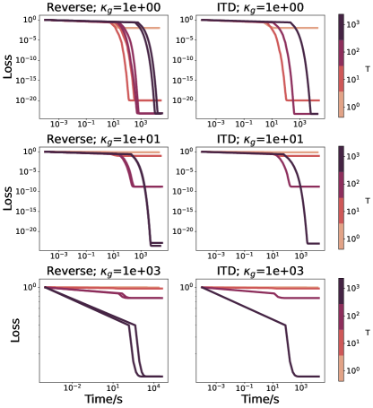
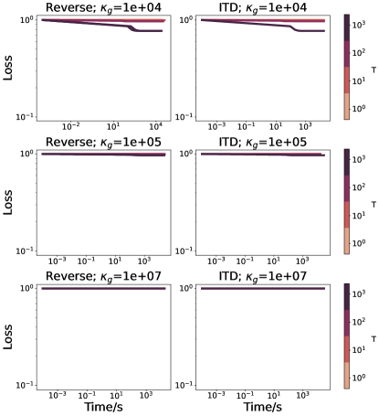
Figure 3: Evolution of the relative error vs. time in seconds for different ITD based methods on the synthetic example. From the left to the right, the first two columns correspond to Reverse and ITD method small conditioning numbers $\kappa_{g}\in\{1,10,10^{3}\}$, last two column are for higher conditioning numbers $\kappa_{g}\in\{10^{4},10^{5},10^{7}\}$. For each method we consider $T\in\{1,10,10^{2},10^{3}\}$. Lightest colors correspond to smaller values of $T$.

F.3 Dataset distillation

Dataset distillation [Wang et al., 2018, Lorraine et al., 2020] consists in learning a small synthetic dataset such that a model trained on this dataset achieves a small error on the training set. Specifically, we consider a classification problem of $C$ classes using a linear model and a training dataset $\mathcal{D}_{tr}$ where each training point $\xi\in\mathcal{D}_{tr}$ is a $d$-dimensional vector with a class $c_{\xi}\in\{1,...,C\}$. The linear model is represented by a matrix $y\in\mathbb{R}^{c\times d}$ multiplying a data point $y\xi$ and providing the logits of each class. The dataset distillation can be cas as a bilevel problem of the form:

$$\min_{x\in\mathbb{R}^{c\times d},\lambda\in\mathbb{R}^{d}} \frac{1}{{\left\lvert\mathcal{D}_{tr}\right\rvert}}\sum_{\xi\in\mathcal{D}_{tr}}CE(y^{\star}(x,\lambda)\xi,c_{\xi}),$$ (275)

$$y^{\star}(x,\lambda)\in\arg\min_{y\in\mathbb{R}^{c\times d}}\frac{1}{C}\sum_{c=1}^{C}CE(yx_{c},c)+\frac{1}{Cd}\sum_{i=1}^{d}\exp(\lambda_{i}){\left\lVert y_{.,i}\right\rVert}^{2}.$$ (276)

where $\lambda\in\mathbb{R}^{d}$ is a vector of hyper-parameter for regularizing the inner-level problem which we found beneficial to add.

Experimental setup. We perform the distillation task on MNIST dataset. We set the step-sizes $\alpha_{k}{=}\beta_{k}{=}0.1$ and $T{=}N{=}10$. We perform a grid-search on the outer-level step-size $\gamma_{k}{\in}\{0.01,0.001,0.0001\}$ and run the algorithms for $k=10000$ iterations.

References

• Ablin etΒ al. [2020] Pierre Ablin, Gabriel PeyrΓ©, and Thomas Moreau. Super-efficiency of automatic differentiation for functions defined as a minimum. In International Conference on Machine Learning, pages 32–41. PMLR, 2020.
• Arjevani etΒ al. [2019] Yossi Arjevani, Yair Carmon, JohnΒ C Duchi, DylanΒ J Foster, Nathan Srebro, and Blake Woodworth. Lower bounds for non-convex stochastic optimization. arXiv preprint arXiv:1912.02365, 2019.
• Baydin etΒ al. [2018] AtilimΒ Gunes Baydin, BarakΒ A Pearlmutter, AlexeyΒ Andreyevich Radul, and JeffreyΒ Mark Siskind. Automatic differentiation in machine learning: a survey. Journal of machine learning research, 18, 2018.
• Bertinetto etΒ al. [2018] Luca Bertinetto, JoaoΒ F Henriques, PhilipΒ HS Torr, and Andrea Vedaldi. Meta-learning with differentiable closed-form solvers. arXiv preprint arXiv:1805.08136, 2018.
• Blondel etΒ al. [2021] Mathieu Blondel, Quentin Berthet, Marco Cuturi, Roy Frostig, Stephan Hoyer, Felipe Llinares-LΓ³pez, Fabian Pedregosa, and Jean-Philippe Vert. Efficient and modular implicit differentiation. arXiv preprint arXiv:2105.15183, 2021.
• Davis and Drusvyatskiy [2018] Damek Davis and Dmitriy Drusvyatskiy. Stochastic subgradient method converges at the rate $o(k^{-1/4})$ on weakly convex functions. arXiv preprint arXiv:1802.02988, 2018.
• Davis etΒ al. [2018] Damek Davis, Dmitriy Drusvyatskiy, KellieΒ J MacPhee, and Courtney Paquette. Subgradient methods for sharp weakly convex functions. Journal of Optimization Theory and Applications, 179(3):962–982, 2018.
• Dempe and Zemkoho [2020] Stephan Dempe and Alain Zemkoho. Bilevel Optimization. Springer, 2020.
• Doan [2020] ThinhΒ T Doan. Nonlinear two-time-scale stochastic approximation: Convergence and finite-time performance. arXiv preprint arXiv:2011.01868, 2020.
• Domke [2012] Justin Domke. Generic methods for optimization-based modeling. In Artificial Intelligence and Statistics, pages 318–326. PMLR, 2012.
• Feurer and Hutter [2019] Matthias Feurer and Frank Hutter. Hyperparameter optimization. In Automated machine learning, pages 3–33. Springer, Cham, 2019.
• Franceschi etΒ al. [2017] Luca Franceschi, Michele Donini, Paolo Frasconi, and Massimiliano Pontil. Forward and reverse gradient-based hyperparameter optimization. In International Conference on Machine Learning, pages 1165–1173. PMLR, 2017.
• Franceschi etΒ al. [2018] Luca Franceschi, Paolo Frasconi, Saverio Salzo, Riccardo Grazzi, and Massimiliano Pontil. Bilevel programming for hyperparameter optimization and meta-learning. In International Conference on Machine Learning, pages 1568–1577. PMLR, 2018.
• Ghadimi and Lan [2012] Saeed Ghadimi and Guanghui Lan. Optimal stochastic approximation algorithms for strongly convex stochastic composite optimization i: A generic algorithmic framework. SIAM Journal on Optimization, 22(4):1469–1492, 2012.
• Ghadimi and Wang [2018] Saeed Ghadimi and Mengdi Wang. Approximation methods for bilevel programming. arXiv preprint arXiv:1802.02246, 2018.
• Gould etΒ al. [2016] Stephen Gould, Basura Fernando, Anoop Cherian, Peter Anderson, RodrigoΒ Santa Cruz, and Edison Guo. On differentiating parameterized argmin and argmax problems with application to bi-level optimization. arXiv preprint arXiv:1607.05447, 2016.
• Grazzi etΒ al. [2020] Riccardo Grazzi, Luca Franceschi, Massimiliano Pontil, and Saverio Salzo. On the iteration complexity of hypergradient computation. In International Conference on Machine Learning, pages 3748–3758. PMLR, 2020.
• Grazzi etΒ al. [2021] Riccardo Grazzi, Massimiliano Pontil, and Saverio Salzo. Convergence properties of stochastic hypergradients. In International Conference on Artificial Intelligence and Statistics, pages 3826–3834. PMLR, 2021.
• Habets [1974] PΒ Habets. Stabilite asyptotique pour des problemes de perturbations singulieres. In Stability Problems, pages 2–18. Springer, 1974.
• Hong etΒ al. [2020a] Mingyi Hong, Hoi-To Wai, Zhaoran Wang, and Zhuoran Yang. A two-timescale framework for bilevel optimization: Complexity analysis and application to actor-critic. arXiv preprint arXiv:2007.05170, 2020a.
• Hong etΒ al. [2020b] Mingyi Hong, Hoi-To Wai, Zhaoran Wang, and Zhuoran Yang. A two-timescale framework for bilevel optimization: Complexity analysis and application to actor-critic. arXiv preprint arXiv:2007.05170, 2020b.
• Ji and Liang [2021] Kaiyi Ji and Yingbin Liang. Lower bounds and accelerated algorithms for bilevel optimization. arXiv preprint arXiv:2102.03926, 2021.
• Ji etΒ al. [2021] Kaiyi Ji, Junjie Yang, and Yingbin Liang. Bilevel optimization: Convergence analysis and enhanced design. In International Conference on Machine Learning, pages 4882–4892. PMLR, 2021.
• Kaledin etΒ al. [2020] Maxim Kaledin, Eric Moulines, Alexey Naumov, Vladislav Tadic, and Hoi-To Wai. Finite time analysis of linear two-timescale stochastic approximation with markovian noise. In Conference on Learning Theory, pages 2144–2203. PMLR, 2020.
• Kingma and Ba [2015] DiederikΒ P. Kingma and Jimmy Ba. Adam: A method for stochastic optimization. In Yoshua Bengio and Yann LeCun, editors, 3rd International Conference on Learning Representations, ICLR 2015, San Diego, CA, USA, May 7-9, 2015, Conference Track Proceedings, 2015.
• Kulunchakov and Mairal [2019] Andrei Kulunchakov and Julien Mairal. Estimate sequences for variance-reduced stochastic composite optimization. In International Conference on Machine Learning, pages 3541–3550. PMLR, 2019.
• Kulunchakov and Mairal [2020] Andrei Kulunchakov and Julien Mairal. Estimate sequences for stochastic composite optimization: Variance reduction, acceleration, and robustness to noise. 2020.
• Lang [2012] Serge Lang. Fundamentals of differential geometry, volume 191. Springer Science & Business Media, 2012.
• Lecouat etΒ al. [2020a] Bruno Lecouat, Jean Ponce, and Julien Mairal. Designing and learning trainable priors with non-cooperative games. arXiv preprint arXiv:2006.14859, 2020a.
• Lecouat etΒ al. [2020b] Bruno Lecouat, Jean Ponce, and Julien Mairal. A flexible framework for designing trainable priors with adaptive smoothing and game encoding. In Conference on Neural Information Processing Systems (NeurIPS), 2020b.
• Liao etΒ al. [2018] Renjie Liao, Yuwen Xiong, Ethan Fetaya, Lisa Zhang, KiJung Yoon, Xaq Pitkow, Raquel Urtasun, and Richard Zemel. Reviving and improving recurrent back-propagation. In International Conference on Machine Learning, pages 3082–3091. PMLR, 2018.
• Lin etΒ al. [2018] Hongzhou Lin, Julien Mairal, and Zaid Harchaoui. Catalyst acceleration for first-order convex optimization: from theory to practice. Journal of Machine Learning Research, 18(1):7854–7907, 2018.
• Liu etΒ al. [2021] Risheng Liu, Jiaxin Gao, Jin Zhang, Deyu Meng, and Zhouchen Lin. Investigating bi-level optimization for learning and vision from a unified perspective: A survey and beyond. arXiv preprint arXiv:2101.11517, 2021.
• Lorraine etΒ al. [2020] Jonathan Lorraine, Paul Vicol, and David Duvenaud. Optimizing millions of hyperparameters by implicit differentiation. In International Conference on Artificial Intelligence and Statistics, pages 1540–1552. PMLR, 2020.
• Mairal etΒ al. [2011] Julien Mairal, Francis Bach, and Jean Ponce. Task-driven dictionary learning. IEEE transactions on pattern analysis and machine intelligence, 34(4):791–804, 2011.
• Nesterov [2003] Yurii Nesterov. Introductory lectures on convex optimization: A basic course, volumeΒ 87. Springer Science & Business Media, 2003.
• Pedregosa [2016] Fabian Pedregosa. Hyperparameter optimization with approximate gradient. In International conference on machine learning, pages 737–746. PMLR, 2016.
• Rajeswaran etΒ al. [2019] Aravind Rajeswaran, Chelsea Finn, ShamΒ M Kakade, and Sergey Levine. Meta-Learning with Implicit Gradients. In H.Β Wallach, H.Β Larochelle, A.Β Beygelzimer, F.Β d\textquotesingle AlchΓ©-Buc, E.Β Fox, and R.Β Garnett, editors, Advances in Neural Information Processing Systems 32 (NeurIPS). Curran Associates, Inc., 2019.
• Saberi and Khalil [1984] Ali Saberi and Hassan Khalil. Quadratic-type lyapunov functions for singularly perturbed systems. IEEE Transactions on Automatic Control, 29(6):542–550, 1984.
• Schmidt etΒ al. [2017] Mark Schmidt, Nicolas LeΒ Roux, and Francis Bach. Minimizing finite sums with the stochastic average gradient. Mathematical Programming, 162(1-2):83–112, 2017.
• Shaban etΒ al. [2019] Amirreza Shaban, Ching-An Cheng, Nathan Hatch, and Byron Boots. Truncated back-propagation for bilevel optimization. In The 22nd International Conference on Artificial Intelligence and Statistics, pages 1723–1732. PMLR, 2019.
• Shewchuk etΒ al. [1994] JonathanΒ Richard Shewchuk etΒ al. An introduction to the conjugate gradient method without the agonizing pain, 1994.
• Stackelberg [1934] H.F.Β Von Stackelberg. MarktformundGleichgewicht. Springer, 1934.
• Wang etΒ al. [2018] Tongzhou Wang, Jun-Yan Zhu, Antonio Torralba, and AlexeiΒ A Efros. Dataset distillation. arXiv preprint arXiv:1811.10959, 2018.
• Yang etΒ al. [2021] Junjie Yang, Kaiyi Ji, and Yingbin Liang. Provably faster algorithms for bilevel optimization. arXiv preprint arXiv:2106.04692, 2021.
• Ye and Ye [1997] JJΒ Ye and XYΒ Ye. Necessary optimality conditions for optimization problems with variational inequality constraints. Mathematics of Operations Research, 22(4):977–997, 1997.
• Ye and Zhu [1995] JJΒ Ye and DLΒ Zhu. Optimality conditions for bilevel programming problems. Optimization, 33(1):9–27, 1995.
• Ye etΒ al. [1997] JJΒ Ye, DLΒ Zhu, and QijiΒ Jim Zhu. Exact penalization and necessary optimality conditions for generalized bilevel programming problems. SIAM Journal on optimization, 7(2):481–507, 1997.