factor-augmented tree ensembles

Abstract

This manuscript proposes to extend the information set of time-series regression trees with latent stationary factors extracted via state-space methods. In doing so, this approach generalises time-series regression trees on two dimensions. First, it allows to handle predictors that exhibit measurement error, non-stationary trends, seasonality and/or irregularities such as missing observations. Second, it gives a transparent way for using domain-specific theory to inform time-series regression trees. Empirically, ensembles of these factor-augmented trees provide a reliable approach for macro-finance problems. This article highlights it focussing on the lead-lag effect between equity volatility and the business cycle in the United States.

factor-augmented tree ensembles

Keywords: Ensemble learning, Factor models, Macro-finance, State-space models.
JEL: C32, C58, E32, E44, G17.

1 Introduction

In time series, the simplicity of regression trees (Morgan and Sonquist, 1963; Breiman et al., 1984; Quinlan, 1986) comes at a cost: irregularities, complicated periodic patterns and non-stationary trends cannot be explicitly modelled, and this is unfortunate given that many real-world examples are subject to them. This is especially true in macroeconomics and finance as shown by a broad body of literature. This includes articles focussed on the output gap, the natural rate of interest and other structural components (Hamilton et al., 2016; Holston et al., 2017; Jarociński and Lenza, 2018; Fries et al., 2018; Del Negro et al., 2019; Barigozzi and Luciani, 2021; Hasenzagl et al., 2022a, b), non-stationary forecasting settings and impulse response functions of economic data in levels (Sims, 1980; Doan et al., 1984; Litterman, 1986; Bańbura et al., 2010; Giannone et al., 2015; Barigozzi et al., 2021), and problems with a prevalence of missing observations comprising nowcasting (Giannone et al., 2008; Bańbura and Modugno, 2014; Cimadomo et al., 2022; Brown et al., 2022).

Following, in spirit, Harvey et al. (1998), this paper proposes to pre-process problematic predictors using state-space representations general enough to deal with all these complexities at once. This operation can be thought as an automated feature engineering process that extracts stationary patterns hidden across multiple predictors, while handling problematic data characteristics. Besides, when the state-space representation is compatible with domain-specific theory, this becomes a transparent way for extracting signals with structural interpretation. The stationary common components recovered from the data, referred hereinbelow as stationary dynamic factors, are then employed as regular predictors for standard time-series regression trees. This manuscript calls them factor-augmented regression trees to stress their dependence on latent components.

For this article, I have built on a broad body of theoretical research on time series. Indeed, factor models originated in psychometrics (Lawley and Maxwell, 1962) as a dimensionality reduction technique. They were later generalised to take into account the autocorrelation structure of time series with the work of Geweke (1977) on dynamic factor models. Over time, these methodologies have been further developed within the state-space literature pioneered by Harvey (1985) to be compatible with data exhibiting peculiar patterns (e.g., non-stationary trends, seasonality) and missing observations. Relevant improvements include the generalized dynamic factor model (Forni et al., 2000; Forni and Lippi, 2001; Forni et al., 2005, 2009), the factor-augmented vector autoregression (Bernanke et al., 2005), quasi maximum likelihood estimation methods (Doz et al., 2012; Barigozzi and Luciani, 2020), the non-stationary dynamic factor model (Barigozzi et al., 2021) and functional analysis extensions (Li et al., 2020).

As for standard regression trees, the factor-augmented version can suffer from over-fitting. Tree ensembles are an efficient way to reduce it without having to use complex vectors of hyperparameters. In order to do that, these methods generally fit a series of regression trees on a range of data subsamples and return aggregate forecasts. This article constructs the ensembles following Breiman (1996). These factor-augmented ensembles are similar to the rotation forest proposed in Rodriguez et al. (2006) and Pardo et al. (2013), but they take into account the autocorrelation structure in the data when estimating the factors and have the higher flexibility embedded in state-space modelling.

Factor-augmented regression trees and their ensembles are also strongly motivated by empirical results in economics and finance. Recent literature on semi-structural models, including Hasenzagl et al. (2022a, b), proposed to enrich statistical trend-cycle decompositions by using a minimal set of economic-driven restrictions. The main advantage of these semi-structural models is that they are able to extract unobserved cyclical and persistent components with economic interpretation, while allowing the data to speak. However, it is often hard to determine reasonable restrictions for most high-dimensional problems. Indeed, in macroeconomics and finance, theory is unclear on the exact dynamics of classical aggregate variables and disaggregated indicators. Also, the literature is not mature enough to understand the precise drivers of new data (e.g., Google searches). Factor-augmented regression trees and their ensembles can be seen as a bridge between the output of small-dimensional semi-structural models (i.e., interpretable cyclical unobserved components) and time series that are not entirely understood from the theoretical standpoint and/or exhibit non-linear dynamics.

As a result, these factor-augmented models are well-suited for tackling macro-finance problems. Indeed, it is often unclear how to model specific drivers and non-linear links between macroeconomic and financial data. For instance, forecasting the yield curve while handling the zero lower bound (Kim and Singleton, 2012; Swanson and Williams, 2014; Bauer and Rudebusch, 2016, 2020), studying exchange rate predictability (Meese and Rogoff, 1983; Engel and West, 2005; Rossi, 2013), or the links between equity and economic aggregates (Nelson, 1976; Fama and Schwert, 1977; Cooper and Priestley, 2009; Campbell and Diebold, 2009). This article focusses on the latter and studies the lead-lag effect between equity volatility and a factor representing the business cycle in the United States. Results show that this is is a strong predictor of equity volatility, especially for small cap stocks. I find this in agreement with a large range of papers such as Gertler and Gilchrist (1994), Sharpe (1994) and Bernanke et al. (1996) whereas it is argued that small firms are more vulnerable to recessions due to the lack of financing options.

2 Methodology

2.1 Regression trees

This subsection describes the population model implied by standard regression trees and their most common estimation method (Breiman et al., 1984).

Assumption 1 (Data).

Let $T\in\mathbb{N}$ and $n\in\mathbb{N}_{0}$. Assume that $Y_{t}$ and $Z_{j,t}$ are finite realisations of some real-valued mean-stationary stochastic processes observed at the time periods $t=1,\ldots,T$ and with $j=1,\ldots,n$.

Assumption 2 (Predictors of standard regression trees).

Let $\boldsymbol{\mathbf{X}}_{t}\vcentcolon=(Y_{t}\;Z_{1,t}\;\ldots\;Z_{n,t})^{\prime}$ be $m\times 1$ dimensional and defined for any point in time $t\in\mathbb{Z}$.

Remark 0.

Throughout the manuscript, the dependency on $n$ and $T$ is highlighted only when strictly necessary to ease the reading experience. Furthermore, specific realisations at some integer point in time $t$ and their general value in the underlying stochastic processes are denoted with the same symbols. However, it should be clear from the context whether the manuscript is referring to the first or second category.

This article describes the regression trees as non-linear forecasting models for $Y_{t}$ based on the information included in $\boldsymbol{\mathbf{X}}_{t-1},\ldots,\boldsymbol{\mathbf{X}}_{t-p}$, for some number of lags $p\in\mathbb{N}$. Without loss of generality, this manuscript focusses on one-step ahead forecasts. Long-run predictions can be generated by computing direct forecasts (Marcellino et al., 2006).

Assumption 3 (Lags).

Let $0<p\ll T-1$.

Assumption 4 (Regression tree model).

In a regression tree setting,

$$Y_{t}=\sum_{i=1}^{|\mathscr{F}|}b_{i}\mathbb{I}\left\{(\boldsymbol{\mathbf{X}}_{t-1}\,\ldots\,\boldsymbol{\mathbf{X}}_{t-p})\in\mathscr{F}_{i}\right\}+\epsilon_{t},$$

whereas $\mathscr{F}$ is an indexed family of disjoint sets of matrices, every $b_{i}$ is a finite constant, $\epsilon_{t}\mathrel{\overset{i.i.d.}{\scalebox{1.5}[1.0]{$\sim$}}}\left(0,\sigma^{2}\right)$ with $\sigma>0$ and finite, for any integer $t$ and $i=1,\ldots,|\mathscr{F}|$. Besides, regression trees assume that

$$\mathbb{E}(Y_{t}|\boldsymbol{\mathbf{X}}_{t-1},\ldots,\boldsymbol{\mathbf{X}}_{t-p},\boldsymbol{\mathbf{b}},\sigma,\mathscr{F})=\sum_{i=1}^{|\mathscr{F}|}b_{i}\mathbb{I}\left\{(\boldsymbol{\mathbf{X}}_{t-1}\,\ldots\,\boldsymbol{\mathbf{X}}_{t-p})\in\mathscr{F}_{i}\right\},$$

for any integer $t$.

Regression trees estimate $\boldsymbol{\mathbf{b}}$, $\sigma$ and $\mathscr{F}$ recursively partitioning the predictor space to find the best fit. There are several modelling choices to take when performing this operation. This article follows common practice by focussing on binary partitions and using the CART algorithm (Breiman et al., 1984). At its first iteration, this estimation method looks for the best possible way to split the predictor space into two regions. This assessment is performed fitting a constant model in each region and minimising the mean square forecast error. Moreover, the splits are computed by inspecting, in turn, each covariate separately. The algorithm iteratively repeats the same operation for each of the resulting regions until some stopping criteria is reached. This manuscript uses DecisionTree.jl to implement it and refers to the estimated parameters with $\boldsymbol{\mathbf{\hat{\theta}}}(\boldsymbol{\mathbf{\gamma}})$ where $\boldsymbol{\mathbf{\gamma}}$ is a vector of hyperparameters.

2.2 Factor-augmented regression trees

This subsection introduces the factor-augmented regression trees: a version of the model in section 2.1 able to handle predictors with irregularities such as structural breaks and missing observations, intricate periodic patterns and non-stationary trends. In order to deal with these complexities, this subsection introduces a series of changes to the model and estimation algorithm.

Factor-augmented regression trees allow for these complexities in the data redefining $\boldsymbol{\mathbf{Z}}_{t}$ and $\boldsymbol{\mathbf{X}}_{t}$ as detailed in assumptions 5 to 7.

Assumption 5 (State-space representation: data).

Assume that $Z_{i,t}$ is finite realisations of some real-valued stochastic process observed at the time periods in the set $\mathscr{T}_{i}\subseteq\{t:t\in\mathbb{Z},\,1\leq t\leq T\}$ for every $i=1,\ldots,n$.

Assumption 6 (State-space representation: structure).

Let $\boldsymbol{\mathbf{Z}}_{t}$ be a $n\times 1$ real random vector that allows the state-space representation

$$Z_{i,t} =g_{i,t}(\boldsymbol{\mathbf{\Phi}}_{t},\xi_{i,t}),$$

$$\boldsymbol{\mathbf{\Phi}}_{t} =\boldsymbol{\mathbf{h}}_{t}(\boldsymbol{\mathbf{\Phi}}_{t-1},\boldsymbol{\mathbf{\zeta}}_{t}),$$

where $g_{i,t}$ and $\boldsymbol{\mathbf{h}}_{t}$ are continuous and differentiable functions, $\boldsymbol{\mathbf{\Phi}}_{t}$ denotes a vector of $q>0$ latent states, $\boldsymbol{\mathbf{\xi}}_{t}\mathrel{\overset{i.i.d.}{\scalebox{1.5}[1.0]{$\sim$}}}(\boldsymbol{\mathbf{0}}_{n\times 1},\boldsymbol{\mathbf{R}}_{t})$ and $\boldsymbol{\mathbf{\zeta}}_{t}\mathrel{\overset{i.i.d.}{\scalebox{1.5}[1.0]{$\sim$}}}(\boldsymbol{\mathbf{0}}_{q\times 1},\boldsymbol{\mathbf{Q}}_{t})$, for any integer $t$ and $i=1,\ldots,n$. Also, it is assumed that every $\boldsymbol{\mathbf{\Phi}}_{t}$ includes a $\bar{q}\times 1$ vector of stationary common factors $\boldsymbol{\mathbf{\phi}}_{t}$, with $0<\bar{q}\ll n$ and $q\geq\bar{q}$. Since the observations start from the time period $t=1$, it is further assumed that $\boldsymbol{\mathbf{\Phi}}_{1}=\boldsymbol{\mathbf{h}}_{0}(\boldsymbol{\mathbf{\zeta}}_{0})$. This allows the evaluation of the state-space representation with the observed data.

Remark 0 (Non-stationarity).

Differently than with assumptions 1 to 2, assumption 5 does not assume that the underlying stochastic process is stationary. As a result, assumption 6 is compatible with non-stationary trends and co-integrated relationships.

Assumption 7 (Predictors of factor-augmented trees).

Factor-augmented regression trees include the stationary common factors in the predictors (as is, transformed in a way that does not alter data ordering and preserves stationarity, or both). Formally, this is achieved including these common components in the predictor matrix $\boldsymbol{\mathbf{X}}_{t}$ jointly with $Y_{t}$ and updating $m$ accordingly.

Remark 0 (Information set).

Factor-augmented regression trees extend the information set of a tree autoregression for $Y_{t}$ with stationary common factors, while discarding idiosyncratic noise in the predictors and non-stationary trends, and handling data irregularities. The simplest case is when the predictor matrix is extended to include these stationary factors as they come out from the state-space. Formally, this is achieved by letting $\boldsymbol{\mathbf{X}}_{t}\vcentcolon=(Y_{t}\,\;\boldsymbol{\mathbf{\phi}}_{t})$ be a $m\times 1$ vector of time series, with $m\vcentcolon=1+\bar{q}$.

The structure of the model is exactly as described in section 2.1, but uses the newly defined predictor matrix and value for $m$. However, the estimation process is different and structured as a two-step method. In the first step, the state space in assumption 6 is estimated with any algorithm compatible with the data complexities described above, including, but not limited to, the EM (Dempster et al., 1977; Rubin and Thayer, 1982; Shumway and Stoffer, 1982; Watson and Engle, 1983; Bańbura and Modugno, 2014; Barigozzi and Luciani, 2020), ECM (Meng and Rubin, 1993; Pellegrino, 2023) and ECME algorithms (Liu and Rubin, 1994). In the second and final step, the predictor matrix is formed on the basis of the estimated states and the regression tree is trained with CART.

It is worth stressing that the main difference between factor-augmented regression trees and the individual base learners of rotation forests (Rodriguez et al., 2006; Pardo et al., 2013) lies in the technique used for reducing the dimensionality of the data. Instead of using Principal Component Analysis, factor-augmented regression tree models use a state-space. In doing so, this approach explicitly models the temporal factors dynamics, permits to pinpoint specific unobserved components and allows for data that exhibits peculiar patterns such as non-stationary trends. Note that factor-augmented regression trees could be extended to use selected idiosyncratic periodic patterns as additional predictors. This could be done by redefining $\boldsymbol{\mathbf{\phi}}$ into a vector of “selected cycles”, both common and idiosyncratic. However, this would increase the computational burden and, without limitations, the risk of generating spurious splits.

2.3 Tree ensembles

Tree ensembles are methods that combine multiple regression trees, in order to produce more efficient predictions than the individual base learners (i.e., the trees themselves).

For simplicity of illustration, this article focusses on ensemble averaging and, in particular, on bootstrap aggregating or bagging (Breiman, 1996). This method obtains the increase in efficiency estimating a large number of regression trees on random data subsamples and combining their predictions taking a sample average. Intuitively, this reduces over-fitting since the base learners are not trained on the original data, but on random subsamples generated from it. The more heterogeneous and numerous the subsamples the better in terms of efficiency. This can be formalised following an approach equivalent to Hastie et al. (2009, section 15.2).

This article follows common practice and uses the bootstrap version proposed in Efron and Gong (1983, section 7) to generate the subsamples. This approach considers each covariate-response pair as a single datapoint and constructs data subsamples via independent bootstrap (Efron, 1979a, b, 1981). In other words, it resamples covariate-response pairs from the original data to generate the subsamples. In particular, in the case of the factor-augmented trees this is done focussing on the factor-response pairs.

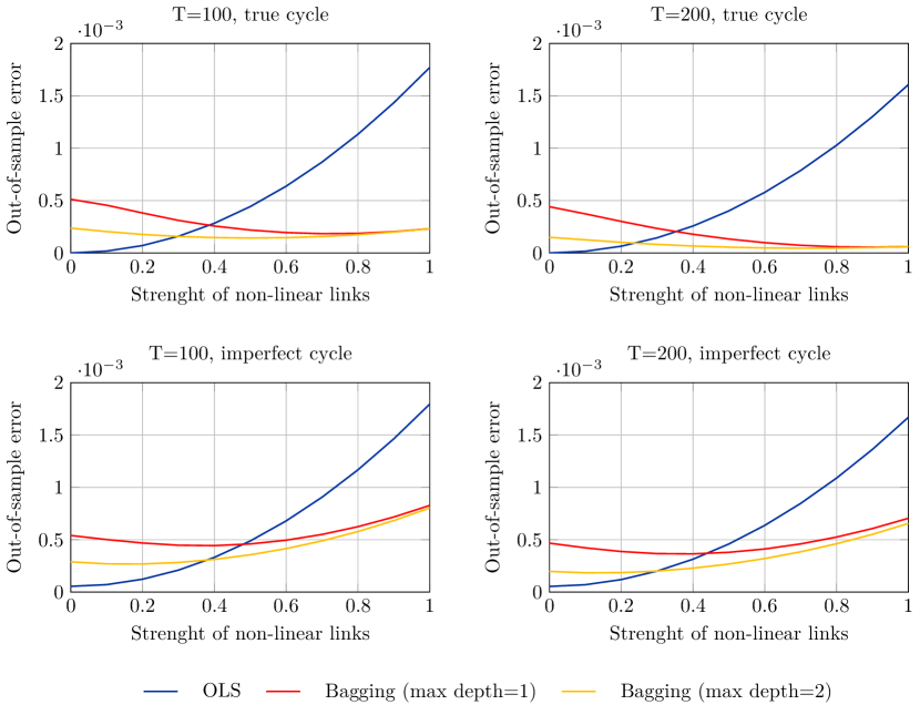
Figure 1: Simulation results.

3 Monte Carlo study

Before delving into the empirical analysis, these factor-augmented ensembles are examined through the lens of the following Monte Carlo study.

I simulate data from

$$Y_{t}=w\left(\rho_{1}\,\mathbb{I}\left\{\phi_{t-1}\leq 0\right\}+\rho_{2}\,\mathbb{I}\left\{\phi_{t-1}>0\right\}\right)+(1-w)\,\rho_{3}\,\phi_{t-1},$$

$$\phi_{t}=c_{1}\,\phi_{t-1}+c_{2}\phi_{t-2}+\zeta_{t},$$

where $0\leq w\leq 1$. The dynamics of the stationary cycle $\phi_{t}$ are set as in Clark (1987, Table 1) to simulate a component similar to the US business cycle. The coefficients linking the simulated target to the stationary cycle are such that $\rho_{1}\mathrel{\overset{i.i.d.}{\scalebox{1.5}[1.0]{$\sim$}}}U(-0.1,0)$ and $\rho_{2}\mathrel{\overset{i.i.d.}{\scalebox{1.5}[1.0]{$\sim$}}}U(0,0.1)$. For simplicity, $\rho_{3}=1$. The model allows for non-linear links between the target and cycle. These non-linearities are controlled by the scalar $w$. The constraint $\rho_{1}\leq\rho_{2}$ simulates data resembling procyclical asset returns that react differently to recessions than expansions.

I generate the model $1,000$ times for $w=0,0.1,\ldots,1$ and $T=100,200$. For each replicate, I use the first half of the sample to regress the target onto the cycle and predict the remaining target data points out-of-sample. The regressions are performed both via OLS (as in standard factor regressions) and bagging (as in the factor-based ensembles proposed herein). Figure 1 shows the out-of-sample mean squared error for all models, aggregated over the 1,000 simulations. The first row reports the results for the case in which the estimation and forecasts are based on the true cycle. The second row shows the equivalent results for the case in which the cycle is contaminated with random noise drawn from a normal distribution with the same variance as the cycle innovations themselves. The results indicate that traditional factor regressions are subpar, except when the data generating process is strongly linear. In fact, even with minor non-linearities, bagging produces more accurate out-of-sample predictions. More broadly, this suggests that factor-augmented ensembles are likely to outperform traditional approaches based on linear models when predicting data with suspected non-linearities.

Table 1: Monthly macro-financial indicators. The macroeconomic data is sampled from January 1984 to December 2020 and downloaded in a real-time fashion from the Archival Federal Reserve Economic Data (ALFRED) database. The financial indicators are sampled from January 1984 to January 2021 and downloaded from the Federal Reserve Economic Data (FRED) database. Table 3 provides a glossary for the acronyms.

Mnemonic	Description	Transformation	Source
TCU	Capacity utilization: total index	Levels	FRB
INDPRO	Industrial production: total index	Levels	FRB
RPCE	Real personal consumption expendit.	Levels	BEA
PAYEMS	Total nonfarm employment	Levels	BLS
EMRATIO	Employment-population ratio	Levels	BLS
UNRATE	Unemployment rate	Levels	BLS
WTISPLC	Spot crude oil price (WTI)	YoY returns	FRBSL
CPIAUCNS	CPI: all items	YoY returns	BLS
CPILFENS	CPI: all items excl. food and energy	YoY returns	BLS
WILL5000IND	Wilshire 5000 TMI	MoM returns (squared)	WA
WILLLRGCAP	Wilshire US Large-Cap TMI	MoM returns (squared)	WA
WILLLRGCAPVAL	Wilshire US Large-Cap Value TMI	MoM returns (squared)	WA
WILLLRGCAPGR	Wilshire US Large-Cap Growth TMI	MoM returns (squared)	WA
WILLMIDCAP	Wilshire US Mid-Cap TMI	MoM returns (squared)	WA
WILLMIDCAPVAL	Wilshire US Mid-Cap Value TMI	MoM returns (squared)	WA
WILLMIDCAPGR	Wilshire US Mid-Cap Growth TMI	MoM returns (squared)	WA
WILLSMLCAP	Wilshire US Small-Cap TMI	MoM returns (squared)	WA
WILLSMLCAPVAL	Wilshire US Small-Cap Value TMI	MoM returns (squared)	WA
WILLSMLCAPGR	Wilshire US Small-Cap Growth TMI	MoM returns (squared)	WA

4 Advantages for empirical macro-finance

Academic insights indicate that financial returns are linked to macroeconomic fundamentals. However, these relations are usually hard to find and may be subject to non-linearities.

In principle, a simple way to exploit this behaviour would be running a non-linear predictive regressions using the lagged business cycle as predictor and some function of a financial return of interest as a response. However, this is easier said than done. Indeed, the business cycle itself is an unobserved variable that reflects the cyclical co-movement between a series of non-stationary economic indicators (e.g., output, unemployment and inflation). Besides, the non-linear links with the financial returns have an unclear form and, thus, it is hard to model them in a parametric way.

Factor-augmented regression trees and their ensembles represent a simple approach to the problem, compatible with its complexities. In fact, the state-space in assumption 6 can be thought as a way for extracting the business cycle from a set of predictors and the regression tree as a model that does not require an a-priori parametrisation of the non-linear link between macroeconomic and financial data.

4.1 Empirical setting

This subsection illustrates the advantages of factor-augmented ensembles focussing on the United States. Specifically, it employs these techniques for predicting equity volatility – measured as squared returns – of the financial indices in table 1 as a function of lagged information on themselves and the business cycle.

In order to estimate the state of the economy in real time, this section uses a state-space representation similar, in spirit, to the one proposed in Hasenzagl et al. (2022a, b). This modelling choice implies that each macroeconomic indicator in table 1 is considered as the sum of non-stationary trends and causal cycles, one of which can be interpreted as the US business cycle. The trends account for the persistence in the data and provide a view on a series of structural components such as the natural rate of unemployment and trend inflation. By linking together key variables such as the real personal consumption expenditures, unemployment rate and inflation through the business cycle, the model is compatible with economic relationships such as the Phillips curve and the Okun’s law (interpreting consumption as a proxy for GDP). A complex lag structure in the coefficients associated with the business cycle allows to take into account frictions in the economy (for instance, in the labour market). Finally, the idiosyncratic cycles account for autocorrelation in the error terms (if any).

This approach can be formalised as follows.

Assumption 8 (State-space representation: trend-cycle model).

For any integer $t$, let $\boldsymbol{\mathbf{Z}}_{t}$ denote the macroeconomic indicators included in the first block of table 1. For simplicity, assume that the data in $\boldsymbol{\mathbf{Z}}_{t}$ is the order reported in the table and standardised such that each $i$-th series is divided for a given scaling factor $\eta_{i}$, for $i=1,\ldots,n$ with $n=9$. Hence, let

$$\left(\begin{array}[]{c}Z_{1,t}\\ Z_{2,t}\\ Z_{3,t}\\ Z_{4,t}\\ Z_{5,t}\\ Z_{6,t}\\ Z_{7,t}\\ Z_{8,t}\\ Z_{9,t}\end{array}\right) =\left(\begin{array}[]{c}\tau_{1,t}\\ \tau_{2,t}\\ \tau_{3,t}\\ \tau_{4,t}\\ \tau_{5,t}\\ \tau_{6,t}\\ \tau_{7,t}\\ \frac{\tau_{8,t}}{\eta_{8}}\\ \frac{\tau_{8,t}}{\eta_{9}}\end{array}\right)+\left(\begin{array}[]{cccc}1\\ \Upsilon_{1,1}+\Upsilon_{1,2}L+\ldots+\Upsilon_{1,p}L^{p-1}\\ \Upsilon_{2,1}+\Upsilon_{2,2}L+\ldots+\Upsilon_{2,p}L^{p-1}\\ \Upsilon_{3,1}+\Upsilon_{3,2}L+\ldots+\Upsilon_{3,p}L^{p-1}\\ \Upsilon_{4,1}+\Upsilon_{4,2}L+\ldots+\Upsilon_{4,p}L^{p-1}\\ \Upsilon_{5,1}+\Upsilon_{5,2}L+\ldots+\Upsilon_{5,p}L^{p-1}\\ \Upsilon_{6,1}+\Upsilon_{6,2}L+\ldots+\Upsilon_{6,p}L^{p-1}\\ \Upsilon_{7,1}+\Upsilon_{7,2}L+\ldots+\Upsilon_{7,p}L^{p-1}\\ \Upsilon_{8,1}+\Upsilon_{8,2}L+\ldots+\Upsilon_{8,p}L^{p-1}\end{array}\right)\psi_{1,t}+\left(\begin{array}[]{c}\psi_{2,t}\\ \psi_{3,t}\\ \psi_{4,t}\\ \psi_{5,t}\\ \psi_{6,t}\\ \psi_{7,t}\\ \psi_{8,t}\\ \psi_{9,t}\\ \psi_{10,t}\end{array}\right)+\boldsymbol{\mathbf{\xi}}_{t}$$

where $\psi_{1,t}$ is a causal AR($p$) denoting the business cycle; $\tau_{1,t},\ldots,\tau_{8,t}$ are second-order smooth trends (Kitagawa and Gersch, 1996, section 8.1); headline and core inflation share a common trend (the so-called trend inflation); $\psi_{2,t},\ldots,\psi_{10,t}$ are causal AR(1) idiosyncratic noises; $\boldsymbol{\mathbf{\xi}}_{t}\mathrel{\overset{w.n.}{\scalebox{1.5}[1.0]{$\sim$}}}N\left(\boldsymbol{\mathbf{0}}_{9\times 1},\varepsilon\cdot\boldsymbol{\mathbf{I}}_{9}\right)$ for a small positive $\varepsilon$, similarly to Bańbura and Modugno (2014). Going forward, the number of lags $p$ is set to $12$ months in order to allow for a relatively large memory in the business cycle. The dynamics for the states and estimation method for this trend-cycle model are further detailed in appendix A.

Remark 0 (Trend inflation).

Post estimation, the standardisation is removed to use the original units. In doing so, the scaling factors associated with trend inflation are also removed. Hence, headline and core inflation have the same trend once the standardisation is lifted.

The factor-augmented ensembles extend the information set of traditional autoregression trees including with the estimated business cycle. The latter is used both in levels and with a selected range of transformations. Formally, in order to compute a prediction referring to a generic time $t+1$, the factor-augmented ensembles use a vector of predictors containing the target values referring to time $t,\ldots,t-11$ and the augmentation

$$\begin{pmatrix}\hat{\psi}_{1,t+11|t}\\ \vdots\\ \hat{\psi}_{1,t-11|t}\\ \hline\cr\hat{\psi}_{1,t+11|t}-\hat{\psi}_{1,t+10|t}\\ \vdots\\ \hat{\psi}_{1,t-10|t}-\hat{\psi}_{1,t-11|t}\\ \hline\cr\hat{\psi}_{1,t+11|t}-\hat{\psi}_{1,t|t}\\ \vdots\\ \hat{\psi}_{1,t+2|t}-\hat{\psi}_{1,t|t}\\ \hline\cr\hat{\psi}_{1,t|t}-\hat{\psi}_{1,t-2|t}\\ \vdots\\ \hat{\psi}_{1,t|t}-\hat{\psi}_{1,t-11|t}\end{pmatrix},$$ (1)

where $\hat{\psi}_{1,t+j|t}$ denotes the estimate of the business cycle for a generic period $t+j$ computed with the information set available at time $t$. While the first block in the factor augmentation gives a direct view on the business cycle levels, the following ones are useful for computing splits directly on its turning points and making a better use of the data.

Each ensemble is regulated via a vector of hyperparameters that includes those specifics to the state-space estimation and the minimum number of observations per leaf. These tuning parameters are determined on a sample going from January 1984 to the end of January 2005. The ALFRED data vintage used for structuring the macroeconomic selection sample includes the information was available right before the end of January 2005. Since this article uses a two-step method, hyperparameters are selected first for the trend-cycle model and then for the factor-augmented ensembles. The trend-cycle model is tuned as illustrated in section A.5. Next, the minimum number of observations per leaf of each ensemble is determined with a pseudo out-of-sample criterion and a grid search on the equally spaced $\mathscr{H}_{RT}\vcentcolon=\{0.01,10,15,\ldots,0.5\}$ with $|\mathscr{H}_{RT}|=25$. The minimum number of observations per leaf is expressed in percentage terms with respect to the number of time periods available. Both steps use the first half of the selection sample for the estimation and the second half to validate the results.

4.2 In-sample results

This subsection presents key in-sample findings to aid understanding each stage involved in constructing these factor-augmented ensembles

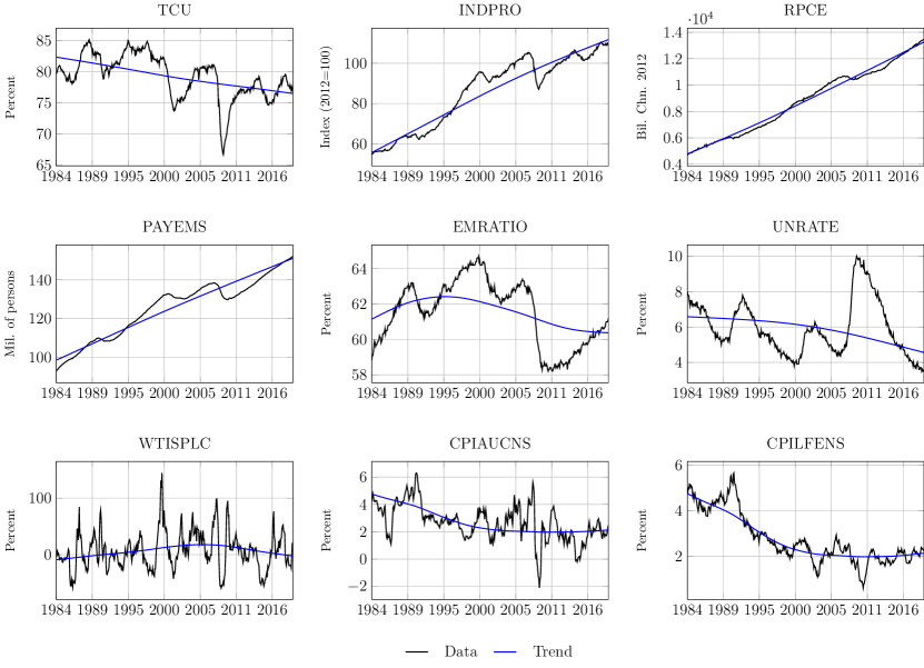
Figure 2: Trends estimated with the full-sample available on the 28th February 2020.

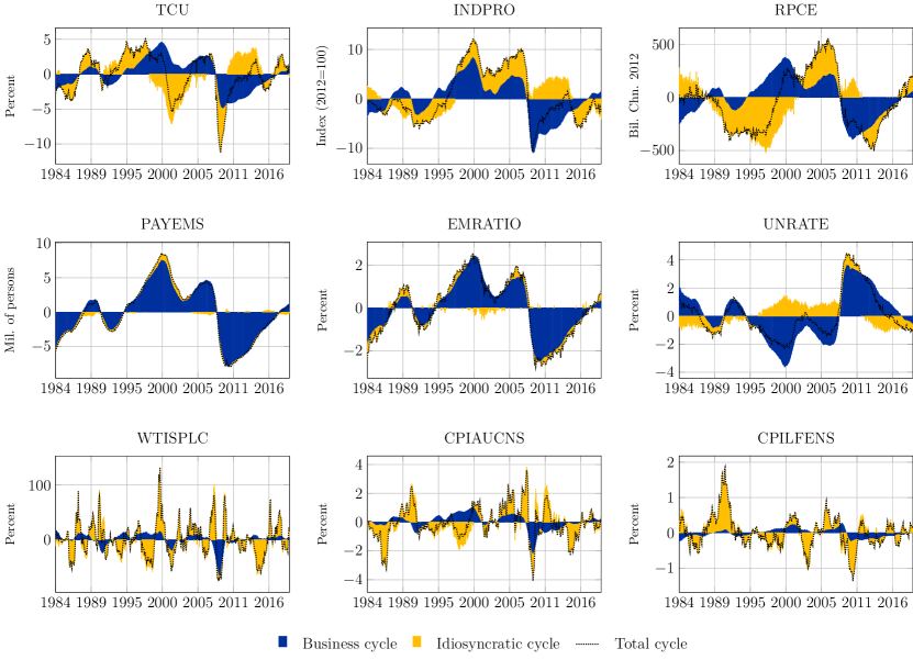
Figure 3: Cycles decomposition estimated with the full-sample available on the 28th February 2020.

In the first step, the model extracts persistent and transitory components from macroeconomic data. Figures 2 to 3 shows an in-sample snapshot of the economy captured by this trend-cycle decomposition based on monthly data from January 1984 to February 2020. This is the full sample available on the 28th February 2020 as it was recorded on the ALFRED database. In other words, the last pre COVID-19 vintage for the macroeconomic data in this analysis. Figure 2 compares the data in levels with the estimated trends, while figure 3 decomposes the cycles into common and idiosyncratic fluctuations. The results are compatible with papers including Hasenzagl et al. (2022a, b) and Barigozzi and Luciani (2021), and show that, while there is a strong heterogeneity across macroeconomic indicators, the business cycle explains most of the cyclical fluctuations. Besides, these findings also show that the business cycle is synchronised with the NBER dating, which means that expansions (contractions) in this latent component are usually associated with economic growth (recessions).

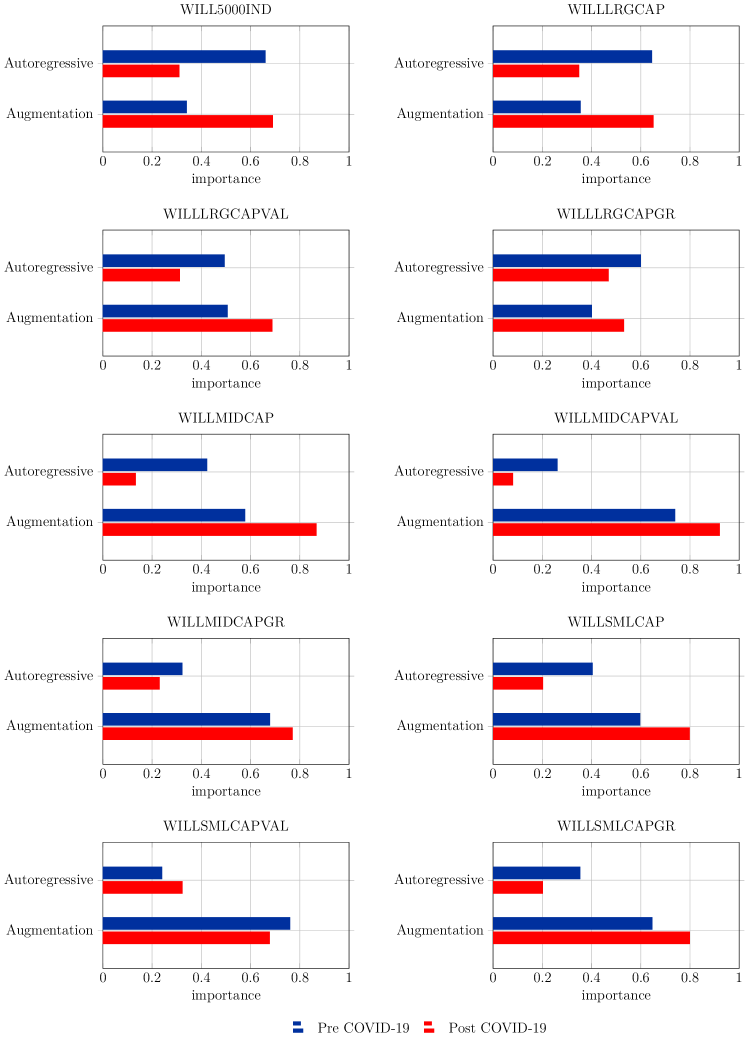
Figure 4: Importance weights pre and post COVID-19. The “Autoregressive” and “Augmentation” bars reflect the cumulative weights for the lagged target and transformed business cycle. Pre COVID-19 weights are computed using the ALFRED data vintage for the 28th February 2020 and corresponding Wilshire data.

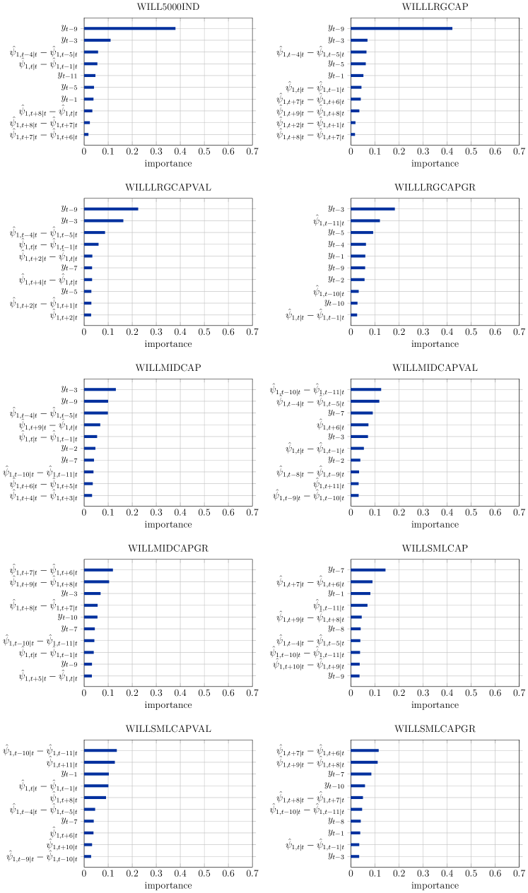
Figure 5: Importance weights pre COVID-19: top 10 predictors. Pre COVID-19 weights are computed using the macroeconomic series available on the 28th February 2020 on ALFRED and the corresponding Wilshire data.

The second step builds on the trend-cycle decomposition and uses the business cycle – both in levels and transformed as in equation 1 – to extend the information set of tree ensembles for equity volatility. One of the advantages of tree-based models with respect to alternative machine learning techniques is that they are highly interpretable and allow to inspect the predictability drivers. Figure 4 and the additional figures in appendix B compare the factor-augmented ensembles estimated pre and post COVID-19 (i.e., estimating it first with data as at 28th February 2020 and then with the latest vintage available) by looking at the bagging importance weights: the number of times, in percentage points, that a predictor is selected to create a split in the underlying factor-augmented regression trees which is, essentially, an internal ranking. Figure 4 reports the total importance of the lagged target and factor augmentation. Mid to small cap shares are usually more vulnerable than blue chips to changes in economic conditions. Indeed, a broad range of papers such as Gertler and Gilchrist (1994), Sharpe (1994) and Bernanke et al. (1996) argue that small firms do not have a broad range of financing options and mostly use intermediaries to access credit. This leaves them more at risk during a downturn when banks become more selective with respect to credit extensions. Therefore, it is not surprising that the factor augmentation is especially crucial for the Wilshire indices referring to these market capitalisations. In addition, figure 4 highlights how the factor augmentation is even more relevant post COVID-19, a period of unprecedented high volatility and uncertainty. Figures 5 to 6 highlight a high heterogeneity across targets.

4.3 Real-time evaluation

Influential studies (e.g., Orphanides and Norden, 2002) have warned about the potential risks of utilising cyclical latent variables of economic significance, such as the business cycle or the output gap, without ensuring that the associated forecasting benefits are robust. As a result, this subsection assesses the real-time predictability of these factor-augmented tree ensembles both pre and post COVID-19.

I have started this analysis supposing to be right before the end of January 2005, the moment in time when the hyperparameters were calibrated (cf. section 4.1). Based on the information available at that time, I estimated the ensembles, in turn, for each target and produced the corresponding one-step-ahead forecasts. Subsequently, I performed out-of-sample testing by re-estimating the models and generating fresh predictions every time a new ALFRED vintage became available. The macroeconomic test sample comprises 861 vintages, each with a minimum of 2277 observations, and, in adherence to the aforementioned guidelines, the evaluation does not look forward in the future.

Table 2: Mean squared errors associated to bagging forecasts, relative to those for naive predictions constant at zero. Values lower than 1 denote cases where this naive benchmark was outperformed by bootstrap aggregating. The mean squared errors are computed using a one-month ahead forecast horizon, in real-time, over the target observations spanning from February 2005 to January 2021. The columns marked as “Autoregressive” refer to ensembles whose information set includes lags of the target variable only. The columns marked as “Augmented” denote the factor-augmented ensembles in section 4. The Pre COVID-19 period uses the ALFRED vintages up to the 28th February 2020 release (included) and corresponding Wilshire data.

Target	Pre COVID-19			Post COVID-19
	Autoregressive	Augmented		Autoregressive	Augmented
WILL5000IND	0.760	0.739		0.754	0.739
WILLLRGCAP	0.768	0.745		0.756	0.738
WILLLRGCAPVAL	0.770	0.765		0.779	0.773
WILLLRGCAPGR	0.765	0.702		0.729	0.689
WILLMIDCAP	0.783	0.758		0.815	0.803
WILLMIDCAPVAL	0.784	0.763		0.863	0.859
WILLMIDCAPGR	0.835	0.720		0.799	0.732
WILLSMLCAP	0.750	0.704		0.788	0.767
WILLSMLCAPVAL	0.757	0.755		0.816	0.823
WILLSMLCAPGR	1.132	0.683		1.007	0.713

Table 2 provides a summary of the out-of-sample findings, showing the mean squared error associated with the bagging forecasts relative to the one for a naive benchmark constant at zero. In other words an metrics that, when lower than one, indicates the ensembles are more accurate than this simple model. Besides, table 2 compares standard autoregressive ensembles (i.e., without the factor-augmentation) with those that leverage on the business cycle and its transformation. These figures reveal two crucial findings. First, the factor-augmented models are more accurate than classic bagging for all targets and especially for the volatility of mid to small cap stocks, in accordance with section 4.2. Second, almost all ensembles outperform the corresponding naive benchmark, which may appear obvious initially, but not necessarily so for linear forecasting models such as those detailed in table 4. Hence, this provides further confirmation of the superiority of bootstrap aggregating.

5 Concluding remarks

Most econometric techniques rely on simplifying assumptions that are typically based on highly stylised theoretical models. While these assumptions enable researchers to obtain easily interpretable estimates, it is challenging to justify their use for complex real-world problems, which are frequently characterised by non-linear relationships with unclear parametric forms – this is especially true when modelling the joint dynamics between macroeconomic and financial data. Conversely, machine learning techniques are unconstrained by the nature of the problem, but heavily reliant on observable data and often difficult to interpret. This manuscript proposes to bridge the gap between these families of techniques by developing a hybrid between structural time series (Harvey, 1985, 1990) and machine learning. More specifically, the manuscript presents an approach where indicators with unclear or complex dynamics are connected to latent states of economic interest using tree ensembles (Breiman, 1996, 2001). This is a two-stage method since these latent variables are estimated separately and before the ensembles via state-space models informed by domain-specific theory.

From a methodological perspective, this is advantageous for two reasons. First, it generalises tree-based regressions to allow for predictors with non-stationary trends, seasonality, peculiar cyclical patterns and missing values. Second, this approach permits to inform ensembles with domain-specific theory extending their information set using latent variables with structural interpretation. Empirically, this is of particular relevance for macro-finance. Indeed, it is relatively straightforward to link returns and other financial variables of interest with unobserved components representing economic concepts such as the output gap. This article describes in greater detail the lead-lag effect between equity volatility and the US business cycle and finds that the current economic conditions are strong predictors of equity volatility when allowing for non-linearities. This is studied both in-sample and out-of-sample, and results are particularly strong for stocks with small market capitalisation. The latter is in agreement with the broad body of literature including Gertler and Gilchrist (1994), Sharpe (1994) and Bernanke et al. (1996) that find similar firms more vulnerable to downturns due to a lack of financing options.

Factor-augmented ensembles could also be beneficial for related empirical problems such as the study of links between foreign exchange rates and fundamentals (Meese and Rogoff, 1983; Engel and West, 2005; Rossi, 2013). Similar problems are left open for future research.

Notes

1. 1 Bayesian techniques surveyed, for instance, in Särkkä (2013) can also be used. In that case, $\boldsymbol{\mathbf{\phi}}_{t}$ would be a point estimate (e.g., mean or median) of the stationary dynamic factors distribution at time $t$.
2. 2 This is fundamentally the same difference between traditional and dynamic factor models (see, for example, Barigozzi and Luciani, 2020, for a comparison between these approaches).
3. 3 In this empirical example, $\varepsilon=10^{-4}$.
4. 4 This difference in the selection method is determined by the higher computational complexity required to estimate and forecast with factor-augmented tree ensembles.
5. 5 This numerical approximation is governed by $\varepsilon$ in assumption 8.
6. 6 The weights in Pellegrino [2023] are set to be equal to zero for all variables with the exception of headline inflation which has weight equal to one.

Appendix A Business cycle estimation

A.1 Trend-cycle model

Re-write the model in assumption 8 in the state-space form

$$\boldsymbol{\mathbf{Z}}_{t} =\boldsymbol{\mathbf{B}}\boldsymbol{\mathbf{\Phi}}_{t}+\boldsymbol{\mathbf{\xi}}_{t},$$

$$\boldsymbol{\mathbf{\Phi}}_{t} =\boldsymbol{\mathbf{C}}\boldsymbol{\mathbf{\Phi}}_{t-1}+\boldsymbol{\mathbf{D}}\boldsymbol{\mathbf{\zeta}}_{t}.$$

The innovation in the transition equation $\boldsymbol{\mathbf{\zeta}}_{t}\mathrel{\overset{w.n}{\scalebox{1.5}[1.0]{$\sim$}}}N\left(\boldsymbol{\mathbf{0}}_{r\times 1},\boldsymbol{\mathbf{\Sigma}}\right)$ with $\boldsymbol{\mathbf{\Sigma}}$ being a $r\times r$ positive definite real diagonal matrix and $r=18$. The transition matrices are sparse and the non-zero entries are such that

$$\boldsymbol{\mathbf{C}}\vcentcolon=\left(\begin{array}[]{ccc | ccc | ccc | ccccc}1&\cdot&\cdot&1&\cdot&\cdot&\cdot&\cdot&\cdot&\cdot&\cdot&\cdot&\cdot&\cdot\\ \cdot&\ddots&\cdot&\cdot&\ddots&\cdot&\cdot&\cdot&\cdot&\cdot&\cdot&\cdot&\cdot&\cdot\\ \cdot&\cdot&1&\cdot&\cdot&1&\cdot&\cdot&\cdot&\cdot&\cdot&\cdot&\cdot&\cdot\\ \hline\cr\cdot&\cdot&\cdot&1&\cdot&\cdot&\cdot&\cdot&\cdot&\cdot&\cdot&\cdot&\cdot&\cdot\\ \cdot&\cdot&\cdot&\cdot&\ddots&\cdot&\cdot&\cdot&\cdot&\cdot&\cdot&\cdot&\cdot&\cdot\\ \cdot&\cdot&\cdot&\cdot&\cdot&1&\cdot&\cdot&\cdot&\cdot&\cdot&\cdot&\cdot&\cdot\\ \hline\cr\cdot&\cdot&\cdot&\cdot&\cdot&\cdot&\pi_{1}&\cdot&\cdot&\cdot&\cdot&\cdot&\cdot&\cdot\\ \cdot&\cdot&\cdot&\cdot&\cdot&\cdot&\cdot&\ddots&\cdot&\cdot&\cdot&\cdot&\cdot&\cdot\\ \cdot&\cdot&\cdot&\cdot&\cdot&\cdot&\cdot&\cdot&\pi_{n}&\cdot&\cdot&\cdot&\cdot&\cdot\\ \hline\cr\cdot&\cdot&\cdot&\cdot&\cdot&\cdot&\cdot&\cdot&\cdot&\pi_{n+1}&\pi_{n+2}&\ldots&\pi_{n+p-1}&\pi_{n+p}\\ \cdot&\cdot&\cdot&\cdot&\cdot&\cdot&\cdot&\cdot&\cdot&1&\cdot&\ldots&\cdot&\cdot\\ \cdot&\cdot&\cdot&\cdot&\cdot&\cdot&\cdot&\cdot&\cdot&\cdot&1&\ddots&\vdots&\vdots\\ \cdot&\cdot&\cdot&\cdot&\cdot&\cdot&\cdot&\cdot&\cdot&\vdots&\ddots&\ddots&\vdots&\vdots\\ \cdot&\cdot&\cdot&\cdot&\cdot&\cdot&\cdot&\cdot&\cdot&\cdot&\ldots&\ldots&1&\cdot\\ \end{array}\right),$$

$$\hskip 27.9001pt\begin{array}[]{ccccccc ccc cccc ccccc}\lx@intercol\hfil\underbrace{\hskip 20.25003pt}_{q\times 8}\hfil\lx@intercol&\lx@intercol\hfil\underbrace{\hskip 23.40009pt}_{q\times 8}\hfil\lx@intercol&\lx@intercol\hfil\underbrace{\hskip 32.4001pt}_{q\times 9}\hfil\lx@intercol&\lx@intercol\hfil\underbrace{\hskip 99.00017pt}_{q\times p}\hfil\lx@intercol\end{array}$$

$$\boldsymbol{\mathbf{D}}\vcentcolon=\left(\begin{array}[]{ccc | ccc | ccc}\cdot&\cdot&\cdot&\cdot&\cdot&\cdot&\cdot\\ \cdot&\cdot&\cdot&\cdot&\cdot&\cdot&\cdot\\ \cdot&\cdot&\cdot&\cdot&\cdot&\cdot&\cdot\\ \hline\cr 1&\cdot&\cdot&\cdot&\cdot&\cdot&\cdot\\ \cdot&\ddots&\cdot&\cdot&\cdot&\cdot&\cdot\\ \cdot&\cdot&1&\cdot&\cdot&\cdot&\cdot\\ \hline\cr\cdot&\cdot&\cdot&1&\cdot&\cdot&\cdot\\ \cdot&\cdot&\cdot&\cdot&\ddots&\cdot&\cdot\\ \cdot&\cdot&\cdot&\cdot&\cdot&1&\cdot\\ \hline\cr\cdot&\cdot&\cdot&\cdot&\cdot&\cdot&1\\ \cdot&\cdot&\cdot&\cdot&\cdot&\cdot&\cdot\end{array}\right),$$

$$\hskip 27.9001pt\begin{array}[]{ccc ccc ccc}\lx@intercol\hfil\underbrace{\hskip 20.25003pt}_{q\times 8}\hfil\lx@intercol&\lx@intercol\hfil\underbrace{\hskip 20.25003pt}_{q\times 9}\hfil\lx@intercol&\lx@intercol\hfil\underbrace{\hskip 0.90005pt}_{q\times 1}\hfil\lx@intercol\end{array}$$

where $\boldsymbol{\mathbf{\pi}}$ is a $n+p\times 1$ vector of finite real parameters and $q=25+p$. The measurement coefficient matrix is also sparse and the non-zero entries are such that

$$\boldsymbol{\mathbf{B}}\vcentcolon=\left(\begin{array}[]{cccccccc | ccc | ccccccccc | cccc }1&\cdot&\cdot&\cdot&\cdot&\cdot&\cdot&\cdot&\cdot&\ldots&\cdot&1&\cdot&\cdot&\cdot&\cdot&\cdot&\cdot&\cdot&\cdot&1&\cdot&\ldots&\cdot\\ \cdot&1&\cdot&\cdot&\cdot&\cdot&\cdot&\cdot&\cdot&\ldots&\cdot&\cdot&1&\cdot&\cdot&\cdot&\cdot&\cdot&\cdot&\cdot&\tilde{\Upsilon}_{1,1}&\tilde{\Upsilon}_{1,2}&\ldots&\tilde{\Upsilon}_{1,p}\\ \cdot&\cdot&1&\cdot&\cdot&\cdot&\cdot&\cdot&\cdot&\ldots&\cdot&\cdot&\cdot&1&\cdot&\cdot&\cdot&\cdot&\cdot&\cdot&\tilde{\Upsilon}_{2,1}&\tilde{\Upsilon}_{2,2}&\ldots&\tilde{\Upsilon}_{2,p}\\ \cdot&\cdot&\cdot&1&\cdot&\cdot&\cdot&\cdot&\cdot&\ldots&\cdot&\cdot&\cdot&\cdot&1&\cdot&\cdot&\cdot&\cdot&\cdot&\tilde{\Upsilon}_{3,1}&\tilde{\Upsilon}_{3,2}&\ldots&\tilde{\Upsilon}_{3,p}\\ \cdot&\cdot&\cdot&\cdot&1&\cdot&\cdot&\cdot&\cdot&\ldots&\cdot&\cdot&\cdot&\cdot&\cdot&1&\cdot&\cdot&\cdot&\cdot&\tilde{\Upsilon}_{4,1}&\tilde{\Upsilon}_{4,2}&\ldots&\tilde{\Upsilon}_{4,p}\\ \cdot&\cdot&\cdot&\cdot&\cdot&1&\cdot&\cdot&\cdot&\ldots&\cdot&\cdot&\cdot&\cdot&\cdot&\cdot&1&\cdot&\cdot&\cdot&\tilde{\Upsilon}_{5,1}&\tilde{\Upsilon}_{5,2}&\ldots&\tilde{\Upsilon}_{5,p}\\ \cdot&\cdot&\cdot&\cdot&\cdot&\cdot&1&\cdot&\cdot&\ldots&\cdot&\cdot&\cdot&\cdot&\cdot&\cdot&\cdot&1&\cdot&\cdot&\tilde{\Upsilon}_{6,1}&\tilde{\Upsilon}_{6,2}&\ldots&\tilde{\Upsilon}_{6,p}\\ \cdot&\cdot&\cdot&\cdot&\cdot&\cdot&\cdot&\frac{1}{\eta_{8}}&\cdot&\ldots&\cdot&\cdot&\cdot&\cdot&\cdot&\cdot&\cdot&\cdot&1&\cdot&\tilde{\Upsilon}_{7,1}&\tilde{\Upsilon}_{7,2}&\ldots&\tilde{\Upsilon}_{7,p}\\ \cdot&\cdot&\cdot&\cdot&\cdot&\cdot&\cdot&\frac{1}{\eta_{9}}&\cdot&\ldots&\cdot&\cdot&\cdot&\cdot&\cdot&\cdot&\cdot&\cdot&\cdot&1&\tilde{\Upsilon}_{8,1}&\tilde{\Upsilon}_{8,2}&\ldots&\tilde{\Upsilon}_{8,p}\end{array}\right),$$

$$\hskip 27.9001pt\begin{array}[]{cccccccc ccc ccccccccc cccc}\lx@intercol\hfil\underbrace{\hskip 51.30005pt}_{9\times 8}\hfil\lx@intercol&\lx@intercol\hfil\underbrace{\hskip 19.34998pt}_{9\times 8}\hfil\lx@intercol&\lx@intercol\hfil\underbrace{\hskip 55.80006pt}_{9\times 9}\hfil\lx@intercol&\lx@intercol\hfil\underbrace{\hskip 63.90016pt}_{9\times p}\hfil\lx@intercol\end{array}$$

where $\boldsymbol{\mathbf{\tilde{\Upsilon}}}$ is a $8\times p$ matrix of finite real parameters and $\tilde{\Upsilon}_{i,j}\approx\Upsilon_{i,j}$, for any $i=1,\ldots,8$ and $j=1,\ldots,p$. This representation implies that

$$\boldsymbol{\mathbf{\Phi}}_{t}\vcentcolon=\left(\begin{array}[]{ccc | ccc | cccc | cccc}\tau_{1,t}&\ldots&\tau_{8,t}&\delta_{1,t}&\ldots&\delta_{8,t}&\psi_{2,t}&\psi_{3,t}&\ldots&\psi_{10,t}&\psi_{1,t}&\psi_{1,t-1}&\ldots&\psi_{1,t-p+1}\end{array}\right)^{\prime}.$$

$$\hskip 27.9001pt\begin{array}[]{ccc ccc cccc cccc}\lx@intercol\hfil\underbrace{\hskip 37.35pt}_{8\times 1}\hfil\lx@intercol&\lx@intercol\hfil\underbrace{\hskip 38.70009pt}_{8\times 1}\hfil\lx@intercol&\lx@intercol\hfil\underbrace{\hskip 61.65015pt}_{9\times 1}\hfil\lx@intercol&\lx@intercol\hfil\underbrace{\hskip 85.50014pt}_{p\times 1}\hfil\lx@intercol\end{array}$$

The initial conditions for the states are such that $\boldsymbol{\mathbf{\Phi}}_{0}\mathrel{\overset{w.n.}{\scalebox{1.5}[1.0]{$\sim$}}}N(\boldsymbol{\mathbf{\mu}}_{0},\boldsymbol{\mathbf{\Omega}}_{0})$, where $\boldsymbol{\mathbf{\mu}}_{0}$ and $\boldsymbol{\mathbf{\Omega}}_{0}$ denote a $q\times 1$ real vector and a $q\times q$ positive definite real covariance matrix. The matrix $\boldsymbol{\mathbf{\Omega}}_{0}$ is sparse and the entries that can differ from zero are those with coordinates $(i,j)\in\{(i,j):i=j\text{ and }1\leq i\leq 25\}\cup\{(i,j):25<i\leq q\text{ and }25<j\leq q\}$.

Remark 0.

The empirical application assumes that $\boldsymbol{\mathbf{\Sigma}}$ is diagonal. This implies an exact factor model (i.e., no cross-sectional dependence in the idiosyncratic components) and, in doing so, it simplifies the narrative. However, this assumption may be too restrictive for more general problems. For similar problems, the assumptions could be relaxed and the ECM algorithm described in this appendix could be presented as a penalised quasi maximum likelihood estimation method building on the theoretical results in Barigozzi and Luciani [2020].

A.2 The Expectation-Conditional Maximisation algorithm

Denote the model free parameters with

$$\boldsymbol{\mathbf{\vartheta}}\vcentcolon=\left(\begin{array}[]{cccccccc}\boldsymbol{\mathbf{\mu}}_{0}^{\prime}&\text{vech}(\boldsymbol{\mathbf{\Omega}}_{0})^{\prime}&\text{vec}(\boldsymbol{\mathbf{\tilde{\Upsilon}}})^{\prime}&\boldsymbol{\mathbf{\pi}}^{\prime}&\Sigma_{1,1}&\Sigma_{2,2}&\ldots&\Sigma_{r,r}\end{array}\right)^{\prime}.$$

The ECM algorithm estimates these coefficients by repeating the optimisation process illustrated in definition 1 until convergence.

Definition 1 (ECM estimation routine).

At any $k+1>1$ iteration, the ECM algorithm computes the vector of coefficients

$$\boldsymbol{\mathbf{\hat{\vartheta}}}_{s}^{k+1}(\boldsymbol{\mathbf{\gamma}})\vcentcolon=\operatorname*{arg\,max}_{\underline{\boldsymbol{\mathbf{\vartheta}}}\,\in\,\mathscr{R}}\,\mathbb{E}\left[\mathcal{L}(\underline{\boldsymbol{\mathbf{\vartheta}}}\,|\,\boldsymbol{\mathbf{Z}}_{1:s},\boldsymbol{\mathbf{\Phi}}_{1:s})\,|\,\mathscr{Z}(s),\,\boldsymbol{\mathbf{\hat{\vartheta}}}_{s}^{k}(\boldsymbol{\mathbf{\gamma}})\right]-\mathbb{E}\left[\mathcal{P}(\underline{\boldsymbol{\mathbf{\vartheta}}},\boldsymbol{\mathbf{\gamma}})\,|\,\mathscr{Z}(s),\,\boldsymbol{\mathbf{\hat{\vartheta}}}_{s}^{k}(\boldsymbol{\mathbf{\gamma}})\right],$$

where $\mathscr{R}$ denotes the region in which the AR cycles (common and idiosyncratic) are causal, $\mathscr{Z}(s)$ is the information set available at time $s$,

$$\mathcal{L}(\underline{\boldsymbol{\mathbf{\vartheta}}}\,|\,\boldsymbol{\mathbf{Z}}_{1:s},\boldsymbol{\mathbf{\Phi}}_{1:s})\simeq -\frac{1}{2}\ln|\underline{\boldsymbol{\mathbf{\Omega}}_{0}}|-\frac{1}{2}\operatorname{Tr}\Big{[}\underline{\boldsymbol{\mathbf{\Omega}}_{0}}^{-1}(\boldsymbol{\mathbf{\Phi}}_{0}-\underline{\boldsymbol{\mathbf{\mu}}_{0}})(\boldsymbol{\mathbf{\Phi}}_{0}-\underline{\boldsymbol{\mathbf{\mu}}_{0}})^{\prime}\Big{]}$$ (2)

$$-\frac{s}{2}\ln|\underline{\boldsymbol{\mathbf{\Sigma}}}|-\frac{1}{2}\operatorname{Tr}\Big{[}\sum_{t=1}^{s}\underline{\boldsymbol{\mathbf{\Sigma}}}^{-1}(\boldsymbol{\mathbf{\Phi}}_{*,t}-\underline{\boldsymbol{\mathbf{C}}}_{\,*}\boldsymbol{\mathbf{\Phi}}_{t-1})(\boldsymbol{\mathbf{\Phi}}_{*,t}-\underline{\boldsymbol{\mathbf{C}}}_{\,*}\boldsymbol{\mathbf{\Phi}}_{t-1})^{\prime}\Big{]}$$

$$-\frac{s}{2}\ln|\underline{\boldsymbol{\mathbf{R}}}|-\frac{1}{2}\operatorname{Tr}\Big{[}\sum_{t=1}^{s}\underline{\boldsymbol{\mathbf{R}}}^{-1}(\boldsymbol{\mathbf{Z}}_{t}-\underline{\boldsymbol{\mathbf{B}}}\boldsymbol{\mathbf{\Phi}}_{t})(\boldsymbol{\mathbf{Z}}_{t}-\underline{\boldsymbol{\mathbf{B}}}\boldsymbol{\mathbf{\Phi}}_{t})^{\prime}\Big{]},$$

$\boldsymbol{\mathbf{\Phi}}_{*,t}\equiv\underline{\boldsymbol{\mathbf{D}}}^{\prime}\boldsymbol{\mathbf{\Phi}}_{t}$, $\underline{\boldsymbol{\mathbf{C}}}_{\,*}\equiv\underline{\boldsymbol{\mathbf{D}}}^{\prime}\underline{\boldsymbol{\mathbf{C}}}$, and the underlined matrices denote the state-space coefficients implied by $\underline{\boldsymbol{\mathbf{\vartheta}}}$. Besides,

$$\mathcal{P}(\underline{\boldsymbol{\mathbf{\vartheta}}},\boldsymbol{\mathbf{\gamma}})\vcentcolon=+\frac{1-\alpha}{2} \left(\big{\|}\underline{\boldsymbol{\mathbf{\pi}}}_{\,1:n}\,\boldsymbol{\mathbf{\Gamma}}(\boldsymbol{\mathbf{\gamma}},1)^{\frac{1}{2}}\big{\|}_{\text{F}}^{2}+\big{\|}\underline{\boldsymbol{\mathbf{\pi}}}_{\,n+1:n+p}^{\prime}\,\boldsymbol{\mathbf{\Gamma}}(\boldsymbol{\mathbf{\gamma}},1)^{\frac{1}{2}}\big{\|}_{\text{F}}^{2}+\big{\|}\underline{\boldsymbol{\mathbf{\tilde{\Upsilon}}}}\,\boldsymbol{\mathbf{\Gamma}}(\boldsymbol{\mathbf{\gamma}},p)^{\frac{1}{2}}\big{\|}_{\text{F}}^{2}\right)$$

$$+\frac{\alpha}{2} \left(\big{\|}\underline{\boldsymbol{\mathbf{\pi}}}_{\,1:n}\,\boldsymbol{\mathbf{\Gamma}}(\boldsymbol{\mathbf{\gamma}},1)\big{\|}_{1,1}+\big{\|}\underline{\boldsymbol{\mathbf{\pi}}}_{\,n+1:n+p}^{\prime}\,\boldsymbol{\mathbf{\Gamma}}(\boldsymbol{\mathbf{\gamma}},1)\big{\|}_{1,1}+\big{\|}\underline{\boldsymbol{\mathbf{\tilde{\Upsilon}}}}\,\boldsymbol{\mathbf{\Gamma}}(\boldsymbol{\mathbf{\gamma}},p)\big{\|}_{1,1}\right)$$

where, for any $l\in\mathbb{N}$,

$$\boldsymbol{\mathbf{\Gamma}}(\boldsymbol{\mathbf{\gamma}},l)\vcentcolon=\lambda\begin{pmatrix}1&0&\ldots&0\\ 0&\beta&\ldots&0\\ \vdots&\ddots&\ddots&\vdots\\ 0&\ldots&\ldots&\beta^{l-1}\end{pmatrix},$$

$\lambda\geq 0$, $0\leq\alpha\leq 1$ and $\beta\geq 1$ are hyperparameters included in $\boldsymbol{\mathbf{\gamma}}$. The state-space coefficients for the first iteration are initialised as in section A.3.

Remark 0 (Objective functions).

The function in equation 2 is the so-called complete-data (i.e., fully observed data and known latent states) log-likelihood, while $\mathcal{P}(\underline{\boldsymbol{\mathbf{\vartheta}}},\boldsymbol{\mathbf{\gamma}})$ represents the generalised elastic-net penalty used in Pellegrino [2023].

Remark 0 (Underlined coefficients).

Some of the underlined state-space coefficients are partially or fully fixed in accordance with the structure in section A.1. For instance, $\boldsymbol{\mathbf{D}}=\underline{\boldsymbol{\mathbf{D}}}$ since $\boldsymbol{\mathbf{D}}$ does not contain free parameters.

Assumption 9 (Convergence).

The ECM algorithm is said to be converged when the criteria in algorithm 1 are met.

The optimisation in definition 1 is performed in two steps. The first one (E-step) involves the computation of the expectations in equation 2. The second step (CM-step) conditionally maximises the resulting expected penalised log-likelihood with respect to the free parameters.

It is convenient to write down the E-step on the basis of the output of a Kalman smoother compatible with incomplete time series, as in Shumway and Stoffer [1982] and Watson and Engle [1983]. The required output is introduced in definition 2 and used in proposition 1 to compute the expected log-likelihood.

Definition 2 (Kalman smoother output).

The hereinbefore mentioned Kalman smoother output is

$$\boldsymbol{\mathbf{\hat{\Phi}}}_{t}\vcentcolon=\mathbb{E}\,\Big{[}\boldsymbol{\mathbf{\Phi}}_{t}\,|\,\mathscr{Z}(s),\boldsymbol{\mathbf{\hat{\vartheta}}}_{s}^{k}(\boldsymbol{\mathbf{\gamma}})\Big{]},$$

$$\boldsymbol{\mathbf{\hat{P}}}_{t,t-j}\vcentcolon=\text{Cov}\,\Big{[}\boldsymbol{\mathbf{\Phi}}_{t},\boldsymbol{\mathbf{\Phi}}_{t-j}\,|\,\mathscr{Z}(s),\boldsymbol{\mathbf{\hat{\vartheta}}}_{s}^{k}(\boldsymbol{\mathbf{\gamma}})\Big{]},$$

for any $k\geq 0$, $0\leq j\leq t$ and $t\geq 0$. Let also $\boldsymbol{\mathbf{\hat{P}}}_{t}\equiv\boldsymbol{\mathbf{\hat{P}}}_{t,t}$.

Remark 0.

These estimates are computed as in Pellegrino [2023].

Furthermore, definition 3 is useful to formalise which measurements are observed at every single point in time.

Definition 3 (Observed measurements).

Let

$$\mathscr{T}\vcentcolon=\bigcup_{i=1}^{n}\mathscr{T}_{i},$$

$$\mathscr{T}(s)\vcentcolon=\{t:t\in\mathscr{T},\,1\leq t\leq s\},$$

describe two sets representing the points in time (either over the full sample or up to time $s$) in which we observe at least one measurement, for $1\leq s\leq T$. Let also

$$\mathscr{V}_{t}\vcentcolon=\{i:t\in\mathscr{T}_{i},\,1\leq i\leq n\},$$

for $1\leq t\leq T$. Thus, let

$$\boldsymbol{\mathbf{Z}}_{t}^{obs}\vcentcolon=\big{(}Z_{i,t}\big{)}_{i\in\mathscr{V}_{t}}$$

$$\boldsymbol{\mathbf{B}}_{t}^{obs}\vcentcolon=\boldsymbol{\mathbf{A}}_{t}\boldsymbol{\mathbf{B}}$$

be the vector of observed measurements at time $t$ and the corresponding $|\mathscr{V}_{t}|\times q$ matrix of coefficients, for any $t\in\mathscr{T}$. Every $\boldsymbol{\mathbf{A}}_{t}$ is indeed a selection matrix constituted by ones and zeros that permits to retrieve the appropriate rows of $\boldsymbol{\mathbf{B}}$ for every $t\in\mathscr{T}$.

Proposition 1.

Let

$$\mathcal{L}_{e}\left[\underline{\boldsymbol{\mathbf{\vartheta}}}\,|\,\mathscr{Z}(s),\boldsymbol{\mathbf{\hat{\vartheta}}}_{s}^{k}(\boldsymbol{\mathbf{\gamma}})\right]\equiv\mathbb{E}\left[\mathcal{L}(\underline{\boldsymbol{\mathbf{\vartheta}}}\,|\,\boldsymbol{\mathbf{Z}}_{1:s},\boldsymbol{\mathbf{\Phi}}_{1:s})\,|\,\mathscr{Z}(s),\boldsymbol{\mathbf{\hat{\vartheta}}}_{s}^{k}(\boldsymbol{\mathbf{\gamma}})\right].$$

Building on definition 2, it follows that

$$\mathcal{L}_{e}\left[\underline{\boldsymbol{\mathbf{\vartheta}}}\,|\,\mathscr{Z}(s),\boldsymbol{\mathbf{\hat{\vartheta}}}_{s}^{k}(\boldsymbol{\mathbf{\gamma}})\right]\simeq -\frac{1}{2}\ln|\underline{\boldsymbol{\mathbf{\Omega}}_{0}}|-\frac{1}{2}\operatorname{Tr}\Big{[}\underline{\boldsymbol{\mathbf{\Omega}}_{0}}^{-1}(\boldsymbol{\mathbf{\hat{E}}}-\boldsymbol{\mathbf{\hat{\Phi}}}_{0}\underline{\boldsymbol{\mathbf{\mu}}_{0}}^{\prime}-\underline{\boldsymbol{\mathbf{\mu}}_{0}}\boldsymbol{\mathbf{\hat{\Phi}}}_{0}^{\prime}+\underline{\boldsymbol{\mathbf{\mu}}_{0}}\,\underline{\boldsymbol{\mathbf{\mu}}_{0}}^{\prime})\Big{]}$$

$$-\frac{s}{2}\ln|\underline{\boldsymbol{\mathbf{\Sigma}}}|-\frac{1}{2}\operatorname{Tr}\Big{[}\underline{\boldsymbol{\mathbf{\Sigma}}}^{-1}(\boldsymbol{\mathbf{\hat{F}}}_{s}-\boldsymbol{\mathbf{\hat{G}}}_{s}\underline{\boldsymbol{\mathbf{C}}}_{\,*}^{\prime}-\underline{\boldsymbol{\mathbf{C}}}_{\,*}\boldsymbol{\mathbf{\hat{G}}}_{s}^{\prime}+\underline{\boldsymbol{\mathbf{C}}}_{\,*}\boldsymbol{\mathbf{\hat{H}}}_{s}\underline{\boldsymbol{\mathbf{C}}}_{\,*}^{\prime})\Big{]}$$

$$-\frac{1}{2\varepsilon}\operatorname{Tr}\left\{\sum_{t\in\mathscr{T}(s)}\left[\left(\boldsymbol{\mathbf{Z}}_{t}^{obs}-\underline{\boldsymbol{\mathbf{B}}}_{\,t}^{obs}\,\boldsymbol{\mathbf{\hat{\Phi}}}_{t}\right)\left(\boldsymbol{\mathbf{Z}}_{t}^{obs}-\underline{\boldsymbol{\mathbf{B}}}_{\,t}^{obs}\,\boldsymbol{\mathbf{\hat{\Phi}}}_{t}\right)^{\prime}+\underline{\boldsymbol{\mathbf{B}}}_{\,t}^{obs}\,\boldsymbol{\mathbf{\hat{P}}}_{t}\,\underline{\boldsymbol{\mathbf{B}}}_{\,t}^{{obs}^{\prime}}\right]\right\},$$

where

$$\boldsymbol{\mathbf{\hat{E}}}\vcentcolon=\mathbb{E}\Big{[}\boldsymbol{\mathbf{\Phi}}_{0}\boldsymbol{\mathbf{\Phi}}_{0}^{\prime}\,|\,\mathscr{Z}(s),\boldsymbol{\mathbf{\hat{\vartheta}}}_{s}^{k}(\boldsymbol{\mathbf{\gamma}})\Big{]}=\boldsymbol{\mathbf{\hat{\Phi}}}_{0}\boldsymbol{\mathbf{\hat{\Phi}}}_{0}^{\prime}+\boldsymbol{\mathbf{\hat{P}}}_{0},$$

$$\boldsymbol{\mathbf{\hat{F}}}_{s}\vcentcolon=\sum_{t=1}^{s}\mathbb{E}\Big{[}\boldsymbol{\mathbf{\Phi}}_{*,t}\boldsymbol{\mathbf{\Phi}}_{*,t}^{\prime}\,|\,\mathscr{Z}(s),\boldsymbol{\mathbf{\hat{\vartheta}}}_{s}^{k}(\boldsymbol{\mathbf{\gamma}})\Big{]}=\sum_{t=1}^{s}\underline{\boldsymbol{\mathbf{D}}}^{\prime}\left(\boldsymbol{\mathbf{\hat{\Phi}}}_{t}\boldsymbol{\mathbf{\hat{\Phi}}}_{t}^{\prime}+\boldsymbol{\mathbf{\hat{P}}}_{t}\right)\underline{\boldsymbol{\mathbf{D}}},$$

$$\boldsymbol{\mathbf{\hat{G}}}_{s}\vcentcolon=\sum_{t=1}^{s}\mathbb{E}\Big{[}\boldsymbol{\mathbf{\Phi}}_{*,t}\boldsymbol{\mathbf{\Phi}}_{t-1}^{\prime}\,|\,\mathscr{Z}(s),\boldsymbol{\mathbf{\hat{\vartheta}}}_{s}^{k}(\boldsymbol{\mathbf{\gamma}})\Big{]}=\sum_{t=1}^{s}\underline{\boldsymbol{\mathbf{D}}}^{\prime}\left(\boldsymbol{\mathbf{\hat{\Phi}}}_{t}\boldsymbol{\mathbf{\hat{\Phi}}}_{t-1}^{\prime}+\boldsymbol{\mathbf{\hat{P}}}_{t,t-1}\right),$$

$$\boldsymbol{\mathbf{\hat{H}}}_{s}\vcentcolon=\sum_{t=1}^{s}\mathbb{E}\Big{[}\boldsymbol{\mathbf{\Phi}}_{t-1}\boldsymbol{\mathbf{\Phi}}_{t-1}^{\prime}\,|\,\mathscr{Z}(s),\boldsymbol{\mathbf{\hat{\vartheta}}}_{s}^{k}(\boldsymbol{\mathbf{\gamma}})\Big{]}=\sum_{t=1}^{s}\left(\boldsymbol{\mathbf{\hat{\Phi}}}_{t-1}\boldsymbol{\mathbf{\hat{\Phi}}}_{t-1}^{\prime}+\boldsymbol{\mathbf{\hat{P}}}_{t-1}\right).$$

Proof.

The proof is analogous to the one in Pellegrino [2023, Proposition 4]. ∎

Remark 0.

$\boldsymbol{\mathbf{D}}=\underline{\boldsymbol{\mathbf{D}}}$ plays the role of a selection matrix. In particular premultiplying by $\underline{\boldsymbol{\mathbf{D}}}^{\prime}$ allows to select rows and postmultiplying by $\underline{\boldsymbol{\mathbf{D}}}$ columns.

Lemma 1.

The conditional expectation for the penalty in definition 1 is

$$\mathbb{E}\left[\mathcal{P}(\underline{\boldsymbol{\mathbf{\vartheta}}},\boldsymbol{\mathbf{\gamma}})\,|\,\mathscr{Z}(s),\boldsymbol{\mathbf{\hat{\vartheta}}}_{s}^{k}(\boldsymbol{\mathbf{\gamma}})\right]=\mathcal{P}(\underline{\boldsymbol{\mathbf{\vartheta}}},\boldsymbol{\mathbf{\gamma}}).$$

Proof.

A formal proof is not reported since it is immediate. Indeed, the penalty function in this ECM algorithm depends only on the current vector of coefficients and hyperparameters. ∎

The CM-step conditionally maximises the expected penalised log-likelihood

$$\mathcal{M}_{e}\left[\underline{\boldsymbol{\mathbf{\vartheta}}},\boldsymbol{\mathbf{\gamma}}\,|\,\mathscr{Z}(s),\boldsymbol{\mathbf{\hat{\vartheta}}}_{s}^{k}(\boldsymbol{\mathbf{\gamma}})\right]\vcentcolon=\mathcal{L}_{e}\left[\underline{\boldsymbol{\mathbf{\vartheta}}}\,|\,\mathscr{Z}(s),\boldsymbol{\mathbf{\hat{\vartheta}}}_{s}^{k}(\boldsymbol{\mathbf{\gamma}})\right]-\mathcal{P}(\underline{\boldsymbol{\mathbf{\vartheta}}},\boldsymbol{\mathbf{\gamma}})$$ (3)

to estimate the state-space parameters. The estimated coefficients are denoted with an “hat” symbol. Besides, an $s$ subscript is used for highlighting the sample size and a superscript for denoting the ECM iteration.

Lemma 2.

The ECM estimator at a generic iteration $k+1>0$ for $\boldsymbol{\mathbf{\mu}}_{0}$ is

$$\boldsymbol{\mathbf{\hat{\mu}}}_{0,s}^{k+1}(\boldsymbol{\mathbf{\gamma}})=\boldsymbol{\mathbf{\hat{\Phi}}}_{0}$$

and the estimator for $\boldsymbol{\mathbf{\Omega}}_{0}$ is a sparse covariance matrix whose non-zero entries are

$$\Big{[}\boldsymbol{\mathbf{\hat{\Omega}}}_{0,s}^{k+1}(\boldsymbol{\mathbf{\gamma}})\Big{]}_{i,j}=\Big{[}\boldsymbol{\mathbf{\hat{P}}}_{0}\Big{]}_{i,j},$$

for $(i,j)\in\{(i,j):i=j\text{ and }1\leq i\leq 25\}\cup\{(i,j):25<i\leq q\text{ and }25<j\leq q\}$.

Proof.

The derivative of equation 3 with respect to $\underline{\boldsymbol{\mathbf{\mu}}_{0}}$ is

$$\frac{\partial\mathcal{M}_{e}\left[\underline{\boldsymbol{\mathbf{\vartheta}}},\boldsymbol{\mathbf{\gamma}}\,|\,\mathscr{Z}(s),\boldsymbol{\mathbf{\hat{\vartheta}}}_{s}^{k}(\boldsymbol{\mathbf{\gamma}})\right]}{\partial\underline{\boldsymbol{\mathbf{\mu}}_{0}}}=-\frac{1}{2}\underline{\boldsymbol{\mathbf{\Omega}}_{0}}^{-1}\left(-2\boldsymbol{\mathbf{\hat{\Phi}}}_{0}+2\underline{\boldsymbol{\mathbf{\mu}}_{0}}\right).$$

It follows that the maximiser for the expected penalised log-likelihood is

$$\boldsymbol{\mathbf{\hat{\mu}}}_{0,s}^{k+1}(\boldsymbol{\mathbf{\gamma}})=\boldsymbol{\mathbf{\hat{\Phi}}}_{0}.$$

The derivative of equation 3 with respect to $\underline{\boldsymbol{\mathbf{\Omega}}_{0}}$ and fixing $\underline{\boldsymbol{\mathbf{\mu}}_{0}}=\boldsymbol{\mathbf{\hat{\mu}}}_{0,s}^{k+1}(\boldsymbol{\mathbf{\gamma}})$ is

$$-\frac{1}{2}\underline{\boldsymbol{\mathbf{\Omega}}_{0}}^{-1}+\frac{1}{2}\underline{\boldsymbol{\mathbf{\Omega}}_{0}}^{-1}\left[\boldsymbol{\mathbf{\hat{E}}}-\boldsymbol{\mathbf{\hat{\Phi}}}_{0}\boldsymbol{\mathbf{\hat{\Phi}}}_{0}^{\prime}\right]\underline{\boldsymbol{\mathbf{\Omega}}_{0}}^{-1}=-\frac{1}{2}\underline{\boldsymbol{\mathbf{\Omega}}_{0}}^{-1}+\frac{1}{2}\underline{\boldsymbol{\mathbf{\Omega}}_{0}}^{-1}\boldsymbol{\mathbf{\hat{P}}}_{0}\,\underline{\boldsymbol{\mathbf{\Omega}}_{0}}^{-1}.$$

as also shown in Pellegrino [2023]. Given the assumptions in section A.1 on the structure of $\boldsymbol{\mathbf{\Omega}}_{0}$, it follows that $\boldsymbol{\mathbf{\hat{\Omega}}}_{0,s}^{k+1}(\boldsymbol{\mathbf{\gamma}})$ is a sparse matrix whose non-zero entries are

$$\Big{[}\boldsymbol{\mathbf{\hat{\Omega}}}_{0,s}^{k+1}(\boldsymbol{\mathbf{\gamma}})\Big{]}_{i,j}=\Big{[}\boldsymbol{\mathbf{\hat{P}}}_{0}\Big{]}_{i,j},$$

for $(i,j)\in\{(i,j):i=j\text{ and }1\leq i\leq 25\}\cup\{(i,j):25<i\leq q\text{ and }25<j\leq q\}$. ∎

Definition 4.

Let $\boldsymbol{\mathbf{\tilde{\Gamma}}}(\boldsymbol{\mathbf{\gamma}})$ be a diagonal $q\times q$ matrix whose non-zero entries are such that

$$\boldsymbol{\mathbf{\tilde{\Gamma}}}(\boldsymbol{\mathbf{\gamma}})\vcentcolon=\begin{pmatrix}\cdot&\cdot&\cdot\\ \cdot&\lambda\,\boldsymbol{\mathbf{I}}_{9}&\cdot\\ \cdot&\cdot&\boldsymbol{\mathbf{\Gamma}}(\boldsymbol{\mathbf{\gamma}},p)\end{pmatrix}.$$

Lemma 3.

The ECM estimator at a generic iteration $k+1>0$ for $\boldsymbol{\mathbf{C}}$ is such that

$$\hat{C}_{i,j,s}^{k+1}(\boldsymbol{\mathbf{\gamma}})=\frac{\mathcal{S}\,\left[\hat{\Sigma}_{i,i,s}^{k^{-1}}(\boldsymbol{\mathbf{\gamma}})\big{(}\hat{G}_{i,j,s}-\sum_{\begin{subarray}{c}l=1,\,l\neq j\end{subarray}}^{q}\hat{C}_{i,l,s}^{k+\mathbb{I}_{l<j}}(\boldsymbol{\mathbf{\gamma}})\,\hat{H}_{l,j,s}\big{)},\;\frac{\alpha}{2}\,\tilde{\Gamma}_{j,j}\,(\boldsymbol{\mathbf{\gamma}})\right]}{\hat{\Sigma}_{i,i,s}^{k^{-1}}(\boldsymbol{\mathbf{\gamma}})\,\hat{H}_{j,j,s}+(1-\alpha)\,\tilde{\Gamma}_{j,j}\,(\boldsymbol{\mathbf{\gamma}})},$$

for any $(i,j)\in\{(i,j):i=j\text{ and }17\leq i\leq 25\}\cup\{(i,j):i=26\text{ and }26\leq j\leq q\}$, and constant to the values in section A.1 for the remaining entries.

Proof.

Given that the absolute value function in the penalty is not differentiable at zero, this part of the ECM algorithm estimates, in turn, the free entries of $\boldsymbol{\mathbf{C}}$ (i.e., $\pi_{1},\ldots,\pi_{n+p}$) while fixing $\underline{\boldsymbol{\mathbf{\Sigma}}}=\boldsymbol{\mathbf{\hat{\Sigma}}}^{k}_{s}(\boldsymbol{\mathbf{\gamma}})$ and any other free entry of $\boldsymbol{\mathbf{C}}$ to their latest estimate. For any $\underline{C}_{\,i,j}\neq 0$ corresponding to a free parameter, the derivative of equation 3 with respect to $\underline{C}_{\,i,j}$ having fixed the coefficients as described in the previous sentence is

$$+\hat{\Sigma}_{i,i,s}^{k^{-1}}(\boldsymbol{\mathbf{\gamma}})\left(\hat{G}_{i,j,s}-\underline{C}_{\,i,j}\hat{H}_{j,j,s}-\sum_{\begin{subarray}{c}l=1\\ l\neq j\end{subarray}}^{q}\hat{C}_{i,l,s}^{k+\mathbb{I}_{l<j}}\,(\boldsymbol{\mathbf{\gamma}})\,\hat{H}_{l,j,s}\right)-(1-\alpha)\,\tilde{\Gamma}_{j,j}\,(\boldsymbol{\mathbf{\gamma}})\,\underline{C}_{\,i,j}-\frac{\alpha}{2}\,\tilde{\Gamma}_{j,j}\,(\boldsymbol{\mathbf{\gamma}})\,\text{sign}(\underline{C}_{\,i,j}),$$

since $\boldsymbol{\mathbf{\hat{\Sigma}}}^{k}_{s}(\boldsymbol{\mathbf{\gamma}})$ is diagonal. It follows that

$$\hat{C}_{i,j,s}^{k+1}(\boldsymbol{\mathbf{\gamma}})=\frac{\mathcal{S}\,\left[\hat{\Sigma}_{i,i,s}^{k^{-1}}(\boldsymbol{\mathbf{\gamma}})\big{(}\hat{G}_{i,j,s}-\sum_{\begin{subarray}{c}l=1,\,l\neq j\end{subarray}}^{q}\hat{C}_{i,l,s}^{k+\mathbb{I}_{l<j}}(\boldsymbol{\mathbf{\gamma}})\,\hat{H}_{l,j,s}\big{)},\;\frac{\alpha}{2}\,\tilde{\Gamma}_{j,j}\,(\boldsymbol{\mathbf{\gamma}})\right]}{\hat{\Sigma}_{i,i,s}^{k^{-1}}(\boldsymbol{\mathbf{\gamma}})\,\hat{H}_{j,j,s}+(1-\alpha)\,\tilde{\Gamma}_{j,j}\,(\boldsymbol{\mathbf{\gamma}})},$$

for any $(i,j)\in\{(i,j):i=j\text{ and }17\leq i\leq 25\}\cup\{(i,j):i=26\text{ and }26\leq j\leq q\}$, and constant to the values in section A.1 for the remaining entries. ∎

Lemma 4.

The ECM estimator at a generic iteration $k+1>0$ for $\boldsymbol{\mathbf{\Sigma}}$ is such that

$$\hat{\Sigma}_{i,i,s}^{k+1}(\boldsymbol{\mathbf{\gamma}})=\frac{1}{s}\left[\boldsymbol{\mathbf{\hat{F}}}_{s}-\boldsymbol{\mathbf{\hat{G}}}_{s}\boldsymbol{\mathbf{\hat{C}}}^{{k+1}^{\prime}}_{s}(\boldsymbol{\mathbf{\gamma}})-\boldsymbol{\mathbf{\hat{C}}}^{k+1}_{s}(\boldsymbol{\mathbf{\gamma}})\,\boldsymbol{\mathbf{\hat{G}}}_{s}^{\prime}+\boldsymbol{\mathbf{\hat{C}}}^{k+1}_{s}(\boldsymbol{\mathbf{\gamma}})\,\boldsymbol{\mathbf{\hat{H}}}_{s}\boldsymbol{\mathbf{\hat{C}}}^{{k+1}^{\prime}}_{s}(\boldsymbol{\mathbf{\gamma}})\right]_{i,i}$$

for $i=1,\ldots,r$ and zero for the remaining entries.

Proof.

The proof is equivalent to the one reported in Pellegrino [2023, Lemma 10]. However, in this manuscript, $\boldsymbol{\mathbf{\hat{\Sigma}}}^{k+1}_{s}(\boldsymbol{\mathbf{\gamma}})$ is diagonal as indicated in section A.1. ∎

Lemma 5.

Let

$$\boldsymbol{\mathbf{\hat{M}}}_{s} \vcentcolon=\sum_{t\in\mathscr{T}(s)}\boldsymbol{\mathbf{A}}_{t}^{\prime}\boldsymbol{\mathbf{Z}}_{t}^{obs}\,\boldsymbol{\mathbf{\hat{\Phi}}}_{t}^{\prime},$$

$$\boldsymbol{\mathbf{\hat{N}}}_{t} \vcentcolon=\boldsymbol{\mathbf{A}}_{t}^{\prime}\boldsymbol{\mathbf{A}}_{t},$$

$$\boldsymbol{\mathbf{\hat{O}}}_{t} \vcentcolon=\boldsymbol{\mathbf{\hat{\Phi}}}_{t}\boldsymbol{\mathbf{\hat{\Phi}}}_{t}^{\prime}+\boldsymbol{\mathbf{\hat{P}}}_{t}.$$

The ECM estimator at a generic iteration $k+1>0$ for $\boldsymbol{\mathbf{B}}$ is such that

$$\hat{B}_{i,j,s}^{k+1}(\boldsymbol{\mathbf{\gamma}})=\frac{\mathcal{S}\,\left[\hat{M}_{i,j,s}-\sum_{t\in\mathscr{T}(s)}\hat{N}_{i,i,t}\sum_{\begin{subarray}{c}l=1,l\neq j\end{subarray}}^{q}\hat{B}^{k+\mathbb{I}_{l<j}}_{i,l,s}(\boldsymbol{\mathbf{\gamma}})\,\hat{O}_{l,j,t},\;\frac{\alpha}{2}\,\varepsilon\,\tilde{\Gamma}_{j,j}\,(\boldsymbol{\mathbf{\gamma}})\right]}{\sum_{t\in\mathscr{T}(s)}\hat{N}_{i,i,t}\hat{O}_{j,j,t}+(1-\alpha)\,\varepsilon\,\tilde{\Gamma}_{j,j}\,(\boldsymbol{\mathbf{\gamma}})},$$

for any $(i,j)\in\{(i,j):2\leq i\leq n\text{ and }26\leq j\leq q\}$, and constant to the values in section A.1 for the remaining entries.

Proof.

Note that

$$\sum_{t\in\mathscr{T}(s)}\left[\left(\boldsymbol{\mathbf{Z}}_{t}^{obs}-\underline{\boldsymbol{\mathbf{B}}}_{\,t}^{obs}\,\boldsymbol{\mathbf{\hat{\Phi}}}_{t}\right)\left(\boldsymbol{\mathbf{Z}}_{t}^{obs}-\underline{\boldsymbol{\mathbf{B}}}_{\,t}^{obs}\,\boldsymbol{\mathbf{\hat{\Phi}}}_{t}\right)^{\prime}+\underline{\boldsymbol{\mathbf{B}}}_{\,t}^{obs}\,\boldsymbol{\mathbf{\hat{P}}}_{t}\,\underline{\boldsymbol{\mathbf{B}}}_{\,t}^{{obs}^{\prime}}\right]$$

$$\quad=\sum_{t\in\mathscr{T}(s)}\left[\left(\boldsymbol{\mathbf{Z}}_{t}^{obs}-\boldsymbol{\mathbf{A}}_{t}\underline{\boldsymbol{\mathbf{B}}}\boldsymbol{\mathbf{\hat{\Phi}}}_{t}\right)\left(\boldsymbol{\mathbf{Z}}_{t}^{obs}-\boldsymbol{\mathbf{A}}_{t}\underline{\boldsymbol{\mathbf{B}}}\boldsymbol{\mathbf{\hat{\Phi}}}_{t}\right)^{\prime}+\boldsymbol{\mathbf{A}}_{t}\underline{\boldsymbol{\mathbf{B}}}\boldsymbol{\mathbf{\hat{P}}}_{t}\underline{\boldsymbol{\mathbf{B}}}^{\prime}\boldsymbol{\mathbf{A}}_{t}^{\prime}\right]$$

$$\quad=\sum_{t\in\mathscr{T}(s)}\left[\boldsymbol{\mathbf{Z}}_{t}^{obs}\,\boldsymbol{\mathbf{Z}}_{t}^{{obs}^{\prime}}-\boldsymbol{\mathbf{Z}}_{t}^{obs}\,\boldsymbol{\mathbf{\hat{\Phi}}}_{t}^{\prime}\underline{\boldsymbol{\mathbf{B}}}^{\prime}\boldsymbol{\mathbf{A}}_{t}^{\prime}-\boldsymbol{\mathbf{A}}_{t}\underline{\boldsymbol{\mathbf{B}}}\boldsymbol{\mathbf{\hat{\Phi}}}_{t}\boldsymbol{\mathbf{Z}}_{t}^{{obs}^{\prime}}+\boldsymbol{\mathbf{A}}_{t}\underline{\boldsymbol{\mathbf{B}}}\left(\boldsymbol{\mathbf{\hat{\Phi}}}_{t}\boldsymbol{\mathbf{\hat{\Phi}}}_{t}^{\prime}+\boldsymbol{\mathbf{\hat{P}}}_{t}\right)\underline{\boldsymbol{\mathbf{B}}}^{\prime}\boldsymbol{\mathbf{A}}_{t}^{\prime}\right].$$

Note also that all $\boldsymbol{\mathbf{\hat{N}}}_{t}$ are diagonal. Indeed, at any point in time $t$ when all series are observed $\boldsymbol{\mathbf{A}}_{t}=\boldsymbol{\mathbf{\hat{N}}}_{t}=\boldsymbol{\mathbf{I}}_{n}$. Besides, at any other $t\in\mathscr{T}(s)$,

$$\hat{N}_{i,i,t}=\begin{cases}1&\text{if the }i\text{-th series is observed at time }t,\\ 0&\text{otherwise},\end{cases}$$

for $i=1,\ldots,n$. Given that the absolute value function in the penalty is not differentiable at zero, this part of the ECM algorithm estimates, in turn, the free entries of $\boldsymbol{\mathbf{B}}$ (i.e., $\tilde{\Upsilon}_{1,1},\ldots,\tilde{\Upsilon}_{1,p},\ldots,\tilde{\Upsilon}_{8,p}$) while fixing any other free entry of $\boldsymbol{\mathbf{B}}$ to their latest estimate. For any $\underline{B}_{\,i,j}\neq 0$ corresponding to a free parameter, the derivative of equation 3 with respect to $\underline{B}_{\,i,j}$ having fixed the coefficients as described in the previous sentence is

$$+\varepsilon^{-1}\left(\hat{M}_{i,j,s}-\sum_{t\in\mathscr{T}(s)}\hat{N}_{i,i,t}\sum_{\begin{subarray}{c}l=1\\ l\neq j\end{subarray}}^{q}\hat{B}^{k+\mathbb{I}_{l<j}}_{i,l,s}(\boldsymbol{\mathbf{\gamma}})\,\hat{O}_{l,j,t}\right)-\underline{B}_{\,i,j}\left(\varepsilon^{-1}\sum_{t\in\mathscr{T}(s)}\hat{N}_{i,i,t}\hat{O}_{j,j,t}+(1-\alpha)\,\tilde{\Gamma}_{j,j}(\boldsymbol{\mathbf{\gamma}})\right)$$

$$\qquad-\frac{\alpha}{2}\,\tilde{\Gamma}_{j,j}(\boldsymbol{\mathbf{\gamma}})\,\text{sign}(\underline{B}_{\,i,j}),$$

since all $\boldsymbol{\mathbf{\hat{N}}}_{t}$ are diagonal. It follows that

$$\hat{B}_{i,j,s}^{k+1}(\boldsymbol{\mathbf{\gamma}})=\frac{\mathcal{S}\,\left[\hat{M}_{i,j,s}-\sum_{t\in\mathscr{T}(s)}\hat{N}_{i,i,t}\sum_{\begin{subarray}{c}l=1,l\neq j\end{subarray}}^{q}\hat{B}^{k+\mathbb{I}_{l<j}}_{i,l,s}(\boldsymbol{\mathbf{\gamma}})\,\hat{O}_{l,j,t},\;\frac{\alpha}{2}\,\varepsilon\,\tilde{\Gamma}_{j,j}\,(\boldsymbol{\mathbf{\gamma}})\right]}{\sum_{t\in\mathscr{T}(s)}\hat{N}_{i,i,t}\hat{O}_{j,j,t}+(1-\alpha)\,\varepsilon\,\tilde{\Gamma}_{j,j}\,(\boldsymbol{\mathbf{\gamma}})},$$

for any $(i,j)\in\{(i,j):2\leq i\leq n\text{ and }26\leq j\leq q\}$, and constant to the values in section A.1 for the remaining entries. ∎

A.3 Initialisation of the Expectation-Maximisation algorithm

The first step in the initialisation involves computing a first approximation for the trends. This is achieved via univariate trend-cycle decompositions. In the case of headline and core inflation, the initialisation of the trend involves a further operation. Trend inflation is initialised by taking the mean between the persistent components estimated for headline and core inflation, appropriately rescaled by $\eta_{8}$ and $\eta_{9}$. The variances of the innovations are calculated on the double differenced initial trends.

The second step involves the initialisation of the cycles, which is performed on the de-trended data. The business cycle is approximated by the first principal component of the de-trended data and a series of ridge regressions is used for computing the coefficients of the cycles. The restrictions described in section A.1 are enforced on each regression. The variances of the innovations are computed on the sample residuals.

A.4 Enforcing causality during the estimation

The ECM algorithm used in this manuscript ensures that the AR states (i.e., the common cycle and idiosyncratic noise components) are causal at every iteration. This is achieved with the approach proposed in Pellegrino [2023, Section C.4] for vector autoregressions.

A.5 Hyperparameter selection

The hyperparameters are selected using the artificial jackknife selection method proposed in Pellegrino [2023]. In the empirical application in section 4, the grid of candidate hyperparameters $\mathscr{H}=\mathscr{H}_{p}\times\mathscr{H}_{\lambda}\times\mathscr{H}_{\alpha}\times\mathscr{H}_{\beta}$ is such that $\mathscr{H}_{p}\vcentcolon=\{12\}$, $\mathscr{H}_{\lambda}\vcentcolon=[10^{-2},2.5]$, $\mathscr{H}_{\alpha}\vcentcolon=[0,1]$ and $\mathscr{H}_{\beta}\vcentcolon=[1,1.2]$. The selection process returns the specification with the lowest expected forecast error for headline inflation, following a rational similar to Jarociński and Lenza [2018].

Appendix B Additional material

Initialization

The ECM algorithm is initialised as described in section A.3.

Estimation

for $k\leftarrow 1$ to $max\_iter$ do

        for $j\leftarrow 1$ to $m$ do

               Run the Kalman filter and smoother using $\boldsymbol{\mathbf{\hat{\vartheta}}}^{k-1}_{s}(\boldsymbol{\mathbf{\gamma}})$;

               if converged then

                      Store the parameters and stop the loop.

               end if

              Estimate $\boldsymbol{\mathbf{\hat{\mu}}}_{s,0}^{k}(\boldsymbol{\mathbf{\gamma}})$ and $\boldsymbol{\mathbf{\hat{\Omega}}}_{s,0}^{k}(\boldsymbol{\mathbf{\gamma}})$ as in lemma 2;

               Estimate $\boldsymbol{\mathbf{\hat{C}}}^{k}_{s}(\boldsymbol{\mathbf{\gamma}})$, $\boldsymbol{\mathbf{\hat{\Sigma}}}^{k}_{s}(\boldsymbol{\mathbf{\gamma}})$ and $\boldsymbol{\mathbf{\hat{B}}}^{k}_{s}(\boldsymbol{\mathbf{\gamma}})$ as in lemmas 3 to 5;

               Build $\boldsymbol{\mathbf{\hat{\vartheta}}}^{k}_{s}(\boldsymbol{\mathbf{\gamma}})$;

              

        end for

       

end for

Notes • The results are computed fixing $max\_iter$ to 1000. This is a conservative number, since the algorithm generally requires substantially less iterations to converge. • The ECM algorithm is considered to be converged when the estimated coefficients (all relevant parameters in lemmas 3 to 5) do not significantly change in two subsequent iterations. This is done by computing the absolute relative change per parameters and comparing at the same time the median and $95^{th}$ quantile respectively with a fixed tolerance of $10^{-3}$ and $10^{-2}$. Intuitively, when the coefficients do not change much, the expected log-likelihood and the parameters in lemma 2 should also be stable. • The scalar $\varepsilon$ is summed to the denominator of each relative change in order to ensure numerical stability.

Algorithm 1 ECM algorithm for the trend-cycle decomposition

The replication code for this paper is available on GitHub.

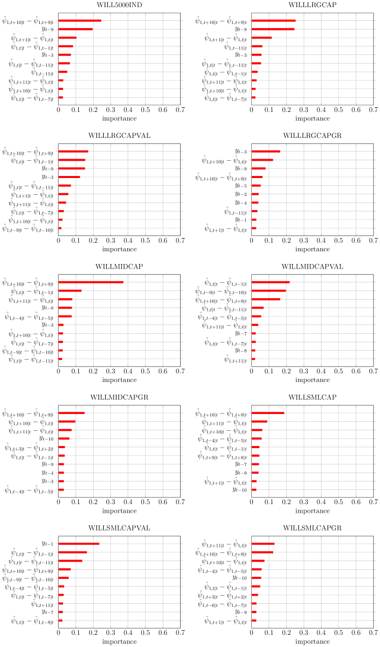
Figure 6: Importance weights post COVID-19: top 10 predictors.

Table 3: Glossary for the acronyms in table 1.

Acronym	Description
BEA	Bureau of Economic Analysis
BLS	Bureau of Labor Statistics
CPI	Consumer Price Index
FRB	Federal Reserve Board
FRBSL	Federal Reserve Bank of St. Louis
TMI	Total Market Index
WA	Wilshire Associates

Table 4: Mean squared errors associated to ridge forecasts, relative to those for naive predictions constant at zero. This is an exact replica of table 2, except for the forecasting model. Indeed, this table uses a ridge regression (with shrinkage selected in an equally spaced grid with cardinality 25 ranging from 0.1 to 100) instead of bootstrap aggregating.

Target	Pre COVID-19			Post COVID-19
	Autoregressive	Augmented		Autoregressive	Augmented
WILL5000IND	0.983	1.041		0.960	3.378
WILLLRGCAP	0.986	1.064		0.960	3.374
WILLLRGCAPVAL	0.944	0.916		0.938	2.843
WILLLRGCAPGR	1.070	1.304		1.015	3.623
WILLMIDCAP	0.996	1.062		0.972	2.436
WILLMIDCAPVAL	0.964	0.936		0.966	1.770
WILLMIDCAPGR	1.081	1.344		1.040	3.375
WILLSMLCAP	0.988	1.065		0.973	2.525
WILLSMLCAPVAL	0.946	0.884		0.944	1.976
WILLSMLCAPGR	1.075	1.459		1.033	3.070

References

• Bańbura and Modugno [2014] M. Bańbura and M. Modugno. Maximum likelihood estimation of factor models on datasets with arbitrary pattern of missing data. Journal of Applied Econometrics, 29(1):133–160, 2014.
• Bańbura et al. [2010] M. Bańbura, D. Giannone, and L. Reichlin. Large bayesian vector auto regressions. Journal of Applied Econometrics, 25(1):71–92, 2010.
• Barigozzi and Luciani [2020] M. Barigozzi and M. Luciani. Quasi maximum likelihood estimation and inference of large approximate dynamic factor models via the em algorithm. arXiv preprint arXiv:1910.03821, 2020.
• Barigozzi and Luciani [2021] M. Barigozzi and M. Luciani. Measuring the output gap using large datasets. The Review of Economics and Statistics, pages 1–45, 2021.
• Barigozzi et al. [2021] M. Barigozzi, M. Lippi, and M. Luciani. Large-dimensional dynamic factor models: Estimation of impulse–response functions with i (1) cointegrated factors. Journal of Econometrics, 221(2):455–482, 2021.
• Bauer and Rudebusch [2016] M. D. Bauer and G. D. Rudebusch. Monetary policy expectations at the zero lower bound. Journal of Money, Credit and Banking, 48(7):1439–1465, 2016.
• Bauer and Rudebusch [2020] M. D. Bauer and G. D. Rudebusch. Interest rates under falling stars. American Economic Review, 110(5):1316–1354, 2020.
• Bernanke et al. [1996] B. Bernanke, M. Gertler, and S. Gilchrist. The financial accelerator and the flight to quality. Review of Economics and Statistics, 78(1):1–15, 1996.
• Bernanke et al. [2005] B. S. Bernanke, J. Boivin, and P. Eliasz. Measuring the effects of monetary policy: a factor-augmented vector autoregressive (favar) approach. The Quarterly journal of economics, 120(1):387–422, 2005.
• Breiman [1996] L. Breiman. Bagging predictors. Machine learning, 24(2):123–140, 1996.
• Breiman [2001] L. Breiman. Random forests. Machine learning, 45(1):5–32, 2001.
• Breiman et al. [1984] L. Breiman, J. Friedman, C. J. Stone, and R. A. Olshen. Classification and regression trees. CRC press, 1984.
• Brown et al. [2022] G. W. Brown, E. Ghysels, and O. Gredil. Nowcasting net asset values: The case of private equity. Review of Financial Studies, forthcoming, 2022.
• Campbell and Diebold [2009] S. D. Campbell and F. X. Diebold. Stock returns and expected business conditions: Half a century of direct evidence. Journal of Business & Economic Statistics, 27(2):266–278, 2009.
• Cimadomo et al. [2022] J. Cimadomo, D. Giannone, M. Lenza, F. Monti, and A. Sokol. Nowcasting with large bayesian vector autoregressions. Journal of Econometrics, 231(2):500–519, 2022.
• Clark [1987] P. K. Clark. The cyclical component of us economic activity. The Quarterly Journal of Economics, 102(4):797–814, 1987.
• Cooper and Priestley [2009] I. Cooper and R. Priestley. Time-varying risk premiums and the output gap. Review of Financial Studies, 22(7):2801–2833, 2009.
• Del Negro et al. [2019] M. Del Negro, D. Giannone, M. P. Giannoni, and A. Tambalotti. Global trends in interest rates. Journal of International Economics, 118:248–262, 2019.
• Dempster et al. [1977] A. P. Dempster, N. M. Laird, and D. B. Rubin. Maximum likelihood from incomplete data via the em algorithm. Journal of the royal statistical society. Series B (methodological), pages 1–38, 1977.
• Doan et al. [1984] T. Doan, R. Litterman, and C. Sims. Forecasting and conditional projection using realistic prior distributions. Econometric reviews, 3(1):1–100, 1984.
• Doz et al. [2012] C. Doz, D. Giannone, and L. Reichlin. A quasi–maximum likelihood approach for large, approximate dynamic factor models. Review of economics and statistics, 94(4):1014–1024, 2012.
• Efron [1979a] B. Efron. Bootstrap methods: Another look at the jackknife. The Annals of Statistics, 7(1):1–26, 1979a.
• Efron [1979b] B. Efron. Computers and the theory of statistics: thinking the unthinkable. SIAM review, 21(4):460–480, 1979b.
• Efron [1981] B. Efron. Nonparametric estimates of standard error: the jackknife, the bootstrap and other methods. Biometrika, 68(3):589–599, 1981.
• Efron and Gong [1983] B. Efron and G. Gong. A leisurely look at the bootstrap, the jackknife, and cross-validation. The American Statistician, 37(1):36–48, 1983.
• Engel and West [2005] C. Engel and K. D. West. Exchange rates and fundamentals. Journal of political Economy, 113(3):485–517, 2005.
• Fama and Schwert [1977] E. F. Fama and G. W. Schwert. Asset returns and inflation. Journal of financial economics, 5(2):115–146, 1977.
• Forni and Lippi [2001] M. Forni and M. Lippi. The generalized dynamic factor model: representation theory. Econometric theory, pages 1113–1141, 2001.
• Forni et al. [2000] M. Forni, M. Hallin, M. Lippi, and L. Reichlin. The generalized dynamic-factor model: Identification and estimation. Review of Economics and statistics, 82(4):540–554, 2000.
• Forni et al. [2005] M. Forni, M. Hallin, M. Lippi, and L. Reichlin. The generalized dynamic factor model: one-sided estimation and forecasting. Journal of the American Statistical Association, 100(471):830–840, 2005.
• Forni et al. [2009] M. Forni, D. Giannone, M. Lippi, and L. Reichlin. Opening the black box: Structural factor models with large cross sections. Econometric Theory, pages 1319–1347, 2009.
• Fries et al. [2018] S. Fries, J.-S. Mésonnier, S. Mouabbi, and J.-P. Renne. National natural rates of interest and the single monetary policy in the euro area. Journal of Applied Econometrics, 33(6):763–779, 2018.
• Gertler and Gilchrist [1994] M. Gertler and S. Gilchrist. Monetary policy, business cycles, and the behavior of small manufacturing firms. The Quarterly Journal of Economics, 109(2):309–340, 1994.
• Geweke [1977] J. F. Geweke. The dynamic factor analysis of economic time series model. Latent variables in socio-economic models, pages 365 – 383, 1977.
• Giannone et al. [2008] D. Giannone, L. Reichlin, and D. Small. Nowcasting: The real-time informational content of macroeconomic data. Journal of Monetary Economics, 55(4):665–676, 2008.
• Giannone et al. [2015] D. Giannone, M. Lenza, and G. E. Primiceri. Prior selection for vector autoregressions. Review of Economics and Statistics, 97(2):436–451, 2015.
• Hamilton et al. [2016] J. D. Hamilton, E. S. Harris, J. Hatzius, and K. D. West. The equilibrium real funds rate: Past, present, and future. IMF Economic Review, 64:660–707, 2016.
• Harvey et al. [1998] A. Harvey, S. J. Koopman, and J. Penzer. Messy time series: a unified approach. Advances in econometrics, 13:103–144, 1998.
• Harvey [1985] A. C. Harvey. Trends and cycles in macroeconomic time series. Journal of Business & Economic Statistics, 3(3):216–227, 1985.
• Harvey [1990] A. C. Harvey. Forecasting, structural time series models and the Kalman filter. Cambridge university press, 1990.
• Hasenzagl et al. [2022a] T. Hasenzagl, F. Pellegrino, L. Reichlin, and G. Ricco. A model of the fed’s view on inflation. The Review of Economics and Statistics, 104(4):686–704, 2022a.
• Hasenzagl et al. [2022b] T. Hasenzagl, F. Pellegrino, L. Reichlin, and G. Ricco. Monitoring the economy in real time: Trends and gaps in real activity and prices. arXiv preprint arXiv:2201.05556, 2022b.
• Hastie et al. [2009] T. Hastie, R. Tibshirani, J. H. Friedman, and J. H. Friedman. The elements of statistical learning: data mining, inference, and prediction, volume 2. Springer, 2009.
• Holston et al. [2017] K. Holston, T. Laubach, and J. C. Williams. Measuring the natural rate of interest: International trends and determinants. Journal of International Economics, 108:S59–S75, 2017.
• Jarociński and Lenza [2018] M. Jarociński and M. Lenza. An inflation-predicting measure of the output gap in the euro area. Journal of Money, Credit and Banking, 50(6):1189–1224, 2018.
• Kim and Singleton [2012] D. H. Kim and K. J. Singleton. Term structure models and the zero bound: an empirical investigation of japanese yields. Journal of Econometrics, 170(1):32–49, 2012.
• Kitagawa and Gersch [1996] G. Kitagawa and W. Gersch. Smoothness priors analysis of time series, volume 116. Springer Science & Business Media, 1996.
• Lawley and Maxwell [1962] D. N. Lawley and A. E. Maxwell. Factor analysis as a statistical method. Journal of the Royal Statistical Society. Series D (The Statistician), 12(3):209–229, 1962.
• Li et al. [2020] D. Li, J. Tosasukul, and W. Zhang. Nonlinear factor-augmented predictive regression models with functional coefficients. Journal of Time Series Analysis, 41(3):367–386, 2020.
• Litterman [1986] R. B. Litterman. Forecasting with bayesian vector autoregressions—five years of experience. Journal of Business & Economic Statistics, 4(1):25–38, 1986.
• Liu and Rubin [1994] C. Liu and D. B. Rubin. The ecme algorithm: a simple extension of em and ecm with faster monotone convergence. Biometrika, 81(4):633–648, 1994.
• Marcellino et al. [2006] M. Marcellino, J. H. Stock, and M. W. Watson. A comparison of direct and iterated multistep ar methods for forecasting macroeconomic time series. Journal of econometrics, 135(1-2):499–526, 2006.
• Meese and Rogoff [1983] R. A. Meese and K. Rogoff. Empirical exchange rate models of the seventies: Do they fit out of sample? Journal of international economics, 14(1-2):3–24, 1983.
• Meng and Rubin [1993] X.-L. Meng and D. B. Rubin. Maximum likelihood estimation via the ecm algorithm: A general framework. Biometrika, 80(2):267–278, 1993.
• Morgan and Sonquist [1963] J. N. Morgan and J. A. Sonquist. Problems in the analysis of survey data, and a proposal. Journal of the American statistical association, 58(302):415–434, 1963.
• Nelson [1976] C. R. Nelson. Inflation and rates of return on common stocks. The journal of Finance, 31(2):471–483, 1976.
• Orphanides and Norden [2002] A. Orphanides and S. v. Norden. The unreliability of output-gap estimates in real time. Review of economics and statistics, 84(4):569–583, 2002.
• Pardo et al. [2013] C. Pardo, J. F. Diez-Pastor, C. García-Osorio, and J. J. Rodríguez. Rotation forests for regression. Applied Mathematics and Computation, 219(19):9914–9924, 2013.
• Pellegrino [2023] F. Pellegrino. Selecting time-series hyperparameters with the artificial jackknife. arXiv preprint arXiv:2002.04697, 2023.
• Quinlan [1986] J. R. Quinlan. Induction of decision trees. Machine learning, 1(1):81–106, 1986.
• Rodriguez et al. [2006] J. J. Rodriguez, L. I. Kuncheva, and C. J. Alonso. Rotation forest: A new classifier ensemble method. IEEE transactions on pattern analysis and machine intelligence, 28(10):1619–1630, 2006.
• Rossi [2013] B. Rossi. Exchange rate predictability. Journal of economic literature, 51(4):1063–1119, 2013.
• Rubin and Thayer [1982] D. B. Rubin and D. T. Thayer. Em algorithms for ml factor analysis. Psychometrika, 47(1):69–76, 1982.
• Särkkä [2013] S. Särkkä. Bayesian filtering and smoothing. Cambridge University Press, 2013.
• Sharpe [1994] S. A. Sharpe. Financial market imperfections, firm leverage, and the cyclicality of employment. The American Economic Review, 84(4):1060–1074, 1994.
• Shumway and Stoffer [1982] R. H. Shumway and D. S. Stoffer. An approach to time series smoothing and forecasting using the em algorithm. Journal of time series analysis, 3(4):253–264, 1982.
• Sims [1980] C. A. Sims. Macroeconomics and reality. Econometrica: journal of the Econometric Society, pages 1–48, 1980.
• Swanson and Williams [2014] E. T. Swanson and J. C. Williams. Measuring the effect of the zero lower bound on medium-and longer-term interest rates. American economic review, 104(10):3154–3185, 2014.
• Watson and Engle [1983] M. W. Watson and R. F. Engle. Alternative algorithms for the estimation of dynamic factor, mimic and varying coefficient regression models. Journal of Econometrics, 23(3):385–400, 1983.