Exploring Low-Cost Transformer Model Compression for Large-Scale Commercial Reply Suggestions

Abstract

Fine-tuning pre-trained language models improves the quality of commercial reply suggestion systems, but at the cost of unsustainable training times. Popular training time reduction approaches are resource intensive, thus we explore low-cost model compression techniques like Layer Dropping and Layer Freezing. We demonstrate the efficacy of these techniques in large-data scenarios, enabling the training time reduction for a commercial email reply suggestion system by $42\%$, without affecting the model relevance or user engagement. We further study the robustness of these techniques to pre-trained model and dataset size ablation, and share several insights and recommendations for commercial applications.

1 Introduction

Automated reply suggestions have become ubiquitous in many popular email and chat applications, such as Outlook Office365 (2018), Teams Microsoft (2020), Gmail Google (2017), and LinkedIn LinkedIn (2017). These systems assist the end-users in responding to a message by providing them multiple short contextually-relevant reply suggestions that can be used to reply with a quick click, thus improving their overall productivity. The dominant techniques for these systems model them as a response selection task Gunasekara et al. (2019) using a bi-encoder matching model that matches the incoming message with a fixed set of pre-selected responses Henderson et al. (2017). Recently, fine-tuning pre-trained Transformer language model encoders such as BERT Devlin et al. (2019), T5 Raffel et al. (2020), or UniLMv2 Bao et al. (2020) has shown improvements in model quality Henderson et al. (2020).

However, commercial reply-suggestion systems can muster massive amounts of training data, which leads to large fine-tuning times for these pre-trained models. Furthermore, commercial systems often stack additional rankers on top, wherein the matching model ranker is used earlier in the stack to retrieve relevant responses, and the latter rankers help induce special attributes like diversity Deb et al. (2019), factual correctness, and user writing style in the responses. For the best model quality, these rankers are often interdependent, and thus a change to a ranker earlier in the stack often requires re-training the entire stack. Additionally, strict compliance with data privacy laws like GDPR EU (2016) requires changing the underlying training dataset every few weeks, requiring all the rankers to be re-trained. These factors make reducing the fine-tuning times of the matching model vital for efficient and continuous development of commercial reply-suggestion systems.

Popular approaches for reducing the training times involve compressing the pre-trained model size using techniques like Distillation Hinton et al. (2015). Such techniques, however, are resource intensive, and require additional training. In this work, we explore low-cost model compression solutions like Layer Dropping and Layer Freezing. We demonstrate that these low-cost techniques are highly effective in large-data scenarios, helping reduce the training times of a commercial email reply suggestion system by over $42\%$. We also show that these techniques can be combined together into a hybrid model for additional gains. We further study the robustness and efficacy of these compression techniques with ablations in the pre-trained model and the training dataset size, and share our findings and recommendations. We hope that these findings will help inform the experimentation and design of commercial applications even beyond reply suggestion scenarios.

Specifically, our findings for large-data scenarios can be summarized as:

1. For the same desired amount of training time reduction, compressing the model and training it on a large dataset preserves the relevance better than training a large model on a downsampled dataset (Section 5.1).

2. Layer Dropping and Layer Freezing are competitive low-cost model compression techniques, and thus should be prioritized over computationally expensive techniques like Distillation (Sections 5.2 and 5.3).

3. A randomly initialized model with sufficient capacity might be able to match the relevance of a pre-trained initialized model at large dataset scale, however, the usage of a pre-trained model is still recommended since it compresses better and can lead to reduced training times (Section 6).

4. However, further improving the pre-trained model through its domain-adaptation doesn’t offer any additional relevance or compression advantages over the vanilla pre-trained model at large dataset scales (Section 6). We thus advise caution before prioritizing improvements to the underlying pre-trained model for task-specific relevance and training time gains.

Similarly, our findings for low-data scenarios can be summarized as:

1. In keeping with the literature, we found that initialization with a pre-trained model is vastly superior to a randomly initialized model of the same capacity. Furthermore, we found that domain-adaptation of the pre-trained model provides additional relevance gains (Section 7). We thus recommend leveraging a pre-trained model and trying out its improvements (for instance its domain-adaptation) in low-data settings.

2. We discovered that the efficacy of model compression techniques can be a function of the size of the fine-tuning dataset. Specifically, we found that Layer Dropping is only competitive on large fine-tuning datasets, whereas the performance of Layer Freezing is agnostic to the dataset size. We thus recommend Layer Freezing over more complex model compression techniques across dataset sizes (Section 7).

We start in section 2 by providing a brief background of our reply suggestion system and the compression techniques being pursued, followed by a brief overview of the related work in section 3. We discuss our experimental setup in section 4, and present the training time reduction results on a large dataset in section 5. We then study the impact of the pre-trained model, and the dataset size in sections 6 and 7 respectively. We discuss future work in section 8, and finally conclude in section 9.

2 Background

2.1 Reply Suggestion System

We model suggesting replies to emails as a retrieval problem from a fixed set of pre-selected candidate responses (a Response Set). Given an email dataset consisting of message-response (MR) pairs, we use a bi-encoder matching architecture to encode the message and response using distinct transformer encoders  Vaswani et al. (2017) (as in Figure 1), and then train the model through a symmetric matching loss Deb et al. (2019) minimization objective between the message and response encodings.

For inference, we rank the responses from the response set using a combination of their matching score with the message (as provided by the bi-encoder), and an additional bias term to promote responses with high pre-computed message-independent LM scores (language model scores). The bias term balances the matching model’s tendency to surface long and highly specific responses by promoting generic responses, and is a hyper-parameter that we tune. We then use lexical clustering to select $3$ diverse responses from the top ranked responses, such that each of the selected responses comes from a different cluster. In our system, we pre-compute and cache the response set encodings, which makes computing the encoding of the incoming message our online serving bottleneck, and incentivizes keeping the message encoder compact. For instance, our baseline system uses $12$ transformer layers to encode the response, and just $6$ to encode the message. This formulation is similar to the work of Henderson et al Henderson et al. (2017).

Our response set consists of a set of responses from our email training dataset that meet a certain frequency threshold are filtered through a set of carefully curated n-grams to prevent them from containing any user information or offensive content. These responses are further reviewed for their quality by a dedicated team of human curators. We use the normalized log frequency of these responses as their message-independent LM score.

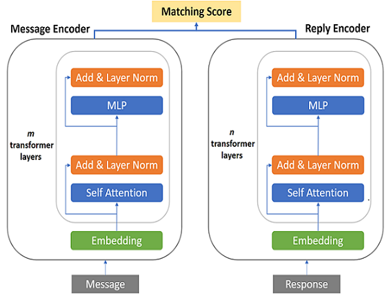
Figure 1: Matching model architecture consisting of a bi-encoder over the message-reply pairs

2.2 Compression Techniques

Literature has shown that pre-trained models are heavily overparameterized, with possible redundancies between layers  Sajjad et al. (2020), and only some subset of the layers needing to be fine-tuned Lee et al. (2019). Thus, several model compression techniques like Distillation, Pruning, and Quantization have been proposed to curb the training times. In this work we investigate the effectiveness of low-cost techniques like Layer Dropping and Freezing.

Layer Dropping: Layer Dropping involves heuristically pruning entire layers from the message and response encoders, and fine-tuning the resulting model. Fewer layers lead to reduced training times and online latencies. Dropping layers also gives the flexibility of selecting which layers to retain from the pre-trained model, and since different layers can capture different linguistic information Tenney et al. (2019); Clark et al. (2019), end-performance can vary based on the layers selected Sajjad et al. (2020).

Layer Freezing: Layer Freezing involves not updating the weights of a bottom few encoder layers during fine-tuning, since the bottom layers usually capture task-agnostic information Lee et al. (2019). This helps reduce the training time by optimizing the backward-pass, however unlike Layer Dropping, it doesn’t provide any inference time reduction.

Note that Layer Dropping and Freezing can additionally be combined together into a Hybrid Model to reap the benefits of both approaches.

2.3 Pre-trained Model

Pre-trained models like BERT Devlin et al. (2019) are trained on large amounts of text from Wikipedia and BookCorpus  Zhu et al. (2015), and thus provide useful representations for many domains. Recently, adaptation of these models to the target domain through continued pre-training  Gururangan et al. (2020) or training from scratch  Gu et al. (2020) has shown to further improve their representations. In this work we study if the domain-adaptation of the pre-trained model leads to better model compression as well.

3 Related Work

Many model compression techniques have been proposed to improve the fine-tuning times of Transformer-based pre-trained models. Distillation Sanh et al. (2019) is a widely used technique where a large pre-trained teacher model is distilled into a smaller student model using a distillation loss. However, pre-trained model distillation can be computationally expensive, thus making it unsuitable for catering to the ad-hoc model size reduction needs of various scenarios. Our work instead explores simple model compression techniques like Layer Dropping and Layer Freezing Sajjad et al. (2020); Lee et al. (2019) that incur no additional computation overhead, and (unlike Distillation) seamlessly support ad-hoc model size reductions by not requiring the pre-trained model to be first distilled down to the desired model size.

Our Layer Dropping technique can also be considered to be a special case of existing techniques like weight or attention head pruning Raganato et al. (2020); Gordon et al. (2020), wherein we heuristically prune entire layers instead of pruning specific weights or attention heads.

Most model compression techniques in literature have been evaluated on public datasets with only modest amounts of fine-tuning data, which is not representative of the scale of fine-tuning datasets available for commercial applications. In this work, we take the first step by evaluating simple model compression techniques on large amounts of fine-tuning data, and study their efficacy with variations in the size of the fine-tuning dataset.

Furthermore, our experiments with the domain-adapted pre-trained model are motivated by their recent success in the literature Gururangan et al. (2020), wherein they have been found to perform better than their vanilla counterparts. However, similar to model compression techniques, the domain-adapted pre-trained models have only been evaluated on tasks with small amounts of fine-tuning data. Our work complements the existing work by experimenting with domain-adapted pre-trained models with varying amount of fine-tuning dataset. We additionally study if domain-adapted pre-trained models offer any model compression advantages.

4 Experimental Setup

Notation: We use $M_{x}R_{y}$ to denote a base matching model with $x$ and $y$ transformer blocks in the message and response encoders respectively. Furthermore, whenever we freeze some layers of the $M_{x}R_{y}$ base model, we will embellish the notation as $(M_{x}R_{y},fm_{i}r_{j})$ to denote that the subword embeddings and the bottom-most $i$ message and $j$ response encoder layers have been frozen during training. We will represent freezing just the subword embeddings on both encoders as $(M_{x}R_{y},f_{emb})$. For Layer Freezing configurations, whenever the base model is clear from the context, we will drop the base model notation and will refer to the model with just the freezing notation $fm_{i}r_{j}$.

Baseline Model: We use a BERT-base bi-encoder architecture Devlin et al. (2019), with $6$ Transformer layers in the message encoder and $12$ in the response ($M_{6}R_{12}$) encoder to keep our serving latencies small. We don’t share weights between the encoders during training, use the CLS token’s output for scoring responses, use the same segment id (of $0$) in both the encoders, a wordpiece uncased vocab of size $30k$, and initialize the weights of encoders with a pre-trained BERT base-like model, called Turing-NLR (TNLR), from Microsoft Turing.

Training: Unless otherwise stated, we train on roughly $60$ million message-reply (MR) pairs extracted from the mailboxes of users of a popular email client. We adhere to strict user privacy policies, and use state-of-the-art privacy preserving technologies. The user data is always kept encrypted, and the model training is carried in a secure environment that doesn’t allow any viewing of the contents of the mailboxes. We use $16$ Nvidia V100 GPUs with InfiniBand connectivity for distributed training. We use gradient accumulation and mixed precision training to speed up the training, and use the Adam optimizer with a scheduled learning rate, involving a linear warmup followed by an exponential decay. We train for a max of $20$ epochs and use validation on $20k$ instances to select the best checkpoint.

Evaluation: The objective of this work is to reduce the training times for our baseline $M_{6}R_{12}$ while maintaining the relevance of the model.

For measuring training time improvements, we use Wall-Clock (WC) time, which we define as the time taken to obtain the best model checkpoint. This depends on the epoch time and the rate of convergence of the model.

For measuring the model relevance offline, we compute a w-Rouge measure on a set of $500k$ email-reply pairs. We define w-Rouge as a weighted version of the Rouge F-measure Lin (2004) that can measure similarity between a user’s actual (golden) response and multiple predicted responses (a response block). For each MR pair instance, we first compute the maximum Rouge-n score between the golden response ($r^{*}$) and each of the $3$ predicted responses ($r_{i}$). We define it as Rouge-n_max (equation 1), where $n$ is the length of the ngram. We then take a weighted average ($w_{n}$ being the weight) of these Rouge-n_max scores across n-grams of length 1, 2, and 3 as in equation 2. We ultimately macro-average these w-Rouge scores across all test instances.

$$\operatorname{{Rouge-n_{max}}}=\max_{i\in\{1,3\}}\operatorname{Rouge-n_{(r^{*},r_{i})}}$$ (1)

$$\operatorname{w-Rouge}={\sum_{n=1}^{3}} w_{n}\times\operatorname{Rouge-n_{max}}$$ (2)

We use w-Rouge over other IR metrics like Mean Reciprocal Rank, since it allows partial overlap, and has demonstrated a higher correlation with our user engagement metrics. We run two-sided T-tests, and only report statistically significant changes where p-value $\leq 0.05$.

The ultimate evaluation of the impact on model relevance is through end-user engagement, for which we divide users into treatment and control groups and conduct experiments with a small percentage of online user traffic. We use user-averaged click-through-rate (CTR) as our engagement metric, and only report statistically significant changes to the CTR (p-value $\leq 0.05$). We thus seek a model with significantly smaller WC time and no drop in online CTR compared to the baseline $M_{6}R_{12}$.

However, since running online experiments is costly and affects the user experience, we run them only for the most promising models with no w-Rouge drop, and use w-Rouge to make inferences for the rest.

Pre-trained Models: We experiment with $3$ pre-trained models – Random (i.e. no pre-training), TNLR, and D-TNLR.

TNLR is Project Turing’s BERT-base equivalent which is trained from scratch similar to BERT, but with the addition of phrase-level masking and replacement of NSP loss with a ‘Sentence Order Prediction (SOP)’ loss. We use TNLR since it has demonstrated improvements over BERT-base on the GLUE dev set Wang et al. (2018).

D-TNLR is the domain-adapted version of TNLR. It is trained from scratch like TNLR on a combination of public datasets and domain-specific commercial email datasets. All training was done in a fully-compliant eyes-off manner, with data given the proper privacy permissions to be used in training and validation. D-TNLR upsamples the email corpus during training, interleaves batches between datasets, and has a performance competitive to TNLR on the GLUE dev set.

5 Results & Discussion

BERT vs TNLR: We first fine-tune and compare the public BERT-base and TNLR baseline models for our task. We see in Table 1 that in addition to similar GLUE scores, the pre-trained models are identical for our task as well (we use $\dagger$ to represent stat-sig. changes throughout). We can thus expect our findings from TNLR to generalize to BERT as well.

Initialization	w-Rouge
BERT	$0.07232$
TNLR	$0.07261$

Table 1: Comparison of TNLR & BERT on $M_{6}R_{12}$

5.1 Dataset Downsampling

We evaluate downsampling the training dataset as a viable training time reduction technique. Table 2 shows that a $90\%$ sample ($54M$) shows no drop in w-Rouge, but yields only a modest time reduction ($16\%$). However, when we sample more aggressively ($\leq 40\%$ or $\leq 25M$), we see a statistically significant $\geq 1.9\%$ drop in w-Rouge. This shows that we can’t rely on downsampling for our desired amounts of training time reduction, while maintaining relevance.

Dataset size	Time	w-Rouge
$60M$	$55.8$hrs	$0.07261$
$54M$	$46.8$hrs	$0.07227$
$25M$	$22.8$hrs	$0.07123^{\dagger}$
$5M$	$25.7$hrs	$0.06919^{\dagger}$
$100k$	$9.6$hrs	$0.05933^{\dagger}$

Table 2: Impact of Dataset Downsampling (#MR pairs)

5.2 Layer Dropping

We first quantify the impact of the position of the layers being retained from the pre-trained model. Towards this goal, we benchmark retaining different layers ($0$ indexed) in the message encoder of a $M_{3}R_{12}$ model compressed with Layer Dropping – Bottom-$3$ (Layers $0,1,2$), Top-$3$ (Layers $9,10,11$), Even-$3$ (Layers $0,6,10$), and Odd-$3$ (Layers $1,7,11$). Table 3 shows that different layer selections are comparable, and thus we consistently use the Odd layer selection in the rest of the Layer Dropping experiments, since it yields slightly better performance.

Layers	w-Rouge
Bottom-3	$0.07221$
Top-3	$0.07232$
Even-3	$0.07216$
Odd-3	$0.07252$

Table 3: Impact of Layer Selection on $M_{3}R_{12}$

Offline Results: We experimented with various degrees of Layer Dropping in the message and response encoders, and found the WC times to go down as we removed more layers (Table 4). We found several configurations with no drop in w-Rouge, with $M_{3}R_{3}$ standing out with 48% fewer parameters, and a 42.3% training time reduction. Further removal of layers, as in with $M_{2}R_{2}$, led to a substantial $1.5\%$ drop in w-Rouge.

Model	#Params	Time	w-Rouge
$M_{6}R_{12}$	$176M$	$55.8$hrs	$0.07261$
$M_{3}R_{12}$	$155M$	$46.2$hrs	$0.07252$
$M_{3}R_{6}$	$113M$	$36.3$hrs	$0.07238$
$M_{3}R_{3}$	$91M$	$32.2$hrs	$0.07225$
$M_{2}R_{2}$	$77M$	$27.3$hrs	$0.07148^{\dagger}$

Table 4: Performance of Layer Dropping

Online Results: Seeing favorable offline results for $M_{3}R_{3}$, we ran an online experiment comparing this model against the baseline for several weeks using real user traffic, and noticed no impact on the CTR – indicating an equal preference for the compressed model. This reduction in model size also helped us reduce our online serving latencies by over 35%, thus saving compute for other parts of the model stack.

5.3 Layer Freezing

Offline Results: We experimented with freezing message and response encoders of $M_{6}R_{12}$ to various degrees (Table 5), and noticed WC times to drop as we froze more layers. #Params in (Table 5) denotes the number of trainable parameters after Layer Freezing. We noticed a significant drop of $75\%$ in w-Rouge when we froze the entire model, thus showing the importance of task-specific fine-tuning. We found several configurations with no drop on w-Rouge, with $fm_{3}r_{6}$ standing out with 63% fewer parameters, and 42.7% reduction in the training time.

Config	#Params	Time	w-Rouge
Unfrozen	176M	55.8hrs	$0.07261$
All frozen	0	0m	$0.01786^{\dagger}$
$fm_{3}r_{0}$	131M	48.8hrs	$0.07291$
$f_{emb}$	129M	46.3hrs	$0.07345$
$fm_{0}r_{6}$	110M	40.8hrs	$0.07270$
$fm_{3}r_{3}$	86M	36.5hrs	$0.07246$
$fm_{3}r_{6}$	$65M$	$32$hrs	$0.07243$
$fm_{6}r_{6}$	43M	27.3hrs	$0.05702^{\dagger}$
$fm_{3}r_{12}$	22M	25.3hrs	$0.06192^{\dagger}$

Table 5: Performance of Layer Freezing on $M_{6}R_{12}$

Online Results: Similar to Layer Dropping, we ran an online experiment comparing $fm_{3}r_{6}$ against the baseline for several weeks, and noticed no impact on the CTR. However, since Layer Freezing has no inference time advantages, we noticed no reduction in our online serving latencies.

Overall, these results demonstrate that Layer Dropping and Layer Freezing are effective and comparable training time reduction techniques on large datasets, with Layer Dropping holding an edge due to its inference time advantages as well. These techniques are complementary to each other and thus can be combined into a hybrid model for additional gains as well. Our initial experiments with hybrid models show that it is possible to further freeze the subword embeddings of the $M_{3}R_{3}$ model without affecting w-Rouge to obtain a cumulative training time reduction of $59\%$ (Table 6).

Model	Time	w-Rouge
$M_{6}R_{12}$	$55.8$hrs	$0.07261$
$(M_{3}R_{3},f_{emb})$	$22.8$hrs	$0.07200$
$(M_{3}R_{3},fm_{1}r_{1})$	$21.5$hrs	$0.07129^{\dagger}$

Table 6: Performance of Hybrid $M_{3}R_{3}$ models

Lastly, we note that our best compressed model $(M_{3}R_{3},f_{emb})$ has a better w-Rouge ($1.1\%$ better) and comparable WC time to training the baseline model $M_{6}R_{12}$ on the downsampled $25M$ dataset (section 5.1). This result suggests that when faced with the need to bring down training times of large models on large datasets, compressing the model and training it on a large dataset preserves the relevance better than training the large model on a downsampled dataset.

6 Impact of Pre-trained Models

Random Initialization: We first benchmark random initialization against TNLR to study the benefits of using a pre-trained model. We see in Table 7 that the Random $M_{6}R_{12}$ baseline performs as well as its TNLR counterpart (p-value: $0.23$). This shows that the relevance benefits of a high-capacity pre-trained model diminish on large datasets. However, the pre-trained model is still desirable because of its higher compressibility, since we found Layer Dropping to not work as well for the randomly initialized model (Table 7). Specifically, the Random $M_{3}R_{3}$ configuration showed a significant drop in w-Rouge of $1.3\%$ compared to TNLR $M_{3}R_{3}$.

Init.	$M_{6}R_{12}$	$M_{3}R_{3}$	$fm_{3}r_{6}$
TNLR	$0.07261$	$0.07225$	$0.07243$
Random	$0.07217$	$0.07129^{\dagger}$	–
D-TNLR	$0.07261$	$0.07223$	$0.07245$

Table 7: Impact of pre-trained model on various model configurations.

Domain-Adapted Pre-trained Model: We then benchmark D-TNLR to check if a better, domain-adapted pre-trained model can help us compress even more. We report in Table 7 that the D-TNLR $M_{6}R_{12}$ baseline performs only as well as its TNLR counterpart. We also see that D-TNLR doesn’t provide any compression benefits over TNLR in its Layer Dropping and Layer Freezing configurations. We additionally found D-TNLR to not show any noticeable convergence time benefits as well.

Overall, these results show that even with large fine-tuning datasets, pre-trained models play a role in making compression techniques like Layer Dropping and Freezing competitive. However, improvement to the pre-trained model by adapting it to the target domain does not yield further compression or convergence benefits with such large datasets. Next, we further investigate the generalization of these observations with dataset size variations.

7 Impact of Dataset Size

We create $2$ sampled datasets of sizes $5M$ and $100k$, and fine-tune on them to study the impact of dataset size on the effectiveness of Layer Dropping, Freezing, and pre-trained models.

Layer Dropping: We repeat the TNLR Layer Dropping experiments on these smaller datasets (Section 5.2), and report in Table 8 that Layer Dropping from $M_{6}R_{12}$ to $M_{3}R_{3}$ doesn’t work as well on $5M$ and $100k$ datasets, as it leads to $1.80\%$ and $2\%$ drops in w-Rouge respectively. This shows that in addition to the pre-trained model (Section 6), the effectiveness of Layer Dropping also depends on the availability of a large fine-tuning dataset.

Layer Freezing: The corresponding TNLR freezing experiments (Table 8) show however, that Layer Freezing’s effectiveness is agnostic to the dataset size. Specifically, $fm_{3}r_{6}$ performs as well as the $M_{6}R_{12}$ baseline on the $5M$ set, and even shows a gain in w-Rouge of $2.5\%$ on the $100k$ set, with the likely explanation here being that freezing potentially helps avoid overfitting on smaller datasets.

These results also show that the preference between Layer Dropping and Freezing changes with the dataset size, with freezing becoming the preferred technique on smaller datasets due to its relevance advantages over dropping.

Config	$60M$	$5M$	$100k$
$M_{6}R_{12}$	$0.07261$	$0.06919$	$0.05933$
$M_{3}R_{3}$	$0.07225$	$0.06795^{\dagger}$	$0.05809^{\dagger}$
$fm_{3}r_{6}$	$0.07243$	$0.06926$	$0.06079^{\dagger}$

Table 8: Comparison of w-Rouge across datasets for various TNLR configs

Pre-trained Model: We repeat the experiments of Section 6 on the $5M$ set, and show (Table 9) that compared to TNLR, the Random $M_{6}R_{12}$ baseline has a drop in w-Rouge of $6\%$. This shows that a pre-trained model is necessary for relevance (and not just for compression) on smaller datasets.

Model	$M_{6}R_{12}$	$M_{3}R_{3}$	$fm_{3}r_{6}$
TNLR	$0.06919$	$0.06795$	$0.06926$
Random	$0.06499^{\dagger}$	$0.06447^{\dagger}$	N/A
D-TNLR	$0.06956$	$0.06823$	$0.06978$

Table 9: Comparison of pre-trained models on 5M set

However, we also see in Table 9 that even with $5M$ instances, D-TNLR performs only as well as TNLR. We thus repeat the experiments on the $100k$ set, and report in Table 10 that at this scale, the D-TNLR baseline not only gives a $6.4\%$ w-Rouge improvement over the TNLR baseline, but also compresses better than TNLR as its dropping and freezing configurations provide $3.75\%$ and $2.46\%$ gains over TNLR respectively. These results show that adapting the pre-trained model to the target domain is a viable training time reduction technique on small datasets.

Model	$M_{6}R_{12}$	$M_{3}R_{3}$	$fm_{3}r_{6}$
TNLR	$0.05933$	$0.05809$	$0.06079$
D-TNLR	$0.06312^{\dagger}$	$0.06027^{\dagger}$	$0.06348^{\dagger}$

Table 10: Comparison of TNLR and D-TNLR on 100k

8 Future Work

Since our recommendations and insights are drawn from our bi-encoder based suggested replies system for a large-scale commercial email service, in the future we will evaluate their generalization to other response selection datasets and architectures. Some early experiments on a large-scale commercial chat client are already showing a similar trend. We will also evaluate the generalization of our findings to other tasks with large amounts of fine-tuning data, primarily the scenarios where implicit labels are readily available such as text prediction. We will also experiment with combining other compression methods such as quantization Zafrir et al. (2019), weight pruning Gordon et al. (2020), and attention head pruning Raganato et al. (2020); Michel et al. (2019) with our layer dropping and freezing configurations to further reduce our training times.

9 Conclusion

We showed that Layer Dropping and Layer Freezing are competitive techniques to compress transformer bi-encoders in commercial, large-data scenarios, and that the presence of a pre-trained model is essential for these compression techniques to work well. In particular, we were able to reduce the training times of a commercial email service’s reply-suggestion system by over $42\%$, without affecting the user engagement. The optimal Layer Dropping configuration also led to a $35\%$ improvement in online latency.

Furthermore, we showed that although these strategies perform similarly at large dataset scales, their comparative efficacy changes when dataset size is varied. Specifically, as the size of the fine-tuning data is reduced, while performance can no longer be matched by dropping layers to the same extent, Layer Freezing continues to be competitive, even improving upon the baseline’s performance.

We also showed that the advantages of domain-adapted pre-trained models Gururangan et al. (2020); Gu et al. (2020) diminish in the presence of large fine-tuning datasets. However, as the dataset size is reduced, domain adaptation becomes important again, as it leads to significant relevance and model compression gains. We believe these insights can benefit many such Transformer bi-encoder based models in commercial settings, by helping achieve significant reductions in model training and allowing faster iteration times in deploying model improvements.

References

- Bao et al. (2020) Hangbo Bao, Li Dong, Furu Wei, Wenhui Wang, Nan Yang, X. Liu, Yu Wang, Songhao Piao, Jianfeng Gao, M. Zhou, and H. Hon. 2020. Unilmv2: Pseudo-masked language models for unified language model pre-training. In ICML.
- Clark et al. (2019) Kevin Clark, Urvashi Khandelwal, Omer Levy, and Christopher D. Manning. 2019. What does BERT look at? an analysis of BERT’s attention. In Proceedings of the 2019 ACL Workshop BlackboxNLP: Analyzing and Interpreting Neural Networks for NLP, pages 276–286, Florence, Italy. Association for Computational Linguistics.
- Deb et al. (2019) Budhaditya Deb, Peter Bailey, and Milad Shokouhi. 2019. Diversifying reply suggestions using a matching-conditional variational autoencoder. In Proceedings of the 2019 Conference of the North American Chapter of the Association for Computational Linguistics: Human Language Technologies, Volume 2 (Industry Papers), pages 40–47, Minneapolis, Minnesota. Association for Computational Linguistics.
- Devlin et al. (2019) Jacob Devlin, Ming-Wei Chang, Kenton Lee, and Kristina Toutanova. 2019. BERT: Pre-training of deep bidirectional transformers for language understanding. In Proceedings of the 2019 Conference of the North American Chapter of the Association for Computational Linguistics: Human Language Technologies, Volume 1 (Long and Short Papers), pages 4171–4186, Minneapolis, Minnesota. Association for Computational Linguistics.
- EU (2016) EU. 2016. Regulation (eu) 2016/679 (general data protection regulation) of the european parliament and of the council.
- Google (2017) Google. 2017. Save time with Smart Reply in Gmail.
- Gordon et al. (2020) Mitchell Gordon, Kevin Duh, and Nicholas Andrews. 2020. Compressing BERT: Studying the effects of weight pruning on transfer learning. In Proceedings of the 5th Workshop on Representation Learning for NLP, pages 143–155, Online. Association for Computational Linguistics.
- Gu et al. (2020) Yu Gu, Robert Tinn, Hao Cheng, Michael Lucas, Naoto Usuyama, Xiaodong Liu, Tristan Naumann, Jianfeng Gao, and Hoifung Poon. 2020. Domain-specific language model pretraining for biomedical natural language processing. ArXiv, abs/2007.15779.
- Gunasekara et al. (2019) Chulaka Gunasekara, Jonathan K Kummerfeld, Lazaros Polymenakos, and Walter Lasecki. 2019. Dstc7 task 1: Noetic end-to-end response selection. In Proceedings of the First Workshop on NLP for Conversational AI, pages 60–67.
- Gururangan et al. (2020) Suchin Gururangan, Ana Marasović, Swabha Swayamdipta, Kyle Lo, Iz Beltagy, Doug Downey, and Noah A. Smith. 2020. Don’t stop pretraining: Adapt language models to domains and tasks. In Proceedings of the 58th Annual Meeting of the Association for Computational Linguistics, pages 8342–8360, Online. Association for Computational Linguistics.
- Henderson et al. (2020) Matthew Henderson, Inigo Casaneuva, Nikola Mrksic, Pei-Hao Su, Tsung-Hsien Wen, and Ivan Vulic. 2020. ConveRT: Efficient and accurate conversational representations from transformers. In Findings of the Association for Computational Linguistics: EMNLP 2020. Association for Computational Linguistics.
- Henderson et al. (2017) Matthew L. Henderson, Rami Al-Rfou, Brian Strope, Yun-Hsuan Sung, László Lukács, Ruiqi Guo, Sanjiv Kumar, Balint Miklos, and Ray Kurzweil. 2017. Efficient natural language response suggestion for smart reply. CoRR, abs/1705.00652.
- Hinton et al. (2015) Geoffrey E. Hinton, Oriol Vinyals, and J. Dean. 2015. Distilling the knowledge in a neural network. ArXiv, abs/1503.02531.
- Lee et al. (2019) Jaejun Lee, Raphael Tang, and Jimmy Lin. 2019. What would elsa do? freezing layers during transformer finetuning. ArXiv, abs/1911.03090.
- Lin (2004) Chin-Yew Lin. 2004. ROUGE: A package for automatic evaluation of summaries. In Text Summarization Branches Out, pages 74–81, Barcelona, Spain. Association for Computational Linguistics.
- LinkedIn (2017) LinkedIn. 2017. Building Smart Replies for Member Messages.
- Michel et al. (2019) Paul Michel, Omer Levy, and Graham Neubig. 2019. Are sixteen heads really better than one? In Advances in Neural Information Processing Systems, volume 32, pages 14014–14024.
- Microsoft (2020) Microsoft. 2020. Reimagining virtual collaboration for the future of work and learning.
- Office365 (2018) Office365. 2018. Use intelligent technology in Outlook on the web and Outlook.com.
- Raffel et al. (2020) Colin Raffel, Noam Shazeer, Adam Roberts, Katherine Lee, Sharan Narang, Michael Matena, Yanqi Zhou, Wei Li, and Peter J. Liu. 2020. Exploring the limits of transfer learning with a unified text-to-text transformer. Journal of Machine Learning Research, 21(140):1–67.
- Raganato et al. (2020) Alessandro Raganato, Yves Scherrer, and Jörg Tiedemann. 2020. Fixed encoder self-attention patterns in transformer-based machine translation. In Findings of the Association for Computational Linguistics: EMNLP 2020, pages 556–568, Online. Association for Computational Linguistics.
- Sajjad et al. (2020) Hassan Sajjad, Fahim Dalvi, Nadir Durrani, and Preslav Nakov. 2020. Poor man’s BERT: Smaller and faster transformer models. ArXiv, abs/2004.03844.
- Sanh et al. (2019) Victor Sanh, Lysandre Debut, Julien Chaumond, and Thomas Wolf. 2019. Distilbert, a distilled version of bert: smaller, faster, cheaper and lighter. ArXiv, abs/1910.01108.
- Tenney et al. (2019) Ian Tenney, Dipanjan Das, and Ellie Pavlick. 2019. BERT rediscovers the classical NLP pipeline. In Proceedings of the 57th Annual Meeting of the Association for Computational Linguistics, pages 4593–4601, Florence, Italy. Association for Computational Linguistics.
- Vaswani et al. (2017) Ashish Vaswani, Noam Shazeer, Niki Parmar, Jakob Uszkoreit, Llion Jones, Aidan N Gomez, Ł ukasz Kaiser, and Illia Polosukhin. 2017. Attention is all you need. In Advances in Neural Information Processing Systems, volume 30, pages 5998–6008.
- Wang et al. (2018) Alex Wang, Amanpreet Singh, Julian Michael, Felix Hill, Omer Levy, and Samuel Bowman. 2018. GLUE: A multi-task benchmark and analysis platform for natural language understanding. In Proceedings of the 2018 EMNLP Workshop BlackboxNLP: Analyzing and Interpreting Neural Networks for NLP, pages 353–355, Brussels, Belgium. Association for Computational Linguistics.
- Zafrir et al. (2019) Ofir Zafrir, Guy Boudoukh, Peter Izsak, and M. Wasserblat. 2019. Q8bert: Quantized 8bit bert. ArXiv, abs/1910.06188.
- Zhu et al. (2015) Y. Zhu, Ryan Kiros, R. Zemel, R. Salakhutdinov, R. Urtasun, A. Torralba, and S. Fidler. 2015. Aligning books and movies: Towards story-like visual explanations by watching movies and reading books. 2015 IEEE International Conference on Computer Vision (ICCV), pages 19–27.