Local X-ray Transform on Asymptotically Hyperbolic Manifolds via Projective Compactification

Abstract.

We prove local injectivity near a boundary point for the geodesic X-ray transform for an asymptotically hyperbolic metric even mod $O(\rho^{5})$ in dimensions three and higher.

Dedicated to the memory of Vaughan Jones

1. Introduction

The problem of recovering a function $f$ from its geodesic X-ray transform

$$If(\gamma)=\int_{\gamma}fds,$$ (1.1)

where $\gamma$ is a geodesic of a Riemannian metric $g$ on a Riemannian manifold and $ds$ denotes integration with respect to $g$-arc length, has been studied extensively since the early 20th century, starting with the Radon transform in the 2-dimensional Euclidean space ([Rad17]). Aside from its intrinsic geometric interest, this question arises in numerous applications, including medical, geophysical and ultrasound imaging; for a comprehensive recent survey see [IM19]. A major breakthrough in the study of the geodesic X-ray transform was the proof by Uhlmann-Vasy ([UV16]) of local injectivity near a boundary point on manifolds of dimension at least 3 with strictly convex boundary. In this paper we prove an analog of the Uhlmann-Vasy result on asymptotically hyperbolic manifolds.

Let $(\overline{M}^{n+1},\partial\overline{M})$ be a compact manifold with boundary and $M$ be its interior. A $C^{\infty}$ metric $g$ on $M$ is called asymptotically hyperbolic (AH) if for some (and hence any) smooth boundary defining function $\rho$ (that is, $\rho\big{|}_{\partial\overline{M}}=0$, $\rho>0$ on $M$, $d\rho\big{|}_{\partial\overline{M}}\neq 0$) the Riemannian metric $\overline{g}:=\rho^{2}g$ on $M$ extends to a smooth metric on $\overline{M}$ with the additional property that $\displaystyle|d\rho|^{2}_{\overline{g}}\equiv 1$ on $\partial\overline{M}$. We denote by $h=\overline{g}|_{T\partial\overline{M}}$ the induced metric on $\partial\overline{M}$. As shown in [Maz86], $(M,g)$ is a complete Riemannian manifold with sectional curvatures approaching $-1$ as $\rho\to 0$. The classical example of an AH manifold is the Poincaré ball model of the hyperbolic space of constant sectional curvature $-1$, the manifold being the Euclidean unit ball $\mathbb{B}^{n+1}=\{(x^{1},\dots,x^{n+1})\in\mathbb{R}^{n+1}:|x|<1\}$ with the metric

$$g_{H}:=4\dfrac{\sum_{j=1}^{n+1}(dx^{j})^{2}}{(1-|x|^{2})^{2}}.$$

Interest in the study of AH manifolds has risen in the past 20 years since the AdS/CFT conjecture, proposed in [Mal98], related conformal field theories with gravity theories on AH spaces.

Since a boundary defining function $\rho$ is determined only up to a smooth positive multiple, $g$ determines a conformal family $\mathfrak{c}$ of metrics on the boundary given by $\mathfrak{c}=[h]$. This conformal class of metrics is called the conformal infinity of $g$. In [GL91], Graham and Lee show that for each conformal representative $h\in\mathfrak{c}$ there exists a unique boundary defining function $\rho$ inducing a product decomposition $[0,\varepsilon)_{\rho}\times\partial\overline{M}$ of a collar neighborhood of the boundary such that the metric can be written in the form

$$g=\frac{d\rho^{2}+h_{\rho}}{\rho^{2}},$$ (1.2)

where $h_{\rho}$ is a one-parameter family of metrics on $\partial\overline{M}$, smooth in $\rho$ up to $\rho=0$, with $h_{0}=h$. We say that an AH metric is in normal form if it is written as in (1.2). Note that (1.2) implies that the equality $|d\rho|^{2}_{\overline{g}}=1$ is valid in a neighborhood of $\partial\overline{M}$ instead of just on $\partial\overline{M}$. In this paper we will be concerned with AH metrics that are even mod $O(\rho^{N})$, where $N$ is a positive odd integer. This means that whenever $g$ is written in normal form (1.2) in a neighborhood of $\partial\overline{M}$, one has

$$(\partial_{\rho})^{m}h_{\rho}\big{|}_{\rho=0}=0\text{ for }m\text{ odd, }1\leq m<N.$$ (1.3)

In the case when (1.3) holds for any odd $N>0$ the metric $g$ will be called even. As shown in [Gui05, Lemma 2.1], evenness mod $O(\rho^{N})$ is a well defined property of an AH metric, independent of the chosen conformal representative determining the normal form (1.2).

A unit-speed geodesic $\gamma$ for $g$ is said to be trapped if either $\liminf_{t\to\infty}\rho(\gamma(t))>0$ or $\liminf_{t\to-\infty}\rho(\gamma(t))>0$. If $\gamma$ is not trapped, then $\lim_{t\to\pm\infty}\gamma(t)\in\partial\overline{M}$ exists and $\rho(\gamma(t))=O(e^{-|t|})$. (See [Maz86] or [GGSU19, Lemma 2.3].) In this case we define

$$If(\gamma):=\int_{-\infty}^{\infty}f(\gamma(t))\,dt$$ (1.4)

for $f$ such that the integral converges.

Injectivity of the X-ray transform has been studied in various settings overlapping with AH spaces. Classical results on hyperbolic space viewed as a symmetric space can be found in [Hel11]. More recently, [Leh] and [LRS18] consider injectivity of the X-ray transform in the setting of Cartan-Hadamard manifolds, which are by definition complete, simply connected manifolds of non-positive curvature; the underlying manifolds are diffeomorphic to $\mathbb{R}^{n}$. Injectivity results specifically in the setting of AH manifolds can be found in [GGSU19].

We will focus on (1.4) restricted to a subset of geodesics. If $U\subset\overline{M}$ (typically an open neighborhood of a point $p\in\partial\overline{M}$, or its closure), a geodesic is said to be $U$-local if $\gamma(t)\in U$ for all $t\in\mathbb{R}$ and $\lim_{t\to\pm\infty}\gamma(t)\in U\cap\partial\overline{M}$. The set $\Omega_{U}$ of $U$-local geodesics is nonempty if $U$ is any open neighborhood of a boundary point; this is a consequence of the existence of “short” geodesics (see §2.2 of [GGSU19]).

As we will indicate in Section 3, for $U$ a small neighborhood of a boundary point, the map $f\to If|_{\Omega_{U}}$ can be defined on $\rho^{3/2}L^{2}(U;dv_{\overline{g}})$ with values in an appropriate $L^{2}$ space (here $dv_{\overline{g}}$ denotes the volume form induced by the smooth metric $\overline{g}$ on $\overline{M}$).

Theorem 1.

Let $\overline{M}$ be a manifold with boundary of dimension at least $3$, with its interior endowed with an asymptotically hyperbolic metric $g$ that is even mod $O(\rho^{5})$. Given any neighborhood $O$ in $\overline{M}$ of $p\in\partial\overline{M}$, there exists a neighborhood $U\subset O$ in $\overline{M}$ of $p$ such that $f\to If\big{|}_{\Omega_{U}}$ is injective on $\rho^{3/2}L^{2}(U;dv_{\overline{g}})$.

We expect that local injectivity holds for general asymptotically hyperbolic metrics, but that other techniques will be needed to prove this. Likewise, we expect that the hypothesis $f\in\rho^{3/2}L^{2}(U;dv_{\overline{g}})$ can be weakened.

Our approach is motivated by the following observation. Recall that the Klein model for hyperbolic space is another metric on $\mathbb{B}^{n+1}$ obtained from the Poincaré metric by a change of the radial variable. Geodesics for the Klein model are straight line segments in $\mathbb{R}^{n+1}$ under suitable parametrizations. So the hyperbolic X-ray transform can be identified with the Euclidean X-ray transform applied to a function supported in the unit ball, modulo changing the parameter of integration on each geodesic. This observation has been utilized in the study of the hyperbolic Radon transform, see e.g. [BT93]. There is an analogous relation for even AH metrics. An even AH metric induces what we call an even structure on $(\overline{M},\partial\overline{M})$ subordinate to its smooth structure. This is a subatlas of the atlas defining the smooth structure, with the property that all the transition maps for the even structure are even diffeomorphisms. One can use the even structure to define a new smooth structure $(\overline{M}_{e},\partial\overline{M}_{e})$ on the topological manifold with boundary underlying $(\overline{M},\partial\overline{M})$ by introducing $r=\rho^{2}$ as a new boundary defining function. As outlined at the end of §4 of [FG12], when viewed relative to the smooth structure $(\overline{M}_{e},\partial\overline{M}_{e})$, the metric $g$ is projectively compact in the sense that its Levi-Civita connection is projectively equivalent to a connection $\widehat{\nabla}$ smooth up to the boundary, i.e. its geodesics agree up to parametrization with the geodesics of $\widehat{\nabla}$. The connection $\widehat{\nabla}$ need not be the Levi-Civita connection of a metric as happens on hyperbolic space, but the Uhlmann-Vasy local injectivity result applies also to the X-ray transform for smooth connections, so local injectivity for even AH metrics follows just by quoting [UV16].

The introduction of $r=\rho^{2}$ as a new defining function to pass from $\overline{M}$ to $\overline{M}_{e}$ is a key step in Vasy’s approach to microlocal analysis on even AH manifolds; see [Vas13a, Vas13b, Vas17].

If the AH metric $g$ is not even, one can still introduce an even structure and a corresponding $(\overline{M}_{e},\partial\overline{M}_{e})$ by introducing $r=\rho^{2}$ as a new boundary defining function. But in this case the connection $\widehat{\nabla}$ is no longer smooth up to the boundary: its Christoffel symbols have expansions in $\sqrt{r}$. If $\partial_{\rho}h_{\rho}\big{|}_{\rho=0}\neq 0$ in (1.2), then the Christoffel symbols have $r^{-1/2}$ terms so $\widehat{\nabla}$ is not even continuous up to the boundary. If $\partial_{\rho}h_{\rho}\big{|}_{\rho=0}=0$ but $(\partial_{\rho})^{3}h_{\rho}\big{|}_{\rho=0}\neq 0$, then $\widehat{\nabla}$ has $\sqrt{r}$ terms so it is continuous but not Lipschitz. Our assumption that $g$ is even modulo $O(\rho^{5})$ guarantees that $\widehat{\nabla}$ is at least a $C^{1}$ connection.

In principle one could try to extend directly the proof in [UV16] to the case of a $C^{1}$ connection like $\widehat{\nabla}$. But the microlocal methods do not seem very well suited to such an analysis. Instead we argue by perturbation: $\widehat{\nabla}$ is a perturbation of a smooth connection, and the perturbation gets smaller the closer one gets to the boundary. For the quantitative control needed to carry this out, we need to use not only the local injectivity result of [UV16], but also the associated stability estimate. We briefly indicate how this goes, beginning by describing this stability estimate.

Let $\overline{\nabla}$ be a smooth connection on a manifold with strictly convex boundary $(\overline{M}_{e},\partial\overline{M}_{e})$, of dimension at least 3, let $r$ be a boundary defining function, and $\widetilde{M}$ a closed manifold of the same dimension containing $\overline{M}_{e}$. The authors of [UV16] constructed a one-parameter family of “artificial boundaries” near a point $p\in\partial\overline{M}_{e}$ given by $\hat{x}=-\eta$, where $\hat{x}\in C^{\infty}(\widetilde{M})$ satisfies $\hat{x}(p)=0$ and $d\hat{x}(p)=-dr(p)$, and $\eta>0$, and showed injectivity of the X-ray transform $\overline{I}$ of $\overline{\nabla}$ restricted to geodesics in $\overline{M}_{e}$ entirely contained in $U_{\eta}:=\{\hat{x}\geq-\eta\}\cap\{r\geq 0\}$, for $\eta$ sufficiently small (see Figure 1).

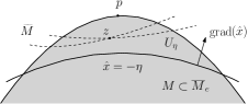
Figure 1. The artificial boundary.

The proof is based on the construction of a family of “microlocalized normal operators” $\overline{A}_{\chi,\eta,\sigma}$ each one of which is, roughly speaking, the conjugate by exponential weights of the average of $\overline{I}f$ over the set of such geodesics passing through a given point. Here $\sigma$ is the parameter in the exponential weight and $\chi$ is a cutoff function. They showed that for appropriately chosen $\chi$, the operator $\overline{A}_{\chi,\eta,\sigma}$ is an elliptic pseudodifferential operator in Melrose’s scattering calculus which for sufficiently small $\eta$ has trivial kernel when acting on functions supported in $U_{\eta}$, and derived the stability estimate

$$\|f\|_{L^{2}(U_{\eta})}\leq C\|\overline{A}_{\chi,\eta,\sigma}f\|_{H_{\operatorname{sc}}^{1,0}(O_{\eta})},$$ (1.5)

where $H_{\operatorname{sc}}^{1,0}$ denotes a scattering Sobolev space and $O_{\eta}$ is a neighborhood of $U_{\eta}$ in $\overline{X}_{\eta}:=\{\hat{x}\geq-\eta\}$.

If $g$ is an AH metric even mod $O(\rho^{N})$, its Levi-Civita connection is projectively equivalent as described above to a connection $\widehat{\nabla}$ of the form $\widehat{\nabla}=\overline{\nabla}+r^{N/2-1}B$ on $\overline{M}_{e}$, where $\overline{\nabla}$ and $B$ are smooth. If $N\geq 5$, then $\widehat{\nabla}$ is $C^{1}$, so the constructions of its X-ray transform $\widehat{I}$ and the operator $\widehat{A}_{\chi,\eta,\sigma}$ can be carried out just as for the smooth connection $\overline{\nabla}$. We show that the norm of the perturbation operator

$$\widehat{A}_{\chi,\eta,\sigma}-\overline{A}_{\chi,\eta,\sigma}:L^{2}(U_{\eta})\to H_{\operatorname{sc}}^{1,0}(O_{\eta})$$ (1.6)

goes to zero as $\eta\to 0$. This gives an estimate of the form (1.5) for $\widehat{A}_{\chi,\eta,\sigma}$ for $\eta$ sufficiently small, which implies local injectivity since $\widehat{A}_{\chi,\eta,\sigma}$ factors through the X-ray transform $\widehat{I}$. The perturbation operator is estimated as in the classical Schur criterion bounding an $L^{2}$ operator norm by the sup of the $L^{1}$ norms of the Schwartz kernel in each variable separately. We lift the kernels of the operators $\widehat{A}_{\chi,\eta,\sigma}$ and $\overline{A}_{\chi,\eta,\sigma}$ to a blown up space which is a refinement of Melrose’s double stretched space (see [Mel94]), where their singularities are more easily analyzed. Due to the fact that the connection $\widehat{\nabla}$ is only of class $C^{1}$, some rather technical analysis is required near each boundary face and corner of the blow-up to conclude that the kernel of $\widehat{A}_{\chi,\eta,\sigma}$ is sufficiently regular that the norm of the perturbation operator vanishes in the limit as $\eta\to 0$.

As in [UV16], the method of proof naturally yields reconstruction via a Neumann series and a stability estimate for $\widehat{I}$ acting between Sobolev spaces on $\overline{M}_{e}$ and the sphere bundle $S^{0}\overline{M}_{e}$ of a smooth metric $g^{0}$ on $\overline{M}_{e}$, which we use to parametrize geodesics for $\widehat{\nabla}$. One could pull back such an estimate to obtain one for $I$ acting between Sobolev spaces on $M$ and the sphere bundle of $g$, but we will not pursue this here. Moreover, one could obtain a global injectivity result in the same way as in [UV16] provided the compact manifold with boundary $\{\rho\geq\varepsilon\}$ admits a strictly convex foliation, for all $\varepsilon$ sufficiently small. We mention that Vasy recently used semiclassical analysis to provide a simplified, compared to [UV16], proof of injectivity of the global and local X-ray transform on compact manifolds with boundary admitting a convex foliation ([Vas]). Global injectivity is shown there without the need for localization and layer stripping. In the present work, working with the local transform is essential for the aforementioned perturbation argument showing Theorem 1 for AH metrics which are even mod $O(\rho^{5})$, and we follow the original formulation of [UV16].

In Section 2 we define even structures on a manifold with boundary and construct the new manifold with boundary $(\overline{M}_{e},\partial\overline{M}_{e})$ obtained by introducing $r=\rho^{2}$ as a new defining function. We show that via this construction, even asymptotically hyperbolic metrics are the same as projectively compact metrics, only viewed relative to different smooth structures near infinity. In Section 3 we use this observation to relate the X-ray transforms for $g$ and $\widehat{\nabla}$, and then deduce Theorem 1 for even AH metrics. Section 4 begins the analysis for the $C^{1}$ connection $\widehat{\nabla}$ arising from an AH metric even mod $O(\rho^{5})$. We decompose $\widehat{\nabla}$ into a smooth projectively compact connection $\overline{\nabla}$ and a nonsmooth error term and extend both to the larger manifold $\widetilde{M}$ in such a way that they agree outside of $M_{e}$. We also prove Lemma 4.1, which states that the exponential map for $\widehat{\nabla}$ has one more degree of regularity than expected. In Section 5 we review scattering Sobolev spaces on a manifold with boundary, the construction of the microlocal normal operator $A_{\chi,\eta,\sigma}$, and the stability estimate (1.5). We also show how Theorem 1 follows from Proposition 5.6, which is the assertion that the norm of the perturbation operator (1.6) goes to zero as $\eta\to 0$. In Section 6 we describe the blown-up double space, analyze in detail the lift of the kernel of $A_{\chi,\eta,\sigma}$ to this space, and conclude with the proof of Proposition 5.6.

Throughout this paper and unless otherwise stated, given an $n+1$-dimensional manifold with boundary (such as $(\overline{M},\partial\overline{M})$ or $(\overline{M}_{e},\partial\overline{M}_{e})$), lower case Latin indices $i$, $j$, $k$ label objects on the manifold and run between $0$ and $n$ in coordinates. Lower case Greek indices $\alpha$, $\beta$, $\gamma$ label objects on the boundary and run between $1$ and $n$ in coordinates. So a Latin index corresponds to a pair $i\leftrightarrow(0,\alpha)$.

2. Even Asymptotically Hyperbolic $=$ Projectively Compact

This paper is based on an equivalence between even asymptotically hyperbolic metrics and projectively compact metrics, briefly outlined at the end of Section 4 of [FG12]. Since it is central to the paper, we describe this equivalence in more detail. We begin by recalling the notions of projective equivalence and projectively compact metrics. A reference for projective equivalence is [Poo81, §5.24].

Two torsion-free connections $\nabla$ and $\widehat{\nabla}$ on a smooth manifold are said to be projectively equivalent if they have the same geodesics up to parametrization. This is equivalent to the condition that their difference tensor $\widehat{\nabla}-\nabla$ is of the form $v_{\!(i}^{\phantom{k}}\delta_{j)}^{k}=\frac{1}{2}(v_{i}\delta_{j}^{k}+v_{j}\delta_{i}^{k})$ for some 1-form $v$. If $\gamma(t)$ is a geodesic for $\nabla$, then $\gamma(t(\tau))$ is a geodesic for $\widehat{\nabla}$, where $t(\tau)$ solves the differential equation $t^{\prime\prime}=\mu(t)(t^{\prime})^{2}$ with $\mu(t)=-v_{\gamma(t)}({\gamma}^{\prime}(t))$. If $v=du$ happens to be exact, then this equation for the parametrization reduces to the first order equation

$$t^{\prime}=ce^{-u(\gamma(t))}$$ (2.1)

which can be integrated by separation of variables.

Let ${}^{e}g$ be a metric on the interior of a manifold with boundary $(\overline{M}_{e},\partial\overline{M}_{e})$. (The explanation for the super/subscript $e$ will be apparent shortly. For now this is just an inconsequential notation.) We say that ${}^{e}g$ is projectively compact if near $\partial\overline{M}_{e}$ it has the form

$${}^{e}g=\frac{dr^{2}}{4r^{2}}+\frac{k}{r},$$

where $r$ is a defining function for $\partial\overline{M}_{e}$ and $k$ is a smooth symmetric 2-tensor on $\overline{M}_{e}$ which is positive definite when restricted to $T\partial\overline{M}_{e}$. (The papers [ČG16a], [ČG16b] consider more general notions of projective compactness; our projectively compact metrics are projectively compact of order $2$ in the terminology introduced there.) It is easily checked that this class of metrics is independent of the choice of defining function $r$. Elementary calculations (see (4.2) below) show that if ${}^{e}\nabla$ is the Levi-Civita connection of such a metric and $r$ a defining function, then the connection $\widehat{\nabla}$ defined by

$$\widehat{\nabla}={}^{e}\nabla+D,\qquad D_{ij}^{k}=v_{(i}^{\phantom{k}}\delta_{j)}^{k},\qquad v=dr/r$$ (2.2)

extends smoothly up to $\partial\overline{M}_{e}$. Thus ${}^{e}\nabla$ is projectively equivalent to the smooth connection $\widehat{\nabla}$. It turns out that projectively compact metrics are the same as even asymptotically hyperbolic metrics upon changing the smooth structure at the boundary. We digress to formulate the notion of an even structure on a manifold with boundary, which underlies this equivalence.

Set $\overline{\mathbb{R}^{n+1}_{+}}=\{(\rho,s):\rho\geq 0,s\in\mathbb{R}^{n}\}$. View $\mathbb{R}^{n}\subset\overline{\mathbb{R}^{n+1}_{+}}$ as the subset $\rho=0$.

Definition 2.1.

Let $\mathcal{U}\subset\overline{\mathbb{R}^{n+1}_{+}}$ be open. Let $f:\mathcal{U}\rightarrow\mathbb{R}$ be smooth. $f$ is said to be even (resp. odd) if either:

1. $\mathcal{U}\cap\mathbb{R}^{n}=\emptyset$, or

2. $\mathcal{U}\cap\mathbb{R}^{n}\neq\emptyset$ and the Taylor expansion of $f$ at each point of $\mathcal{U}\cap\mathbb{R}^{n}$ has only even (resp. odd) terms in $\rho$.

It is equivalent to say that $f$ is even (resp. odd) if there is a smooth function $u$ so that $f(\rho,s)=u(\rho^{2},s)$ (resp. $f(\rho,s)=\rho\,u(\rho^{2},s)$). A smooth map $\varphi:\mathcal{U}\rightarrow\overline{\mathbb{R}^{n+1}_{+}}$ is said to be even if it is of the form $\varphi(\rho,s)=(\rho^{\prime},s^{\prime})$, where $\rho^{\prime}$ is odd and each component of $s^{\prime}$ is even.

Definition 2.2.

Let $(\overline{M},\partial\overline{M})$ be a manifold with boundary, with atlas $\{(\mathcal{U}_{\alpha},\varphi_{\alpha})\}_{\alpha\in\mathcal{A}}$. Let $\{(\mathcal{U}_{\alpha},\varphi_{\alpha})\}_{\alpha\in\widetilde{\mathcal{A}}}$ be a subatlas of $\{(\mathcal{U}_{\alpha},\varphi_{\alpha})\}_{\alpha\in\mathcal{A}}$ corresponding to a subset $\widetilde{\mathcal{A}}\subset\mathcal{A}$. We say that $\{(\mathcal{U}_{\alpha},\varphi_{\alpha})\}_{\alpha\in\widetilde{\mathcal{A}}}$ defines an even structure on $(\overline{M},\partial\overline{M})$ subordinate to its smooth structure if the transition map

$$\varphi_{\alpha_{2}}\circ\varphi_{\alpha_{1}}^{-1}:\varphi_{\alpha_{1}}(\mathcal{U}_{\alpha_{1}}\cap\mathcal{U}_{\alpha_{2}})\rightarrow\varphi_{\alpha_{2}}(\mathcal{U}_{\alpha_{1}}\cap\mathcal{U}_{\alpha_{2}})$$

is even for all $\alpha_{1},\alpha_{2}\in\widetilde{\mathcal{A}}$. The even structure is defined to be the maximal atlas containing $\{(\mathcal{U}_{\alpha},\varphi_{\alpha})\}_{\alpha\in\widetilde{\mathcal{A}}}$ for which all transition maps are even.

Remark 2.3.

Since $\{(\mathcal{U}_{\alpha},\varphi_{\alpha})\}_{\alpha\in\widetilde{\mathcal{A}}}$ is in particular an atlas for the smooth structure determined by $\{(\mathcal{U}_{\alpha},\varphi_{\alpha})\}_{\alpha\in\mathcal{A}}$, the even structure determines the smooth structure with respect to which it is subordinate. So there is really no need to begin with the original smooth structure. Nevertheless, we will usually have the smooth structure to start with and this language is appropriately suggestive. There are many different even structures subordinate to a given smooth structure.

A diffeomorphism for some $\varepsilon>0$ between a collar neighborhood of $\partial\overline{M}$ in $\overline{M}$ and $[0,\varepsilon)\times\partial\overline{M}$ induces an even structure on $(\overline{M},\partial\overline{M})$. In fact, an atlas for $\partial\overline{M}$ induces an atlas for $[0,\varepsilon)\times\partial\overline{M}$ whose transition maps are the identity in the $\rho$ factor and independent of $\rho$ in the $\partial\overline{M}$ factor.

If $(\overline{M},\partial\overline{M})$ is a manifold with boundary with subordinate even structure, it is invariantly defined to say that a function $f$ on $\overline{M}$ is even: $f\circ\varphi_{\alpha}^{-1}$ is required to be even on $\overline{\mathbb{R}^{n+1}_{+}}$ for all charts $(\mathcal{U}_{\alpha},\varphi_{\alpha})$ in the even structure. Likewise for odd functions. Conversely, knowledge of the even and odd functions on $(\overline{M},\partial\overline{M})$ determines the subordinate even structure.

As an aside, we comment that if $(\overline{M},\partial\overline{M})$ is a manifold with boundary, there is a natural one-to-one correspondence between smooth doubles of $(\overline{M},\partial\overline{M})$ and subordinate even structures. Recall that a smooth double of $(\overline{M},\partial\overline{M})$ is a choice of smooth manifold structure on the topological double $2\overline{M}=(\overline{M}\sqcup\overline{M})/\partial\overline{M}$ such that the inclusions $\overline{M}\to 2\overline{M}$ are diffeomorphisms onto their range and such that the natural reflection $2\overline{M}\to 2\overline{M}$ is a diffeomorphism. The even (resp. odd) functions on $(\overline{M},\partial\overline{M})$ are determined by the double by the requirement that their reflection-invariant (resp. anti-invariant) extension to $2\overline{M}$ is smooth.

Denote by $S:\overline{\mathbb{R}^{n+1}_{+}}\rightarrow\overline{\mathbb{R}^{n+1}_{+}}$ the squaring map

$$S(\rho,s)=(\rho^{2},s).$$

Let $(\overline{M},\partial\overline{M})$ be a manifold with boundary and let $\{(\mathcal{U}_{\alpha},\varphi_{\alpha})\}_{\alpha\in\widetilde{\mathcal{A}}}$ define an even structure on $(\overline{M},\partial\overline{M})$ subordinate to its smooth structure. We construct another manifold with boundary $(\overline{M}_{e},\partial\overline{M}_{e})$ as follows. Set $\overline{M}_{e}=\overline{M}$ as topological spaces. Define

$$\psi_{\alpha}=S\circ\varphi_{\alpha},\qquad\alpha\in\widetilde{\mathcal{A}}.$$

If $\alpha_{1}$, $\alpha_{2}\in\widetilde{\mathcal{A}}$, then

$$(\varphi_{\alpha_{2}}\circ\varphi_{\alpha_{1}}^{-1})(\rho,s)=(\rho\,a(\rho,s),s^{\prime}(\rho,s)),$$ (2.3)

where $a$ and the components of $s^{\prime}$ are even. Now $\psi_{\alpha_{2}}\circ\psi_{\alpha_{1}}^{-1}=S\circ(\varphi_{\alpha_{2}}\circ\varphi_{\alpha_{1}}^{-1})\circ S^{-1}$. Hence

$$\begin{split}(\psi_{\alpha_{2}}\circ\psi_{\alpha_{1}}^{-1})(r,s)=&\big{(}S\circ(\varphi_{\alpha_{2}}\circ\varphi_{\alpha_{1}}^{-1})\big{)}(\sqrt{r},s)\\ =&S\big{(}\sqrt{r}\,a(\sqrt{r},s),s^{\prime}(\sqrt{r},s)\big{)}\\ =&\big{(}ra(\sqrt{r},s)^{2},s^{\prime}(\sqrt{r},s)\big{)}.\end{split}$$

Since $a$ and the components of $s^{\prime}$ are even, it follows that $\psi_{\alpha_{2}}\circ\psi_{\alpha_{1}}^{-1}$ is smooth. Hence the charts $\{(\mathcal{U}_{\alpha},\psi_{\alpha})\}_{\alpha\in\widetilde{\mathcal{A}}}$ define a manifold with boundary structure on the topological space $\overline{M}$, which we denote $(\overline{M}_{e},\partial\overline{M}_{e})$. As topological spaces we have $\overline{M}=\overline{M}_{e}$. On the interior, the identity $\mathcal{I}:M\rightarrow M_{e}$ is a diffeomorphism. Since $\psi_{\alpha}\circ\varphi_{\alpha}^{-1}=S$ is smooth, it follows that $\mathcal{I}:\overline{M}\rightarrow\overline{M}_{e}$ is smooth. But $\mathcal{I}^{-1}:\overline{M}_{e}\rightarrow\overline{M}$ is not smooth since in the charts $\psi_{\alpha}$, $\varphi_{\alpha}$, its first component is the function $\sqrt{r}$ on $\overline{\mathbb{R}^{n+1}_{+}}$. The process of passing from $(\overline{M},\partial\overline{M})$ with its subordinate even structure to $(\overline{M}_{e},\partial\overline{M}_{e})$ could be called “introducing $r=\rho^{2}$ as a new boundary defining function”.

Next consider the inverse process of “introducing $\rho=\sqrt{r}$ as a new boundary defining function”. Let $(\overline{N},\partial\overline{N})$ be any manifold with boundary. We construct another manifold with boundary $(\overline{M},\partial\overline{M})$ with subordinate even structure, such that $(\overline{N},\partial\overline{N})$ equals $(\overline{M}_{e},\partial\overline{M}_{e})$ as manifolds with boundary. To do so, let $\{(U_{\alpha},\psi_{\alpha})\}_{\alpha\in\mathcal{A}}$ be an atlas for $(\overline{N},\partial\overline{N})$. Take $\overline{M}=\overline{N}$ as topological spaces. Use as charts on $\overline{M}$ the maps $\varphi_{\alpha}=S^{-1}\circ\psi_{\alpha}$. Now

$$(\psi_{\alpha_{2}}\circ\psi_{\alpha_{1}}^{-1})(r,s)=(rb(r,s),s^{\prime}(r,s))$$

where $b$ and $s^{\prime}$ are smooth. Calculating the compositions as above gives

$$(\varphi_{\alpha_{2}}\circ\varphi_{\alpha_{1}}^{-1})(\rho,s)=\left(\rho\sqrt{b(\rho^{2},s)},s^{\prime}(\rho^{2},s)\right).$$

Since $b(0,s)\neq 0$, this is an even diffeomorphism. The atlas $\{(U_{\alpha},\varphi_{\alpha})\}_{\alpha\in\mathcal{A}}$ thus defines the desired manifold with boundary $(\overline{M},\partial\overline{M})$ with subordinate even structure. In this case the subatlas $\widetilde{\mathcal{A}}$ equals $\mathcal{A}$.

Suppose now that $g$ is an AH metric on the interior $M$ of a compact manifold with boundary $(\overline{M},\partial\overline{M})$ with a subordinate even structure. In the context of this discussion it is natural to define $g$ to be even relative to the chosen even structure if in coordinates $(\rho,s)$ in the even structure it has the form

$$g=\rho^{-2}\big{(}\overline{g}_{00}d\rho^{2}+2\overline{g}_{0\alpha}d\rho ds^{\alpha}+\overline{g}_{\alpha\beta}ds^{\alpha}ds^{\beta}\big{)}$$ (2.4)

with $\overline{g}_{00}$, $\overline{g}_{\alpha\beta}$ even and $\overline{g}_{0\alpha}$ odd. The choice of a representative $h$ for the conformal infinity induces a diffeomorphism between $[0,\varepsilon)\times\partial\overline{M}$ and a collar neighborhood of $\partial\overline{M}$ with respect to which $g$ has the form (1.2) with $h_{0}=h$. By analyzing the construction of the normal form in [GL91], it is not hard to see that this diffeomorphism putting $g$ into normal form is even relative to the coordinates $(\rho,s)$ and the even structure determined by the product $[0,\varepsilon)\times\partial\overline{M}$ (see the proof of [Gui05, Lemma 2.1] for the special case when (2.4) is already in normal form relative to another representative). It follows that $g$ is even as defined in the introduction and that $g$ uniquely determines the even structure with respect to which it is even. In the other direction, an even AH metric in the sense of the introduction is clearly even with respect to the even structure determined by any of its normal forms. Thus an AH metric $g$ is even in the sense of the introduction if and only if it is even relative to some even structure subordinate to the smooth structure on $(\overline{M},\partial\overline{M})$, and this even structure is uniquely determined by $g$.

If $g$ is an even AH metric, we can consider the smooth manifold with boundary $(\overline{M}_{e},\partial\overline{M}_{e})$ obtained from the even structure determined by $g$ upon introducing $r=\rho^{2}$ as a new boundary defining function. Since $\mathcal{I}^{-1}:M_{e}\rightarrow M$ is a diffeomorphism, ${}^{e}g:=(\mathcal{I}^{-1})^{*}g$ is a metric on $M_{e}$. We claim that ${}^{e}g$ is projectively compact relative to the smooth structure on $(\overline{M}_{e},\partial\overline{M}_{e})$. In fact, if $g$ has the form (1.2) on $[0,\varepsilon)\times\partial\overline{M}$ with $h_{\rho}$ even in $\rho$, then

$${}^{e}g=\frac{dr^{2}}{4r^{2}}+\frac{k_{r}}{r},$$ (2.5)

where $k_{r}=h_{\sqrt{r}}$ is a one-parameter family of metrics on $\partial\overline{M}_{e}$ which is smooth in $r$. Thus ${}^{e}g$ is projectively compact. Conversely, a projectively compact metric relative to $(\overline{M}_{e},\partial\overline{M}_{e})$ is an even AH metric when viewed relative to $(\overline{M},\partial\overline{M})$.

In summary, the class of even asymptotically hyperbolic metrics on the interior of a manifold with boundary $(\overline{M},\partial\overline{M})$ with subordinate even structure is exactly the same as the class of projectively compact metrics in the interior of $(\overline{M}_{e},\partial\overline{M}_{e})$. The distinction is just a matter of which smooth structure one chooses to use at infinity. The smooth structures are related by introducing $r=\rho^{2}$ as a new defining function.

3. Local Injectivity for Even Metrics

Let $(\overline{M},\partial\overline{M})$ be a manifold with boundary and $g$ an even AH metric on $M$. As described in Section 2, the associated metric ${}^{e}g$ obtained by introducing $r=\rho^{2}$ as a new defining function is projectively compact. In particular, for any defining function $r$ for $\partial\overline{M}_{e}$, the connection $\widehat{\nabla}$ defined by (2.2) is smooth up to $\partial\overline{M}_{e}$. We will reduce the analysis of the local X-ray transform of $g$ to that for $\widehat{\nabla}$.

Lemma 3.1.

$\partial\overline{M}_{e}$ is strictly convex with respect to $\widehat{\nabla}$.

Proof.

Recall that this means that if $r$ is a defining function for $\partial\overline{M}_{e}$ with $r>0$ in $M_{e}$ and if $\widehat{\gamma}$ is a nonconstant geodesic of $\widehat{\nabla}$ such that $r(\widehat{\gamma}(0))=0$ and $dr\big{(}{\widehat{\gamma}}\,^{\prime}(0)\big{)}=0$, then $\partial_{\tau}^{2}(r\circ\widehat{\gamma})|_{\tau=0}<0$. Write $g$ in normal form (1.2) relative to a conformal representative $h$ on $\partial\overline{M}$, so that ${}^{e}g$ has the form (2.5) on $M_{e}$. Letting $\widehat{\Gamma}^{k}_{ij}$ (resp. ${}^{e}\Gamma_{ij}^{k}$) denote the Christoffel symbols of $\widehat{\nabla}$ (resp. the Christoffel symbols of the Levi-Civita connection ${}^{e}\nabla$ of ${}^{e}g$) an easy calculation (see (4.2) below) shows that ${}^{e}\Gamma^{0}_{\alpha\beta}=2k_{\alpha\beta}=2h_{\alpha\beta}$ on $\partial\overline{M}_{e}$. Since $D^{0}_{\alpha\beta}=0$, we have at $\tau=0$:

$$\partial_{\tau}^{2}(r\circ\widehat{\gamma})=-\widehat{\Gamma}^{0}_{ij}{\widehat{\gamma}}^{i}{}^{\prime}\,{\widehat{\gamma}}^{j}{}^{\prime}\,=-\widehat{\Gamma}^{0}_{\alpha\beta}{\widehat{\gamma}}^{\alpha}{}^{\prime}\,{\widehat{\gamma}}^{\beta}{}^{\prime}\,=-{}^{e}\Gamma^{0}_{\alpha\beta}{\widehat{\gamma}}^{\alpha}{}^{\prime}\,{\widehat{\gamma}}^{\beta}{}^{\prime}\,=-2h_{\alpha\beta}{\widehat{\gamma}}^{\alpha}{}^{\prime}\,{\widehat{\gamma}}^{\beta}{}^{\prime}\,<0.$$

∎

It will be convenient to embed $\overline{M}_{e}$ in a smooth compact manifold without boundary $\widetilde{M}$ and to extend $\widehat{\nabla}$ to a smooth connection on $\widetilde{M}$, also denoted $\widehat{\nabla}$. If $\widehat{\gamma}$ is a geodesic of $\widehat{\nabla}$ with $\widehat{\gamma}(0)\in\overline{M}_{e}$, set $\tau_{\pm}(\widehat{\gamma}):=\pm\sup\{{\tau\geq 0}:\widehat{\gamma}(t)\in\overline{M}_{e}\text{ for }0\leq\pm t\leq\tau\}$. If $U\subset\overline{M}_{e}$ (usually a small neighborhood of $p\in\partial\overline{M}$ or its closure), we define the set $\widehat{\Omega}_{U}$ of $U$-local geodesics of $\widehat{\nabla}$ by

$$\widehat{\Omega}_{U}:=\big{\{}\widehat{\gamma}:|\tau_{\pm}(\widehat{\gamma})|<\infty,\;\;|\tau_{+}(\widehat{\gamma})|+|\tau_{-}(\widehat{\gamma})|>0,\;\;\widehat{\gamma}(t)\in U\text{ for }t\in[\tau_{-}(\widehat{\gamma}),\tau_{+}(\widehat{\gamma})]\big{\}}.$$ (3.1)

Here the requirement $|\tau_{+}(\widehat{\gamma})|+|\tau_{-}(\widehat{\gamma})|>0$ excludes geodesics tangent to $\partial\overline{M}_{e}$.

If $f\in C(\overline{U})$, set

$$\widehat{I}f(\widehat{\gamma})=\int_{\tau_{-}(\widehat{\gamma})}^{\tau_{+}(\widehat{\gamma})}f(\widehat{\gamma}(\tau))\,d\tau,\qquad\widehat{\gamma}\in\widehat{\Omega}_{U}.$$ (3.2)

The $U$-local X-ray transform of $f$ is the collection of all $\widehat{I}f(\widehat{\gamma})$, $\widehat{\gamma}\in\widehat{\Omega}_{U}$.

Recall that the parametrization of a geodesic of any connection on $TM_{e}$ is determined up to an affine change $\tau\to a\tau+b$, $a\neq 0$. Such a reparametrization changes $\widehat{I}f(\widehat{\gamma})$ by multiplication by $|a|^{-1}$. In particular, whether or not $\widehat{I}f(\widehat{\gamma})=0$ is independent of the parametrization. It suffices to restrict attention to geodesics whose parametrization satisfies a normalization condition. For instance, in the next section we fix a background metric $g^{0}$ and require that $|{\widehat{\gamma}}^{\prime}(0)|_{g^{0}}=1$.

Next we relate $I$ and $\widehat{I}$. This involves relating objects on $M$ with objects on $M_{e}$. Since $\mathcal{I}:M\to M_{e}$ is the identity map, this amounts to viewing the same object in a different smooth structure, i.e. in different coordinates near the boundary. We suppress writing explicitly the compositions with the charts $\psi_{\alpha}$, $\varphi_{\alpha}$. So the expression of the identity in these coordinates is $\mathcal{I}(\rho,s)=(\rho^{2},s)$. Likewise, $g$ and ${}^{e}g$ are related in coordinates by setting $r=\rho^{2}$, as in (2.5). If $f$ is a function defined on $M$, we can regard $f$ as a function $f_{e}$ on $M_{e}$, related in coordinates by $f(\rho,s)=f_{e}(\rho^{2},s)$. If $U\subset M$, set $U_{e}=\mathcal{I}(U)$.

If $\gamma(t)$ is a $U$-local geodesic for $g$, it is also a geodesic for ${}^{e}g$. Since ${}^{e}\nabla$ is projectively equivalent to $\widehat{\nabla}$, (2.1) and (2.2) imply that $\widehat{\gamma}(\tau):=\gamma(t(\tau))$ is a geodesic for $\widehat{\nabla}$, where $dt/d\tau=c\big{(}r\circ\gamma(t(\tau))\big{)}^{-1}$. Different choices of $c$ determine different parametrizations; imposition of a normalization condition on the parametrization as mentioned above provides one way to specify $c$ for each geodesic. The relation between $I$ and $\widehat{I}$ follows easily:

$$If(\gamma)=\int_{-\infty}^{\infty}f(\gamma(t))\,dt=|c|\int_{\tau_{-}(\widehat{\gamma})}^{\tau_{+}(\widehat{\gamma})}(r^{-1}f_{e})(\gamma(t(\tau)))\,d\tau=|c|\widehat{I}(r^{-1}f_{e})(\widehat{\gamma}).$$ (3.3)

Section 3.4 of [UV16] shows that if $U_{e}$ is a sufficiently small open neighborhood of $p\in\partial\overline{M}_{e}$, then the $U_{e}$-local X-ray transform for a smooth metric extends to a bounded operator on $L^{2}(U_{e})$ with target space $L^{2}$ of a parametrization of the space of $U_{e}$-local geodesics with respect to a suitable measure. The same argument holds in our setting for a smooth connection such as $\widehat{\nabla}$. We will not make explicit the target $L^{2}$ space since we are only concerned here with injectivity.

Equation (3.3) shows that it is important to understand when $r^{-1}f_{e}\in L^{2}(U_{e})$. Making the change of variable $r=\rho^{2}$ in the integral gives

$$\int(r^{-1}f_{e})^{2}\,drds=2\int(\rho^{-2}f)^{2}\rho\,d\rho ds=2\int(\rho^{-3/2}f)^{2}\,d\rho ds.$$

Thus $r^{-1}f_{e}\in L^{2}(U_{e},drds)$ if and only if $f\in\rho^{3/2}L^{2}(U,d\rho ds)$. In particular, $If(\gamma)=|c|\widehat{I}(r^{-1}f_{e})(\widehat{\gamma})$ provides a definition of $If$ for $f\in\rho^{3/2}L^{2}(U,dv_{\overline{g}})$ consistent with its usual definition.

The main result of [UV16] is local injectivity of the geodesic X-ray transform for a smooth metric on a manifold with strictly convex boundary. However, the proof applies just as well for the X-ray transform for a smooth connection such as $\widehat{\nabla}$. In particular, the construction in the main text of the cutoff function $\chi$ for which the boundary principal symbol is elliptic is also valid for a connection since the right-hand side of the geodesic equation ${\gamma}^{k}\,{}^{\prime\prime}=-\Gamma_{ij}^{k}{\gamma}^{i}\,{}^{\prime}{\gamma}^{j}\,{}^{\prime}$ is a quadratic polynomial in ${\gamma}^{\prime}$. We do not need the extension of Zhou discussed in the appendix of [UV16], although that more general result applies as well. The main result of [UV16] transferred to our setting is as follows.

Theorem 3.2 ([UV16]).

Assume that $\dim\overline{M}_{e}\geq 3$ and let $p\in\partial\overline{M}_{e}$. Every neighborhood $O_{e}$ of $p$ in $\overline{M}_{e}$ contains a neighborhood $U_{e}$ of $p$ so that the $U_{e}$-local X-ray transform of $\widehat{\nabla}$ is injective on $L^{2}(U_{e})$.

Proof of Theorem 1 for $g$ even.

The relation (3.3) shows that $f\in\rho^{3/2}L^{2}(U,dv_{\overline{g}})$ is in the kernel of the $U$-local transform for $g$ if and only if $r^{-1}f_{e}\in L^{2}(U_{e})$ is in the kernel of the $U_{e}$-local transform for $\widehat{\nabla}$. Thus for $g$ even, Theorem 1 follows immediately from Theorem 3.2. ∎

4. Connections Associated to AH Metrics Even mod $O(\rho^{N})$

If the AH metric $g$ in (1.2) is not even, then the even structure on $(\overline{M},\partial\overline{M})$ determined by a normal form for $g$ depends on the choice of normal form. We fix one such normal form and thus the even structure it determines. We then construct $(\overline{M}_{e},\partial\overline{M}_{e})$ as above by introducing $r=\rho^{2}$ as a new boundary defining function. The metric ${}^{e}g$ would be projectively compact except that the corresponding one-parameter family $k_{r}=h_{\sqrt{r}}$ in (2.5) is no longer smooth: it has an expansion in powers of $\sqrt{r}$. The connection $\widehat{\nabla}$ defined by (2.2) involves first derivatives of $k_{r}$. As already discussed in the Introduction, assuming that $g$ is even mod $O(\rho^{5})$ suffices to guarantee that $\widehat{\nabla}$ is Lipschitz continuous, and, in fact, that it extends to be $C^{1}$ up to $\partial\overline{M}_{e}$, though not necessarily $C^{2}$. Near $\partial\overline{M}_{e}$, $\widehat{\nabla}$ can be viewed as a perturbation of a smooth connection $\overline{\nabla}$.

Straightforward calculation from (2.5) shows that the Christoffel symbols of the connection $\widehat{\nabla}$ defined by (2.2) are given in terms of coordinates near a point $p\in\partial\overline{M}_{e}$ by

$$\begin{gathered}\widehat{\Gamma}_{ij}^{0}=\begin{pmatrix}0&0\\ 0&2(k_{\alpha\beta}-r\partial_{r}k_{\alpha\beta})\end{pmatrix},\qquad\widehat{\Gamma}_{ij}^{\gamma}=\begin{pmatrix}0&\tfrac{1}{2}k^{\gamma\delta}\partial_{r}k_{\delta\beta}\\ \tfrac{1}{2}k^{\gamma\delta}\partial_{r}k_{\alpha\delta}&\Gamma_{\alpha\beta}^{\gamma}\end{pmatrix},\end{gathered}$$ (4.2)

where $\Gamma_{\alpha\beta}^{\gamma}$ denotes the Christoffel symbols of $k_{r}$ with $r$ fixed. If $g$ is even mod $O(r^{N})$ with $N$ odd, then $k=k^{(1)}+r^{N/2}k^{(2)}$ with $k^{(1)}$, $k^{(2)}$ smooth. It follows that all $\widehat{\Gamma}_{ij}^{k}$ have the form

$$\widehat{\Gamma}_{ij}^{k}=\overline{\Gamma}_{ij}^{k}+r^{N/2-1}B_{ij}^{k}$$

with $\overline{\Gamma}_{ij}^{k}$, $B_{ij}^{k}$ smooth up to $\partial\overline{M}_{e}$. The expressions $\overline{\Gamma}_{ij}^{k}$, $B_{ij}^{k}$ can be interpreted as the Christoffel symbols of a smooth connection $\overline{\nabla}$ on $\overline{M}_{e}$ and the coordinate expression of a $(1,2)$ tensor field $B$ respectively. $\overline{\nabla}$ and $B$ are not uniquely determined by the connection $\widehat{\nabla}$; henceforth we fix one choice for them. Recall that we have chosen a closed manifold $\widetilde{M}$ containing $\overline{M}_{e}$. Choose some smooth extension of $\overline{\nabla}$ to a neighborhood of $\overline{M}_{e}$, also denoted $\overline{\nabla}$. Then extend $\widehat{\Gamma}$ by

$$\widehat{\Gamma}_{ij}^{k}=\overline{\Gamma}_{ij}^{k}+r^{N/2-1}H(r)B_{ij}^{k}$$ (4.3)

where $H(r)$ is the Heaviside function. The extended connection $\widehat{\nabla}$ is then $C^{(N-3)/2}$ and the two connections $\widehat{\nabla}$, $\overline{\nabla}$ agree outside of $M_{e}$.

An important consequence of the special structure of the connection $\widehat{\nabla}$ is that its exponential map is more regular than one would expect. We consider the exponential map in the form $\widehat{\exp}:T\widetilde{M}\to\widetilde{M}\times\widetilde{M}$, defined by $\widehat{\exp}(z,v)=(z,\widehat{\varphi}(1,z,v))$, where $t\to\widehat{\varphi}(t,z,v)$ is the geodesic with $\widehat{\varphi}(0,z,v)=z$, $\widehat{\varphi}\,^{\prime}(0,z,v)=v$. Since $\widehat{\nabla}$ is $C^{(N-3)/2}$ and $N\geq 5$, usual ODE theory implies that $\widehat{\exp}$ is a $C^{(N-3)/2}$ diffeomorphism from a neighborhood of the zero section onto its image. In fact, it has one more degree of differentiability. We formulate the result in terms of the inverse exponential map since that is how we will use it.

Lemma 4.1.

Let $\widehat{\nabla}$ be the $C^{(N-3)/2}$ connection defined by (4.3), where $N\geq 5$ is an odd integer. Then $\widehat{\exp}^{-1}$ is $C^{(N-1)/2}$ in a neighborhood in $\widetilde{M}\times\widetilde{M}$ of the diagonal in $\partial\overline{M}_{e}\times\partial\overline{M}_{e}$.

Proof.

It suffices to show that $T\widetilde{M}\ni(z,v)\to\widehat{\varphi}(1,z,v)\in\widetilde{M}$ is $C^{(N-1)/2}$ near $(z,0)$ for $z\in\partial\overline{M}_{e}$. Work in coordinates $(r,s)$ for $z$ with respect to which ${}^{e}g$ is in normal form (2.5). Set $z=(z^{0},z^{\alpha})=(r,s^{\alpha})$. For $v$ use induced coordinates $v=(v^{0},v^{\alpha})$ with $v=v^{0}\partial_{r}+v^{\alpha}\partial_{s^{\alpha}}=v^{i}\partial_{z^{i}}$ and set $w=(z,v)$. Write the flow as $\widehat{\varphi}(t,w)=(\widetilde{z}(t,w),\widetilde{v}(t,w))$. The geodesic equations are:

$$(\widetilde{z}\,^{k})^{\prime}=\widetilde{v}\,^{k},\qquad(\widetilde{v}\,^{k})^{\prime}=-\widehat{\Gamma}_{ij}^{k}(\widetilde{z})\widetilde{v}\,^{i}\widetilde{v}\,^{j}.$$ (4.4)

Observe from (4.2) that all $\widehat{\Gamma}_{ij}^{k}$ are $C^{(N-1)/2}$ except for $\widehat{\Gamma}_{0\alpha}^{\gamma}=\widehat{\Gamma}_{\alpha 0}^{\gamma}$. So the right-hand sides of all equations in (4.4) are $C^{(N-1)/2}$ except for the equation for $(\widetilde{v}\,^{\gamma})^{\prime}$. By (4.2), (4.3), this equation has the form

$$(\widetilde{v}\,^{\gamma})^{\prime}=A_{ij}^{\gamma}(\widetilde{z})\widetilde{v}\,^{i}\widetilde{v}\,^{j}-2\widetilde{r}^{N/2-1}H(\widetilde{r})B_{0\beta}^{\gamma}(\widetilde{z})\widetilde{v}\,^{0}\widetilde{v}\,^{\beta}$$ (4.5)

with $A_{ij}^{\gamma}$ of regularity $C^{(N-1)/2}$ and $B_{0\beta}^{\gamma}$ smooth. Using $\widetilde{r}\,^{\prime}=\widetilde{v}\,^{0}$, write

$$-2\widetilde{r}^{N/2-1}H(\widetilde{r})B_{0\beta}^{\gamma}(\widetilde{z})\widetilde{v}\,^{0}\widetilde{v}\,^{\beta}= -\frac{4}{N}\Big{(}\widetilde{r}^{N/2}H(\widetilde{r})\Big{)}^{\prime}B_{0\beta}^{\gamma}(\widetilde{z})\,\widetilde{v}\,^{\beta}$$ (4.6)

$$= -\frac{4}{N}\Big{(}\widetilde{r}^{N/2}H(\widetilde{r})B_{0\beta}^{\gamma}(\widetilde{z})\,\widetilde{v}\,^{\beta}\Big{)}^{\prime}$$ (4.7)

$$\quad+\frac{4}{N}\widetilde{r}^{N/2}H(\widetilde{r})\Big{(}B_{0\beta}^{\gamma}{}_{,k}(\widetilde{z})\,\widetilde{v}\,^{k}\widetilde{v}\,^{\beta}+B_{0\beta}^{\gamma}(\widetilde{z})\,(\widetilde{v}\,^{\beta})^{\prime}\Big{)}$$ (4.8)

$$= -\frac{4}{N}\Big{(}\widetilde{r}^{N/2}H(\widetilde{r})B_{0\beta}^{\gamma}(\widetilde{z})\,\widetilde{v}\,^{\beta}\Big{)}^{\prime}+\frac{4}{N}\widetilde{r}^{N/2}H(\widetilde{r})C_{ij}^{\gamma}(\widetilde{z})\widetilde{v}\,^{i}\widetilde{v}\,^{j},$$ (4.9)

where for the last equality we have used (4.4) for $(\widetilde{v}\,^{\beta})^{\prime}$, so that

$$C_{ij}^{\gamma}(\widetilde{z})\widetilde{v}\,^{i}\widetilde{v}\,^{j}=B_{0\beta}^{\gamma}{}_{,k}(\widetilde{z})\,\widetilde{v}\,^{k}\widetilde{v}\,^{\beta}-B_{0\beta}^{\gamma}(\widetilde{z})\widehat{\Gamma}^{\beta}_{ij}(\widetilde{z})\widetilde{v}^{i}\widetilde{v}^{j}.$$

Note that $\widetilde{r}^{N/2}H(\widetilde{r})C_{ij}^{\gamma}(\widetilde{z})\widetilde{v}\,^{i}\widetilde{v}\,^{j}$ is $C^{(N-1)/2}$.

Therefore (4.5) can be rewritten in the form

$$\Big{(}v^{\gamma}+\frac{4}{N}\widetilde{r}^{N/2}H(\widetilde{r})B_{0\beta}^{\gamma}(\widetilde{z})\,\widetilde{v}\,^{\beta}\Big{)}^{\prime}=\Big{(}A_{ij}^{\gamma}(\widetilde{z})+\frac{4}{N}\widetilde{r}^{N/2}H(\widetilde{r})C_{ij}^{\gamma}(\widetilde{z})\Big{)}\widetilde{v}\,^{i}\widetilde{v}\,^{j}.$$ (4.10)

Now the linear transformation $\widetilde{v}\mapsto\widetilde{b}=L(\widetilde{z})\widetilde{v},$ where $\widetilde{b}\,^{\gamma}=\widetilde{v}\,^{\gamma}+\frac{4}{N}\widetilde{r}^{N/2}H(\widetilde{r})B_{0\beta}^{\gamma}(\widetilde{z})\,\widetilde{v}\,^{\beta}$, is of class $C^{(N-1)/2}$ in $(\widetilde{z},\widetilde{v})$ and is invertible for $\widetilde{r}$ small. Replacing (4.5) by (4.10) in (4.4) and setting $\widetilde{v}=L^{-1}(\widetilde{z})\widetilde{b}$ throughout, we obtain a system of ODE of the form

$$\Big{(}\widetilde{z},\widetilde{v}\,^{0},\widetilde{b}\Big{)}^{\prime}=F\Big{(}\widetilde{z},\widetilde{v}\,^{0},\widetilde{b}\Big{)},$$ (4.11)

where $F$ is $C^{(N-1)/2}$. It follows that the map $(t,z,v)\mapsto\widehat{\varphi}(t,z,v)$ is of class $C^{(N-1)/2}$ upon setting $\widetilde{b}\,^{\gamma}=L^{\gamma}_{\beta}(\widetilde{z})\widetilde{v}\,^{\beta}$. ∎

Lemma 3.1 (the strict convexity of $\partial\overline{M}_{e}$) holds for both $\widehat{\nabla}$ and $\overline{\nabla}$ if $g$ is even mod $O(\rho^{N})$ with $N\geq 5$ odd, with the same proof as before. We define the sets $\widehat{\Omega}_{U}$, $\overline{\Omega}_{U}$ of $U$-local geodesics for $\widehat{\nabla}$ and $\overline{\nabla}$ the same way as before. It will be important to have a common parametrization for the sets of geodesics of $\widehat{\nabla}$ and $\overline{\nabla}$. For this purpose, we will fix a smooth background metric $g^{0}$ on $\widetilde{M}$ (this will be done in Section 5). There is no canonical way of choosing $g^{0}$ and the choice made does not affect the conclusions, but a convenient choice will simplify some computations. Once a metric $g^{0}$ has been fixed, we let $S^{0}\widetilde{M}$ denote its unit sphere bundle. For $v\in S^{0}\widetilde{M}$, denote by $\widehat{\gamma}_{v}$, (resp. $\overline{\gamma}_{v}$) the geodesic for $\widehat{\nabla}$ (resp. $\overline{\nabla}$) with initial vector $v$. We define the $U$-local X-ray transforms for $\widehat{\nabla}$ and $\overline{\nabla}$ just as in (3.2), except now we view them as functions on the subsets of $S^{0}\widetilde{M}$ corresponding to $\widehat{\Omega}_{U}$, $\overline{\Omega}_{U}$:

$$\widehat{I}f(v)=\int_{\tau_{-}(\widehat{\gamma}_{v})}^{\tau_{+}(\widehat{\gamma}_{v})}f(\widehat{\gamma}_{v}(\tau))\,d\tau$$

and similarly for $\overline{I}f(v)$. Sometimes we will use the notation $If(v)$ generically for $\widehat{I}f(v)$ or $\overline{I}f(v)$, or, for that matter, for the $U$-local X-ray transform for any $C^{1}$ connection on a manifold with strictly convex boundary. No confusion will arise with the notation $If(\gamma)$ from Section 3 for the X-ray transform for the AH metric $g$, since we will not be dealing with $g$ again except implicitly in the isolated instance where we deduce Theorem 1.

5. Stability and Perturbation Estimates

We continue to work with the connections $\widehat{\nabla}$ and $\overline{\nabla}$ obtained from an AH metric even mod $O(\rho^{N})$ with $N\geq 5$. From now on it will always be assumed that the dimension of $\overline{M}$ (and thus also of $\overline{M}_{e}$) is at least 3. Since $\overline{\nabla}$ is smooth and $\partial\overline{M}_{e}$ is strictly convex with respect to it, Theorem 3.2 (local injectivity) holds also for $\overline{\nabla}$. As mentioned in the Introduction, in order to deduce local injectivity for $\widehat{\nabla}$ we will use the stability estimate derived in [UV16] for the conjugated microlocalized normal operator $\overline{A}_{\chi,\eta,\sigma}$, formulated in terms of scattering Sobolev spaces. In this section we review those spaces, the construction of the microlocalized normal operator, and the stability estimate proved in [UV16]. Then we formulate our main perturbation estimate (Proposition 5.6) and show how Theorem 1 follows from it. Proposition 5.6 will be proved in Section 6. In this section we work almost entirely on $\overline{M}_{e}$ and its extension $\widetilde{M}$ (with the exception of the very last proof), so we will not be using the subscript $e$ for its various subsets to avoid cluttering the notation.

We now define polynomially weighted scattering Sobolev spaces on a compact manifold with boundary $(\overline{X}^{n+1},\partial\overline{X})$. Let $x$ be a boundary defining function for $\overline{X}$. The space of scattering vector fields, denoted by $\mathcal{V}_{\operatorname{sc}}(\overline{X})$, consists of the smooth vector fields on $\overline{X}$ which are a product of $x$ and a smooth vector field tangent to $\partial\overline{X}$. Thus if $(x,y^{1},\dots,y^{n})$ are coordinates near $p\in\partial\overline{X}$, elements of $\mathcal{V}_{\operatorname{sc}}(\overline{X})$ can be written near $p$ as linear combinations over $C^{\infty}(\overline{X})$ of the vector fields $x^{2}\partial_{x},$ $x\partial_{y^{\alpha}}$, $\alpha=1,\dots,n$. If $k\in\mathbb{N}_{0}$ and $\beta\in\mathbb{R}$ let

$$H_{\operatorname{sc}}^{k,\beta}(\overline{X})=\{u\in x^{\beta}L^{2}(\overline{X}):x^{-\beta}V_{1}\dots V_{m}u\in L^{2}(\overline{X})\text{ for }V_{j}\in\mathcal{V}_{\operatorname{sc}}(\overline{X})\text{ and }0\leq m\leq k\};$$ (5.1)

here $L^{2}$ is defined using a smooth measure on $\overline{X}$ . Note that $H^{0,\beta}_{\operatorname{sc}}(\overline{X})=x^{\beta}L^{2}(\overline{X})$. For $s\geq 0$, $H^{s,\beta}_{\operatorname{sc}}(\overline{X})$ can be defined by interpolation and for $s<0$ by duality, though we will not need this. The norms $\|\cdot\|_{H_{\operatorname{sc}}^{k,\beta}(\overline{X})}$ can be defined by fixing scattering vector fields in coordinate patches on $\overline{X}$ that locally span $\mathcal{V}_{\operatorname{sc}}(\overline{X})$ over $C^{\infty}(\overline{X})$; any different choice of vector fields would result in an equivalent norm. If $U$ is a neighborhood of $p\in\partial\overline{X}$ (or the closure of one) then $H_{\operatorname{sc}}^{k,\beta}(U)$ consists of functions of the form $u\big{|}_{U}$, where $u\in H_{\operatorname{sc}}^{k,\beta}\left(\overline{X}\right)$.

We next review the arguments and results we will need from [UV16], starting with the construction of the artificial boundary mentioned in the introduction.

Lemma 5.1 ([UV16], Sec. 3.1).

Let $p\in\partial\overline{M}_{e}$ and $\nabla$ be a $C^{1}$ connection with respect to which $\partial\overline{M}_{e}$ is strictly convex. There exists a smooth function $\hat{x}$ in a neighborhood $\mathcal{U}$ of $p$ in $\widetilde{M}$ with the properties:

1. $\hat{x}(p)=0$

2. $d\hat{x}(p)=-dr(p)$ (recall that $r$ is a boundary defining function for $\overline{M}_{e}$)

3. Setting $x_{\eta}:=\hat{x}+\eta$, for any neighborhood $\widetilde{O}$ of $p$ in $\widetilde{M}$ there exists an $\eta_{0}$ such that $U_{\eta}:=\{r\geq 0\}\cap\{{x_{\eta}}\geq 0\}\subset\widetilde{O}$ for $\eta\leq\eta_{0}$

4. For $\eta$ near 0 (positive or negative) the set $X_{\eta}:=\{\hat{x}>-\eta\}=\{{x_{\eta}}>0\}\subset\widetilde{M}$ has strictly concave boundary with respect to $\nabla$ locally near $p$.

The level sets of $\hat{x}$ can be seen in Figure 1.

Write $Y_{p}=\{\hat{x}=0\}$; by shrinking $\mathcal{U}$ we can assume that $Y_{p}\cap\mathcal{U}$ is a smooth hypersurface of $\widetilde{M}$. We can then identify a neighborhood of $p$ in $\widetilde{M}$ with $(-\varepsilon,\varepsilon)_{\hat{x}}\times Y_{p}$ for some small $\varepsilon>0$ via a diffeomorphism $\varphi_{0}$ (which can be constructed e.g. using the flow of a vector field transversal to $Y_{p}$). Fixing coordinates $y^{1},\dots,y^{n}$ for $Y_{p}$ centered at $p$, choose the metric $g^{0}$ so that in a neighborhood of $p$ it is Euclidean in terms of coordinates $(\hat{x},y^{1},\dots,y^{n})$.

For $\mathcal{U}^{\prime}$ a small neighborhood of $p$ contained in $\mathcal{U}$ and $\eta\in\mathbb{R}$ small, denote by $\psi_{\eta}:\mathcal{U}^{\prime}\to\widetilde{M}$ the map which in terms of the above identification maps $(x,y)\mapsto(x+\eta,y)$. For a fixed small $0<\delta_{0}\ll\varepsilon$ and $0\leq\eta<\delta_{0}$, we can identify a neighborhood of $\partial\overline{X}_{\eta}$ in $\widetilde{M}$ with $(-\delta_{0},\delta_{0})_{x_{\eta}}\times Y_{p}$ via the diffeomorphism $\varphi_{\eta}=\varphi_{0}\circ\psi_{\eta}$. Note that $g^{0}$ is also Euclidean in terms of coordinates $(x_{\eta},y^{1},\dots,y^{n})$. Moreover, $\overline{X}_{\eta}$ is given locally near its boundary by $[0,\delta_{0})_{x_{\eta}}\times Y_{p}$ in terms of this identification and $\psi_{-\eta}$ maps diffeomorphically a neighborhood of $\partial\overline{X}_{0}$ in $\overline{X}_{0}$ onto one of $\partial\overline{X}_{\eta}$ in $\overline{X}_{\eta}$, with inverse $\psi_{\eta}$. Vectors in $S^{0}_{z}\widetilde{M}$, $z\in\overline{X}_{\eta}$, can be written as $v=\lambda\partial_{{x_{\eta}}}+\omega$, where $\omega\in TY_{p}$ (of course not necessarily of unit length, so our setup slightly differs from the one in [UV16], see Remark 5.4 below). Henceforth, the notation $|v|$ for a vector $v$ will refer to norm with respect to $g^{0}$ (which is Euclidean in our coordinates in the region of interest).

In order to show local injectivity of the X-ray transform, one needs a description of geodesics staying within a given neighborhood:

Lemma 5.2 ([UV16], Section 3.2).

Let $\nabla$ be a $C^{1}$ connection with respect to which $\overline{M}_{e}$ has strictly convex boundary. There exist constants $\widetilde{C}>0$, $0<\delta_{1}<\delta_{2}$, $c_{0}>0$ and $\eta_{0}>0$, and neighborhood $Z_{p}$ of $p$ in $Y_{p}$, such that if $0\leq\eta<\eta_{0}$ and if $\gamma(t)$ is a $\nabla$-geodesic with initial position $z=(x,y)\in[0,c_{0}]_{x_{\eta}}\times\overline{Z}_{p}\subset\overline{X}_{\eta}$ and velocity $v=(\lambda,\omega)\in S^{0}_{z}\widetilde{M}$ satisfying

$$\frac{|\lambda|}{|\omega|}\leq\widetilde{C}\sqrt{x}$$ (5.2)

then one has ${x_{\eta}}\circ\gamma(t)\geq 0$ for $|t|\leq\delta_{2}$ and ${x_{\eta}}\circ\gamma(t)\geq c_{0}$ for $|t|\geq\delta_{1}$. See Fig. 2.

By taking $\eta_{0}\ll c_{0}$ in Lemma 5.2 and by Lemma 5.1 one can always assume that a neighborhood of $U_{\eta}$ in $\overline{X}_{\eta}$ is contained in $[0,c_{0}]_{x_{\eta}}\times\overline{Z}_{p}$, and we will henceforth assume that this is the case. Now let $\delta_{1}$ and $\nabla$ be as in Lemma 5.2 and let $\exp:T\widetilde{M}\to\widetilde{M}$ be the exponential map of $\nabla$. If $v\in S_{z}^{0}\widetilde{M}$ satisfies the assumptions of the lemma and $f$ is continuous and supported in $[0,c_{0})_{x_{\eta}}\times{Z}_{p}$, we have $If(v)=\int_{-\delta_{1}}^{\delta_{1}}f(\exp(tv))dt$, so for all such $v$ and $f$ one can define the X-ray transform by integrating only over a fixed finite interval. The authors of [UV16] consider $If$ only on vectors $v=(\lambda,\omega)\in S_{z}^{0}\widetilde{M}$ satisfying a stronger condition, namely that for some positive constant $C_{2}$ one has $\frac{|\lambda|}{|\omega|}\leq C_{2}x$ with $z=(x,y)\in[0,c_{0})_{x_{\eta}}\times{Z}_{p}$ for $\eta$ sufficiently small, and construct a microlocalized normal operator for $I$. Specifically, with $f$ as before and $\chi\in C_{c}^{\infty}(\mathbb{R})$ with $\chi\geq 0$ and $\chi(0)=1$, let

$${A}_{\chi,\eta}f(z):=\int_{S^{0}_{z}\widetilde{M}}\chi\!\left(\frac{\lambda}{|\omega|x}\right)If(v)d{\mu}_{g^{0}},\quad z=(x,y)\in[0,c_{0})_{x_{\eta}}\times{Z}_{p},$$ (5.3)

where $d{\mu}_{g^{0}}$ is the measure induced on $S^{0}_{z}\widetilde{M}$ by $g^{0}|_{T_{z}\widetilde{M}}$. Note that for any $C_{2}$, $c_{0}$ can be chosen sufficiently small that (5.2) is automatically satisfied in $[0,c_{0})_{x_{\eta}}\times{Z}_{p}$. The constant $C_{2}$ is fixed when $\chi\in C_{c}^{\infty}(\mathbb{R})$ is chosen (see Proposition 5.3 below), and then $c_{0}$, $\eta_{0}$ can be chosen so that the integrand in (5.3) is only supported on vectors corresponding to geodesics staying in $\overline{X}_{\eta}$. Finally for $\sigma>0$ define the conjugated microlocalized normal operator:

$${A}_{\chi,\eta,\sigma}:=x_{\eta}^{-2}e^{-\sigma/{x_{\eta}}}{A}_{\chi,\eta}e^{\sigma/{x_{\eta}}}.$$ (5.4)

We denote this operator in case $\nabla=\overline{\nabla}$ (resp. $\widehat{\nabla}$) by $\overline{A}_{\chi,\eta,\sigma}$ (resp. $\widehat{A}_{\chi,\eta,\sigma}$). In the case of the smooth connection $\overline{\nabla}$ on $\overline{M}_{e}$, for which $\partial\overline{M}_{e}$ is strictly convex, and in dimension $\geq 3$, it was proved in [UV16, Proposition 3.3] that $\overline{A}_{\chi,\eta,\sigma}$ are scattering pseudodifferential operators (in the notation there, $\overline{A}_{\chi,\eta,\sigma}\in\Psi_{sc}^{-1,0}(\overline{X}_{\eta})$). This implies that they also act on scattering Sobolev spaces. The following Proposition contains the stability estimate we will need in terms of such spaces.

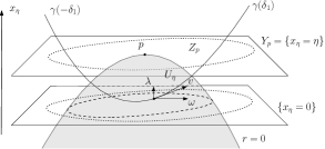
Figure 2. The level sets of $x_{\eta}$

Proposition 5.3 ([UV16], Sections 2.5 and 3.7).

Suppose as before that $\dim(\overline{M}_{e})\geq 3$ and let $\sigma>0$. There exists $\chi_{0}\in C^{\infty}_{c}(\mathbb{R})$, $\chi_{0}\geq 0$, $\chi_{0}(0)=1$, such that for any sufficiently small neighborhood $O$ of $p\in\partial\overline{M}_{e}$ in $\overline{X}_{0}$ there exist $\eta_{0}>0$ and $C_{0}>0$ with the property that for $0\leq\eta\leq\eta_{0}$ one has $U_{\eta}\subset O_{\eta}:=\psi_{-\eta}(O)\subset\overline{X}_{\eta}$, and the estimate

$$\|u\|_{x^{\beta}L^{2}(U_{\eta})}\leq C_{0}\|{\overline{A}}_{\chi_{0},\eta,\sigma}u\|_{H^{1,\beta}_{\operatorname{sc}}(O_{\eta})},\quad\beta\in\mathbb{R},$$ (5.5)

where $u\in x^{\beta}L^{2}(U_{\eta})$ is extended by 0 outside $U_{\eta}$. Here the Sobolev spaces on subsets of $\overline{X}_{\eta}$ are defined by pulling back by $\psi_{\eta}$ the corresponding spaces on subsets of $\overline{X}_{0}$.

Remark 5.4.

The estimate stated in [UV16, Section 3.7] amounts to

$$\|u\|_{H^{s,\beta}_{\operatorname{sc}}(\overline{X}_{\eta})}\leq C_{0}\|{\overline{A}}_{\chi_{0},\eta,\sigma}u\|_{H^{s+1,\beta}_{\operatorname{sc}}(\overline{X}_{\eta})},\quad s\geq 0,\;\operatorname{supp}u\subset U_{\eta},$$ (5.6)

upon taking into account that the analog of $A_{\chi,\eta}$ constructed there has a factor of $x^{-1}$ incorporated and the polynomial factor appearing in the definition of the operator analogous to $A_{\chi,\eta,\sigma}$ is $x_{\eta}^{-1}$, whereas we used a factor of $x_{\eta}^{-2}$ in $A_{\chi,\eta,\sigma}$ directly. For $s=0$ the space on the left hand side of (5.6) is exactly $x^{\beta}L^{2}(U_{\eta})$. On the other hand, the upper bound in (5.6) can be replaced by the one in (5.5) provided $\operatorname{supp}u\subset U_{\eta}$, since the Schwartz kernel of the operators $\overline{A}_{\chi_{0},\eta,\sigma}$ has been localized in both factors near $U_{\eta}$, see for instance [UV16, Remark 3.2].

The way we construct the operators $A_{\chi,\eta}$ also differs from the setup of [UV16] in that we parametrize geodesics by their initial velocities normalized so that they have unit length with respect to the (Euclidean near $p$) metric $g^{0}$, and average the transform over them using the measure induced by $g^{0}$ on the fibers of $S^{0}\widetilde{M}$ (i.e. the standard measure on the unit sphere $\mathbb{S}^{n}$). In [UV16] the geodesics are parametrized by writing their initial velocities as $(\lambda,\omega)\in\mathbb{R}\times\mathbb{S}^{n-1}$ using coordinates, and the measure used for averaging is $d\lambda d\omega$, where $d\omega$ is the standard measure on $\mathbb{S}^{n-1}$. However this difference doesn’t affect the analysis, as already remarked there (see Remark 3.1 and the proof of Proposition 3.3).

Remark 5.5.

As remarked in [UV16, Lemma 3.6], Proposition 5.3 holds for any $\chi_{0}$ sufficiently close to a specific Gaussian in the topology of Schwartz space. In particular, $\chi_{0}$ can be taken to be even, and from now on we assume that this is the case, since this simplifies the notation.

Let $\chi_{0}$ be as in Proposition 5.3, chosen to be even. Let $\sigma>0$ be fixed. Define

$$E_{\eta,\sigma}:=\overline{A}_{\chi_{0},\eta,\sigma}-\widehat{A}_{\chi_{0},\eta,\sigma}$$

Note that by construction the operator $\overline{A}_{\chi_{0},\eta,\sigma}$ (resp. $\widehat{A}_{\chi_{0},\eta,\sigma}$) depends on the behavior of the connection $\overline{\nabla}$ (resp. $\widehat{\nabla}$) only in the set ${x_{\eta}}\geq 0$, provided $\eta_{0}$, $c_{0}$ above are sufficiently small. Therefore $E_{0,\sigma}=0$, since the two connections agree outside of $M_{e}$.

In Section 6.2 we will prove the following key proposition:

Proposition 5.6.

Let $\sigma>0$. Provided $O$ is a sufficiently small neighborhood of $p\in\partial M_{e}$ in $\overline{X}_{0}$, for each $\delta>0$ there exits $\eta_{0}>0$ with the property that if $0\leq\eta<\eta_{0}$ one has $U_{\eta}\subset O_{\eta}=\psi_{-\eta}(O)$ and

$$\|E_{\eta,\sigma}u\|_{H_{\operatorname{sc}}^{1,0}(O_{\eta})}\leq\delta\|u\|_{L^{2}(U_{\eta})}$$ (5.7)

for all $u\in L^{2}(U_{\eta})$ extended by 0 outside of $U_{\eta}$.

Remark 5.7.

In Proposition 5.6 one does not need to assume that $\dim(\overline{M}_{e})\geq 3$, however if $\dim(\overline{M}_{e})=2$ Proposition 5.3 does not hold and the proof of Corollary 5.8 below breaks.

An immediate consequence of Proposition 5.6 is the following:

Corollary 5.8.

With notations as before and assuming that $\dim(\overline{M}_{e})\geq 3$, there exists $\eta_{0}>0$ such that for $0<\eta<\eta_{0}$ the transform $f\mapsto\widehat{I}f\big{|}_{\widehat{\Omega}_{U_{\eta}}}$ is injective on $L^{2}(U_{\eta})$.

Proof.

Fix $\sigma>0$ and let $\chi_{0}$ be as in Proposition 5.3, even. Then take $O$ sufficiently small, as in Propositions 5.3 and 5.6, and let $C_{0}$ and $\eta_{0}$ be according to the former, corresponding to $O$. By Proposition 5.6, upon shrinking $\eta_{0}$ if necessary, for $0\leq\eta<\eta_{0}$ we have

$$\|E_{\eta,\sigma}u\|_{H_{\operatorname{sc}}^{1,0}(O_{\eta})}\leq 1/(2C_{0})\|u\|_{L^{2}(U_{\eta})}$$

for $u\in L^{2}(U_{\eta})$ extended by $0$ elsewhere. Since $\overline{A}_{\chi_{0},\eta,\sigma}=\widehat{A}_{\chi_{0},\eta,\sigma}+E_{\eta,\sigma}$, if $u\in L^{2}(U_{\eta})$ one has, for $0\leq\eta<\eta_{0}$

$$\|u\|_{L^{2}(U_{\eta})}\leq C_{0}\|\overline{A}_{\chi_{0},\eta,\sigma}u\|_{H^{1,0}_{\operatorname{sc}}(O_{\eta})}\leq C_{0}\|\widehat{A}_{\chi_{0},\eta,\sigma}u\|_{H^{1,0}_{\operatorname{sc}}(O_{\eta})}+C_{0}\|E_{\eta,\sigma}u\|_{H^{1,0}_{\operatorname{sc}}(O_{\eta})}$$ (5.8)

$$\quad\leq C_{0}\|\widehat{A}_{\chi_{0},\eta,\sigma}u\|_{H^{1,0}_{\operatorname{sc}}(O_{\eta})}+1/2\|u\|_{L^{2}(U_{\eta})}\Rightarrow\|u\|_{L^{2}(U_{\eta})}\leq 2C_{0}\|\widehat{A}_{\chi_{0},\eta,\sigma}u\|_{H^{1,0}_{\operatorname{sc}}(O_{\eta})}.$$ (5.9)

This implies injectivity of $\widehat{A}_{\chi_{0},\eta,\sigma}$ on $L^{2}(U_{\eta})$. Using the definition of $\widehat{A}_{\chi_{0},\eta,\sigma}$, the local X-ray transform $f\mapsto\widehat{I}f\big{|}_{\widehat{\Omega}_{U_{\eta}}}$ is injective on $e^{\sigma/{x_{\eta}}}L^{2}(U_{\eta})\supset L^{2}(U_{\eta})$ for $0<\eta\leq\eta_{0}$. ∎

Proof of Theorem 1..

The proof presented in Section 3 for the even case applies here verbatim, with the only difference that injectivity of the $U_{e}$-local transform for $\widehat{\nabla}$ on $L^{2}(U_{e})$ now follows from Corollary 5.8. ∎

6. Analysis of Kernels

The goal of this section is to prove Proposition 5.6. In essence, the proof proceeds as for the classical Schur criterion stating that an operator is bounded on $L^{2}$ if its Schwartz kernel is uniformly $L^{1}$ in each variable separately (see e.g. [SR91, Lemma 3.7]). Hence it is necessary to understand well the properties of the kernels of ${\overline{A}}_{\chi_{0},\eta,\sigma}$ and ${\widehat{A}}_{\chi_{0},\eta,\sigma}$. The fine behavior of these kernels is perhaps best analyzed on a modified version of Melrose’s scattering blown-up space ([Mel94]), which we describe in Section 6.1. We then analyze the kernels on it in Section 6.2.

6.1. The Scattering Product

We start by briefly describing blow-ups in general (for a detailed exposition see [Mel]). Let ${Y}^{d}$ be compact manifold with corners and $Z$ a p-submanifold; this means that $Z$ is a submanifold of ${Y}$ with the property that for each $p\in Z$ there exist coordinates for ${Y}$ of the form $(x_{1},\dots,x_{k},y_{1},\dots,y_{d-k})\in\overline{\mathbb{R}}_{+}^{k}\times\mathbb{R}^{d-k}$ centered at $p$, with $x_{j}$ defining functions for boundary hypersurfaces of ${Y}$, such that in terms of them $Z$ is locally expressed as the zero set of a subset of the $x_{i},$ $y_{j}$. If $Z$ is an interior p-submanifold of codimension at least 2, meaning that it is locally given as $y^{\prime}=(y_{j_{1}},\dots,y_{j_{s}})=0$, $2\leq s\leq d-k$ in terms of such coordinates, blowing up $Z$ essentially amounts to introducing polar coordinates in terms of $y^{\prime}$. Formally, let $SN(Z)\overset{\pi}{\to}Z$ be the spherical normal bundle of $Z$ with fiber at $p\in Z$ given by $SN_{p}(Z):=\left((T_{p}{Y}/T_{p}Z)\backslash\{0\}\right)/\mathbb{R}^{+}$. It can be shown that the blown up space $\left[{Y};Z\right]:=SN(Z)\amalg({Y}\backslash Z)$ admits a smooth structure as a manifold with corners such the blow down map $\beta:\left[{Y};Z\right]\to{Y}$, given by $\beta\big{|}_{{Y}\backslash Z}=Id_{{Y}\backslash Z}$ and $\beta\big{|}_{SN(Z)}=\pi$, becomes smooth. The front face of the blown up space is given by $SN(Z)\subset[Y;Z]$. If $Z$ is a boundary p-submanifold, i.e. it is contained in a boundary hypersurface of ${Y}$, the spherical normal bundle is replaced by its inward pointing part, with the rest of the discussion unchanged. If $P$ is a p-submanifold of ${Y}$ that intersects $Z$ with the property $\overline{(P\backslash Z)}=P$, and $\beta$ is a blow down map, then the lift of $P$ is defined as $\beta^{*}(P)=\overline{\beta^{-1}(P\backslash Z)}$. If $\beta=\beta_{1}\circ\cdots\circ\beta_{k}$ with $\beta_{j}$ blow down maps we will write $\beta^{*}(P):=\beta_{k}^{*}(\beta_{k-1}^{*}(\cdots\beta_{1}^{*}(P)))$.

Now let $(\overline{X},\partial\overline{X})$ be a smooth compact manifold with boundary; this implies that $\overline{X}^{2}$ is a smooth manifold with corners. First define the ${\operatorname{b}}$-space $\overline{X}^{2}_{\operatorname{b}}:=\big{[}\overline{X}^{2};(\partial\overline{X})^{2}\big{]}$ with blow down map $\beta_{1}$. We denote by $\operatorname{ff}_{\operatorname{b}}$ the front face of this blow-up. If $\Delta_{\operatorname{b}}:=\overline{\beta^{-1}_{1}(\Delta^{\circ})}$ (the diagonal $\Delta\subset\overline{X}^{2}$ is not a p-submanifold), we let the scattering product be $\overline{X}^{2}_{\operatorname{sc}}:=\big{[}\,\overline{X}_{{\operatorname{b}}}^{2};\partial(\Delta_{\operatorname{b}})\big{]}$ with blow down map $\beta_{2}:\overline{X}^{2}_{\operatorname{sc}}\to\overline{X}^{2}_{\operatorname{b}}$. Set $\beta_{\rm{sc}}=\beta_{1}\circ\beta_{2}$ and let $\operatorname{ff}_{\rm{sc}}\subset\overline{X}_{\rm{sc}}^{2}$ be the front face associated with $\beta_{2}$. We finally introduce a third blown up space obtained from $\overline{X}^{2}_{\rm{sc}}$ by blowing up the scattering diagonal ${{\Delta_{\operatorname{sc}}}}:=\beta_{2}^{*}(\Delta_{\operatorname{b}})$. We denote the new space by $\overline{X}_{\operatorname{d}}^{2}$ and the corresponding blow down map by $\beta_{3}$; let $\beta_{{\operatorname{d}}}:=\beta_{\rm{\operatorname{sc}}}\circ\beta_{3}$. This space is pictured in Fig. 3. By a result on commutativity of blow-ups (see [Mel, Section 5.8]), $\overline{X}_{\operatorname{d}}^{2}$ is diffeomorphic to $\big{[}[\overline{X}_{\operatorname{b}}^{2};\Delta_{\operatorname{b}}],\widetilde{\beta}_{2}^{*}(\partial\Delta_{\operatorname{b}})\big{]}$, where $\widetilde{\beta}_{2}:[\overline{X}_{\operatorname{b}}^{2};\Delta_{\operatorname{b}}]\to\overline{X}^{2}_{\operatorname{b}}$ is the blow down map. We name the various faces of $\overline{X}_{{\operatorname{d}}}^{2}$ as in Fig. 3: $\mathcal{G}_{10}:=\beta_{\operatorname{d}}^{*}\left(\partial\overline{X}\times\overline{X}\right)$, $\mathcal{G}_{01}:=\beta_{\operatorname{d}}^{*}\left(\overline{X}\times\partial\overline{X}\right)$, $\mathcal{G}_{11}:=\beta_{3}^{*}\left(\beta_{2}^{*}\left(\operatorname{ff}_{\operatorname{b}}\right)\right)$ and $\mathcal{G}_{2}:=\beta_{3}^{*}(\operatorname{ff}_{\operatorname{sc}})$; finally let $\mathcal{G}_{3}$ be the front face associated with $\beta_{3}$. We will occasionally write $\mathcal{G}_{\operatorname{b}}$ for the collection of boundary hypersurfaces $\{\mathcal{G}_{10},\mathcal{G}_{11},\mathcal{G}_{01}\}$ and ${\mathcal{G}}_{\operatorname{b}}^{\cup}$ for their union. Moreover, if $p\in\partial\overline{X}$ and $O$ is a neighborhood of $p$ in $\overline{X}$ we let $O^{2}_{\operatorname{d}}:=\beta_{{\operatorname{d}}}^{-1}(O^{2})$.

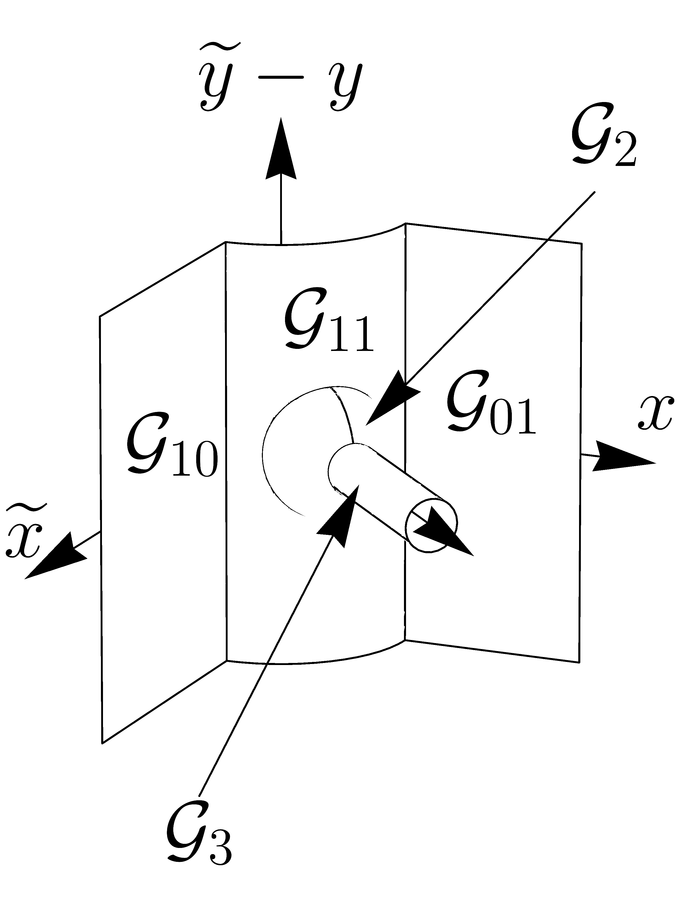
Figure 3. The modified scattering product space $\overline{X}_{{\operatorname{d}}}^{2}$

We next describe the coordinate systems we will use on $\overline{X}^{2}_{\operatorname{d}}$. Let $\dim\left(\overline{X}\right)=n+1$ and $(x,y)$ and $(\widetilde{x},\widetilde{y})$ be two copies of the same coordinate system in a neighborhood $O$ of a point $p\in\partial\overline{X}$, so that $(x,y,\widetilde{x},\widetilde{y})$ is a coordinate system for $O^{2}\subset\overline{X}^{2}$. Here and for the rest of this section $x$ (and thus also $\widetilde{x}$) is a boundary defining function for $\partial\overline{X}$. The projective coordinate systems $(s_{1}=\widetilde{x}/x,x,y,\widetilde{y})$ and $(s_{2}=x/\widetilde{x},\widetilde{x},y,\widetilde{y})$ are valid in a neighborhood of $\mathcal{G}_{01}$ and $\mathcal{G}_{10}$ respectively and the coordinate functions are smooth away from $\mathcal{G}_{10}$ and $\mathcal{G}_{01}$ respectively (though they do not form coordinate systems near $\mathcal{G}_{2}$ and $\mathcal{G}_{3}$ in $\overline{X}^{2}_{\operatorname{d}}$). In terms of the former coordinate system, $s_{1}$ is a defining function for $\mathcal{G}_{01}$ and $x$ a defining function for $\mathcal{G}_{11}$, whereas in terms of the latter $s_{2}$ is a defining function for $\mathcal{G}_{10}$ and $\widetilde{x}$ is one for $\mathcal{G}_{11}$. On the other hand, either by checking directly or by using the commutativity of the blow-up mentioned before, one sees that a valid coordinate system in a neighborhood of any point near $\mathcal{G}_{11}\cap\mathcal{G}_{2}$ can be obtained by appropriately choosing $n$ of the ${\theta}^{j}$ below,

$$\left(\tau=\sqrt{(s_{1}-1)^{2}+|\widetilde{y}-y|^{2}},{\theta}=\frac{(s_{1}-1,\widetilde{y}-y)}{\tau},\sigma=\frac{x}{\tau},y\right),$$ (6.1)

where $|\cdot|$ denotes the Euclidean norm. For instance, letting

$$U_{J}^{\pm}=\big{\{}({\theta}^{0},\dots,{\theta}^{n})\in\mathbb{S}^{n}:\pm{\theta}^{J}>1/\sqrt{2(n+1)}\big{\}},\quad J=0,\dots,n$$ (6.2)

we can cover $\mathbb{S}^{n}$ by the $U_{J}^{\pm}$ and use ${\theta}^{j}$, $j\neq J$ as smooth coordinates on $U_{\pm}^{J}$ for each choice of $\pm$. Now note that $(X=(s_{1}-1)/x,Y=(\widetilde{y}-y)/x,x,y)$ are valid smooth coordinates globally on $(O_{\operatorname{d}}^{2})^{\circ}$, and the coordinate functions are smooth up to $\mathcal{G}_{3}$ and $\mathcal{G}_{2}^{\circ}$. Thus one obtains a diffeomorphism $\mathcal{T}$ from $(O^{2}_{{\operatorname{d}}})^{\circ}$ onto an open subset of $\overline{\mathbb{R}^{n+1}_{+}}\times[0,\infty)\times\mathbb{S}^{n}$, extending to a smooth diffeomorphism up to $\mathcal{G}_{3}$ and $\mathcal{G}_{2}^{\circ}$, by setting

$$\left({x},y,R=\sqrt{X^{2}+|Y|^{2}},{\theta}=(\hat{X},\hat{Y})=\frac{(X,Y)}{R}\right)\in\overline{\mathbb{R}^{n+1}_{+}}\times[0,\infty)\times\mathbb{S}^{n}.$$ (6.3)

Again we can choose coordinates on $\mathbb{S}^{n}$ to obtain smooth valid coordinate systems on $(O_{\operatorname{d}}^{2})^{\circ}$, up to $\mathcal{G}_{3}$ and $\mathcal{G}_{2}^{\circ}$. Note that ${\theta}=({\theta}_{0},\dots,{\theta}_{n})$ stands for the same functions in both (6.1) and (6.3) and that $R$ is a defining function for $\mathcal{G}_{3}$. Moreover,

$$x_{01}= \frac{1+xR\hat{X}}{2+xR\hat{X}},\qquad x_{10}=(2+xR\hat{X})^{-1},\qquad x_{11}=\frac{(2+xR\hat{X})^{2}}{1+R}$$ (6.4)

are smooth defining functions for $\mathcal{G}_{01}$, $\mathcal{G}_{10}$ and $\mathcal{G}_{11}$ respectively, each smooth up to all other boundary hypersurfaces and non-vanishing there.

Via the diffeomorphism $\mathcal{T}$, the expression $|dx\,dy\,dR\,d{\omega}|$ (where $d\omega$ is the volume form on $\mathbb{S}^{n}$ induced by the round metric) pulls back to a smooth global section of the smooth density bundle on $(O_{{\operatorname{d}}}^{2})^{\circ}$, which is smooth and non-vanishing up to $\mathcal{G}_{3}$ and $\mathcal{G}_{2}^{\circ}$, but not up to the other boundary faces. The following can be shown via a straightforward computation in local coordinates smooth up to the various boundary faces in different parts of $O^{2}_{{\operatorname{d}\displaystyle}}$.

Lemma 6.1.

Via the diffeomorphism $\mathcal{T}$ defined by the coordinates (6.3), the expression

$$(R+1)^{-1}(2+xR\hat{X})^{n}|dx\,dy\,dR\,d{\omega}|$$ (6.5)

pulls back to a smooth non-vanishing section of the smooth density bundle on $O^{2}_{{\operatorname{d}}}$, up to all boundary faces.

We now record the form that the lift $\beta_{{\operatorname{d}}}^{*}\widetilde{W}$ takes in terms of (6.3) whenever $\widetilde{W}\in\mathcal{V}_{\operatorname{sc}}(\overline{X})$ is identified with a vector field on $\overline{X}^{2}$ acting on the left factor. (The lift $\beta_{{\operatorname{d}}}^{*}\widetilde{W}$ is well defined since $\beta_{\operatorname{d}}:(\overline{X}^{2}_{\operatorname{d}})^{\circ}\to(\overline{X}^{2}\setminus\Delta)^{\circ}$ is a diffeomorphism.) As before, we work in a neighborhood $O^{2}$ of a point $(p,p)\in\partial\Delta$ where we have coordinates $(x,y,\widetilde{x},\widetilde{y})$. Then $\widetilde{W}$ is spanned over $C^{\infty}$ by $x^{2}\partial_{x}$, $x\partial_{y^{\alpha}}$. Those lift via $\beta_{1}$ to the vector fields $-x{s_{1}}\partial_{s_{1}}+x^{2}\partial_{x}$, $x\partial_{y^{\alpha}}$ respectively, in coordinates $(x,{s_{1}}=\widetilde{x}/x,y,\widetilde{y})$. Now we lift those using $\beta_{2}$ and find that in terms of coordinates $(x,y,X,Y)$ they are given respectively by $(-1-2xX)\partial_{X}-xY\cdot\partial_{Y}+x^{2}\partial_{x}$ and $-\partial_{Y^{\alpha}}+x\partial_{y^{\alpha}}$. Blowing up $\Delta_{\operatorname{sc}}$ corresponds to using polar coordinates about $(X,Y)=0$. Consider the sets $U_{J}^{\pm}$, $J=0,\dots,n$, in (6.2): on $U^{\pm}_{J}$ the functions ${\theta}^{j}$, $j\neq J$, form a smooth coordinate system. Then for each $J$, choice of $\pm$, and $\alpha=1,\dots,n$, there exist smooth functions $a_{J,\pm}^{j},\,b_{J,\pm,\alpha}^{j}\in C^{\infty}(U_{J}^{\pm})$ such that

$$(\beta_{3})_{*}\big{(}\hat{X}\partial_{R}+R^{-1}\sum_{j\neq J}a_{J,\pm}^{j}({\theta})\partial_{{\theta}^{j}}\big{)}=\partial_{X}\quad\text{and}\quad(\beta_{3})_{*}\big{(}\hat{Y}^{\alpha}\partial_{R}+R^{-1}\sum_{j\neq J}b_{J,\pm,\alpha}^{j}({\theta})\partial_{{\theta}^{j}}\big{)}=\partial_{Y^{\alpha}}.$$ (6.6)

Thus if $\widetilde{W}\in\{x^{2}\partial_{x},x\partial_{y}\}$ then in the set $\{(x,y,R,{\theta})\in O\times[0,\infty)\times U_{J}^{\pm}\}$ we have $\beta_{{\operatorname{d}}}^{*}\widetilde{W}=\sum_{j}c^{j}_{J,\pm}(x,y,R,\theta)\,W_{j}$, where $W_{j}$ belong to either of the two sets

$$\mathcal{W}_{1}=\{x^{2}\partial_{x},x\partial_{y},\partial_{R}\}\quad\text{or}\quad\mathcal{W}_{2}^{J}=\{R^{-1}\partial_{{\theta}^{j}},j\neq J\},\quad J=0,\dots,n$$ (6.7)

and $c^{j}_{J,\pm}$ are smooth and grow at most polynomially fast as $R\to\infty$. Note also that $\beta_{{\operatorname{d}}}^{*}\widetilde{W}$ is smooth on $\overline{X}_{\operatorname{d}}^{2}\setminus\mathcal{G}_{3}$ and tangent to its boundary faces other than $\mathcal{G}_{3}$.

6.2. Analysis on blow-ups

In this section we describe the Schwartz kernels of the operators $A_{\chi,\eta,\sigma}$ defined in Section 5 (in Lemma 6.2) and prove two technical lemmas regarding their regularity and dependence on the parameter $\eta$ when lifted to the scattering stretched product space (Lemmas 6.3 and 6.4). We then use those to analyze the kernel of the difference $E_{\eta,\sigma}$ in Lemma 6.7 and finally its properties to prove Proposition 5.6.

Recall that the operators $A_{\chi,\eta,\sigma}$ act on functions supported in sets varying with the parameter $\eta$. As in [UV16], it will be convenient to create an auxiliary family of operators acting on functions defined on the same space for all values of the parameters. We use the smooth one-parameter family of maps $\psi_{\eta}(\cdot)$, defined after Lemma 5.1 to map diffeomorphically $\overline{X}_{\eta}$ onto $\overline{X}_{0}$ (locally near the boundaries). For $\sigma>0$, $\eta\geq 0$ and $\chi$ as in Section 5 define a one-parameter family of operators by

$$\widetilde{A}_{\chi,\eta,\sigma}:=(\psi_{-\eta})^{*}\circ A_{\chi,\eta,\sigma}\circ(\psi_{\eta})^{*},$$ (6.8)

all acting on functions supported in $\overline{X}_{0}$ near $p\in\partial\overline{M}_{e}$. We use the notation $\widetilde{\overline{A}}_{\chi,\eta,\sigma}$ and $\widetilde{\widehat{A}}_{\chi,\eta,\sigma}$ for the operators corresponding to $\nabla=\overline{\nabla}$ and $\widehat{\nabla}$. Similarly, for $\chi_{0}$ determined by Proposition 5.3 let

$$\widetilde{E}_{\eta,\sigma}:=\widetilde{\overline{A}}_{\chi_{0},\eta,\sigma}-\widetilde{\widehat{A}}_{\chi_{0},\eta,\sigma}.$$ (6.9)

Proposition 5.6 immediately reduces to showing the following:

Proposition 5.6$\,\mathbf{{}^{\prime}}$.

Let $\sigma>0$. Provided $O$ is a sufficiently small neighborhood of $p\in\partial\overline{M}_{e}$ in $\overline{X}_{0}$, for every $\delta>0$ there exits $\eta_{0}>0$ with the property that if $0\leq\eta<\eta_{0}$ one has $\widetilde{U}_{\eta}:=\psi_{\eta}(U_{\eta})\subset O$ and

$$\|\widetilde{E}_{\eta,\sigma}u\|_{H_{\operatorname{sc}}^{1,0}(O)}\leq\delta\|u\|_{L^{2}(\widetilde{U}_{\eta})},$$ (6.10)

for all $u\in L^{2}(\widetilde{U}_{\eta})$ extended by 0 outside $\widetilde{U}_{\eta}$.

We now identify the Schwartz kernel $\kappa_{\widetilde{A}_{\chi,\eta,\sigma}}$ of $\widetilde{A}_{\chi,\eta,\sigma}$. It will be convenient to view it as a section of the full smooth density bundle on $\overline{X}_{0}^{2}$, which entails the choice of a smooth positive density on the left $\overline{X}_{0}$ factor. This choice will not affect our analysis of the regularity properties of the kernel. We will use the the product decomposition $[0,\delta_{0})_{x_{0}}\times Y_{p}$ of a collar neighborhood of $Y_{p}$ in $\overline{X}_{0}$ introduced in Section 5 and the coordinates $y^{\alpha}$ on $Y_{p}$ such that the metric $g^{0}$ is Euclidean in terms of $(x_{0},y^{1},\dots y^{n})$. Henceforth we will write $g$ for $g^{0}$ and $S\widetilde{M}$ for its unit sphere bundle. No confusion will arise with the AH metric $g$, as it will not appear again.

Lemma 6.2.

Suppose $\nabla$ is a connection on $T\widetilde{M}$ whose exponential map $\exp:T\widetilde{M}\to\widetilde{M}$ is of class $C^{2}$ and for which $\partial\overline{M}_{e}$ is strictly convex. Also let $\chi\in C_{c}^{\infty}(\mathbb{R})$ be even with $\chi(0)=1$, $\chi\geq 0$, and let $\sigma>0$. Then for $\eta$ sufficiently small and for $z=(x,y)$, $\widetilde{z}=(\widetilde{x},\widetilde{y})\in\overline{X}_{0}$ in a sufficiently small neighborhood of $p$, we have

$$\kappa_{\widetilde{A}_{\chi,\eta,\sigma}}=x^{-2}e^{-\sigma(1/x-1/\widetilde{x})}2\chi\left(P(z,\widetilde{z},\eta)\right)\frac{|\det(d_{\widetilde{z}}\,{\exp}_{z-\overline{\eta}}^{-1})(\widetilde{z}-\overline{\eta})|}{|{\exp}_{z-\overline{\eta}}^{-1}(\widetilde{z}-\overline{\eta})|^{n}}|dzd\,\widetilde{z}|,$$ (6.11)

$$\text{ where }{P}(z,\widetilde{z},\eta):=\frac{d{x_{0}}\big{(}{\exp}_{z-\overline{\eta}}^{-1}(\widetilde{z}-\overline{\eta})\big{)}}{x\big{|}dy\big{(}{\exp}_{z-\overline{\eta}}^{-1}(\widetilde{z}-\overline{\eta})\big{)}\big{|}}\text{ and }\overline{\eta}=(\eta,0).$$

Proof.

First examine the kernel $\kappa_{{A}_{\chi,\eta,\sigma}}$ of ${A}_{\chi,\eta,\sigma}$ on $\overline{X}_{\eta}^{2}$, for fixed $\eta\geq 0$ small. Let $f$ be smooth and supported in a small neighborhood in $\overline{X}_{\eta}$ of a point in $U_{\eta}$. We write $z^{\prime}=(x^{\prime},y)$, $\widetilde{z}\,^{\prime}=(\widetilde{x}^{\prime},\widetilde{y})$ in terms of the product decomposition $[0,\delta_{0})_{{x_{\eta}}}\times Y_{p}$ on $\overline{X}_{\eta}$ with $y$, $\widetilde{y}$ the coordinates on $Y_{p}$ as before, and also $v^{\prime}=\lambda^{\prime}\partial_{x_{\eta}}+\omega^{\prime}$ for vectors in $T_{z^{\prime}}\overline{X}_{\eta}$. We assume throughout that $x^{\prime},$ $|y|$ and $\eta$ are sufficiently small that the conclusions of Lemma 5.2 are true for all geodesics entering the computation of ${A}_{\chi,\eta,\sigma}f({{z^{\prime}}})$ (see the discussion following Lemma 5.2). Writing $d\lambda_{g}$ for the measure induced by $g$ on the fibers of $T\widetilde{M}$, compute

$${A}_{\chi,\eta,\sigma}f({{z^{\prime}}})= {x^{\prime}}^{-2}e^{-\sigma/x^{\prime}}\int_{S_{{{z^{\prime}}}}\overline{X}_{\eta}}\chi\!\left(\frac{\lambda^{\prime}}{{x^{\prime}}|\omega^{\prime}|}\right)\int_{-\infty}^{\infty}(e^{\sigma/x_{\eta}}f)\big{|}_{\widetilde{z}\,^{\prime}={\exp}_{{{z^{\prime}}}}(tv^{\prime})}dt\,d{\mu}_{{g}}$$ (6.12)

$$= {x^{\prime}}^{-2}e^{-\sigma/x^{\prime}}\int_{S_{{{z^{\prime}}}}\overline{X}_{\eta}}2\chi\!\left(\frac{\lambda^{\prime}}{{x^{\prime}}|\omega^{\prime}|}\right)\int_{0}^{\infty}(e^{\sigma/x_{\eta}}f)\big{|}_{\widetilde{z}\,^{\prime}={\exp}_{{{z^{\prime}}}}(tv^{\prime})}dt\,d{\mu}_{{g}}$$ (6.13)

$$= {x^{\prime}}^{-2}e^{-\sigma/x^{\prime}}\int_{T_{{{z^{\prime}}}}\overline{X}_{\eta}}2\chi\!\left(\frac{\lambda^{\prime}}{{x}^{\prime}|\omega^{\prime}|}\right)(e^{\sigma/x_{\eta}}f)\big{|}_{\widetilde{z}\,^{\prime}={\exp}_{{{z^{\prime}}}}(v^{\prime})}\frac{d{\lambda}_{{g}}}{|v^{\prime}|^{n}}$$ (6.14)

$$= {x^{\prime}}^{-2}e^{-\sigma/x^{\prime}}\int_{\overline{X}_{\eta}}2\chi\!\left(\frac{d{x}_{\eta}\!\left({\exp}_{{{z^{\prime}}}}^{-1}({\widetilde{z}\,^{\prime}})\right)}{{{x^{\prime}}}|dy\!\left({\exp}_{{{z^{\prime}}}}^{-1}({\widetilde{z}\,^{\prime}})\right)|}\right)\frac{e^{\sigma/\widetilde{x}^{\prime}}f({\widetilde{z}\,^{\prime}})}{|{\exp}_{{{z^{\prime}}}}^{-1}({\widetilde{z}\,^{\prime}})|^{n}}(\exp_{{z^{\prime}}})_{*}(d{\lambda}_{{g}}).$$ (6.15)

By Lemma 5.2 the two integrals with respect to $t$ above are in fact over finite intervals $(-\delta_{1},\delta_{1})$ and $[0,\delta_{1})$, respectively. Moreover, $d\lambda_{g}(v^{\prime})=\sqrt{\det g(z^{\prime})}|dv^{\prime}|=|dv^{\prime}|$ in terms of fiber coordinates, since $g$ is Euclidean near $p$. Thus we can take

$$\kappa_{{A}_{\chi,\eta,\sigma}}={x_{\eta}^{-2}(z^{\prime})}e^{-\big{(}\frac{\sigma}{x_{\eta}(z^{\prime})}-\frac{\sigma}{x_{\eta}(\widetilde{z}^{\prime})}\big{)}}2\chi\!\left(\frac{d{x_{\eta}}\!\left({\exp}_{z^{\prime}}^{-1}(\widetilde{z}\,^{\prime})\right)}{x_{\eta}(z^{\prime})\big{|}dy\!\left({\exp}_{z^{\prime}}^{-1}(\widetilde{z}\,^{\prime})\right)\big{|}}\right)\frac{|\det(d_{\widetilde{z}\,^{\prime}}\,{\exp}_{z^{\prime}}^{-1})(\widetilde{z}\,^{\prime})|}{|{\exp}_{z^{\prime}}^{-1}(\widetilde{z}\,^{\prime})|^{n}}|dz^{\prime}d\,\widetilde{z}\,^{\prime}|.$$ (6.16)

Conjugation by $\psi_{\eta}$ in (6.8) corresponds to replacing $(z^{\prime},\widetilde{z}\,^{\prime})$ by $(z-\overline{\eta},\widetilde{z}-\overline{\eta})$ in the Schwartz kernel of $A_{\chi,\eta,\sigma}$, where $z$, $\widetilde{z}$ are expressed in terms of the product decomposition $[0,\delta_{0})_{x_{0}}\times Y_{p}$ on $\overline{X}_{0}$. Noting that $dx_{\eta}=dx_{0}$ completes the proof. ∎

In the next two lemmas we use (6.11) to analyze the Schwartz kernel of $\widetilde{A}_{\chi,\eta,\sigma}$ on $\big{(}\overline{X}_{0}\big{)}^{2}_{{\operatorname{d}}}$ near $\beta_{\operatorname{d}}^{-1}(p,p)$. Since the proof of Proposition 5.6 has been reduced to showing Proposition 5.6$\,\mathbf{{}^{\prime}}$, from now on the entire analysis will be on $\overline{X}_{0}$. We will thus drop the subscript and write $\overline{X}$ to mean $\overline{X}_{0}$. We write $z=(z^{0},z^{\alpha})=(x,y^{\alpha})$ and $\widetilde{z}=(\widetilde{z}\,^{0},\widetilde{z}\,^{\alpha})=(\widetilde{x},\widetilde{y}^{\alpha})$ for points in the left and right factor of $\overline{X}$ respectively with respect to the product decomposition $[0,\delta_{0})_{x_{0}}\times Y_{p}$. Denote by $\nu$ a fixed smooth non-vanishing section of $\Omega\big{(}{\overline{X}}^{2}_{{\operatorname{d}}}\big{)}$, the smooth density bundle on $\overline{X}^{2}_{{\operatorname{d}}}$; also recall the notations $\mathcal{G}_{*}$ introduced in Section 6.1 for the various boundary faces of $\overline{X}^{2}_{{\operatorname{d}}}$. In what follows, whenever we say that a function $f$ vanishes to infinite order at a collection $\{\mathcal{F}_{j}\}_{j=1}^{J}$ of boundary hypersurfaces of a manifold with corners, we mean that if $x_{j}$ is a defining function of $\mathcal{F}_{j}$ then for any $(N_{1},\dots,N_{J})\in\mathbb{N}_{0}^{J}$ one has $\prod_{j=1}^{J}x_{j}^{-N_{j}}f\in L^{\infty}$ (thus this is purely a statement regarding the growth of $f$ without any mention of the behavior of its derivatives near $\mathcal{F}_{j}$).

Lemma 6.3.

Let the hypotheses of Lemma 6.2 hold. For a sufficiently small neighborhood $O$ of $p$ in $\overline{X}$ there exists $\eta_{0}>0$ depending on $O$, $\nabla$ and $\chi$ such that

$$\beta_{\operatorname{d}}^{*}(\kappa_{\widetilde{A}_{\chi,\eta,\sigma}})=K_{\nabla}(\cdot,\eta)\cdot\nu,\text{ where }K_{\nabla}(\cdot,\cdot)\in C^{0}\big{(}O_{\operatorname{d}}^{2}\times[0,\eta_{0})\big{)}.$$ (6.17)

Moreover, $K_{\nabla}$ is $C^{1}$ away from $\mathcal{G}_{2}\times[0,\eta_{0})$ and ${\mathcal{G}}_{\operatorname{b}}^{\cup}\times[0,\eta_{0})$, it vanishes to infinite order on $\mathcal{G}_{\operatorname{b}}\times[0,\eta_{0})$, and its restriction to $\mathcal{G}_{3}\times[0,\eta_{0})$ is independent of $\nabla$.

Proof.

Throughout this proof we always assume that we are working in a small enough neighborhood $O^{2}$ and with small enough $\eta_{0}$ that the coordinates $(x,y,\widetilde{x},\widetilde{y})$ are valid, $g$ is Euclidean on $O$, $\exp_{z-\overline{\eta}}^{-1}(\widetilde{z}-\overline{\eta})$ is a $C^{2}$ diffeomorphism onto its image for $(z,\widetilde{z})\in O^{2}$ and $0\leq\eta<\eta_{0}$, and the conclusion of Lemma 5.2 holds for geodesics entering the computation of $A_{\chi,\eta}$ for such $\eta$.

Before we lift (6.11) to $\overline{X}^{2}_{{\operatorname{d}}}$ to study its regularity, we analyze its various factors on $\overline{X}^{2}$. The main difficulty in proving Lemmas 6.3 and 6.4 is that whenever Taylor’s Theorem is used to identify the leading order behavior of a $C^{k}$ function at a point, the remainder term is generally not $C^{k}$. To circumvent this issue in our case, we use Taylor’s Theorem for the function $t\mapsto{\exp}_{z-\overline{\eta}}^{-1}(z-\overline{\eta}+t(\widetilde{z}-z))$ to write two different expressions for $\exp^{-1}_{z-\overline{\eta}}(\widetilde{z}-\overline{\eta})$, each one of which will be used in different parts of the argument:

$$dz^{k}({\exp}_{z-\overline{\eta}}^{-1}(\widetilde{z}-\overline{\eta}))= {p}_{j}^{k}(z,\widetilde{z},\eta)(\widetilde{z}-z)^{j}$$ (6.18)

$$= (\widetilde{z}-z)^{k}+{p}_{ij}^{k}(z,\widetilde{z},\eta)(\widetilde{z}-z)^{i}(\widetilde{z}-z)^{j},\quad\text{ where }$$ (6.19)

$${p}_{j}^{k}(z,\widetilde{z},\eta):= \int_{0}^{1}\partial_{\widetilde{z}^{j}}\big{(}dz^{k}{\exp}_{z-\overline{\eta}}^{-1}\big{)}\big{|}_{{z}-\overline{\eta}+\tau(\widetilde{z}-z)}d\tau\in C^{1}\big{(}O^{2}\times[0,\eta_{0})\big{)},$$ (6.20)

$${p}_{ij}^{k}(z,\widetilde{z},\eta):= \int_{0}^{1}(1-\tau)\partial_{\widetilde{z}^{i}\widetilde{z}^{j}}\big{(}dz^{k}{\exp}_{z-\overline{\eta}}^{-1}\big{)}\big{|}_{{z}-\overline{\eta}+\tau(\widetilde{z}-z)}d\tau\in C^{0}\big{(}O^{2}\times[0,\eta_{0})\big{)},$$ (6.21)

with

(6.23)

Here ${{\Gamma}}_{ij}^{k}$ denote the connection coefficients of ${\nabla}$ in coordinates $(x,y)$. Now (6.18) and (6.19) can be used to show regularity of the factors of (6.11). By (6.18),

$$|{\exp}_{z-\overline{\eta}}^{-1} (\widetilde{z}-\overline{\eta})|^{2}={G}_{ij}(z,\widetilde{z},\eta)(\widetilde{z}-z)^{i}(\widetilde{z}-z)^{j},\text{ where }\;{G}_{ij}\in C^{1}\big{(}O^{2}\times[0,\eta_{0})\big{)},$$ (6.24)

$${G}_{ij}(z,{z},\eta)={\delta}_{ij},\quad G_{ij}\text{ positive definite in }O^{2}\times[0,\eta_{0}).$$

To analyze $P$ from (6.11) write, using (6.18) and (6.19),

$${P}(z,\widetilde{z},\eta)= \dfrac{{p}_{j}^{0}(z,\widetilde{z},\eta)(\widetilde{z}-z)^{j}}{x\big{(}{q}_{ij}(z,\widetilde{z},\eta)(\widetilde{z}-z)^{i}(\widetilde{z}-z)^{j}\big{)}^{1/2}},$$ (6.25)

$$= \dfrac{\widetilde{x}-x+{p}_{ij}^{0}(z,\widetilde{z},\eta)(\widetilde{z}-z)^{i}(\widetilde{z}-z)^{j}}{x\big{(}|\widetilde{y}-y|^{2}+{q}_{ijk}(z,\widetilde{z},\eta)(\widetilde{z}-z)^{i}(\widetilde{z}-z)^{j}(\widetilde{z}-z)^{k}\big{)}^{1/2}},$$ (6.26)

where ${q}_{ij}={\delta}_{\alpha\beta}p^{\alpha}_{i}p^{\beta}_{j}\in C^{1}\big{(}O^{2}\times[0,\eta_{0})\big{)}$, ${q}_{ijk}\in C^{0}\big{(}O^{2}\times[0,\eta_{0})\big{)}$. We finally have

$$|\det(d_{\widetilde{z}}\,{\exp}_{z-\overline{\eta}}^{-1})(\widetilde{z}-\overline{\eta})|\in C^{1}\big{(}O^{2}\times[0,\eta_{0})\big{)},\quad|\det(d_{\widetilde{z}}\,{\exp}_{z-\overline{\eta}}^{-1})({z-\overline{\eta}})|=1.$$ (6.27)

We now lift the various factors of the kernel. As explained in Section 6.1, near any point in $(O_{{\operatorname{d}}}^{2})^{\circ}$ we obtain a smooth coordinate system with a suitable choice of $n$ of the $\theta^{j}$ in (6.3). Moreover, the functions $({x},y,R,{\theta})$ are smooth up to $\mathcal{G}_{2}^{\circ}$ and $\mathcal{G}_{3}$, and $x$, $R$ are defining functions for $\mathcal{G}_{2}$ and $\mathcal{G}_{3}$ respectively. Since $\beta_{\operatorname{d}}$ is smooth, (6.27) implies that

$$\beta_{{\operatorname{d}}}^{*}\big{(}|\det(d_{\widetilde{z}}\,{\exp}_{z-\overline{\eta}}^{-1})(\widetilde{z}-\overline{\eta})|\big{)}\in C^{1}\big{(}O^{2}_{{\operatorname{d}}}\times[0,\eta_{0})\big{)}$$ (6.28)

and it is identically 1 at $\mathcal{G}_{2}$ and $\mathcal{G}_{3}$. Now write $\hat{Z}=(x\hat{X},\hat{Y})$, so that $\widetilde{z}-z=xR\hat{Z}$; by (6.24),

$$\beta_{{{\operatorname{d}}}}^{*}|{\exp}_{z-\overline{\eta}}^{-1}(\widetilde{z}-\overline{\eta})|^{-n}= x^{-n}R^{-n}\big{(}{G}_{ij}(z,z+xR\hat{Z},\eta)\hat{Z}^{i}\hat{Z}^{j}\big{)}^{-n/2}$$ (6.29)

$$= x^{-n}R^{-n}\big{(}{G}_{\alpha\beta}\hat{Y}^{\alpha}\hat{Y}^{\beta}+2x{G}_{0\beta}\hat{X}\hat{Y}^{\beta}+x^{2}{G}_{00}\hat{X}^{2}\big{)}^{-n/2}.$$ (6.30)

Next pull back $\chi(P)$, writing it in two ways using (6.25) and (6.26):

$$\beta_{{{\operatorname{d}}}}^{*}(\chi({P}))= \chi\!\left(\frac{{p}^{0}_{j}(z,z+xR\hat{Z},\eta)\hat{Z}^{j}}{x\big{(}q_{ij}(z,z+xR\hat{Z},\eta)\hat{Z}^{i}\hat{Z}^{j}\big{)}^{1/2}}\right)$$ (6.31)

$$= \chi\!\left(\dfrac{\hat{X}+R\;{p}_{\alpha\beta}^{0}{}\hat{Y}^{\alpha}\hat{Y}^{\beta}+xR\big{(}\;2{p}_{0\beta}^{0}{}\hat{X}\hat{Y}^{\beta}+x{p}_{00}^{0}{}\hat{X}^{2}\big{)}}{\big{(}|\hat{Y}|^{2}+xR\;{q}_{ijk}{}\hat{Z}^{i}\hat{Z}^{j}\hat{Z}^{k}\big{)}^{1/2}}\right),$$ (6.32)

where in (6.32) the $p^{k}_{ij}$ and $q_{ijk}$ are all evaluated at $(z,z+xR\hat{Z},\eta)$. Some caution is required when the denominator of $P$ approaches 0. Near any point in $(O_{\operatorname{d}}^{2})^{\circ}\times[0,\eta_{0})$ the expression $\beta_{{{\operatorname{d}}}}^{*}(\chi({P}))$ is $C^{2}$. This is because any such point projects via $\beta_{{\operatorname{d}}}$ to a pair of points away from the diagonal, which implies that if the denominator of $P$ in (6.11) vanishes the numerator does not. Thus $\chi(P)=0$ there, since $\chi$ is compactly supported. Now suppose we are given $q^{\prime}=(x^{\prime},y^{\prime},R^{\prime},{\theta}^{\prime},\eta^{\prime})\in(\mathcal{G}_{2}^{\circ}\cup\mathcal{G}_{3})\times[0,\eta_{0})$, so either $x^{\prime}=0$ or $R^{\prime}=0$. Since $|{\theta}|=|(\hat{X},\hat{Y})|=1$, either $\hat{X}$ or $|\hat{Y}|$ are bounded away from 0. If $|\hat{Y}|\leq\varepsilon$ for some $\varepsilon>0$, the numerator of $P$ is bounded below in absolute value by ${\sqrt{1-\varepsilon^{2}}-CR(\varepsilon+x)}$, therefore if $\varepsilon$ is small enough the numerator is bounded below by a positive constant in a sufficiently small neighborhood of $q^{\prime}$. This again implies that $\chi(P)$ is continuous at $q^{\prime}$ in this case. On the other hand, if $|\hat{Y}|\geq\varepsilon$ then in a neighborhood of $q^{\prime}$ the denominator is bounded away from 0. We conclude that $\beta_{{{\operatorname{d}}}}^{*}(\chi({P}))$ extends continuously to $(O_{{\operatorname{d}}}^{2}\setminus{\mathcal{G}}_{b}^{\cup})\times[0,\eta_{0})$ and, in fact, it is $C^{1}$ away from $\mathcal{G}_{2}\times[0,\eta_{0})$ and ${\mathcal{G}}_{\operatorname{b}}^{\cup}\times[0,\eta_{0})$ due to (6.31). A similar analysis applies to show that $R^{n}x^{n}\beta_{{{\operatorname{d}}}}^{*}\big{(}|{\exp}_{z-\overline{\eta}}^{-1}(\widetilde{z}-\overline{\eta})|^{-n}\big{)}\in C^{1}\big{(}(O_{{\operatorname{d}}}^{2}\setminus{\mathcal{G}}_{\operatorname{b}}^{\cup})\times[0,\eta_{0})\big{)}$ in the support of $\beta_{{{\operatorname{d}}}}^{*}(\chi({P}))$.

Next we have

$$\beta_{{{\operatorname{d}}}}^{*}(x^{-2}e^{-\sigma/x+\sigma/\widetilde{x}})=x^{-2}e^{-\sigma\frac{R\hat{X}}{1+xR\hat{X}}}\quad\text{and}\quad\beta_{{{\operatorname{d}}}}^{*}|dx\,dy\,d\widetilde{x}\,d\widetilde{y}|=x^{n+2}R^{n}|dx\,dy\,dR\,d{\omega}|,$$ (6.33)

so upon combining the lifts of the factors in (6.11) and using Lemma 6.1 we find that $\beta_{\operatorname{d}}^{*}(\kappa_{\widetilde{A}^{\nabla}_{\chi,\eta,\sigma}})=K_{\nabla}\cdot\nu$, where, up to a smooth non-vanishing multiple depending on $\nu$,

$$K_{\nabla}=2e^{-\frac{\sigma R\hat{X}}{1+xR\hat{X}}}\chi\big{(}P(z,z+xR\hat{Z},\eta)\big{)}\frac{\big{|}\det(d_{\widetilde{z}}\,{\exp}_{z-\overline{\eta}}^{-1})(z-\overline{\eta}+xR\hat{Z})\big{|}}{\big{(}{G}_{ij}(z,z+xR\hat{Z},\eta)\hat{Z}^{i}\hat{Z}^{j}\big{)}^{n/2}}\frac{(R+1)}{(2+xR\hat{X})^{n}}.$$ (6.34)

By our analysis of the various factors we conclude that $K_{\nabla}$ is $C^{1}$ on $O_{\operatorname{d}}^{2}$ away from $\mathcal{G}_{2}\times[0,\eta_{0})$ and ${\mathcal{G}}_{b}^{\cup}\times[0,\eta_{0})$, and continuous up to $\mathcal{G}_{2}^{\circ}\times[0,\eta_{0})$. Thus Taylor’s theorem in terms of $R$ applies for $x>0$; we find that for $R\geq 0$ small and $x>0$

$$K_{\nabla}=2^{-n+1}\chi\!\left(\frac{\hat{X}}{|\hat{Y}|}\right)|\hat{Z}|^{-n}+R\,\Lambda_{\nabla}(x,y,R,{\theta},\eta),$$ (6.35)

where $\Lambda_{\nabla}$ is continuous in all of its arguments, up to $x=0$: observe that by (6.31) $\beta_{{{\operatorname{d}}}}^{*}(\chi({P}))=\chi\!\left(\frac{a_{1}(z,xR\hat{Z},\eta,\hat{Z})}{x\;(a_{2}(z,xR\hat{Z},\eta,\hat{Z}))^{1/2}}\right)$ with $a_{j}$ both $C^{1}$ in their arguments, so upon taking an $R$-derivative the chain rule generates a factor of $x$ which cancels the one in the denominator of the argument of $\chi.$ From (6.35) we conclude $K_{\nabla}\big{|}_{\mathcal{G}_{3}}$ is indeed independent of $\nabla$.

Finally the vanishing of $K_{\nabla}$ to infinite order on $\mathcal{G}_{\operatorname{b}}\times[0,\eta_{0})$ follows as in the proof of [UV16, Proposition 3.3] (also see [Ept20, p.45]), where it is shown that $e^{-\frac{\sigma R\hat{X}}{1+xR\hat{X}}}\chi\big{(}P\big{)}$ decays exponentially (or vanishes identically) as $R\to\infty$, and upon taking into account that all other factors of the kernel grow at most polynomially fast as $R\to\infty$, uniformly in $\eta$. ∎

Lemma 6.4.

Let the hypotheses and notations of Lemma 6.3 be in effect. Also let ${W}$ be the lift to $\overline{X}^{2}_{{\operatorname{d}}}$ of a vector field in $\mathcal{V}_{\operatorname{sc}}(\overline{X})$ acting on the left factor of $\overline{X}^{2}$ and $x_{3}$ be a defining function for $\mathcal{G}_{3}$, smooth and non-vanishing on $\overline{X}^{2}_{{\operatorname{d}}}\setminus\mathcal{G}_{3}$. Then for any sufficiently small neighborhood $O$ of $p$ in $\overline{X}$ there exists $\eta_{0}>0$ such that

$$x_{3}W(K_{\nabla})=K_{\nabla,W}(\cdot,\cdot)\in C^{0}\big{(}O_{\operatorname{d}}^{2}\times[0,\eta_{0})\big{)},$$ (6.36)

vanishing to infinite order on $\mathcal{G}_{\operatorname{b}}\times[0,\eta_{0})$. Moreover, in terms of a product decomposition $\mathcal{G}_{3}\times[0,\varepsilon)_{x_{3}}\times[0,\eta_{0})_{\eta}$ for $\overline{X}_{\operatorname{d}}^{2}\times[0,\eta_{0})_{\eta}$ near $\mathcal{G}_{3}\times[0,\eta_{0})_{\eta}$ one has

$$x_{3}W(K_{\nabla})=\kappa_{W}(q,\eta)+x_{3}\kappa_{\nabla,W}(q,x_{3},\eta),\quad q\in\mathcal{G}_{3}$$ (6.37)

where $\kappa_{W}\in C^{0}\big{(}\mathcal{G}_{3}\times[0,\eta_{0})\big{)}$ is independent of $\nabla$ and $\kappa_{\nabla,W}\in C^{0}\big{(}\mathcal{G}_{3}\times[0,\varepsilon)\times[0,\eta_{0})\big{)}$.

Remark 6.5.

The kernel $K_{\nabla}$ is well defined only up to a non-vanishing smooth multiple, since there isn’t a canonical non-vanishing smooth density on $\overline{X}^{2}_{\operatorname{d}}$. However, by the comments at the end of Section 6.1, $x_{3}W$ is smooth on $\overline{X}_{\operatorname{d}}^{2}$, hence by Lemma 6.3 and (6.35) it follows that multiplying $K_{\nabla}$ by a function smooth on $\overline{X}_{\operatorname{d}}^{2}$ does not affect the result.

Remark 6.6.

The fact that the leading order term of $x_{3}W(K_{\nabla})$ at $\mathcal{G}_{3}\times[0,\eta_{0})$ in (6.37) is independent of $\nabla$ is expected, since that was the case for $K_{\nabla}$, and $x_{3}W$ is tangent to $\mathcal{G}_{3}$.

Proof.

Recall the diffeomorphism $\mathcal{T}$ from Section 6.1 defined on $O_{\operatorname{d}}^{2}\setminus\mathcal{G}_{\operatorname{b}}^{\cup}$ for a small neighborhood $O$ of $p$, and let $\mathcal{U}_{J}^{\pm}:=\mathcal{T}^{-1}\big{(}\overline{\mathbb{R}_{+}^{n+1}}\times[0,\infty)\times U_{J}^{\pm}\big{)}\times[0,\eta_{0})$ for $\eta_{0}>0$ ,with $U_{J}^{\pm}$ as in (6.2). Then $\bigcup_{J,\pm}\mathcal{U}_{J}^{\pm}$ covers $(O^{2}_{\operatorname{d}}\setminus\mathcal{G}_{\operatorname{b}}^{\cup})\times[0,\eta_{0})$, and in each of the $\mathcal{U}_{J}^{\pm}$ we have valid coordinates $(x,y,R,\theta^{j},\eta)$, $j\neq J$. By the remarks at the end of Section 6.1, it suffices to show the claim on $\mathcal{U}_{J}^{\pm}$ for $J=0,\dots,n$ assuming that $W=W_{1},W_{2}$, where $W_{1}\in\mathcal{W}_{1}$, $W_{2}\in\mathcal{W}_{2}^{J}$ (see (6.7)), and use a partition of unity subordinate to the cover $\{\mathcal{U}^{\pm}_{J}\}_{J,\pm}$ to obtain the statement for general $W$.

We will use the expression (6.34) we computed for $K_{\nabla}$ in Lemma 6.3. Suppose first that $W_{1}\in\mathcal{W}_{1}$: then $W_{1}$ is smooth for $x\geq 0$ and we will show continuity of $W_{1}K_{\nabla}$ up to $x=0$ (so in this case the leading order term at $\mathcal{G}_{3}$ in (6.37) vanishes). Recall the notation $\hat{Z}=(x\hat{X},\hat{Y})$ and observe that

$${e^{-\sigma\frac{R\hat{X}}{1+xR\hat{X}}}\big{|}\det(d_{\widetilde{z}}\,{\exp}_{z-\overline{\eta}}^{-1})(z-\overline{\eta}+xR\hat{Z})\big{|}}\frac{(R+1)}{(2+xR\hat{X})^{n}}=\Lambda_{0}(z,R,R{\theta},\eta),$$ (6.38)

with $\Lambda_{0}(z,R,v,\eta)\in C^{1}\big{(}O\times[0,\infty)\times\mathbb{R}^{n+1}\times[0,\eta_{0})\big{)}$ for some small neighborhood $O$ of $p$ and small $\eta_{0}>0$. Therefore, $W_{1}\Lambda_{0}$ is continuous on the same space. Note that $\Lambda_{0}(z,0,0,\eta)$ is independent of $\nabla$. Using (6.31), we see that $W_{1}\big{(}\chi\big{(}P(z,z+xR\hat{Z},\eta)\big{)}\big{)}$ is continuous up to $\mathcal{G}_{2}^{\circ}$ and $\mathcal{G}_{3}$ and, similarly to the proof of Lemma 6.3, $W_{1}\big{(}{G}_{ij}(z,z+xR\hat{Z},\eta)\hat{Z}^{i}\hat{Z}^{j}\big{)}^{-n/2}$ is continuous in the support of $\chi\big{(}P\big{)}$ and $\chi^{\prime}\big{(}P\big{)}$. Since $K_{\nabla}=\Lambda_{0}\chi(P)(G_{ij}\hat{Z}^{i}\hat{Z}^{j})^{-n/2}$, the product rule implies the continuity of $W_{1}\,K_{\nabla}$ away from $\mathcal{G}_{\operatorname{b}}^{\cup}$. Again by the proof of [UV16, Proposition 3.3], $W_{1}K_{\nabla}$ vanishes to infinite order at $\mathcal{G}_{\operatorname{b}}$ uniformly in $\eta$, and thus $W_{1}K_{\nabla}\in C^{0}\big{(}O_{{\operatorname{d}}}^{2}\times[0,\eta_{0})\big{)}$. Upon multiplying by $x_{3}$ throughout, we obtain the claim for $W_{1}\in\mathcal{W}_{1}$, with $\kappa_{W_{1}}\equiv 0$ in (6.37).

Now fix a $J$ and suppose $W_{2}\in\mathcal{W}_{2}^{J}$, so that $W_{2}=R^{-1}\partial_{\theta^{j}}$ for some $j\neq J$. We will analyze $W_{2}K_{\nabla}$, again looking away from $\mathcal{G}_{\operatorname{b}}^{\cup}$ first. By (6.38) and the chain rule we have that

$$\partial_{{\theta}^{j}}\Lambda_{0}=R\sum_{m=0}^{n}\partial_{v^{m}}\Lambda_{0}\,\partial_{{\theta}^{j}}\theta^{m}$$ (6.39)

is continuous up to $x=0$ on $\mathcal{U}_{J}^{\pm}$.

For $\partial_{{\theta}^{j}}(\beta_{{{\operatorname{d}}}}^{*}(\chi({P})))$, as noted in the proof of Lemma 6.3,

$$\beta_{{{\operatorname{d}}}}^{*}(\chi({P}))=\chi\left(\frac{a_{1}(z,xR\hat{Z},\eta,\hat{Z})}{x(a_{2}(z,xR\hat{Z},\eta,\hat{Z}))^{1/2}}\right),$$

where $a_{j}(z,u,\eta,v)$ is $C^{1}$ in $(z,u,\eta)$ and $C^{\infty}$ in $v$. Thus in $\mathcal{U}_{J}^{\pm}$, for $x,R>0$ and $j\neq J$,

$$\partial_{{\theta}^{j}}(\beta_{{{\operatorname{d}}}}^{*}(\chi({P})))= \chi^{\prime}(P)\Big{(}R\,\partial_{u}\big{(}a_{1}/a_{2}^{1/2}\big{)}(z,xR\hat{Z},\eta,\hat{Z})\cdot\partial_{{\theta}^{j}}\hat{Z}$$ (6.40)

$$\qquad\qquad+x^{-1}\partial_{v}(a_{1}/a_{2}^{1/2})(z,xR\hat{Z},\eta,\hat{Z})\cdot\partial_{{\theta}^{j}}\hat{Z}\Big{)}.$$ (6.41)

Now use Taylor’s Theorem for the function $R\mapsto\partial_{v}\big{(}a_{1}/a_{2}^{1/2}\big{)}(z,xR\hat{Z},\eta,\hat{Z})\cdot\partial_{{\theta}^{j}}\hat{Z}$ (which is $C^{1}$ in the support of $\chi^{\prime}(P)$) for $x>0$, and the fact that $\partial_{v^{j}}\big{(}a_{1}/a_{2}^{1/2}\big{)}\big{|}_{u=0}=\dfrac{\delta_{j}^{0}(\delta_{\alpha\beta}v^{\alpha}v^{\beta})-v^{0}\delta_{j\alpha}v^{\alpha}}{(\delta_{\alpha\beta}v^{\alpha}v^{\beta})^{3/2}}$ to find that

$$\partial_{{\theta}^{j}}(\beta_{{{\operatorname{d}}}}^{*}(\chi({P})))=\chi^{\prime}(P)\bigg{(}R\partial_{u}\big{(}a_{1}/a_{2}^{1/2}\big{)}(z,xR\hat{Z},\eta,\hat{Z})\cdot{\color[rgb]{0,0,0}\partial_{\theta^{j}}\hat{Z}}$$ (6.42)

$$\quad+x^{-1}\frac{\delta_{m}^{0}(\delta_{\alpha\beta}v^{\alpha}v^{\beta})-v^{0}\delta_{m\alpha}v^{\alpha}}{(\delta_{\alpha\beta}v^{\alpha}v^{\beta})^{3/2}}\Big{|}_{v=\hat{Z}}\partial_{{\theta}^{j}}\hat{Z}^{m}+R\,b_{k\ell}(z,xR\hat{Z},\eta,\hat{Z})\hat{Z}^{k}\partial_{{\theta}^{j}}\hat{Z}^{\ell}\bigg{)};$$

here $b_{k\ell}(z,u,\eta,v)$ is $C^{0}$ in $(z,u,\eta)$ and $C^{\infty}$ in $v$. Note that on $\mathcal{U}_{J}^{\pm}$ and for $j\neq J$

$$\partial_{{\theta}^{j}}\hat{Z}^{m}=\begin{cases}x^{\delta_{0m}}\delta_{j}^{m},&m\neq J\\ -x^{\delta_{0m}}{\theta}^{j}/{\theta}^{m},&m=J\end{cases},$$ (6.43)

so in particular $\partial_{{\theta}^{j}}\hat{Z}^{m}$ is smooth on $\mathcal{U}_{J}^{\pm}$. Therefore, evaluating at $v=\hat{Z}$ in (6.42) we obtain

$$\partial_{{\theta}^{j}}(\beta_{{{\operatorname{d}}}}^{*}(\chi({P})))=\chi^{\prime}(P)\frac{(\delta_{\alpha\beta}\hat{Y}^{\alpha}\hat{Y}^{\beta})\partial_{{\theta}^{j}}\hat{X}-\hat{X}\delta_{m\alpha}\hat{Z}^{\alpha}\partial_{{\theta}^{j}}\hat{Z}^{m}}{(\delta_{{\alpha}{\beta}}\hat{Y}^{\alpha}\hat{Y}^{\beta})^{3/2}}+R\chi^{\prime}(P)\Lambda_{1},$$ (6.44)

where $\Lambda_{1}\in C^{0}(\mathcal{U}_{J}^{\pm})$ in the support of $\chi^{\prime}(P)$ (as in the proof of Lemma 6.3) and bounded as $R\to\infty$.

We similarly compute that

$$\partial_{{\theta}^{j}}\big{(}{G}_{k\ell}(z,z+xR\hat{Z},\eta)\hat{Z}^{k}\hat{Z}^{\ell}\big{)}^{-\frac{n}{2}}=-\frac{n}{2}|\hat{Z}|^{-n-2}\big{(}2\delta_{k\ell}\hat{Z}^{k}\partial_{{\theta}^{j}}\hat{Z}^{\ell}\big{)}+R\Lambda_{2}$$ (6.45)

with $\Lambda_{2}\in C^{0}(\mathcal{U}_{J}^{\pm})$ and bounded as $R\to\infty$ in the support of $\chi(P)$.

Now apply $\partial_{\theta^{j}}$ to $K_{\nabla}=\Lambda_{0}\chi(P)(G_{ij}\hat{Z}^{i}\hat{Z}^{j})^{-n/2}$ and use the product rule. Using (6.39), (6.44) and (6.45), together with (6.38) and the remarks following (6.35) to deal with the non-differentiated factors, we obtain (6.37) in $\mathcal{U}_{J}^{\pm}$ for $x_{3}W=\partial_{\theta^{j}}$. Again by the proof of Proposition 3.3 in [UV16], $W_{2}K_{\nabla}$ decays exponentially fast or vanishes identically as $R\to\infty$ on $\mathcal{U}^{\pm}_{J}$, uniformly in $\eta$, and we are done. ∎

We have shown the regularity results we need for the kernel of $\widetilde{A}_{\chi,\eta,\sigma}$, under hypotheses which apply for both $\nabla=\widehat{\nabla},\overline{\nabla}$. We now analyze the lift of the kernel $\kappa_{\widetilde{E}_{\eta,\sigma}}$ of $\widetilde{E}_{\eta,\sigma}$ (viewed as a section of the smooth density bundle on $\overline{X}^{2}$, as usual):

Lemma 6.7.

Let $W$ and $x_{3}$ be as in the statements of Lemmas 6.3 and 6.4. Then for any sufficiently small neighborhood $O$ of $p$ in $\overline{X}$ there exists $\eta_{0}>0$ such that upon writing $\beta^{*}_{{\operatorname{d}\displaystyle}}(\kappa_{\widetilde{E}_{\eta,\sigma}})=K_{E}\cdot\nu$ one has $x_{3}^{-1}K_{E},$ $WK_{E}\in C^{0}\big{(}O_{\operatorname{d}\displaystyle}^{2}\times[0,\eta_{0})\big{)}$ and they both vanish to infinite order on $\mathcal{G}_{\operatorname{b}}\times[0,\eta_{0})$. Moreover, both $WK_{E}$ and $x_{3}^{-1}K_{E}$ vanish identically for $\eta=0$.

Proof.

First observe that Lemmas 3.1 and 4.1 imply that for $\sigma>0$ and $\chi_{0}$ fixed in Proposition 5.3, Lemmas 6.2, 6.3 and 6.4 apply to both $\overline{\nabla}$ and $\widehat{\nabla}$, provided $\eta_{0}$ and $O$ are sufficiently small: note that one needs $O$ to be small enough that if $\operatorname{supp}(\chi_{0})\subset[-M,M]$ then $Mx\leq\min\{\widetilde{C}_{\widehat{\nabla}},\widetilde{C}_{\overline{\nabla}}\}\sqrt{x}$ in $O$, where $\widetilde{C}_{\widehat{\nabla}}$, $\widetilde{C}_{\overline{\nabla}}$ are the constants of Lemma 5.2 corresponding to the two connections. Now we observe that $WK_{E}$ and $x_{3}^{-1}K_{E}\in C^{0}\big{(}O_{\operatorname{d}\displaystyle}^{2}\times[0,\eta_{0})\big{)}$ and both vanish to infinite order on $\mathcal{G}_{\operatorname{b}}\times[0,\eta_{0})$. To see this note that in both (6.35) and (6.37) the leading order coefficient at $\mathcal{G}_{3}\times[0,\eta_{0})$ does not depend on the connection and hence cancels upon taking the difference $K_{\widehat{\nabla}}-K_{\overline{\nabla}}$ (as long as $K_{\widehat{\nabla}},$ $K_{\overline{\nabla}}$ are computed using the same density $\nu$). Finally, if $\eta=0$ we have $\widetilde{E}_{0,\sigma}={E}_{0,\sigma}$, acting on functions supported in a subset of $\overline{X}=\overline{X}_{0}\subset M_{e}^{c}$. Since $\overline{\nabla}=\widehat{\nabla}$ on $M_{e}^{c}$ and by the construction of $\widehat{A}_{\chi_{0},0,\sigma}$ (resp. $\overline{A}_{\chi_{0},0,\sigma}$), $K_{\widehat{\nabla}}(\cdot,0)$ (resp. $K_{\overline{\nabla}}(\cdot,0)$) only depends on the connection $\widehat{\nabla}$ (resp. $\overline{\nabla}$) on $\overline{X}\subset M_{e}^{c}$, we have $\widehat{A}_{\chi_{0},0,\sigma}=\overline{A}_{\chi_{0},0,\sigma}$ and thus $E_{0,\sigma}=\widetilde{E}_{0,\sigma}=0$ and $WK_{E}(\cdot,0),$ $\,x_{3}^{-1}K_{E}(\cdot,0)\equiv 0$. ∎

We finally have:

Proof of Proposition 5.6$\,\mathbf{{}^{\prime}}$..

Recall that we now write $\overline{X}$ for $\overline{X}_{0}$. Let ${O}^{\prime}\subset\overline{X}$ be a small open neighborhood of $p\in\overline{M}_{e}$ in $\overline{X}$ where the results of this section hold and $O$ a neighborhood of $p$ in $\overline{X}$ with $O\subset K\subset O^{\prime}$, where $K$ is compact. For sufficiently small $\eta\geq 0$ we have $\widetilde{U}_{\eta}=\psi_{\eta}(U_{\eta})\subset O$. Fix $\delta>0$. We will show that there exists an $\eta_{0}$ such that if $0\leq\eta<\eta_{0}$ then for $u,v\in L^{2}(O)$ with $\operatorname{supp}v\subset\widetilde{U}_{\eta}$, and $\widetilde{W}_{\!j}\in\{x^{2}\partial_{x},x\partial_{y^{1}},\dots,x\partial_{y^{n}}\}\subset\mathcal{V}_{\operatorname{sc}}(\overline{X})$ one has

$$|(u,\widetilde{W}_{j}^{k}\,\widetilde{E}_{\eta,\sigma}v)|\leq\delta\|u\|_{L^{2}(O)}\|v\|_{L^{2}(\widetilde{U}_{\eta})},\quad j=0,\dots,n,\quad k=0,1.$$ (6.46)

This will imply the claim since $\widetilde{W}_{j}$ span $\mathcal{V}_{\operatorname{sc}}(\overline{X})$ on $O^{\prime}$. Let $\pi_{L;{\operatorname{d}\displaystyle}}=\pi_{L}\circ\beta_{{\operatorname{d}\displaystyle}}$, $\pi_{R;{\operatorname{d}\displaystyle}}=\pi_{R}\circ\beta_{{\operatorname{d}\displaystyle}}$, where $\pi_{L}$, $\pi_{R}$ denote projection onto the left and right factor of $\overline{X}^{2}$ respectively. By the Cauchy-Schwartz inequality and using the notations of Lemma 6.7,

$$\big{|}\int_{O^{2}}(u\otimes v)\kappa_{\widetilde{E}_{\eta,\sigma}}\big{|}^{2}\leq \Big{(}\int_{O_{{\operatorname{d}}}^{2}}\big{|}(\pi_{L;{\operatorname{d}}}^{*}u)K_{E}(\cdot,\eta)(\pi_{R;{\operatorname{d}}}^{*}v)\big{|}\nu\Big{)}^{2}$$ (6.47)

$$\leq \int_{O_{{\operatorname{d}}}^{2}}|(\pi_{L;{\operatorname{d}}}^{*}u)|^{2}|K_{E}(\cdot,\eta)|\nu\cdot\int_{O_{{\operatorname{d}}}^{2}}|K_{E}(\cdot,\eta)|\>|(\pi_{R;{\operatorname{d}}}^{*}v)|^{2}\nu.\quad$$ (6.48)

Recall that the “coordinates” (6.3) and the analogous ones given by

$$\Big{(}\widetilde{x},\widetilde{y},\widetilde{R}=\sqrt{\widetilde{X}^{2}+|\widetilde{Y}|^{2}},{\widetilde{\theta}}=(\widetilde{X},\widetilde{Y})/\widetilde{R}\Big{)},\text{ where }\widetilde{X}=\frac{x-\widetilde{x}}{\widetilde{x}\,^{2}},\widetilde{Y}=\frac{y-\widetilde{y}}{\widetilde{x}}$$ (6.49)

identify $O_{{\operatorname{d}}}^{2}\setminus\mathcal{G}_{\operatorname{b}}^{\cup}$ with a subset of $\overline{\mathbb{R}^{n+1}_{+}}\times[0,\infty)\times\mathbb{S}^{n}$. By interchanging the roles of $(x,y)$ and $(\widetilde{x},\widetilde{y})$, Lemma 6.1 yields the existence of a non-vanishing $\widetilde{\alpha}\in C^{\infty}(\overline{X}_{{\operatorname{d}}}^{2})$ such that in terms of (6.49) one has $\nu=\widetilde{\alpha}(\widetilde{R}+1)^{-1}(2+\widetilde{x}\widetilde{R}\widetilde{{\theta}}_{0})^{n}|d\widetilde{x}\,d\widetilde{y}\,d\widetilde{R}\,d\widetilde{{\omega}}|$ ($d\widetilde{\omega}$ is the volume form with respect to the round metric). Thus

$$\int_{O_{{\operatorname{d}}}^{2}}|(\pi_{L;{\operatorname{d}}}^{*} u)|^{2}|K_{E}|\nu=\int|u(x,y)|^{2}|K_{E;L}(x,y,R,{\theta},\eta)|\frac{(2+xR{\theta}_{0})^{n}}{1+R}\>|dx\>dy\>dR\>d{\omega}|,\qquad$$ (6.50)

and similarly

$$\int_{O_{{\operatorname{d}}}^{2}}|K_{E}| |(\pi_{R;\operatorname{d}}^{*}v)|^{2}\nu=\int|K_{E;R}(\widetilde{x},\widetilde{y},\widetilde{R},{\widetilde{{\theta}}},\eta)|\>|v(\widetilde{x},\widetilde{y})|^{2}\frac{(2+\widetilde{x}\widetilde{R}\widetilde{{\theta}}_{0})^{n}}{1+\widetilde{R}}|d\widetilde{x}\>d\widetilde{y}\>d\widetilde{R}\>d{\widetilde{{\omega}}}|,\qquad$$ (6.51)

where $K_{E;L}$, $K_{E;R}$ express $K_{E}$ in terms of (6.3) and (6.49) respectively. The integrations on the right hand sides of (6.50) and (6.51) are over the appropriate subsets of $\overline{\mathbb{R}^{n+1}_{+}}\times[0,\infty)\times\mathbb{S}^{n}$ corresponding to $O_{\operatorname{d}}^{2}$ (the function ${\widetilde{\alpha}}$ and the corresponding function $\alpha$ have been absorbed into $K_{E;R}$, $K_{E;L}$). Extend $K_{E;L}$ and $K_{E;R}$ to $\overline{\mathbb{R}^{n+1}_{+}}\times[0,\infty)\times\mathbb{S}^{n}\times[0,\eta_{0})$ by multiplication by a cutoff function in $C^{\infty}_{c}(O^{\prime 2}_{\operatorname{d}})$ which is $1$ in a neighborhood of $O_{\operatorname{d}}^{2}$.

For large $R_{0}$ we have

$$\int|u(x, y)|^{2}|K_{E;L}(x,y,R,{\theta},\eta)|\frac{(2+xR\theta_{0})^{n}}{1+R}|dx\>dy\>dR\>d{\omega}|$$ (6.52)

$$\leq\|u\|^{2}_{L^{2}(O)}\sup_{(x,y)\in O}\int_{\mathbb{S}^{n}}\int_{0}^{\infty}|K_{E;L}(x,y,R,{\theta},\eta)|\frac{(2+xR\theta_{0})^{n}}{1+R}|dR\>d{\omega}|$$ (6.53)

$$=\|u\|^{2}_{L^{2}(O)}\sup_{(x,y)\in O}\biggl{(}\int_{\mathbb{S}^{n}}\int_{0}^{R_{0}}|K_{E;L}(x,y,R,{\theta},\eta)|\frac{(2+xR\theta_{0})^{n}}{1+R}|dR\>d{\omega}|$$ (6.54)

$$\quad+\int_{\mathbb{S}^{n}}\int_{R_{0}}^{\infty}(1+R)^{-2}\Big{\{}(1+R)|K_{E;L}(x,y,R,{\theta},\eta)|{(2+xR\theta_{0})^{n}}\Big{\}}|dR\>d{\omega}|\biggr{)}$$ (6.55)

$$=\|u\|^{2}_{L^{2}(O)}\sup_{(x,y)\in O}\left(\operatorname{I}(x,y,\eta)+\operatorname{II}(x,y,\eta)\right).$$ (6.56)

By (6.4), ${(2+xR{\theta}_{0})^{n}}$ and $({1+R})$ are of the form $x_{10}^{-n}$ and $x_{11}^{-1}x_{10}^{-2}$ respectively. Since by Lemma 6.7 $K_{E}$ vanishes to infinite order at $\mathcal{G}_{\operatorname{b}}\times[0,\eta_{0})$, there exists a constant $C$ such that for all $(x,y)\in O$ and all $0\leq\eta\leq\eta_{0}$

$$(1+R)|K_{E;L}(x,y,R,{\theta},\eta)|{(2+xR\theta_{0})^{n}}\leq C.$$

Therefore, for given $\delta>0$, $R_{0}$ can be chosen sufficiently large that $\operatorname{II}(x,y,\eta)\leq\delta/2$ for $0\leq\eta\leq\eta_{0}$. On the other hand, $\operatorname{I}(x,y,\eta)$ is continuous (it is an integral over a compact set of a function continuous jointly in $(x,y,R,{\theta},\eta)$) and it vanishes identically for $(x,y,\eta)\in O\times\{0\}\subset K\times\{0\}$ by Lemma 6.7. Thus there exists $\eta_{0}$ such that for $0\leq\eta\leq\eta_{0}$ we have $\sup_{(x,y)\in O}\operatorname{I}(x,y,\eta)\leq\delta/2$ and (6.50) is bounded above by $\delta\|u\|^{2}_{L^{2}(O)}$.

Now (6.51) can be analyzed in exactly the same way as (6.50); the only difference is that now ${(2+\widetilde{x}\widetilde{R}\widetilde{{\theta}}_{0})^{n}}$ and $({1+\widetilde{R}})$ are of the form $x_{01}^{-n}$ and $x_{11}^{-1}x_{01}^{-2}$. This however does not change the arguments since $K_{E}$ vanishes to infinite order at $\mathcal{G}_{\operatorname{b}}$, uniformly for small $\eta$. We conclude that (6.46) holds for $k=0$.

To show (6.46) for $k=1$, we observe that $\beta_{{\operatorname{d}}}^{*}(|dzd\widetilde{z}|)=h\nu,$ where $h=x_{11}x_{2}^{n+2}x_{3}^{n}$ (as before, $x_{*}$ stands for a boundary defining function of $\mathcal{G}_{*}$ that is smooth and non-vanishing up to the other faces). By the analysis at the end of Section 6.1 it follows that for $j=0,\dots,n$ the vector field $x_{3}W_{j}$, where $W_{j}$ is the lift of $\widetilde{W}_{j}$, is smooth on $\overline{X}_{\operatorname{d}}^{2}$ and tangent to all of its boundary hypersurfaces. Thus $(W_{j}h)/h\in x_{3}^{-1}C^{\infty}(\overline{X}_{{\operatorname{d}}}^{2})$. Writing $\kappa_{\widetilde{E}_{\eta,\sigma}}=\widetilde{\kappa}_{E}(z,\widetilde{z},\eta)|dzd\widetilde{z}|$ so that $\beta_{{\operatorname{d}}}^{*}(\widetilde{\kappa}_{E})h=K_{E}$ we have, for $u,$ $v\in L^{2}(O)$ as before,

$$\int_{O^{2}}u(z)(\widetilde{W}_{\!j}\,\,\widetilde{\kappa}_{E}(z,\widetilde{z},\eta))v(\widetilde{z})|dzd\widetilde{z}| =\int_{O_{{\operatorname{d}}}^{2}}(\pi_{L;\operatorname{d}}^{*}u)\,\beta_{{\operatorname{d}}}^{*}(\widetilde{W}_{\!j}\,\widetilde{\kappa}_{E})(\pi_{R;\operatorname{d}}^{*}v)\,h\,\nu$$ (6.57)

$$=\int_{O_{{\operatorname{d}}}^{2}}(\pi_{L;\operatorname{d}}^{*}u)\,\big{(}{W}_{\!j}\beta_{{\operatorname{d}}}^{*}(\widetilde{\kappa}_{E})\big{)}\,h\,(\pi_{R;\operatorname{d}}^{*}v)\,\nu$$ (6.58)

$$=\int_{O_{{\operatorname{d}}}^{2}}(\pi_{L;\operatorname{d}}^{*}u)\,\Big{(}W_{j}\,K_{E}-K_{E}\frac{W_{\!j}\,h}{h}\Big{)}(\pi_{R;\operatorname{d}}^{*}v)\,\nu.$$ (6.59)

Then (6.46) for $k=1$ follows exactly the same steps as for $k=0$ from (6.48) onwards, with $K_{E}$ replaced by $W_{j}\,K_{E}-((W_{\!j}\,h)/h)K_{E}$: by Lemma 6.7, $W_{j}\,K_{E}-((W_{\!j}\,h)/h)K_{E}\in C^{0}\big{(}O_{\operatorname{d}}^{2}\times[0,\eta_{0})\big{)}$, it vanishes to infinite order at $\mathcal{G}_{\operatorname{b}}\times[0,\eta_{0})$ and is identically 0 for $\eta=0$. This finishes the proof of the proposition. ∎

Acknowledgments. Research of N.E. was partially supported by the National Science Foundation under Grant No. DMS-1800453 of Gunther Uhlmann. The authors would like to thank Hart Smith, Gunther Uhlmann, and András Vasy for helpful discussions. This paper is based on Chapter 1 of N.E.’s University of Washington PhD Thesis ([Ept20]).

The second author fondly remembers the time he spent in the company of Vaughan Jones at the 2008 Summer Workshop of the New Zealand Mathematics Research Institute in Nelson. Vaughan’s support and presence were felt throughout the week, from his perspicacious comments and questions during the lectures to his enthusiasm for extracurricular beach and water activities to after hours socializing. He enriched the mathematics and the lives of those who had the good fortune to be around him.

References

- [BT93] C. A. Berenstein and E. C. Tarabusi. Range of the -dimensional Radon transform in real hyperbolic spaces. Forum Math., 5(6):603–616, 1993.
- [ČG16a] A. Čap and A. R. Gover. Projective compactifications and Einstein metrics. J. Reine Angew. Math., 717:47–75, 2016.
- [ČG16b] A. Čap and A. R. Gover. Projective compactness and conformal boundaries. Math. Ann., 366(3-4):1587–1620, 2016.
- [Ept20] N. Eptaminitakis. Geodesic X-ray transform on asymptotically hyperbolic manifolds. ProQuest LLC, Ann Arbor, MI, 2020. Thesis (Ph.D.)–University of Washington.
- [FG12] C. Fefferman and C. R. Graham. The ambient metric, volume 178 of Annals of Mathematics Studies. Princeton University Press, Princeton, NJ, 2012.
- [GGSU19] C. R. Graham, C. Guillarmou, P. Stefanov, and G. Uhlmann. X-ray transform and boundary rigidity for asymptotically hyperbolic manifolds. Ann. Inst. Fourier (Grenoble), 69(7):2857–2919, 2019.
- [GL91] C. R. Graham and J. M. Lee. Einstein metrics with prescribed conformal infinity on the ball. Adv. Math., 87(2):186–225, 1991.
- [Gui05] C. Guillarmou. Meromorphic properties of the resolvent on asymptotically hyperbolic manifolds. Duke Math. J., 129(1):1–37, 2005.
- [Hel11] S. Helgason. Integral geometry and Radon transforms. Springer, New York, 2011.
- [IM19] J. Ilmavirta and F. Monard. Integral geometry on manifolds with boundary and applications. In The Radon transform: the first 100 years and beyond, pages 43–114. De Gruyter, 2019.
- [Leh] J. Lehtonen. The geodesic ray transform on two-dimensional Cartan-Hadamard manifolds. arXiv:1612.04800.
- [LRS18] J. Lehtonen, J. Railo, and M. Salo. Tensor tomography on Cartan-Hadamard manifolds. Inverse Problems, 34(4):044004, 27, 2018.
- [Mal98] J. Maldacena. The large limit of superconformal field theories and supergravity. Adv. Theor. Math. Phys., 2(2):231–252, 1998.
- [Maz86] R. R. Mazzeo. Hodge cohomology of negatively curved manifolds. ProQuest LLC, Ann Arbor, MI, 1986. Thesis (Ph.D.)–Massachusetts Institute of Technology.
- [Mel] R. B. Melrose. Differential analysis on manifolds with corners. http://www-math.mit.edu/~rbm/book.html.
- [Mel94] R. B. Melrose. Spectral and scattering theory for the Laplacian on asymptotically Euclidian spaces. In Spectral and scattering theory (Sanda, 1992), volume 161 of Lecture Notes in Pure and Appl. Math., pages 85–130. Dekker, New York, 1994.
- [Poo81] W. A. Poor. Differential geometric structures. McGraw-Hill, 1981.
- [Rad17] J. Radon. Über die Bestimmung von Funktionen durch ihre Integralwerte längs gewisser Mannigfaltigkeiten. Akad. Wiss., 69:262–277, 1917.
- [SR91] X. Saint Raymond. Elementary introduction to the theory of pseudodifferential operators. Studies in Advanced Mathematics. CRC Press, Boca Raton, FL, 1991.
- [UV16] G. Uhlmann and A. Vasy. The inverse problem for the local geodesic ray transform (with an appendix by H. Zhou). Invent. Math., 205(1):83–120, 2016.
- [Vas] A. Vasy. A semiclassical approach to geometric X-ray transforms in the presence of convexity. arXiv:2012.14307.
- [Vas13a] A. Vasy. Microlocal analysis of asymptotically hyperbolic and Kerr-de Sitter spaces (with an appendix by S. Dyatlov). Invent. Math., 194(2):381–513, 2013.
- [Vas13b] A. Vasy. Microlocal analysis of asymptotically hyperbolic spaces and high-energy resolvent estimates. In Inverse problems and applications: inside out. II, volume 60 of Math. Sci. Res. Inst. Publ., pages 487–528. Cambridge Univ. Press, Cambridge, 2013.
- [Vas17] A. Vasy. Analytic continuation and high energy estimates for the resolvent of the Laplacian on forms on asymptotically hyperbolic spaces. Adv. Math., 306:1019–1045, 2017.