Efficient Multi-Organ Segmentation Using SpatialConfiguartion-Net
with Low GPU Memory Requirements

Abstract

Even though many semantic segmentation methods exist that are able to perform well on many medical datasets, often, they are not designed for direct use in clinical practice. The two main concerns are generalization to unseen data with a different visual appearance, e.g., images acquired using a different scanner, and efficiency in terms of computation time and required Graphics Processing Unit (GPU) memory. In this work, we employ a multi-organ segmentation model based on the SpatialConfiguration-Net (SCN), which integrates prior knowledge of the spatial configuration among the labelled organs to resolve spurious responses in the network outputs. Furthermore, we modified the architecture of the segmentation model to reduce its memory footprint as much as possible without drastically impacting the quality of the predictions. Lastly, we implemented a minimal inference script for which we optimized both, execution time and required GPU memory.

1 Introduction

The invention of medical imaging techniques like X-ray imaging, Computed Tomography (CT) and Magnetic Resonance (MR) imaging had a huge impact on clinical workflow and greatly improved patient treatment by allowing visualization of the patients anatomy non-invasively. Semantic segmentation in medical imaging is an important tool in clinical practice and is used in radiotherapy to accurately delineate tumors and treat certain cancers [1], for morphological analysis of organs to infer information like the volume and shape of, e.g., the liver [2] or for surgery planning [3]. In medical imaging, an expert is required to create a manual semantic segmentation, which is not only laborious and time-consuming, but also cost-intensive and consequently not always feasible in clinical practice. This leads to an increased demand for automated methods for medical image segmentation, where only a minimal interaction of the expert is necessary to generate a segmentation.

Modern machine learning methods for medical image segmentation are based on Convolutional Neural Networks (CNN) for which a large number of publications can already be found in literature, ranging from multi-organ segmentation [4] over cardiac image segmentation [5] to brain tumor segmentation [6]. Many approaches are based on variants of the well known U-Net architecture [7], which was shown to perform well on many datasets. However, many datasets consist only of images acquired from a single center or scanner, or only include cases from a single disease and thus, the generalization property of models trained on such datasets is often not evaluated. Furthermore, most approaches only aim to maximize the quality of the predictions without considering model efficiency, which often leads to an increased complexity of the model and consequently, reduces the models applicability in clinical practice. Even though standard semantic segmentation methods like the U-Net [7] perform well on many datasets, closer inspection of the predictions for unseen images reveals that some spurious responses remain even after the network has been fully trained. This becomes even more apparent when the images differ from the training data, e.g., if they have been acquired from a different scanner of which no images have been used to train the model, or when the complexity of the model is reduced to increase its applicability in practice.

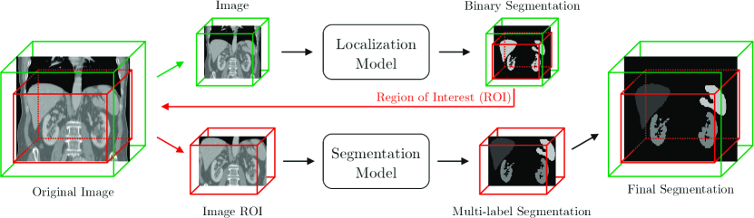
Figure 1: Schematic overview of our method. First, using the full image content in a low resolution, we apply a localization model to predict a coarse binary segmentation from which we extract the region of interest (ROI) for further use. Then, the ROI is extracted from the original image in a high resolution and used as the input of our segmentation model to predict the final multi-label segmentation. Lastly, the final segmentation is resampled to match the original image.

Motivated to improve the quality of the predictions for unseen images without using any additional data, we propose to use the Spatial Configuration Network (SCN), which was originally applied for landmark localization [8, 9] and later adapted to multi-label segmentation of the heart [10]. We hypothesize that the SCN, which consists of a local and spatial network, results in better predictions for unseen images as the spatial network integrates prior knowledge of the spatial configuration among the labelled organs which can be used to resolve spurious responses. Furthermore, we carefully modified the SCN to reduce model complexity as much as possible without drastically impacting the quality of the segmentation results by observing the tradeoff between efficiency and segmentation quality. Lastly, we optimized the code to generate predictions for unseen images by minimizing computation time as well as the required Graphics Processing Unit (GPU) memory.

2 Method

In this work, we propose a multi-organ segmentation approach, where first a localization model is used to determine the region of interest (ROI) before employing a segmentation model based on the SCN, see Fig. 1. Our code is available on GitHub.

2.1 Preprocessing

Localization of the Region of Interest

The utilized localization model receives the full volumetric image content as an input. As the intensity values of CT images are well defined by the Hounsfield scale, we do not perform an intensity normalization on a per image basis. However, we divide the intensity values of all our images by 2048 and clip them to $[-1,1]$. After performing a Gaussian smoothing with $\sigma=3$, we linearly resample the images to a spacing of $6\times 6\times 6$ mm and an image size between $32\times 32\times 32$ and $80\times 80\times 256$ depending on the physical resolution of the original image yielding $\mathbf{x}_{\text{loc}}$. In cases where the resampled images still would not fit the maximum image size, we increase the image spacing even more such that the resampled image will fit.

Table 1: Data split of FLARE 2021.

Data Split	Center	Phase	# Num.
Training ( 361 cases )	The National Institutes of Health Clinical Center	portal venous phase	80
	Memorial Sloan Kettering Cancer Center	portal venous phase	281
Validation ( 50 cases )	Memorial Sloan Kettering Cancer Center	portal venous phase	5
	University of Minnesota	late arterial phase	25
	7 Medical Centers	various phases	20
Testing ( 100 cases )	Memorial Sloan Kettering Cancer Center	portal venous phase	5
	University of Minnesota	late arterial phase	25
	7 Medical Centers	various phases	20
	Nanjing University	various phases	50

Multi-Organ Segmentation

Our segmentation model utilizes the ROI predicted by the localization model to reduce the memory footprint of the image by cropping it. This allows the content within the ROI to retain a larger resolution compared to the image used by our localization model. Consequently, all images are cropped to a size between $32\times 32\times 32$ and $160\times 128\times 160$ with a spacing of $2\times 2\times 2$ mm or larger, in case the ROI would exceed the maximum image size. To train our segmentation model, we computed the bounding box containing every labelled voxel directly from the ground truth for each training sample. During inference, where the ground truth label is not available, we used the ROI predicted by our localization model to retrieve the relevant region of the image. In both cases, we additionally increased the ROI by up to $16$ voxels in both directions of each dimension independently to also include some of the surrounding anatomy depending on the remaining size of the image towards the respective border, yielding the input of our segmentation model $\mathbf{x}_{\text{seg}}$. Again, the intensity values of each image were divided by 2048 and clipped to $[-1,1]$.

2.2 Proposed Method

Localization of the Region of Interest

Our localization model $\mathcal{M}_{\text{loc}}$ is implemented as a coarse binary segmentation CNN where all labelled organs are treated as the foreground label and which is trained using the full image content after greatly downsampling the image to reduce the memory footprint. First, the image $\mathbf{x}_{\text{loc}}$ is used as input for the localization model to predict a binary segmentation $\mathbf{\hat{y}}_{\text{loc}}=\mathcal{M}_{\text{loc}}(\mathbf{x}_{\text{loc}})$. The binary segmentation is then used to compute a bounding box containing every segmented voxel, which we define as the ROI. The network architecture of the localization model was adapted from the U-Net [7] and trained using a generalized dice loss [11], i.e.,

$$L_{\text{loc}}=L_{\text{GD}}(\mathbf{y}_{\text{loc}},\mathbf{\hat{y}}_{\text{loc}}),$$ (1)

where $\mathbf{y}_{\text{loc}}$ represents the ground truth label resampled to the same size and spacing as the image $\mathbf{x}_{\text{loc}}$. Our localization model uses in total 637,474 parameters and the total number of Floating Point Operations (FLOPS) for one forward pass ranges from 8,613,207,612 for input size $32\times 32\times 32$ to 430,660,377,660 for input size $80\times 80\times 256$.

Multi-Organ Segmentation

The proposed segmentation model $\mathcal{M}_{\text{seg}}$ uses the image $\mathbf{x}_{\text{seg}}$ as input and is trained to predict a multi-label segmentation $\mathbf{\hat{y}}_{\text{seg}}$, i.e., $\mathbf{\hat{y}}_{\text{seg}}=\mathcal{M}_{\text{seg}}(\mathbf{x}_{\text{seg}})$. The architecture of our segmentation model is based on the SCN, which was originally proposed for landmark localization [8, 9] and later adapted to multi-label segmentation of the whole heart [10]. In this work, we adapted the SCN to multi-organ segmentation and simultaneously reduced its memory footprint. To train the proposed architecture, we employed a supervised loss on the final prediction $\mathbf{\hat{y}}_{\text{seg}}$ of the segmentation model as well as on the intermediate prediction of the local and spatial network to ensure that both subnetworks lead to a plausible prediction on their own. Defining the input and output of the local network as $\mathbf{x}_{\text{seg}}^{1}$ and $\mathbf{\hat{y}}_{\text{seg}}^{1}$ and of the spatial network as $\mathbf{x}_{\text{seg}}^{2}$ and $\mathbf{\hat{y}}_{\text{seg}}^{2}$ allows formulate the loss function as:

$$L_{\text{seg}} =L_{\text{GD}}(\mathbf{y}_{\text{seg}},\mathbf{\hat{y}}_{\text{seg}})+\lambda_{\text{seg}}^{1}L_{\text{CE}}(\mathbf{y}_{\text{seg}},\mathbf{\hat{y}}_{\text{seg}}^{1})$$ (2)

$$+\lambda_{\text{seg}}^{2}L_{\text{CE}}(\mathbf{y}_{\text{seg}},\mathbf{\hat{y}}_{\text{seg}}^{2}),$$

where the ground truth $\mathbf{y}_{\text{seg}}$ was resampled identically to the image $\mathbf{x}_{\text{seg}}$. The terms $L_{\text{GD}}$ and $L_{\text{CE}}$ represent the generalized dice loss and cross-entropy loss functions respectively and $\lambda_{\text{seg}}^{1}$ and $\lambda_{\text{seg}}^{2}$ are hyperparameters used to weight the individual loss functions. Overall, our segmentation model uses 1,270,090 parameters and requires 8,797,627,020 FLOPS for an input size of $32\times 32\times 32$ and 879,762,672,300 FLOPS when using an input size of $160\times 128\times 160$.

2.3 Post-processing

We do not perform any post-processing other than resampling the final prediction to the same size, spacing, etc. as the original input.

3 Dataset and Evaluation Metrics

3.1 Dataset

The dataset used in the FLARE 2021 Challenge is adapted from MSD [12] (Liver [13], Spleen, Pancreas), NIH Pancreas [14, 15, 16], KiTS [17, 18], and Nanjing University under the license permission. For more detailed information on the dataset, please refer to the challenge website and [19].

In total, the dataset consists of 511 images. The dataset is split into a training, validation and test set containing approximately $70\%$, $10\%$ and $20\%$ respectively, resulting in 361 training cases, 50 validation cases, and 100 test cases. More detailed information is presented in Table 1.

3.2 Evaluation Metrics

In the evaluation, both accuracy and efficiency of the model will be considered to rank the challenge participants using the following metrics:

• Dice Similarity Coefficient (DSC)

• Normalized Surface Distance (NSD)

• Running time

• Maximum used GPU memory (when the inference is stable)

4 Implementation Details

4.1 Environments and requirements

We implemented our method in Python and used TensorFlow as a deep learning framework. SimpleITK was used to read and write the medical images as well as their meta-data to retrieve the image information as NumPy arrays. Detailed information on the environment used during the development of our method is given in Table 2.

Table 2: Environment and requirements.

Oberating System	Linux Manjaro 5.13.5-1
CPU	AMD Ryzen 9 3900X
RAM	16$\times$4GB
GPU	Nvidia GeForce 2080Ti
CUDA version	11.4
Programming language	Python 3.9
Deep learning framework	TensorFlow 2.6
Specification of dependencies	SimpleITK 2.0, NumPy 1.20, SciPy 1.7, scikit-image 0.18, tqdm 4.61

4.2 Training protocols

While the localization model is based on the U-Net [7] and the segmentation model on the SCN [10], the architecture of the localization model as well as the architectures of the local and spatial network of the segmentation model follow the same structure. Namely, each architecture consists of a sequence of contracting blocks that are followed by the same number of expanding blocks. Additionally, each contracting block is connected by a skip connection to the expanding block on the same level of depth, similar to the U-Net [7]. Each block consists of two consecutive convolution and dropout layers [20]. Furthermore, each convolution with the exception of the final one employs a kernel size of $3\times 3\times 3$ and leaky ReLU [21] with $\alpha=0.1$. The final convolution uses a linear function and the number of filters is set to the number of labels. The dropout ratio is set to 0.1 and we use average pooling and linear upsampling with a stride of $2\times 2\times 2$ as well as He initialization [21]. We use a mini-batch size of 1, employ Adam [22] as optimizer with a learning rate of 0.0001 and compute the model weights as an exponential moving average. Our localization model as well as the local network of our segmentation model use 5 levels of depth and 32 filters for intermediate convolution layers, while the spatial network of our segmentation model uses 4 levels of depth and 16 filters. Whenever a sample is selected during training, we perform data augmentation via a random transformation consisting of a translation, rotation, scale and elastic deformation, as well as an intensity shift and scale. See Table 3 for more details.

To develop our method and evaluate the performance of our segmentation model, we conducted a 4-fold cross-validation for which we split the 361 labelled images of the training set into 4 random folds. Each segmentation model in our cross-validation experiment was trained for 100,000 iterations. During our experiments, we observed that a model with reduced complexity is able to catch up to the performance of a more complex model when it is trained for more iterations. Thus, for our final submission, we increased the number of iterations to train the localization and segmentation model to 1,000,000 and 500,000 iterations respectively.

Table 3: Training protocols.

Data augmentation methods	Rotation, translation, scaling, elastic deformation, intensity shift and scaling
Initialization of the network	He normal initialization
Batch size	1
Patch sampling strategy $\mathcal{M}_{\text{loc}}$	full image
Patch size $\mathcal{M}_{\text{loc}}$	[$32\times 32\times 32$] to [$80\times 80\times 256$]
Image spacing $\mathcal{M}_{\text{loc}}$	$6\times 6\times 6$ mm
Total iterations $\mathcal{M}_{\text{loc}}$	1,000,000
Patch sampling strategy $\mathcal{M}_{\text{seg}}$	ROI from ground truth (training) or localization model (inference)
Patch size $\mathcal{M}_{\text{seg}}$	[$32\times 32\times 32$] to [$160\times 128\times 160$]
Image spacing $\mathcal{M}_{\text{seg}}$	$2\times 2\times 2$ mm
Total iterations $\mathcal{M}_{\text{seg}}$	500,000
Optimizer	Adam ($\beta_{1}=0.9$, $\beta_{2}=0.999$)
Initial learning rate	0.0001
Learning rate decay schedule	constant
Stopping criteria, and optimal model selection criteria	Stopping criterion is reaching the maximum number of iterations.
Training time $\mathcal{M}_{\text{loc}}$	11.0 hours
Training time $\mathcal{M}_{\text{seg}}$	49.0 hours
CO2eq $\mathcal{M}_{\text{loc}}$	1,183 g
CO2eq $\mathcal{M}_{\text{seg}}$	7,136 g

Table 4: Quantitative results of 4-fold cross-validation in terms of DSC and NSD.

Training	Liver		Kidney		Spleen		Pancreas
	DSC (%)	NSD (%)	DSC (%)	NSD (%)	DSC (%)	NSD (%)	DSC (%)	NSD (%)
Fold-1	$97.6\pm 2.1$	$88.4\pm 6.5$	$95.0\pm 3.1$	$85.2\pm 6.1$	$96.3\pm 10.5$	$94.5\pm 11.1$	$82.7\pm 8.7$	$62.7\pm 13.9$
Fold-2	$97.8\pm 1.1$	$88.9\pm 4.9$	$95.5\pm 1.7$	$86.0\pm 5.1$	$97.4\pm 1.4$	$95.5\pm 4.1$	$83.0\pm 6.1$	$61.5\pm 13.9$
Fold-3	$97.8\pm 0.9$	$89.0\pm 4.4$	$94.3\pm 6.3$	$84.8\pm 7.5$	$97.5\pm 2.3$	$95.6\pm 4.4$	$81.5\pm 9.4$	$59.8\pm 15.6$
Fold-4	$97.9\pm 0.7$	$89.2\pm 3.9$	$95.4\pm 2.7$	$86.2\pm 5.4$	$97.8\pm 0.6$	$96.2\pm 2.7$	$82.0\pm 9.5$	$59.3\pm 16.7$
Average	$97.8\pm 1.3$	$88.9\pm 5.0$	$95.0\pm 3.9$	$85.6\pm 6.1$	$97.2\pm 5.5$	$95.4\pm 6.5$	$82.3\pm 8.6$	$60.8\pm 15.1$

4.3 Testing protocols

To optimize inference time as well as the required GPU memory, we implemented a minimal script for inference. After loading an image, the same preprocessing strategy for the localization model as during training is performed before generating the models prediction from which the ROI is computed. Using the ROI, we also perform the same preprocessing strategy for the segmentation model as during training. Lastly, we resample the prediction of our segmentation model such that it has the same size and spacing as the original image and copy all of the meta-data, i.e., origin, direction, orientation, etc., from it as well.

5 Results

We evaluate our segmentation model on the 4-fold cross-validation quantitatively as well as qualitatively. Furthermore, we also observe the performance of our final submitted models on the hidden validation set, for which the organizers provided quantitative results as well as selected groundtruth images after the challenge deadline.

5.1 Quantitative Results of 4-fold Cross-Validation

The evaluation of our 4-fold cross-validation confirms good performance of our segmentation model for multi-label segmentation, see Table 4. The average Dice Score (DSC) of liver, kidney and spleen are $97.8\%$, $95.0\%$ and $97.2\%$, respectively, while the pancreas has the lowest DSC of $82.3\%$. In terms of Normalized Surface Distance (NSD), which is computed as the percentage of voxels for which the surface distance is below 1 mm, our method achieves a score of $88.9\%$, $85.6\%$ and $95.4\%$ for liver, kidney and spleen respectively. Again, the performance of the pancreas is lowest, resulting in a NSD of $60.8\%$.

5.2 Quantitative Results on Validation Set

Table 5 shows the performance of our submitted localization and segmentation model in terms of DSC and NSD on the hidden validation set. Similar to the cross-validation results, the segmentation of liver, kidney and spleen were better by a large margin compared to the pancreas. In terms of DSC, liver, kidney and spleen respectively achieved $95.43\%$, $89.74\%$ and $93.88\%$ on average, while the pancreas scored $75.15\%$. The spleen performed best in terms of NSD with $86.57\%$ followed by liver and kidney with $80.03\%$ and $77.76\%$ respectively. Lastly, the NSD of the pancreas achieved $60.00\%$ on average, meaning that $60.00\%$ of all voxels labelled as pancreas resulted in a surface distance below 1 mm.

Table 5: Quantitative results on validation set.

Organ	DSC (%)	NSD (%)
Liver	95.43 $\pm$ 4.77	80.03 $\pm$ 12.24
Kidney	89.74 $\pm$ 13.71	77.76 $\pm$ 15.89
Spleen	93.88 $\pm$ 14.02	86.57 $\pm$ 17.55
Pancreas	75.15 $\pm$ 18.52	60.00 $\pm$ 16.82

5.3 Qualitative Results

Selected qualitative results of our proposed model trained on the cross-validation are given in Fig. 2, while Fig. 3 shows results of our submitted model evaluated on the hidden validation set. In both Figures, the image, the ground truth label as well as the models prediction are shown from left to right. The segmented organs are the liver (red), the kidneys (green), the spleen (blue) and the pancreas (yellow). The image given in the first row in Fig. 2 and 3 represents a selected case, where the prediction of our model is very close to the ground truth for all labels. In rows 2-4 in Fig. 2, some of the most difficult cases from the cross-validation set are shown, for which we selected images with the lowest DSC. Similarly, rows 2-4 in Fig. 3 shows difficult cases of the validation set, which were selected by the challenge organizers.

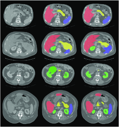
Figure 2: Qualitative results of our 4-fold cross-validation showing the image (column 1), the ground truth (column 2) and the prediction of our model. A case of a successful prediction is given in row 1, while rows 2-4 represent difficult cases selected according to their DSC.

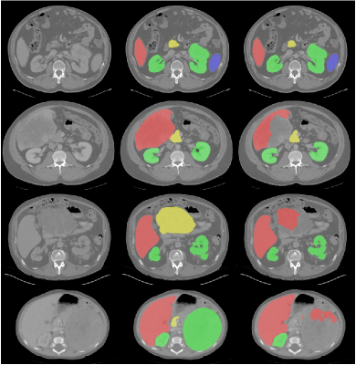
Figure 3: Qualitative results of our submitted segmentation model on the validation set showing the image (column 1), the ground truth (column 2) and the model prediction. A case of a successful prediction is given in row 1, while rows 2-4 represent difficult cases selected by the challenge organizers.

6 Discussion and Conclusion

Observation of the quantitative results in Table 4 shows, that the segmentation for liver, kidney and spleen perform very well with each achieving a DSC of at least $95\%$, while the segmentation of the pancreas only reached $82.3\%$ The results of the NSD show a similar trend, where again the segmentation of the pancreas performed worse by a large margin reaching only $60.8\%$, even though the segmentation of the liver and kidney achieved more than $85\%$ on average. The spleen showed the best results in NSD with $95.4\%$, which means that less than $5\%$ of all voxels labelled as spleen had a surface distance of more than 1 mm. The quantitative results of the submitted model on the validation set given in Table 5 follow the same trend with liver, kidney and spleen performing a lot better in terms of DSC and NSD on average compared to the pancreas. The segmentation of both, liver and spleen, achieved a DSC of over $90\%$ closely followed by the kidney with $89.74\%$, however, the pancreas only managed to reach a DSC of $75.15\%$. In terms of NSD, liver and spleen resulted in a score of over $80\%$ on the validation set, while the kidney reached $77.76\%$. Again, the pancreas in comparison to the other labels underperformed by a margin achieving $60.00\%$ measured in NSD.

When comparing the quantitative results of the cross-validation set in Table 4 to the results of the submitted model evaluated on the validation set in Table 5, it can be observed that both, DSC and NSD for all labels are lower on the validation set. This gap in performance is caused by the data used to train and evaluate the respective model, as the cross-validation models were trained and evaluated only on subsets of the training set, while the submitted model was trained on the full training set and evaluated on the validation set. As can be seen in Table 1, the training set only consists of images obtained from two centers with the same phase. In contrast, the validation set contains images from 9 different centers of which 8 have been unseen during training as well as images with various phases, including many samples with phases also unseen during training. Consequently, while the cross-validation set can be used to evaluate how well the model performs on the task, the evaluation on the validation set shows how well the model generalizes to data from different centers with various phases.

When observing the qualitative results of difficult cases of the cross-validation set in Fig. 2, rows 2-4, more closely, it becomes apparent that all three images are pathological and contain a rather large lesion which our model failed to label correctly. More precisely, the image in row 2 contains a large lesion of the pancreas (yellow) of which some parts were labelled correctly by our model, while other parts of the lesion where either not labelled or even mislabelled as the spleen (blue). In row 3, again a very large lesion of the kidney (green) on the left can be observed, which is completely missing in the prediction of our model. The image in the last row contains a lesion of the pancreas (yellow), which is also not labelled by our segmentation model. Nevertheless, when looking at row 1, the labels of the healthy organs in rows 2-4 as well as the healthy parts of the labels containing these huge lesions in rows 2-4, it can be observed that the predictions are very close to the ground truth labels. Similarly, the qualitative results of difficult cases of the validation set in Fig. 3 given in rows 2-4 contain very large lesions which were not labelled correctly by our model. In row 2, the liver (red) contains a large lesion spanning almost over the whole liver in this slice. The spleen (yellow) in row 3 as well as the right kidney (green) in row 4 of the presented slices are also lesions which lead to a huge inflation of the respective organ. All three of these huge lesions could not be labelled correctly by our segmentation model and in some cases even lead to our model mislabeling these regions. Nevertheless, healthy and less severe pathological organs were segmented very well including small and medium sized lesions as can be observed from the right kidney (green) in row 3, bottom, and again the right kidney in row 1, top.

A closer look at the dataset reveals that many of the organs per image are either healthy or only contain smaller lesions which are easier to learn and thus, more likely to be segmented correctly. In contrast, large lesions of individual organs are only present in a small number of images which can lead to lacking segmentation predictions for unseen images if this type of pathology was never or not sufficiently encountered during training. This indicates, that additional data containing very large lesions would be beneficial to solve the problems observed in these regions. Other potential solutions, which are not based on acquiring additional data, are to either use an imbalanced training scheme, where images with large lesions are selected more frequently during training, or a more sophisticated data augmentation strategy, where large lesions are injected artificially into the image using, e.g., a local inflation operation.

References

- [1] Z. Liao, J. J. Lee, R. Komaki, D. R. Gomez, M. S. O’Reilly, F. V. Fossella, G. R. Blumenschein Jr, J. V. Heymach, A. A. Vaporciyan, S. G. Swisher et al., “Bayesian Adaptive Randomization Trial of Passive Scattering Proton Therapy and Intensity-Modulated Photon Radiotherapy for Locally Advanced Non–Small-Cell Lung Cancer,” Journal of Clinical Oncology, vol. 36, no. 18, p. 1813, 2018.
- [2] A. Gotra, L. Sivakumaran, G. Chartrand, K.-N. Vu, F. Vandenbroucke-Menu, C. Kauffmann, S. Kadoury, B. Gallix, J. A. de Guise, and A. Tang, “Liver Segmentation: Indications, Techniques and Future Directions,” Insights into Imaging, vol. 8, no. 4, pp. 377–392, 2017.
- [3] A. Virzì, C. O. Muller, J.-B. Marret, E. Mille, L. Berteloot, D. Grévent, N. Boddaert, P. Gori, S. Sarnacki, and I. Bloch, “Comprehensive Review of 3D Segmentation Software Tools for MRI Usable for Pelvic Surgery Planning,” Journal of Digital Imaging, vol. 33, no. 1, pp. 99–110, 2020.
- [4] Y. Fu, Y. Lei, T. Wang, W. J. Curran, T. Liu, and X. Yang, “A Review of Deep Learning based Methods for Medical Image Multi-Organ Segmentation,” Physica Medica, vol. 85, pp. 107–122, 2021.
- [5] C. Chen, C. Qin, H. Qiu, G. Tarroni, J. Duan, W. Bai, and D. Rueckert, “Deep Learning for Cardiac Image Segmentation: A Review,” Frontiers in Cardiovascular Medicine, vol. 7, p. 25, 2020.
- [6] A. Tiwari, S. Srivastava, and M. Pant, “Brain Tumor Segmentation and Classification from Magnetic Resonance Images: Review of Selected Methods from 2014 to 2019,” Pattern Recognition Letters, vol. 131, pp. 244–260, 2020.
- [7] O. Ronneberger, P. Fischer, and T. Brox, “U-Net: Convolutional Networks for Biomedical Image Segmentation,” in International Conference on Medical Image Computing and Computer-Assisted Intervention, 2015, pp. 234–241.
- [8] C. Payer, D. Štern, H. Bischof, and M. Urschler, “Regressing Heatmaps for Multiple Landmark Localization Using CNNs,” in International Conference on Medical Image Computing and Computer-Assisted Intervention. Springer, 2016, pp. 230–238.
- [9] C. Payer, D. Štern, H. Bischof, and M. Urschler, “Integrating Spatial Configuration into Heatmap Regression based CNNs for Landmark Localization,” Medical Image Analysis, vol. 54, pp. 207–219, 2019.
- [10] C. Payer, D. Štern, H. Bischof, and M. Urschler, “Multi-label Whole Heart Segmentation using CNNs and Anatomical Label Configurations,” in International Workshop on Statistical Atlases and Computational Models of the Heart. Springer, 2017, pp. 190–198.
- [11] C. H. Sudre, W. Li, T. Vercauteren, S. Ourselin, and M. J. Cardoso, “Generalised Dice Overlap as a Deep Learning Loss Function for Highly Unbalanced Segmentations,” in Deep Learning in Medical Image Analysis and Multimodal Learning for Clinical Decision Support. Springer, 2017, pp. 240–248.
- [12] A. L. Simpson, M. Antonelli, S. Bakas, M. Bilello, K. Farahani, B. Van Ginneken, A. Kopp-Schneider, B. A. Landman, G. Litjens, B. Menze et al., “A Large Annotated Medical Image Dataset for the Development and Evaluation of Segmentation Algorithms,” arXiv preprint arXiv:1902.09063, 2019.
- [13] P. Bilic, P. F. Christ, E. Vorontsov, G. Chlebus, H. Chen, Q. Dou, C.-W. Fu, X. Han, P.-A. Heng, J. Hesser et al., “The Liver Tumor Segmentation Benchmark (LiTS),” arXiv preprint arXiv:1901.04056, 2019.
- [14] H. Roth, A. Farag, E. Turkbey, L. Lu, J. Liu, and R. Summers, “Data from Pancreas-CT. The Cancer Imaging Archive (2016).”
- [15] H. R. Roth, L. Lu, A. Farag, H.-C. Shin, J. Liu, E. B. Turkbey, and R. M. Summers, “DeepOrgan: Multi-level Deep Convolutional Networks for Automated Pancreas Segmentation,” in International Conference on Medical Image Computing and Computer-Assisted Intervention. Springer, 2015, pp. 556–564.
- [16] K. Clark, B. Vendt, K. Smith, J. Freymann, J. Kirby, P. Koppel, S. Moore, S. Phillips, D. Maffitt, M. Pringle et al., “The Cancer Imaging Archive (TCIA): Maintaining and Operating a Public Information Repository,” Journal of Digital Imaging, vol. 26, no. 6, pp. 1045–1057, 2013.
- [17] N. Heller, F. Isensee, K. H. Maier-Hein, X. Hou, C. Xie, F. Li, Y. Nan, G. Mu, Z. Lin, M. Han et al., “The State of the Art in Kidney and Kidney Tumor Segmentation in Contrast-Enhanced CT Imaging: Results of the KiTS19 Challenge,” Medical Image Analysis, vol. 67, p. 101821, 2021.
- [18] N. Heller, S. McSweeney, M. T. Peterson, S. Peterson, J. Rickman, B. Stai, R. Tejpaul, M. Oestreich, P. Blake, J. Rosenberg et al., “An International Challenge to use Artificial Intelligence to Define the State-of-the-Art in Kidney and Kidney Tumor Segmentation in CT Imaging.” American Society of Clinical Oncology, vol. 38, no. 6, pp. 626–626, 2020.
- [19] J. Ma, Y. Zhang, S. Gu, C. Zhu, C. Ge, Y. Zhang, X. An, C. Wang, Q. Wang, X. Liu, S. Cao, Q. Zhang, S. Liu, Y. Wang, Y. Li, J. He, and X. Yang, “AbdomenCT-1K: Is Abdominal Organ Segmentation A Solved Problem?” IEEE Transactions on Pattern Analysis and Machine Intelligence, 2021.
- [20] G. E. Hinton, N. Srivastava, A. Krizhevsky, I. Sutskever, and R. R. Salakhutdinov, “Improving Neural Networks by Preventing Co-Adaptation of Feature Detectors,” arXiv preprint arXiv:1207.0580, 2012.
- [21] K. He, X. Zhang, S. Ren, and J. Sun, “Delving Deep into Rectifiers: Surpassing Human-Level Performance on ImageNet Classification,” in Proceedings of the IEEE International Conference on Computer Vision, 2015, pp. 1026–1034.
- [22] D. P. Kingma and J. L. Ba, “Adam: A Method for Stochastic Optimization,” in Proceedings of the International Conference on Learning Representations, 2015.