Nucleon Charges and Sigma Terms from $N_{f}=2+1$ QCD

Abstract

We report on recent progress of our analysis of the nucleon sigma terms, as well as the singlet scalar, axial and tensor nucleon charges. These are determined employing the CLS gauge ensembles, which are generated using the Lüscher-Weisz gluon action and the non-perturbatively improved Sheikholeslami-Wohlert fermion action with $N_{f}=2+1$ dynamical fermions. For the ensembles analysed thus far, the pion masses range from 200 MeV up to 410 MeV, and the lattice spacings take five values between 0.09 fm and 0.04 fm. We have employed a variety of methods to determine the relevant correlation functions, including the sequential source method for connected contributions and the truncated solver method for disconnected contributions.

1 Introduction

The nucleon charges ($g^{q}_{X}$) are matrix elements of the form $\expectationvalue{J}{N}$, where the current $J=\overline{q}\Gamma q$ is composed of spinor fields of quark flavour $q\in\{u,d,s\}$ and $\Gamma\in\{\mathds{1},\gamma^{5}\gamma^{\mu},\gamma^{\mu},\frac{i}{2}[\gamma^{\mu}\gamma^{\nu}]\}$ for the scalar, axial, vector, and tensor charges ($X=S,A,V$ and $T$), respectively. Of particular note are the sigma terms which are obtained from the scalar charges through the multiplication with the mass of the quark $m_{q}$: $\sigma_{q}=m_{q}g_{S}^{q}=m_{q}\expectationvalue{\overline{q}\mathds{1}q}{N}$. These are of interest, for example, as they appear in the decomposition of the nucleon mass [1] (representing the quark contribution to the mass), and are required to predict the spin-independent WIMP-nucleon scattering cross section relevant for dark matter detection experiments. The axial charges give the contributions of the quark spins to the spin of the nucleon (as well as the coupling to the $Z$-boson), while the tensor charges correspond to the quark transverse spins in the nucleon.

2 Lattice Setup

We utilise the $N_{f}=2+1$ CLS ensembles [2] within our analysis, which were generated with the Lüscher-Weisz gluonic action, and the non-perturbatively improved Sheikholeslami-Wohlert fermionic action. There are several important aspects of this setup. We have $\mathcal{O}(a)$ non-perturbative improvement of the fermion action, however, the currents also require improvement, which, in general, involves both quark mass dependent and independent terms. As we are working in the forward limit, the latter do not appear (as they involve derivatives). The only exception to this is the scalar current, for which the mass-independent improvement term is proportional to $aFF$. We omit this term as the corresponding coefficient has not yet been determined. For this preliminary analysis, the mass-dependent terms are also not considered (for all of the charges). Note that, due to chiral symmetry breaking, there can be mixing between quark flavours under renormalisation. This is discussed in section 4.

The light and strange quark masses are varied in the simulation so as to follow three trajectories. As shown in figure 1, two of the trajectories approach the physical point (one along which the flavour average quark mass is held constant and the other along which the physical strange quark mass is kept approximately constant), while the other approaches the chiral limit. This allows for full control of quark-mass systematics. Furthermore, the range of lattice spacings (spanning 0.09 fm down to 0.04 fm) and volumes (with $L^{3}\cdot T=24^{3}\cdot 48$ up to $96^{3}\cdot 192$, with $Lm_{\pi}\gtrsim 4$ in almost all cases) available enables discretisation and finite volume effects to be thoroughly investigated. A high statistics study can be realised, with each ensemble typically containing around 1000–2000 configurations. Note that, in order to counter-act topological freezing, many ensembles (in particular, those at finer lattice spacing) have open boundary conditions in the time direction.

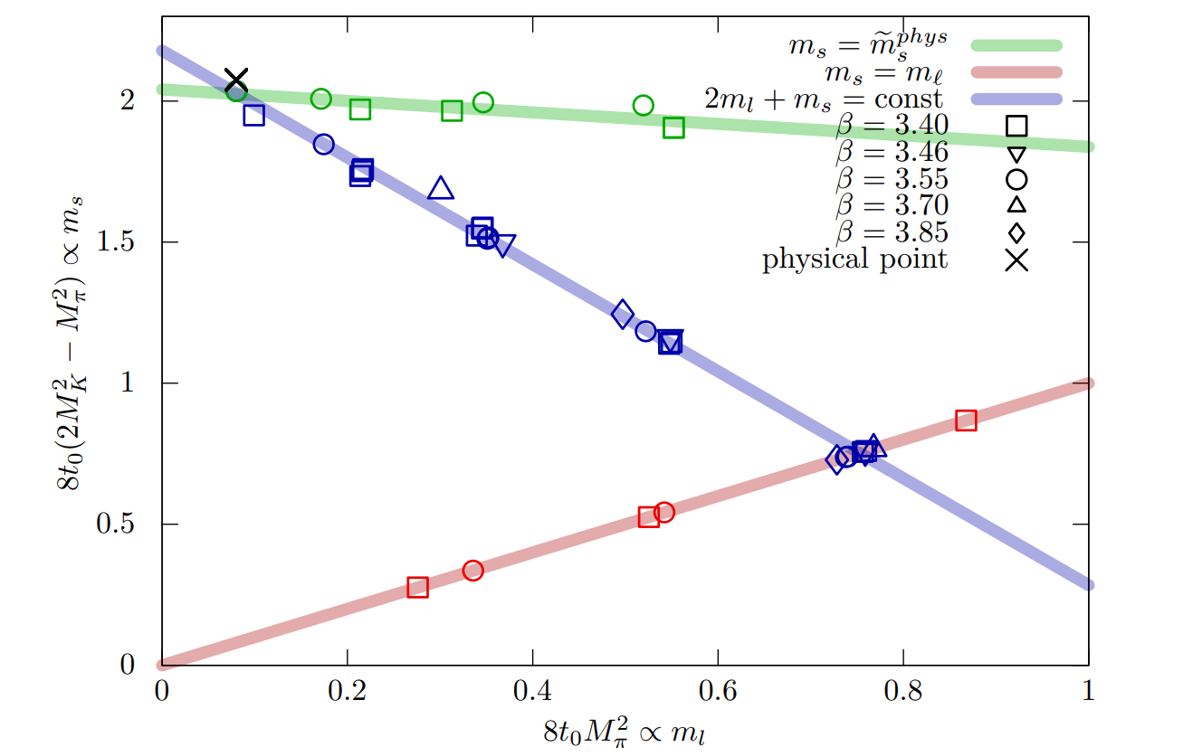
Figure 1: Overview of the CLS ensembles utilised within this analysis.

3 Correlation Functions

The correlation functions used are the standard two- and three-point functions

$$C_{2pt}(t_{f},t_{i})=\expectationvalue{\mathcal{N}(t_{f})\overline{\mathcal{N}}(t_{i})},$$ (1)

$$C_{3pt}(t_{f},t,t_{i})=\expectationvalue{\mathcal{N}(t_{f})J(t)\overline{\mathcal{N}}(t_{i})}-\expectationvalue{J(t)}\expectationvalue{\mathcal{N}(t_{f})\overline{\mathcal{N}}(t_{i})},$$ (2)

where $\overline{\mathcal{N}}$ ($\mathcal{N}$) is the nucleon interpolating operator at the source (sink) timeslice $t_{i}$ ($t_{f}$), and $J(t)=\overline{q}\Gamma q$ is the current inserted at time $t$ with spin structure $\Gamma$. We note the vacuum subtraction in equation 2 which is needed in the case of the scalar charge.

Performing the Wick contractions for the three-point correlation functions in equation 2 leads to quark line connected and disconnected diagrams. The connected contributions are generated through the use of the sequential source method. The source-sink separation for each three-point function is fixed and we realise four separations ranging from $t_{f}-t_{i}=0.7$ fm up to 1.2 fm. In order to improve statistics, multiple sources are analysed per configuration with one, two, three and four measurements being generated for the four separations ranging from the smallest to the largest. For the ensembles with periodic boundary conditions in time we make use of the coherent source technique [3].

The disconnected contributions are constructed by correlating a disconnected loop with a two-point function. For the two-point function, typically twenty different source positions are utilised. The calculation of the loop is computationally expensive, as this requires an all-to-all propagator. To offset this expense we make use of various techniques: the truncated solver method [4] together with the hopping parameter expansion [5] and partitioning [6] in the time direction. For the time partitioning we seed the stochastic source on every fourth timeslice, and then repeat this four times shifting the source by one timeslice each time.

The correlation functions are smeared at the source and the sink using Wuppertal smearing with APE smeared gauge links. The number of Wuppertal smearing iterations is varied with the pion mass such that the root-mean-square radius ranges between 0.6 fm and 0.85 fm as the pion mass decreases from 420 MeV down to the physical point. For ensembles with open boundary conditions, the positions of the nucleon source and sink are chosen such that boundary effects are avoided.

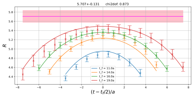
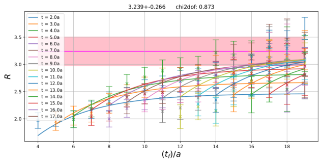
Figure 2: (Top) $R(t_{f},t)$ for a connected three-point function with a scalar current $J=\overline{u}\mathds{1}u$ as a function of the current insertion time for an ensemble with $m_{\pi}=345$ MeV, $a=0.0642$ fm, and $L^{3}\cdot T=3.08^{3}\cdot 8.22$ fm⁴, for four different source-sink separations in the range $t_{f}-t_{i}=0.7$ fm to $1.2$ fm. (Bottom) the ratio for a disconnected three-point function with $J=\overline{u}\mathds{1}u$ for multiple current insertion times as a function of the sink time. The connected and disconnected ratios relevant for extracting scalar, axial, tensor and vector charges are fitted simultaneously, with the pink bands indicating the ground state matrix elements extracted for the two ratios displayed.

3.1 Fitting

The spectral decompositions of the two- and three-point correlation functions, in the limit of large times, read

$$C_{2pt}(t_{f},0)=Z_{1}^{2}\textrm{e}^{-t_{f}m}\left[1+\frac{Z_{2}^{2}}{Z_{1}^{2}}\textrm{e}^{-\Delta mt_{f}}\right]+\ldots,$$ (3)

$$C_{3pt}(t_{f},t,0)=Z_{1}^{2}\textrm{e}^{-t_{f}m}\left[\expectationvalue{J}{1}+\frac{Z_{2}Z_{1}}{Z_{1}^{2}}\matrixelement{2}{J}{1}\left(\textrm{e}^{-\Delta m(t_{f}-t)}+\textrm{e}^{-\Delta mt}\right)\right]+\ldots,$$ (4)

where the overlap factors $Z_{j}\propto\matrixelement{0}{\mathcal{N}}{j}=Z_{j}^{*}$, and $\ket{0}$, $\ket{1}$ and $\ket{2}$ are the vacuum and the nucleon ground and first excited states, respectively. The mass gap between the first excited state and the ground state is denoted $\Delta m$. We fit the ratio of the two- and three-point correlation functions:

$$R(t_{f},t)=\frac{C_{3pt}(t_{f},t,0)}{C_{2pt}(t_{f},0)}=\expectationvalue{J}{1}+A\matrixelement{2}{J}{1}\left(\textrm{e}^{-\Delta m(t_{f}-t)}+\textrm{e}^{-\Delta mt}\right)+\ldots,$$ (5)

where the leading constant is the desired matrix element and any dependence on $t_{f}$ and $t$ is due to excited state contamination (only the leading correction is shown above), which can be significant. The excited state spectrum includes multi-particle states as well as radial excitations. In particular, for ensembles with lighter pion masses, the $N(0)\pi(0)\pi(0)$ or $N(\vec{p})\pi(-\vec{p})$ levels lie below that of the nucleon’s first radial excitation. Furthermore, as the pion mass approaches the physical point, the excited state spectrum becomes denser which may lead to difficulties in resolving individual excited state contributions.

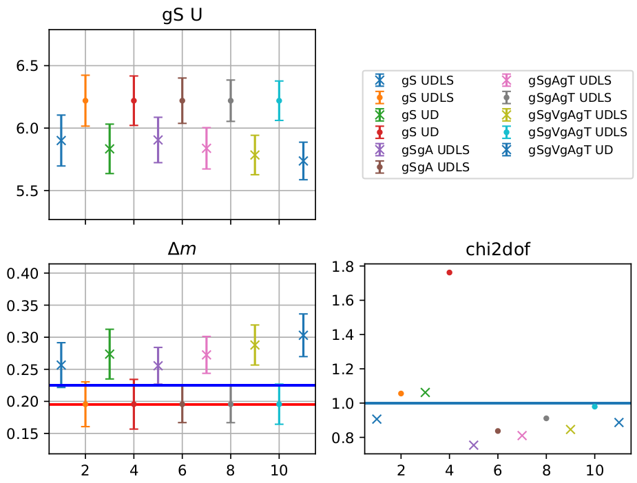
Figure 3: (Top left) bare connected scalar matrix element for $J=\overline{u}\mathds{1}u$ extracted when simultaneously fitting to different connected and disconnected three-point functions. The legend (top right) indicates which three-point functions (relevant for a particular charge) were included, with $U$ and $D$ ($L$ and $S$) indicating that connected (disconnected) three-point functions were fitted, with $J=\overline{u}\mathds{1}u$ and $\overline{d}\mathds{1}d$ ($J=\overline{u}\mathds{1}u=\overline{d}\mathds{1}d$ and $\overline{s}\mathds{1}s$), respectively. The crosses indicate fits where $\Delta m$ is a free parameter, while the points correspond to fits where the first excited state mass gap is set to the lowest non-interacting $p$-wave $N\pi$ energy using a prior. (Bottom left) The first excited mass gap extracted. The lowest non-interacting $p$-wave $N\pi$ ($s$-wave $N\pi\pi$) energy is shown as the red (blue) horizontal line. (Bottom right) The corresponding $\chi^{2}/$d.o.f. values.

In principle, the mass gap $\Delta m$ can be determined from a fit to the two-point function, however, as the overlap of the standard smeared nucleon interpolator with a $N\pi$ or $N\pi\pi$ state is small, it is often difficult to resolve the lowest excitation. In terms of the three-point function, the contribution of this level may be significant due to an enhanced $\matrixelement{2}{J}{1}$ matrix element. Alternatively, one can determine the mass gap when fitting to the ratio $R(t_{f},t)$, although, this can be problematic if the excited state contamination is small. In order to mitigate these difficulties, we perform a simultaneous fit to the connected and disconnected three-point functions corresponding to multiple charges, enforcing the same first excited state energy in each case. An example of such a fit is shown in figure 2, where, for brevity, only the ratios for a scalar current insertion $J=\overline{u}\mathds{1}u$ are displayed.

To check the assumption that the different charges have the same dominant excited state, we varied the three-point functions that enter the fit, as displayed in figure 3. To further investigate the sensitivity to the first excited state mass gap, we also performed fits where $\Delta m$ is set to the lowest non-interacting $p$-wave $N\pi$ energy using a prior. Figure 3 shows that the matrix element and mass gap are stable as we vary the three-point functions that are included in the fit. However, there is a systematic difference between the results with and without the prior which warrants further study.

4 Renormalisation

Matrix elements determined on the lattice are converted to the (standard) $\overline{\text{MS}}$ continuum scheme via renormalisation factors. When employing Wilson fermions, the flavour singlet and non-singlet renormalisation factors ($Z^{s}$ and $Z^{ns}$, respectively), in general, differ, due to the breaking of chiral symmetry. This leads to mixing between quark flavours under renormalisation. In perturbation theory, the ratio $r=Z^{s}/Z^{ns}=1+\mathcal{O}(\alpha^{n})$, where $r\to 1$ in the continuum limit (except in the case of the axial current due to the anomaly). For the axial and tensor charges, $n=2$ and $n=3$, respectively, suggesting the deviation from one is small. This seems to be confirmed by non-perturbative determinations of the ratios, see, e.g., [7].

For the scalar, while $Z^{s}/Z^{ns}=1+\alpha^{2}$, the ratio is known to be much larger than one for coarse lattice spacings. Considering the sigma terms, $\sigma_{q}=m_{q}g_{S}^{q}$, we start with the renormalisation pattern of the quark masses [8],

$$\begin{pmatrix}m_{u}(\mu)\\ m_{d}(\mu)\\ m_{s}(\mu)\end{pmatrix}^{\textrm{ren}}=Z^{ns}_{m}(\mu,a)\begin{pmatrix}\frac{r_{m}+2}{3}&\frac{r_{m}-1}{3}&\frac{r_{m}-1}{3}\\ \frac{r_{m}-1}{3}&\frac{r_{m}+2}{3}&\frac{r_{m}-1}{3}\\ \frac{r_{m}-1}{3}&\frac{r_{m}-1}{3}&\frac{r_{m}+2}{3}\end{pmatrix}\begin{pmatrix}m_{u}\\ m_{d}\\ m_{s}\end{pmatrix}^{\textrm{lat}},$$ (6)

where $r_{m}=Z^{s}_{m}/Z^{ns}_{m}$. Defining $\Tr M=\sum_{q}m_{q}$, $\Tr g_{S}=\sum_{q}g^{q}_{S}$, and $\widehat{\mathbb{O}}$ to be the renormalised observable $\mathbb{O}$, we can write

$$\widehat{m}_{q}=Z_{m}\left(m_{q}+\frac{r_{m}-1}{3}\Tr M\right),\qquad\widehat{g}^{q}_{S}=Z_{m}^{-1}\left(g^{q}_{S}+\frac{r_{m}^{-1}-1}{3}\Tr g_{S}\right)$$ (7)

which gives for the sigma terms

$$\sigma_{q}=\left(m_{q}+\frac{r_{m}-1}{3}\Tr M\right)\left(g^{q}_{S}+\frac{r_{m}^{-1}-1}{3}\Tr g_{S}\right).$$ (8)

Two flavour combinations of note are the pion-nucleon sigma term $\sigma_{N\pi}=\sigma_{u}+\sigma_{d}$ and the flavour singlet sigma term $\Tr\sigma=\sum_{q}\sigma_{q}$, which is invariant under renormalisation.

5 Preliminary Results

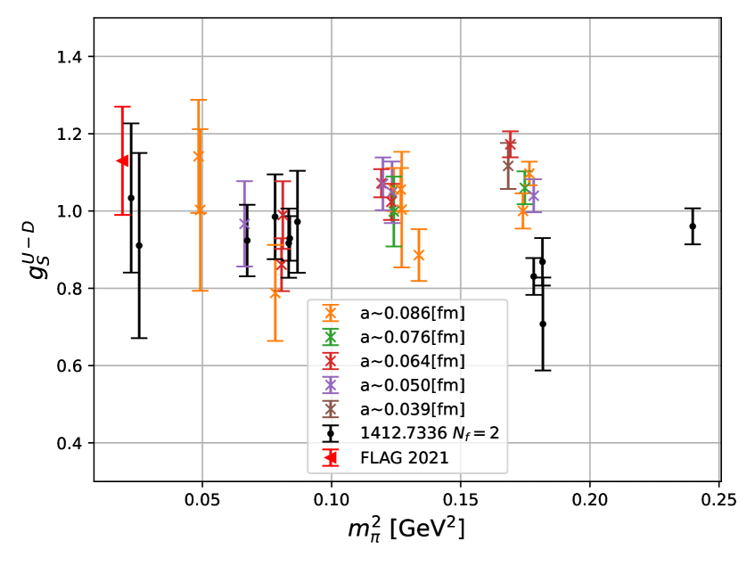
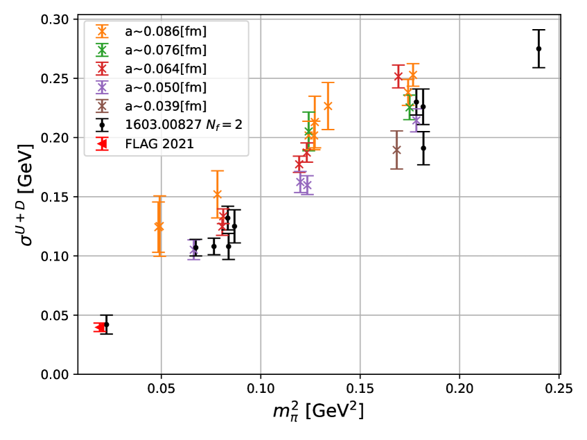
Figure 4: Preliminary results for the isovector scalar charge (left) and pion-nucleon sigma terms (right) determined on CLS $N_{f}=2+1$ ensembles compared to previous RQCD $N_{f}=2$ results [9] and the recent FLAG average [10].

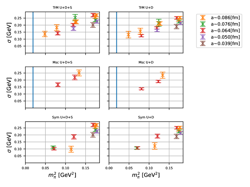
Figure 5: Dependence of the sigma terms on the pion mass squared for the singlet $\sigma_{u}+\sigma_{d}+\sigma_{s}$ flavour combination (left) and the pion-nucleon sigma term (right). The results for the three quark mass trajectories are given separately: (top) the ensembles lie on the trajectory along which the flavour average quark mass is kept constant, (middle) the strange quark mass is approximately constant, (bottom) the light and strange quark masses are equal. Where applicable, the vertical blue line indicates the physical pion mass.

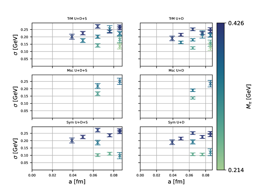
Figure 6: Dependence of the sigma terms on the lattice spacing for the singlet $\sigma_{u}+\sigma_{d}+\sigma_{s}$ flavour combination (left) and the pion-nucleon sigma term (right). The results for the three quark mass trajectories are given separately, as in figure 5. The pion mass in each case is indicated by a colour gradient.

In figure 4 we show preliminary results for the isovector scalar charge $g_{S}^{u-d}=g_{S}^{u}-g_{S}^{d}$ (left) and the pion-nucleon sigma term (right) determined on the $N_{f}=2+1$ ensembles which lie along the two trajectories that meet at the physical point as a function of the pion mass squared. Previous $N_{f}=2$ results from RQCD [9] are also shown for comparison, along with the recent $N_{f}=2+1$ FLAG average [11]. Note that results obtained on ensembles which lie along the trajectory, where the flavour average quark mass is kept fixed (the blue line of figure 1) are only expected to be consistent with the $N_{f}=2$ results close to the physical point. In figures 5 and 6 we present the pion mass and lattice spacing dependence of the results, respectively, for the three different trajectories separately. The downward trend in the data as the lattice spacing decreases suggests that there may be significant discretisation effects. In the future we will include further CLS ensembles and perform a combined continuum, quark mass and infinite volume extrapolation.

Acknowledgments. The authors were supported by the European Union’s Horizon 2020 research and innovation programme under the Marie Skłodowska-Curie grant agreement no. 813942 (ITN EuroPLEx) and grant agreement no 824093 (STRONG-2020) and by the Deutsche Forschungsgemeinschaft (SFB/TRR-55). The ensembles were generated as part of the CLS effort using OpenQCD [12], and further analysis was performed using a modified version of CHROMA [13], the IDFLS solver [14] and a multigrid solver [15]. The authors gratefully acknowledge the Gauss Centre for Supercomputing (GCS) for providing computing time through the John von Neumann Institute for Computing (NIC) on JUWELS [16] and on JURECA-Booster [17] at Jülich Supercomputing Centre (JSC). Part of the analysis was performed on the QPACE 3 system of SFB/TRR-55 and the Athene cluster of the University of Regensburg.

References

- [1] X. Ji et al., Qcd analysis of the mass structure of the nucleon, Physical Review Letters 74 (1995) 1071–1074.
- [2] M. Bruno et al., Simulation of qcd with flavors of non-perturbatively improved wilson fermions, Journal of High Energy Physics 2015 (2015) .
- [3] J.D. Bratt et al., Nucleon structure from mixed action calculations using2+1flavors of asqtad sea and domain wall valence fermions, Physical Review D 82 (2010) .
- [4] G.S. Bali et al., Effective noise reduction techniques for disconnected loops in lattice qcd, Computer Physics Communications 181 (2010) 1570–1583.
- [5] C. Thron et al., Padé estimator of determinants, Physical Review D 57 (1998) 1642–1653.
- [6] S. Bernardson et al., Monte Carlo methods for estimating linear combinations of inverse matrix entries in lattice QCD, Comput. Phys. Commun. 78 (1993) 256.
- [7] G.S. Bali et al., Non-perturbative renormalization of flavor singlet quark bilinear operators in lattice QCD, PoS LATTICE2016 (2016) 187 [1703.03745].
- [8] QCDSF collaboration, The strange and light quark contributions to the nucleon mass from Lattice QCD, Phys. Rev. D 85 (2012) 054502 [1111.1600].
- [9] RQCD collaboration, Direct determinations of the nucleon and pion terms at nearly physical quark masses, Phys. Rev. D 93 (2016) 094504 [1603.00827].
- [10] Flavour Lattice Averaging Group collaboration, FLAG Review 2019: Flavour Lattice Averaging Group (FLAG), Eur. Phys. J. C 80 (2020) 113 [1902.08191].
- [11] S. Aoki et al., FLAG review 2019, The European Physical Journal C 80 (2020) 113.
- [12] M. Lüscher and S. Schaefer, Lattice QCD with open boundary conditions and twisted-mass reweighting, Comput. Phys. Commun. 184 (2013) 519 [1206.2809].
- [13] SciDAC, LHPC, UKQCD collaboration, The Chroma software system for lattice QCD, Nucl. Phys. B Proc. Suppl. 140 (2005) 832 [hep-lat/0409003].
- [14] M. Lüscher et al., Deflation acceleration of lattice qcd simulations, Journal of High Energy Physics 2007 (2007) 011–011.
- [15] A. Frommer et al., Adaptive Aggregation Based Domain Decomposition Multigrid for the Lattice Wilson Dirac Operator, SIAM J. Sci. Comput. 36 (2014) A1581 [1303.1377].
- [16] Jülich Supercomputing Centre, JUWELS: Modular tier-0/1 supercomputer at the Jülich Supercomputing Centre, Journal of large-scale research facilities 5 (2018) .
- [17] Jülich Supercomputing Centre, JURECA: Modular supercomputer at Jülich Supercomputing Centre, Journal of large-scale research facilities 4 (2018) .