A Learned–SVD approach for Regularization in Diffuse Optical Tomography

Abstract

Diffuse Optical Tomography (DOT) is an emerging technology in medical imaging which employs light in the NIR spectrum to estimate the distribution of optical coefficients in biological tissues for diagnostic and monitoring purposes. DOT reconstruction implies the solution of a severely ill–posed inverse problem, for which regularization techniques are mandatory in order to achieve reasonable results. Traditionally, regularization techniques put a variance prior on the desired solution/gradient via regularization parameters, whose choice requires a fine tuning, specific for each case. In this work we explore deep learning techniques in a fully data–driven approach, able of reconstructing the generating signal (optical absorption coefficient) in an automated way. We base our approach on the so-called Learned Singular Value Decomposition, which has been proposed for general inverse problems, and we tailor it to the DOT application. We perform tests with increasing levels of noise on the measure, and compare it with standard variational approaches.

I Introduction

Diffuse Optical Tomography (DOT) is an emerging technology which employs light in the NIR spectral window to investigate biological tissues for diagnostic and monitoring purposes. Its use has been explored in different medical fields, including imaging of brain, thyroid, prostate, breast cancer screening and, more in general, for detecting and monitoring body functional changes related to blood flow [1, 2, 3]. Tomographic reconstruction in DOT aims at recovering the spatial distribution of tissue optical properties of the investigated organ, which can be related to chromophores concentration (mainly water, oxy and deoxy-hemoglobin and, in the case of adipose tissue as breast, lipids) for functional evaluation. To do this, light emitted from external sources at different positions is let to propagate throughout the investigated organ and the emerging photon flux is measured on the tissue boundary [4]. DOT reconstruction is a notoriously severely ill-posed and ill-conditioned inverse problem since at NIR wavelengths the outgoing light consists of a mixture of very few coherent and quasi–coherent photons and a predominant component of incoherent (diffusive) photons which experienced multiple scattering events. As such, the DOT technology is intrinsically sensitive to measurement noise and model errors.

Model-based image reconstruction algorithms (also known as variational approaches) have represented in the past the standard approach to perform DOT reconstruction (inverse problem). They usually consist of three components [1]:

1. a forward mathematical model that provides a prediction of the measurements based on a guess of the system parameters (the optical coefficients: the absorption coefficient $\mu_{a}$ [cm^-1] and the scattering coefficient $\mu_{s}$ [cm^-1]);

2. an objective functional that compares the predicted data with the measured data;

3. an efficient way of updating the system parameters of the forward model, which in turn provides a new set of predicted data.

This latter point has been approached both by linearization via the Born or Rytov approximations [5] and by nonlinear iterations formulated as optimization problems [6]. Due to the ill-conditioned nature of the reconstruction problem, all these approaches include a form of regularization, which provides hard or soft prior information on the solution. As for this latter category, the $\ell_{2}$–norm (Tikhonov/ridge regression) penalization is the benchmark classic regularization approach and has been widely used in DOT literature [7, 8, 9]. The $\ell_{1}$-norm (lasso) penalization has been mainly used in this context to improve sharp edges detection, obtained as a by–product of sparsity enhancement [10]. Some of the authors of the present paper proposed in [11, 12] the use of an Elastic–Net regularization term. This approach was investigated both in 2D and 3D domains under the Rytov approximation and provided results superior to the use of pure $\ell_{2}$ or $\ell_{1}$ strategies, the combination of which being able to give a satisfactorily stable solution with a preserved sparsity pattern. An alternative approach was proposed in [13], based on Bregman iterations [14]: this iterative technique consists in substituting the regularization function with its Bregman distance from the previous iterate. It has been proved [15] that this procedure provides a solution to the optimization problem and moreover it possess a remarkable contrast enhancement ability [16, 17], confirmed also in DOT framework [13]. Other regularization functionals have also been explored, among which we cite here the combined use of a TV method with $\ell_{1}$–norm in the TOAST++ software for DOT reconstruction [18]. All these approaches are far from being flawless: poor reconstruction results are common outcomes already in mildly complex situations and/or the reconstruction requires a very heavy computational time. Specifically, a main critical point is the fine tuning of regularization parameters required to obtain a reasonable solution. These parameters were observed to be strongly dependent on the geometry, mesh-size, optical coefficients distribution and level of noise of each single case, so that a general, effective, strategy cannot be obtained.

Recently, the outstanding performance on computer vision tasks of deep learning (DL) algorithms based on Neural Networks (NNs), and especially Convolutionary Neural Networks (CNNs), has motivated studies to explore their use also in DOT reconstruction, with the aim to overcome the above discussed weaknesses. The application of DL techniques to DOT problems is still at its beginnings and very recent: in [19] a Regularization by Denoising (RED) approach was proposed, while [20] trained a NN for inverting in an end–to-end fashion the Lippman–Scwhinger equation, by firstly learning the pseudoinverse of the nonlinear mathematical operator modelling the DOT physics, and then applying an encoder–autoencoder network to remove the remaining artifacts. In [21], the authors combined DL with a model-based approach using Gauss–Newton iterations where the update function was learned via a CNN. We refer to [22] for a review of the other few applications of DL in DOT reconstruction. In this work, we investigate and adapt to DOT reconstruction the general strategy for inverse problems of [23], called Learned–SVD. This approach consists in mapping measured data and generating signal into feature spaces and bridge them via a “singular value operator“ which acts as a learned regularization, and alleviates from the burden of a–priori choosing the regularization. The idea of learning the regularization via NNs is not new in the general field of inverse problem solution: for example, in [24] a regularization term was learned using only unsupervised data; in [25, 26] a Total Deep Variation functional was learned, while the NETT framework of [27] employs as regularizer the encoder part of an encoder–decoder NN. However, at the best of our knowledge, none of these approaches -including the present Learned-SVD- has been applied to DOT reconstruction.

We examined the performance of the Learned-SVD and compared it to classic variational approaches. According to the measured metrics, the present NN-based strategy performs significantly better and increasing levels of noise on the data have a reduced impact than on variational methods.

This paper is organized as follows. Section II presents the abstract mathematical setting of the DOT reconstruction problem; Section III presents the classic variational approaches, with specific focus on the Rytov linearization strategy; Section IV presents the Learned-SVD strategy with its connection to the SVD decomposition and Tikhonov regularization; Section V presents the results obtained with the proposed approach together with a comparison with standard variational reconstruction approaches; Section VI draws the conclusions.

II General setting

The goal of the DOT reconstruction is to map measured light data collected on the investigated tissue boundary into accurate approximate spatial distribution of the optical coefficients inside the tissue itself. Due to relevant aspects, which directly impact on the mathematical reconstruction problem, in this paper we focus on DOT based on continuous waves (CW) systems, which are among the most widely used in clinical settings for breast cancer screening, object of our past and present research work. In these systems, which are typically embedded in low-to-mid cost range hardware, the light source continuously emits light into the tissue at a single frequency and the measured data are light fluence outgoing from the tissue boundary. A minimal CW–DOT setting consists thus in an array of $n_{s}$ pointwise light sources located at positions ${\bm{s}}$ and emitting light at NIR wavelength into the tissue and a set of $n_{d}$ measures of the outgoing light flux. These latter can be collected by detectors physically located on the tissue surface at positions ${\bm{d}}$ or by a charge–coupled device (CCD) camera which produces (indirect) measures of the outgoing light intensity via grey-levels in an image. Additional elaborations are usually performed on the raw measures in order to (at least partially) filter out noise, eliminate under- and over-saturated pixels by thresholding procedures and define an appropriate ROI. We do not enter into details of these procedure, referring to [28] for an overview of the implicated workflow.

Let $q\in Q$ denote the set of spatially dependent optical properties of the tissue, $u\in V$ the intensity (or fluence) of the light in the tissue, and let $f=f({{\bm{s}}})\in W$ be a given source located at position ${{\bm{s}}}$, where $Q,V$ and $W$ are the Banach spaces of all admissible optical properties, light field and source terms, respectively. The set of parameters $q$ along with the given sources $f$ determine observations of quantities related to the variable state $u$ that are collected at the detector locations ${\bm{d}}$ as

$$y=\mathcal{M}(q,u;f),$$ (1)

where $y=[y({\bm{d}}_{1},{\bm{s}}_{1}),\dots,y({\bm{d}}_{n_{d}},{\bm{s}}_{n_{s}})],$ is the measurement vector and where $\mathcal{M}:(Q\times V\times W)\rightarrow Y$ is a bounded linear functional, $Y$ being a Banach data space. The operator $\mathcal{M}$ is a general representation of the measurement. Notice that measured data are invariably affected by noise, mainly electronic noise due to the detector acquisition chain but also from other artifacts like (in realistic conditions) patient’s movements and ambient light.

On the other side, we introduce the parameter-to-state map $\mathcal{F}:\Theta\rightarrow Y$ such that

$$\mathcal{F}(\theta)=\mathcal{P}u.$$ (2)

where $\theta$ is a set of parameters that will be specified below. One can pursue an approximation of $\mathcal{F}$ via a traditional (physics-driven, see Sect. Section III) or machine learning–based (data–driven, see Sect. Section IV) approach. In the first case, $\Theta\equiv Q$ and the parameter–to–state map arises from an underlying mathematical model, which, in the DOT context, describes light propagation in a biological tissue. Such a model can be represented in an abstract manner as

$$\mathcal{A}(q,u)=f,$$ (3)

where $\mathcal{A}:(Q\times V)\rightarrow W$ and if $u$ is a solution to (3) for a given $q$ and given source $f=f({\bm{s}})$ then $\mathcal{P}u$ is the trace of the solution and it is a quantity directly comparable to the datum $y$ in (1). On the other hand, when considering data–driven approaches, one does not dispose of an explicit model as in (3), but directly learns $\mathcal{F}$ from data, that is learning the set of parameters $\Theta$ (weights of the net). In both cases, to close the problem one must introduce a non–negative function, called discrepancy or loss function, $\mathcal{D}:\Theta\times Y\rightarrow\mathbb{R}^{+}$ that - considering the case of least squares - can be written as

$$\mathcal{D}(\theta;y)=\frac{1}{2}\|\mathcal{F}(\theta)-y\|_{Y}^{2}$$ (4)

and the DOT reconstruction problem is then formulated as

$$\begin{array}[]{l}{\theta}^{*}=\displaystyle\operatorname*{argmin}_{\theta\in\Theta}\mathcal{D}(\theta;y).\end{array}$$ (5)

III Variational approaches for DOT reconstruction

III-A Mathematical models of light propagation

As anticipated in the previous section, classic variational approaches in DOT reconstruction rely on the existence of a mathematical model. In this case, one disposes of an operator $\mathcal{A}(\cdot,\cdot)$ in (3) which is typically a differential law augmented by appropriate boundary conditions describing light propagation in scattering media. A physically reasonable and cost–effective model of this kind is derived by performing an expansion of the Radiative Transfer Equation (RTE) in spherical harmonics (see e.g. [29] for details and derivation). The following diffusion equation (DE) model is then obtained in steady state:

$$-\nabla\cdot(D({\bm{r}})\nabla u({\bm{r}}))+\mu_{a}({\bm{r}})u({\bm{r}})=f({\bm{s}}),$$ (6)

where ${\bm{r}}$ is the position [cm] in the connected open domain $\Omega\subset\mathbb{R}^{d},d=2$ or $3$, representing the tissue to be investigated (for example the breast), with outward unit normal vector ${{\bm{n}}}$. In (6), $u=u({\bm{r}})$ represents photon fluence [W/cm²] due to the light source $f=S_{0}\delta({\bm{r}}-{\bm{s}})$ [W/cm³], $S_{0}$ being the source intensity. The parameter space is represented by:

$$Q=\left\{q=(\mu_{a},\mu_{s})\,:\,0<\mu_{a}\leq\overline{\mu}_{a},0<\mu_{s}\leq\overline{\mu}_{s}\right\},$$ (7)

$\overline{\mu}_{a}$ and $\overline{\mu}_{s}$ being positive upper bounds for the respective optical coefficient fields. When considering the CW technology is customary to assume $\mu_{s}=\overline{\mu}_{s}$ to be a known constant, so that also the diffusion coefficient $D$ [cm], defined as

$$D({\bm{r}})=\frac{1}{3(\mu_{a}({\bm{r}})+(1-g)\mu_{s})}\approx\frac{1}{3(1-g)\mu_{s}},$$ (8)

is a constant, with $g$ anisotropic scattering factor depending on the specific tissue. Model (6) is equipped with boundary conditions on the domain boundary $\partial\Omega$

$$D\nabla u\cdot{{\bm{n}}}+\frac{1}{2A_{c}}u=0,\\$$ (9)

which describe the behavior of light at the interface of the tissue with air or another material according to the Fresnel law, $A_{c}$ being the accomodation coefficient at the tissue–air interface (see, e.g., [30]).

III-B DOT reconstruction via Rytov linearization

Rytov linearization is a common algorithm implemented in the reconstruction software embedded in DOT instrumentation, since it computes the solution in a short time with limited request for processing power. We follow here the derivation provided by Ishimaru [31, Vol. II, Ch. 17], with a slight modification to include the presence of volumetric sources. In brief, we assume the linearization $\mu_{a}({\bm{r}})=\mu_{a,0}({\bm{r}})+\delta\mu_{a}({\bm{r}})$, where $0<\mu_{a,0}\leq\overline{\mu}_{a}$ is the background value and $\delta\mu_{a}$ a perturbation term corresponding to localized contrast regions in the tissue. We also introduce the exponential change of variables

$$u({\bm{r}})=u_{0}({\bm{r}}){e^{\psi_{1}({\bm{r}})}},$$ (10)

where $u_{0}({\bm{r}})$ is the light fluence field in background conditions and $\psi_{1}=\log(u/u_{0})$ is the logarithmic amplitude fluctuation of the light due to the presence of contrast regions. Inserting (10) into (6), performing algebraic manipulations (see [32] for a detailed derivation) and neglecting higher order terms, the following equation for the combined quantity $(u_{0}\psi_{1})$ is obtained

$$\begin{array}[]{ll}\displaystyle\left[\Delta-\frac{\mu_{a,0}}{D}\right](u_{0}\psi_{1})({\bm{r}})=\frac{\delta\mu_{a}({\bm{r}})}{D}u_{0}({\bm{r}})&\quad{\rm in}\,\,\Omega,\\ \\ \displaystyle D\nabla(u_{0}\psi_{1})\cdot{{\bm{n}}}+\frac{1}{2A_{c}}(u_{0}\psi_{1})=0&\quad{\rm on}\,\,\partial\Omega.\\ \end{array}$$ (11)

The DOT inverse problem is obtained by solving for the optical coefficient distribution which minimizes the discrepancy between the modeled and measured ${\bm{y}}$. To do this, the parameter-to-state map is obtained from (11), whose solution provides the field $\psi_{1}$ for source $\displaystyle\left(\frac{\delta\mu_{a}}{D}u_{0}\right)$, upon evaluation of at the detectors locations through. As for the data, in the spirit of the Rytov perturbative approach, one must dispose of a set of fluence measures ${u}_{0}$ which correspond to “unperturbed/background conditions” and a set of fluence measures $u$ which correspond to a condition for which the lightpaths express the optic footprint of possible internal contrast regions. Notice that the definition of the perturbed status depends on the specific technological setting: for example, in breast screening it can be obtained by compression of the breast. This causes increased accumulation of deoxy-hemoglobin and in the possible presence of tumor–related neo-vasculature, a differential increase is expected with locally altered absorption coefficient.

III-C Numerical approximation

The DOT problem is inherently discrete, since in practice one disposes only of a finite set of measures of light in the detectors, obtained in correspondence of each of the $n_{s}$ sources, for a total of $M=n_{d}\times n_{s}$ measures. Moreover, problem (11) is solved via numerical or semi-analytical techniques: finite element or finite volume methods can be used (see, e.g., [4]) or alternatively, as in our implementation, meshless approaches based on Green’s function method. In this latter case, one performs the convolution between the source term of (11) and the Green’s function kernel $G({\bm{r}}-{\bm{r}}^{\prime}),{\bm{r}},{\bm{r}}^{\prime}\in\Omega$, for the modified Helmholtz operator $[\Delta-\alpha^{2}]$, with attenuation coefficient $\alpha=\sqrt{\mu_{a,0}/D}$. Upon partitioning the domain into $N$ voxels, the following sensitivity matrix is obtained

$${\bm{J}}=J_{ij}=\left[\frac{\Delta V_{j}}{U_{0}({\bm{s}}_{k},{\bm{d}}_{l})}G({\bm{d}}_{l}-{\bm{r}}_{j})\frac{1}{D}U_{0}({\bm{s}}_{k},{\bm{r}}_{j})\right],$$ (12)

where the index $i=1,\dots,M\rightarrow\{l,k\},l=1,\dots,n_{d},k=1,\dots,n_{s}$ stands for the detector/source pair and the index $j$ for the voxel number, $j=1,\dots,N$, with $\Delta V_{j}$ volume and ${\bm{r}}_{j}$ centroid of the $j$-th voxel, respectively. Notice that (12) already corresponds to the evaluation of the solution at the detectors locations and that the quantity $U_{0}(\cdot,\cdot)$ appearing in it is an approximation of the background field evaluated at position as in its first argument for source in position as in its second argument and obtained as well from the Green’s function upon application of the reciprocity principle. One ends up thus with the following discrete parameter-to-state map

$${\bm{J}}{\bm{\delta\mu}}_{a}={\bm{\psi}}_{1},$$ (13)

where ${\bm{\delta\mu}}_{a}\in\mathbb{R}^{N\times 1}$ is the vector of unknown perturbations of the absorption coefficient evaluated at $N$ locations (centroids) in the tissue volume discretized in voxels, ${\bm{\psi}}_{1}\in\mathbb{R}^{M\times 1}$ is the vector of the fluctuations evaluated at the detectors’ locations. The solution of the DOT inverse problem is then obtained by the discrete minimization problem

$${\bm{\delta\mu}}_{a}^{*}=\operatorname*{argmin}_{{\bm{\delta\mu}}_{a}}\mathcal{D}({\bm{J}}{\bm{\delta\mu}}_{a};{\bm{y}}),$$ (14)

where ${{\bm{y}}}=\log{\left({u}/{u_{0}}\right)|_{\bm{d}}}\in\mathbb{R}^{M\times 1}$ is the vector of measured fluctuations at the detectors locations for the different sources: it is the discrete measurements equivalent to $\bm{\psi}_{1}$ from (10). Due to the severe ill-conditioning of (14), regularization techniques are mandatory in order to obtain a physically coherent solution [33, 34]. One is then led to consider the following regularized discrete variational formulation

$${\bm{\delta\mu}}_{a}^{*}=\operatorname*{argmin}_{{\bm{\delta\mu}}_{a}}\mathcal{D}({\bm{J}}{\bm{\delta\mu}}_{a};{\bm{y}})+\alpha\mathcal{R}({\bm{\mu}}_{a}),$$ (15)

where $\mathcal{R}$ is a regularization function and the regularization parameter $\alpha$ balances its influence on the solution. Both the choice of the regularization function and the regularization parameter are crucial. A classical strategy is to choose $\mathcal{R}$ as the $\ell_{2}$–norm of the solution, which sets a uniform variance prior (known also as Tikhonov regularization or ridge regression in statistical frameworks), and to hand–pick $\alpha$ from a parametric analysis (e.g., GCV, L–curve). Choosing $\mathcal{R}$ as the $\ell_{1}$–norm of the solution promotes instead sparseness [35], preserving only a (relatively) small number of non–zero components. An interesting approach, which compromises the benefits of the $\ell_{2}$ and $\ell_{1}$ penalizations is the Elastic-Net, where one sets

$$\mathcal{R}({\bm{\mu}}_{a})=\alpha(\vartheta||{\bm{\mu}}_{a}||_{1}+(1-\vartheta)||{\bm{\mu}}_{a}||_{2}^{2}),$$ (16)

$\theta\in[0,1]$ being a parameter which weights the contribution of the two norms. By varying $\theta$, sparsity is traded for the inclusion of more solution components contributions. Another performant approach is the Bregman technique, which consists in an iterative procedure where $\mathcal{R}$ is substituted with its Bregman distance at each iteration. More details on these two latter approaches are given in Section V-C.

In general, the choice of $\alpha$ is quite delicate. For pure $\ell_{1}$–norm sparsity-promoting penalization, there is no golden rule for an automatic selection: some specific strategies refer to particular instances [36]. For the pure $\ell_{2}$–norm penalization, there exist more consolidated methods to select the parameter: a general possibility, implemented in advanced software packages, is to use $k$–fold cross validation techniques.

Remark 1

The Rytov approach yields a linear instance of the parameter-to-state mapping $\mathcal{F}$ from optical parameters to light fluence values based on a physical model. Nonlinear operators can also be obtained from other models/approximations. For example, a more accurate formulation could be derived from the Lippman–Schwinger equation, which amounts to consider also higher order terms in the Rytov perturbative approach (see [37, 20]). Alternatively, one may want to consider the full RTE equations, albeit at a significantly higher computational cost. Problem (14) can thus be written in the more general form (notice that here we consider the full absorption coefficient and not only the perturbation and ${\bm{y}}$ represents in general the measure):

$${\bm{\mu}}_{a}^{*}=\operatorname*{argmin}_{{\bm{\mu}}_{a}\in\mathbb{R}^{N\times 1}}\mathcal{D}(\mathcal{F}({\bm{\mu}}_{a});{\bm{y}}).$$ (17)

One should observe that regularization is in any case necessary and can be expressed analogously to (15).

IV Neural–network based approaches for DOT reconstruction

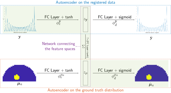
(a)

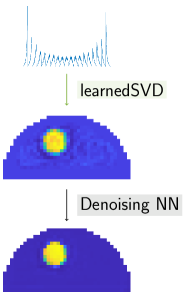
(b)

Figure 1: (a): Learned-SVD strategy for DOT reconstruction. The upper part of the scheme represents the dAE which receives as an input data ${\bm{y}}$ and outputs the reconstruction $\hat{{\bm{y}}}$. In doing this, denoise is also performed. Data are ordered in detector-source pairs as specified in the caption of Fig. 2. The bottom part represents the sAE which reconstructs the noise–free ground truth of the originating signal. The operator $\Sigma$ is learned in order to connect the two feature representations. The end-to-end workflow is enlightened in green and defines the mapping $\phi_{d}^{\mu}\circ\Sigma\circ\phi_{e}^{y}$; (b): test samples flow through the trained Learned-SVD NN and are further denoised to improve the results as in [20]. Abbreviations: FC = Fully Connected layer, tanh = hyperbolic tangent activation function, sigmoid = sigmoid activation function.

We follow here the Learned-SVD strategy introduced in [23], which aims at mimicking via a NN the SVD decomposition when its truncated or regularized version is employed. In order to understand the concept at the basis of this approach, it is useful to draw a parallel with the models introduced in the previous section. In this case, when the parameter-to–state operator $\mathcal{F}$ is linear, as it is for example using the Rytov strategy, one may write $\mathcal{F}={\bm{U}}{{\bm{S}}}{\bm{V}}^{\top}$, where ${{\bm{S}}}$ is a diagonal matrix containing the singular values and write the solution by the inversion formula $\mathcal{F}^{-1}={\bm{V}}{{\bm{S}}}^{-1}{\bm{U}}^{\top}$. This idea is extended here to more general nonlinear parameter-to-state operators, which are not formally known from a model but directly learnt by data. Namely, one learns a generalized SVD decomposition via a special class of NNs called autoencoder (AE) architectures. To do this, similarly to [23], we consider two AEs: the first, called data-AE (dAE), acts on data ${\bm{y}}$ and is defined by

$${\bm{z}}_{\bm{y}}=\phi_{e}^{y}({\bm{y}}),\qquad\hat{{\bm{y}}}=\phi_{d}^{y}({\bm{z}}_{\bm{y}}),$$ (18)

where ${\bm{z}}_{\bm{y}}$ is the encoded feature (latent representation) of the noisy data ${\bm{y}}$ and $\hat{{\bm{y}}}$ its decoded version. In the SVD framework, $\phi_{e}^{\bm{y}}$ and $\phi_{d}^{\bm{y}}$ can be seen as the correspective of ${\bm{U}}^{\top}$ and ${\bm{U}}$ for the linear case, respectively. This encoder–decoder has also by construction a denoising behaviour since the AE is trained in order to yield a noise–free reconstruction of the noisy input. The second AE, called signal–AE (sAE), acts on the generating signal and is defined by

$${\bm{z}}_{\mu}=\phi_{e}^{\mu}({{\bm{\mu}}_{a}}),\qquad\widehat{{\bm{\mu}}}_{a}=\phi_{d}^{\mu}({{\bm{\mu}}_{a}}),$$ (19)

where ${\bm{z}}_{\mu}$ is the encoded feature (latent representation) of the generating signal ${\bm{\mu}}_{a}$ and $\widehat{{\bm{\mu}}}_{a}$ its decoded version. Within the SVD framework, the decoder $\phi_{d}^{\mu}$ can be considered as the counterpart of ${\bm{V}}$. The two latent feature representations ${\bm{z}}_{\bm{y}}$ and ${\bm{z}}_{\mu}$ are related by a bridging operator $\Sigma$, such that ${\bm{z}}_{\mu}=\Sigma({\bm{z}}_{\bm{y}})$, which plays the scaling role of the singular values in ${\bm{S}}$ in the classical SVD approach.

The strategy consists thus in:

1. Encoding the data ${\bm{y}}$ in the latent space via the encoder $\phi_{e}^{y}$ (corresponds to perform the product ${\bm{U}}^{\top}{\bm{y}}$).

2. Connecting the latent variables ${\bm{z}}_{\bm{y}}$ and ${\bm{z}}_{\mu}$ via the operator $\Sigma$ (mimics the computation ${\bm{S}}^{-1}{\bm{U}}^{\top}{\bm{y}}$).

3. Decoding the latent variables ${\bm{z}}_{\mu}$ into the coefficient distribution via the decoder $\phi_{d}^{\mu}$ (corresponds to the final left multiplication by ${\bm{V}}$ in the SVD).

The parallelism of the proposed scheme with classical SVD is further represented by the scheme in (20).

(20)

Fig. 1 depicts the application of the Learned-SVD to the DOT context, which results in a fully data–driven method.

Remark 2

Tikhonov regularization and (truncated) SVD share a common role in regularization. Indeed, consider (15) with a linear operator and when $\mathcal{R}$ is chosen as $\frac{1}{2}\|\cdot\|_{2}^{2}$: the solution to this problem can be expressed using SVD as

$${\bm{\delta\mu}}_{a}^{*}=\sum_{i}f_{\alpha}(\sigma_{i})\left\langle{\bm{u}}_{i},{\bm{y}}\right\rangle\,{\bm{v}}_{i},$$

where ${\bm{v}}_{i}$ and ${\bm{u}}_{i}$ are the $i$–th right and left eigenvectors and $\sigma_{i}$ is the $i$–th singular value of ${\bm{J}}$, respectively, and where the function $f_{\alpha}(\sigma)=\frac{\sigma}{\sigma^{2}+\alpha}$ filters out the smaller singular values, according to the threshold $\alpha$ (regularization parameter). While in the classical approach this parameter is chosen a-priori and used in the specific function $f_{\alpha}(\sigma)$, the Learned-SVD approach learns the operator $\Sigma$ which plays the role of the filtering function $f$ and doses automatically the amount of required regularization. In doing so, it learns at the same time the regularization functional $\mathcal{R}$ and the parameter $\alpha$, which are both encompassed in $\Sigma$.

Remark 3

Notice that in the Learned-SVD approach, ${\bm{y}}$ directly represents the measurements $u|_{\bm{d}}$ and not the logarithmic amplitude fluctuation, since no linearization has been performed. As a consequence, the reconstruction yields the full absorption coefficient vector.

V Results

We assessed the performance of the proposed NN-based approach via quantitative indices and we compared it to the results obtained with variational regularization obtained via the Elastic-Net penalization or the Bregman approach. Experiments were carried out on a synthetic phantom both in noise–free and noisy conditions. All the numerical experiments were carried on a laptop PC with operating system Linux 22.04, endowed with an Intel(R) Core(TM) i5–8250U CPU (1.60GHz) and 16 GiB RAM memory. The NN architectures were implemented in MatLab®R2022a using the Deep Learning Toolbox^TM.

V-A Generation of synthetic data

We considered synthetic measures generated via the DE forward model discretized by an in–house finite element code using a fine mesh. The domain consists in a 2D semidisk with radius 5 cm, with 19 light sources positioned 1 mm inside the straight boundary and 20 detectors uniformly distributed on the semicircular portion of the boundary. The background coefficient was set to $\mu_{a,0}=0.01$ cm^-1 and we considered constant $(1-g)\mu_{s}=0.1$ cm^-1 (see Fig. 2) For reconstruction, we discretized the domain into square voxels with side 0.25 cm.

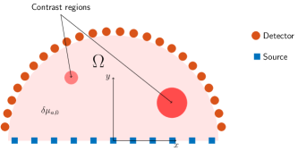
Figure 2: Geometry of the domain $\Omega$ considered in the numerical simulations. The detectors are uniformly disposed along the curved boundary with numeration progressing in counterclockwise sense starting from the rightmost detector; the sources are aligned along the bottom boundary and positioned 1mm inside $\Omega$, with numeration increasing from left to right. The absorption coefficient is $\mu_{a,0}$ except for the contrast regions which have increased absorption coefficient.

To train the network, we generated a set of 1500 samples, each including one or two circular contrast regions with random radius and position inside the domain. The contrast regions were chosen to have absorption coefficient equal to $3,4$ or $5$-fold the background coefficient. When there were two contrast regions, each region was allowed to have different absorption coefficient. The test dataset used to evaluate the performance of the network and to compare it with the variational approaches contained 150 samples built according to the same rules as above. In our experiments, we considered noise-free data as well as noisy measures, obtained by adding white Gaussian noise to the fluence values at the detectors with variance 1%, 3% or 5%, respectively.

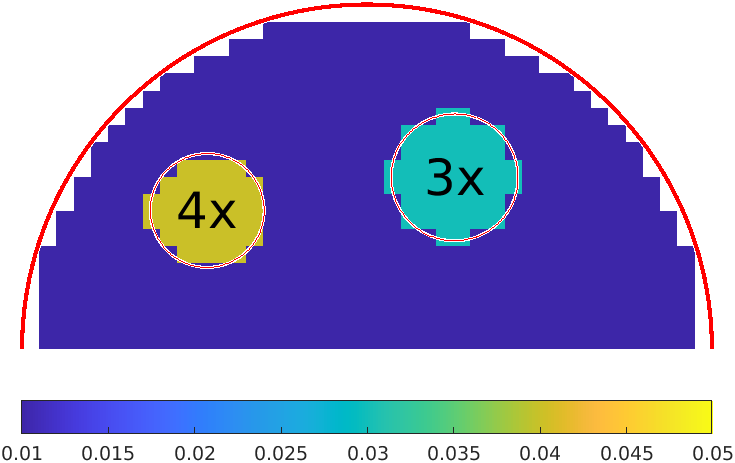
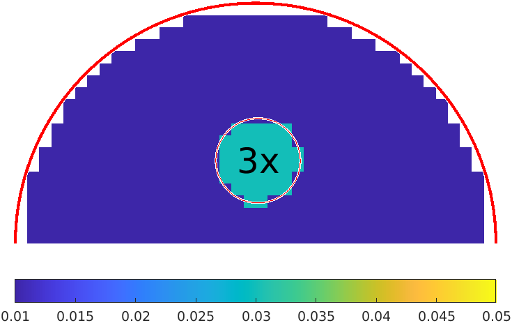
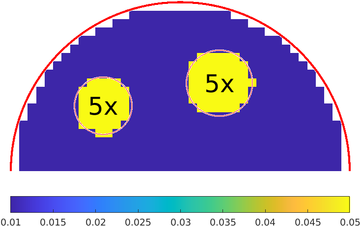
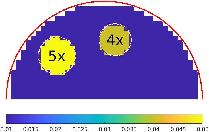
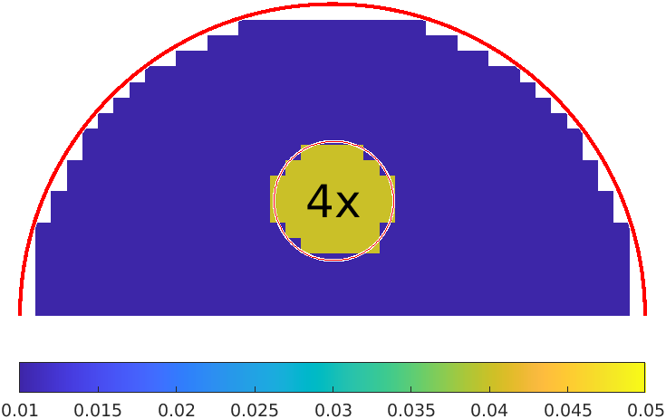
(a)

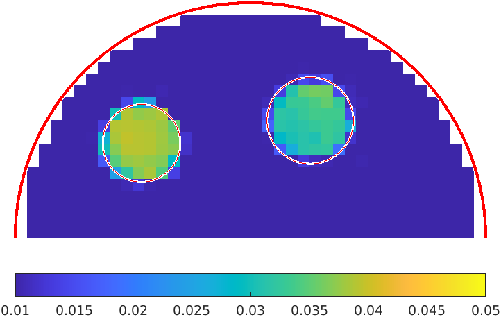
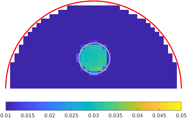
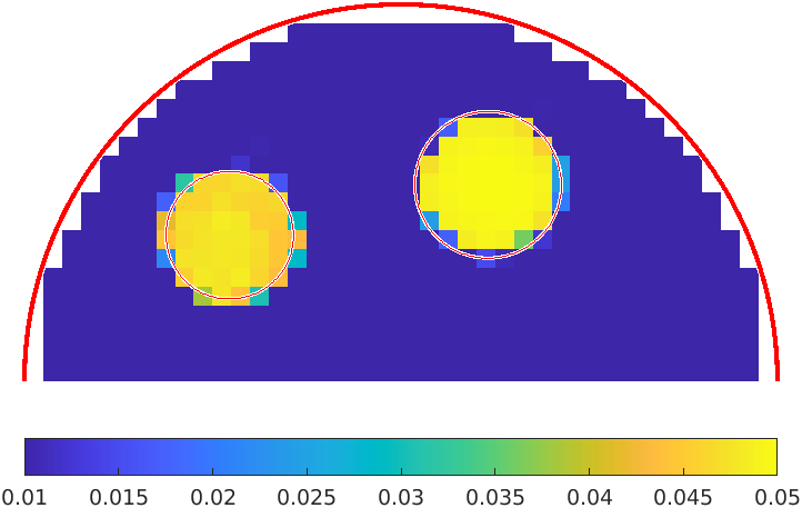
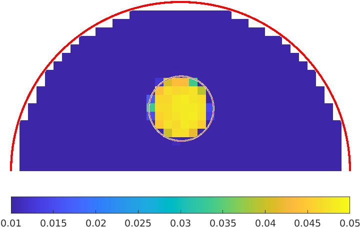
(b)

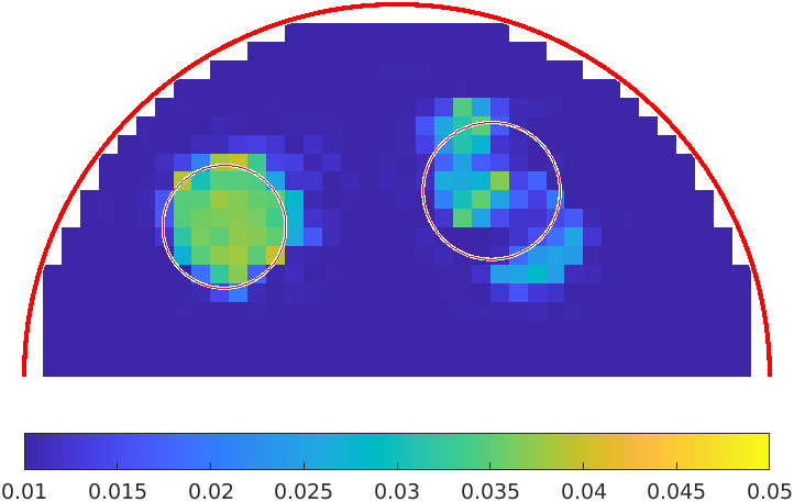
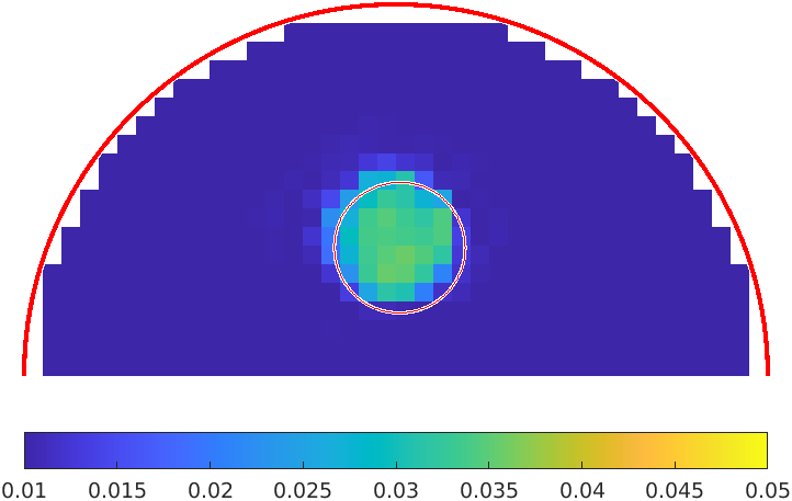
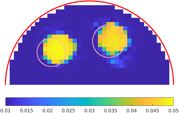
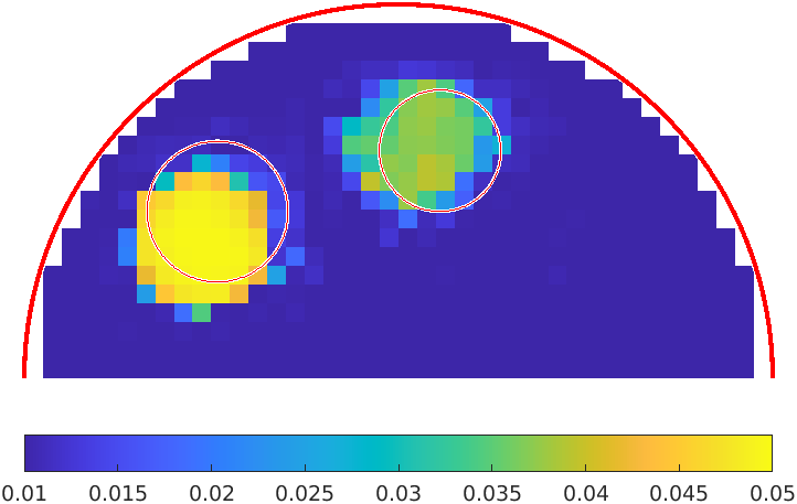
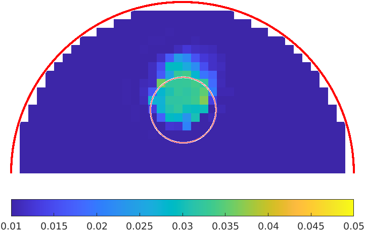
(c)

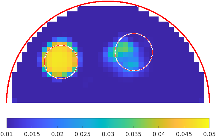
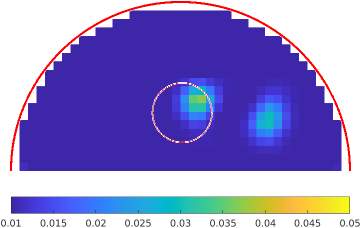
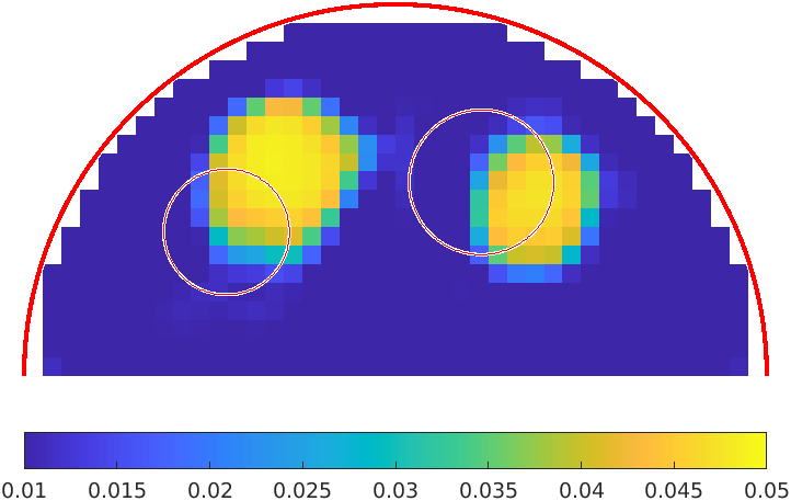
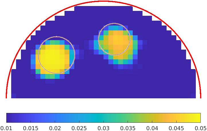
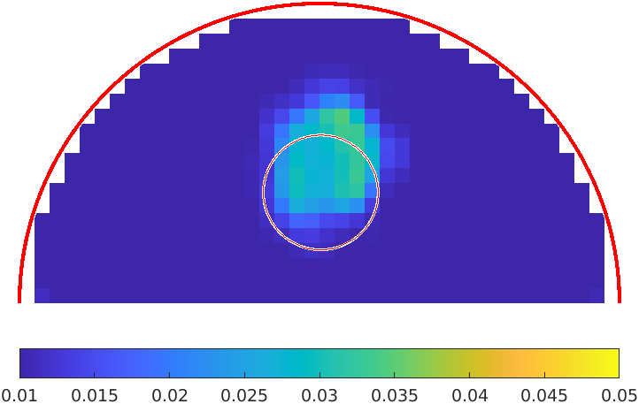
(d)

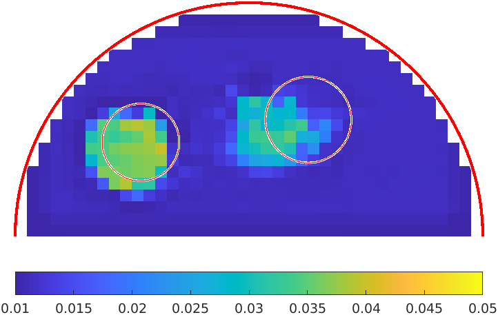
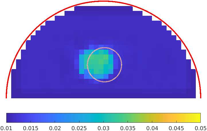
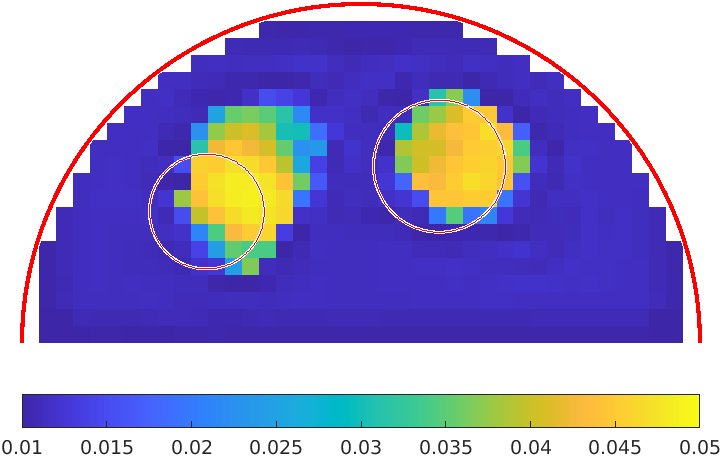
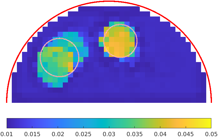
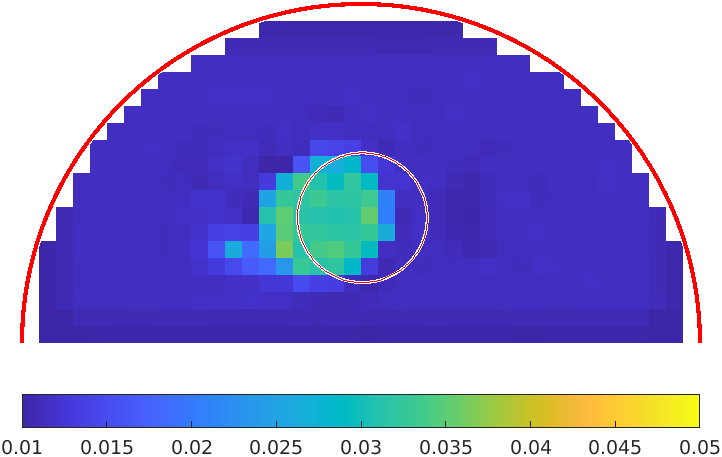
(e)

Figure 3: Reconstruction of the absorption coefficient distribution obtained with the Learned-SVD approach. (3a) Ground truth. The red circles denote the true contrast regions along with the corresponding absorption coefficient, expressed as a multiplier of the background value. (3b): noise-free case, (3c): 1% noise, (3d): 3% noise, (3e): 5% noise.

V-B Learned-SVD: implementation of the network

Both the encoders in the dAE and in sAE nets were chosen as fully connected layers coupled with a $\tanh$ activation function, while both the corresponding decoders were chosen as a fully connected layer plus a sigmoid function. We investigated several options for the architecture of the $\Sigma$ bridge operator. Experiments showed that the best architecture was formed by 7 layers, each one consisting in a fully connected layer plus a $\tanh$ activation function. The training of the NNs was performed via the Stochastic Gradient Descent method, with default settings. The training strategy was the following: the dAE and the sAE were trained separately, with learning rate of 0.1 and 0.01, respectively. For each AE network, the loss function was chosen as the Euclidean distance between the ground truth and the reconstructed data. The number of epochs was 2000 for each training procedure. The $\Sigma$ network was trained on the dataset formed by the hidden representations of the two AE networks, with a learning rate 0.1. The final trained Learned-SVD network (cf. Figure 1a, green shaded area) was created by connecting the layers of the encoder of dAE, of the network $\Sigma$ and of the decoder of sAE. The Learned-SVD net provided good results, but artifacts were still present: in order to remove them, we added a downstream NN with the role of a further denoiser. For this latter net we used the same architecture of [20]. An illustration of the end–to–end workflow is provided in Fig. 1b.

V-C Variational Approaches

To carry out a comparison of the results obtained with the Learned-SVD approach with classical variational methods we considered two approaches that we had used in our past research work in the Rytov setting:

Elastic Net regularization [11]

we look for

$$\operatorname*{argmin}_{{\bm{\delta\mu}}_{a}}\frac{1}{2}\|{\bm{J}}\,{\bm{\delta\mu}}_{a}-{\bm{y}}\|+\alpha\left(\vartheta\|{\bm{\delta\mu}}_{a}\|_{1}+(1-\vartheta)\|{\bm{\delta\mu}}_{a}\|_{2}^{2}\right),$$

$\vartheta\in[0,1]$. In this case, $\mathcal{R}$ is a convex combination of $\ell_{2}$ and $\ell_{1}$ norms, which aims at merging the best characteristics of both regularization functionals: the sparse–promoting and peak-enhancing property of the $\ell_{1}$ norm and the robustness of the Tikhonov regularization. The solution is computed using the MatLab implementation of glmnet [38], a highly efficient package that fits generalized linear and similar models via penalized maximum likelihood. Cross validation is used to obtain the optimal regularization parameter. In the numerical experiments $\vartheta$ is set to 0.5.

Bregman approach [15, 13]

it is an iterative strategy where at each step $\mathcal{R}$ is substituted with its Bregman Divergence computed at the previous iterate. If $\mathcal{R}$ satisfies suitable hypotheses (namely, being a convex, proper, lower semicontinuous function) and denoting by $\partial\mathcal{R}(\bm{\xi})$ the subdifferential of $\mathcal{R}$ computed at ${\bm{\xi}}$ (see [39] for technical details), then the Bregman divergence of $\mathcal{R}$ is

$$D_{\mathcal{R}}^{{\bm{p}}}({\bm{\xi}},{\bm{\eta}})=\mathcal{R}({\bm{\xi}})-\mathcal{R}({\bm{\eta}})-\langle{\bm{p}},{\bm{\xi}}-{\bm{\eta}}\rangle,\quad{\bm{p}}\in\partial\mathcal{R}({\bm{\xi}}).$$

The functional to minimize at the $k+1$–th step is thus

$$\frac{1}{2}\|{\bm{J}}\,{\bm{\delta\mu}}_{a}-{\bm{y}}\|_{2}^{2}+\alpha D_{\mathcal{R}}^{{\bm{p}}^{k}}({\bm{\delta\mu}}_{a},{\bm{\delta\mu}}_{a}^{k})$$

where ${\bm{p}}^{k}\in\partial\mathcal{R}({\bm{\delta\mu}}_{a}^{k})$. Discarding the constant terms and considering the optimality conditions, the whole procedure consists in a two–step strategy

$${\bm{\delta\mu}}_{a}^{k+1}=\operatorname*{argmin}_{{\bm{\delta\mu}}_{a}}\frac{1}{2}\|{\bm{J}}\,{\bm{\delta\mu}}_{a}-{\bm{y}}\|_{2}^{2}+ \alpha\mathcal{R}({\bm{\delta\mu}}_{a})+$$

$$-\alpha\langle{\bm{p}}^{k},{\bm{\delta\mu}}_{a}\rangle$$ (21)

$${\bm{p}}^{k+1}={\bm{p}}^{k}-\frac{1}{\alpha}{\bm{J}}^{\top}\left({\bm{J}}\,{\bm{\delta\mu}}_{a}-{\bm{y}}\right)$$ (22)

The Bregman procedure was coupled with the choice of $\ell_{1}$ regularization. The inner sub problem (V-C) is dealt with the Forward–Backward algorithm [40], which consists in solving the general problem

$$\min_{\bm{\eta}}f_{0}({\bm{\eta}})+f_{1}({\bm{\eta}})$$

via an iterative scheme

$${\bm{x}}^{k+1}\leftarrow\operatorname*{argmin}_{{\bm{x}}}f_{0}({\bm{x}}^{k})+\frac{1}{2\gamma}\|{\bm{x}}-\left({\bm{x}}^{k}-\gamma\nabla f_{1}({\bm{x}})\right)\|_{2}^{2}$$

In view of (V-C), $f_{1}(\cdot)=\frac{1}{2}\|{\bm{J}}\cdot-y\|_{2}^{2}-\alpha\left\langle\cdot,{\bm{p}}\right\rangle$ and $f_{0}(\cdot)=\|\cdot\|_{1}$. The complete procedure is depicted in Algorithm 1, where $\operatorname*{soft}({\bm{\eta}})$ stands for the component–wise soft thresholding $\operatorname*{soft}_{\beta}(\eta)=\operatorname*{sign}(\eta)\max\{0,|{\eta}|-\beta\}$. The convergence of this approach has been proved in several previous works [41, 42, 15, 43].

Algorithm 1 Bregman Procedure with $\ell_{1}$ regularization

  Set ${\bm{\delta\mu}}_{a}^{0}$ such that ${\bm{p}}^{0}=\bm{0},{\bm{p}}^{0}\in\partial\mathcal{R}({\bm{\delta\mu}}_{a}^{0})$, set $\alpha>0,\,\gamma>0$.

  for $k=0,1,\dots$ do

     ${\bm{x}}^{\star}\leftarrow{\bm{\delta\mu}}_{a}^{k}$

     for $l=0,1,\dots$ do

        ${\bm{z}}^{l}\leftarrow({\bm{I}_{d}}-\gamma{\bm{J}}^{\top}{\bm{J}}){\bm{x}}^{\star}+\gamma({\bm{J}}^{\top}{\bm{y}}+{\bm{p}}^{k})$

        ${\bm{x}}^{\star}\leftarrow\operatorname*{soft}_{\gamma\alpha}({\bm{z}}^{l})$

     end for

     ${\bm{\delta\mu}}_{a}^{k}\leftarrow{\bm{x}}^{\star}$

     ${\bm{p}}^{k+1}\leftarrow{\bm{p}}^{k}-\displaystyle\frac{1}{\alpha}{\bm{J}}^{\top}\left({\bm{J}}\,{\bm{\delta\mu}}_{a}^{k}-{\bm{y}}\right)$

  end for

The algorithm is stopped when the number or outer iterations reaches 100, whilst the inner solver runs for 50 iterations. The regularization parameter $\alpha$ was set to $1.5\,\|{\bm{J}}^{\top}\,{\bm{y}}\|_{\infty}$ and $\gamma=0.99/\|{\bm{J}}^{\top}\,{\bm{J}}\|$.

Remark 4

With an abuse of notation, within the variational framework ${\bm{y}}$ denotes the algorithm fluctuation $\log(u/u_{0})$, recalling that ${u_{0}}$ are the measurements corresponding to unperturbed background conditions, and $u$ refers to condition (e.g. compression of the tissue) in which the lightpath is perturbed by the presence of pathological regions.

V-D Numerical results: qualitative and quantitative evaluation

Figure 3 presents the results obtained for five different samples in the test set with varying levels of noise. The red circles depict the exact position and radius of the contrast region (ground–truth). In the noise-free case, the perturbed regions is almost perfectly recovered, both in location, shape and intensity. The other rows refer to the reconstruction obtained when Gaussian noise affects the measure. As one expects, the increasing noise level worsens the quality of the reconstruction but the gross location and shape of the perturbed region are correctly captured. The results obtained via the Learned-SVD approach are compared with the ones obtained by the two considered variational frameworks in Fig. 4 (Elastic-Net) and in Fig. 5 (Bregman), respectively. These figures show the results for test cases of columns 1, 3 and 5 in Fig. 3a. Observe as already in the noise–free case (first row) we do not obtain truly reliable results due to the low resolution of the voxelization. Moreover, as the noise level increases the reconstruction quality significantly deteriorates, so that noise level 5% was not reported due to complete lack of significance.

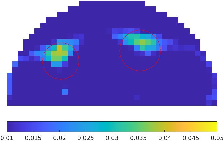
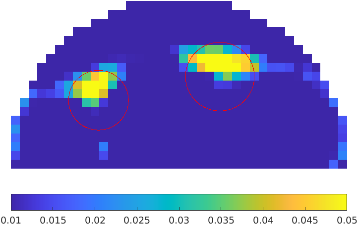
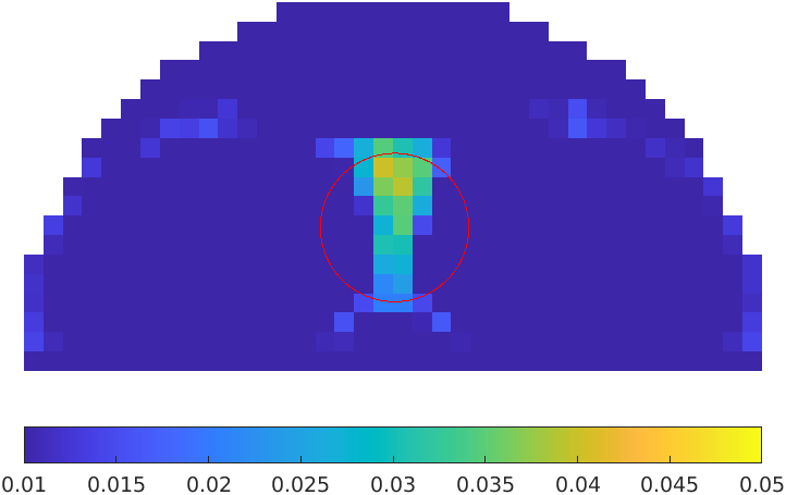
(a)

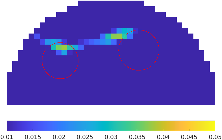
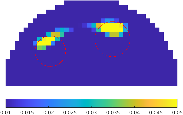
(b)

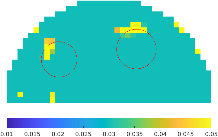
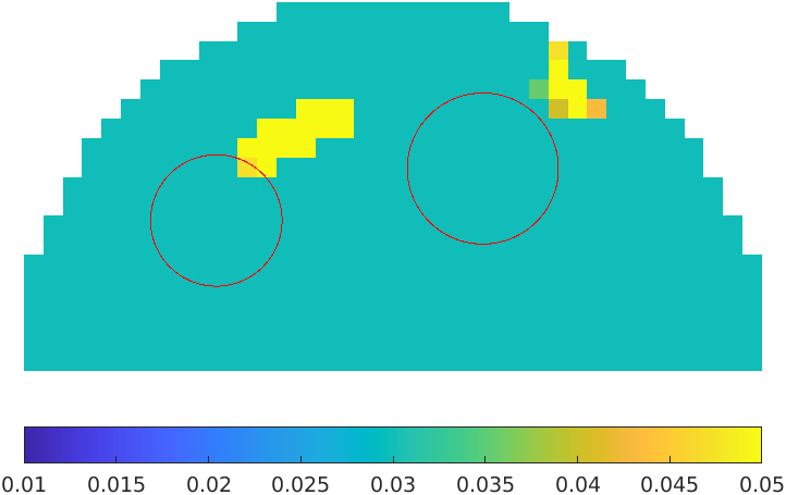
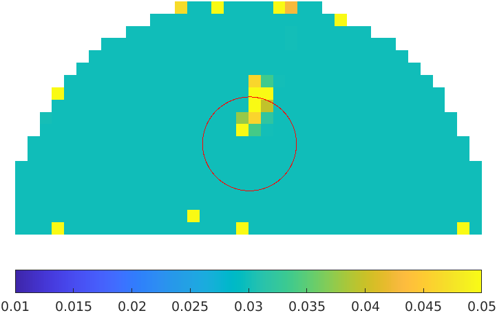
(c)

Figure 4: Reconstruction via the Elastic Net approach. 4a): noise-free case, 4b): 1% noise, 4c): 3% noise. The reconstruction are not reliable even in the noise free case due to the low resolution employed in these test.

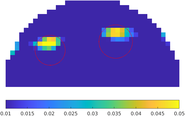
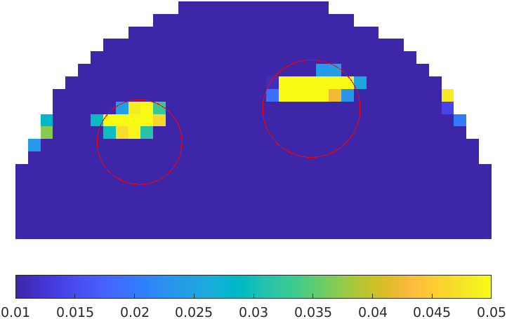
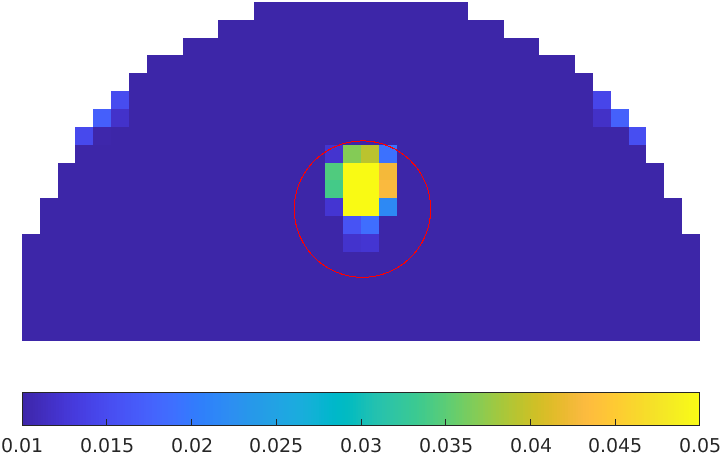
(a)

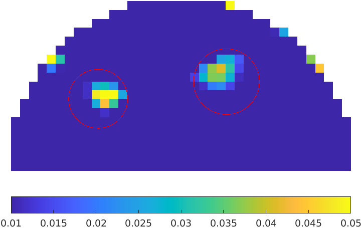
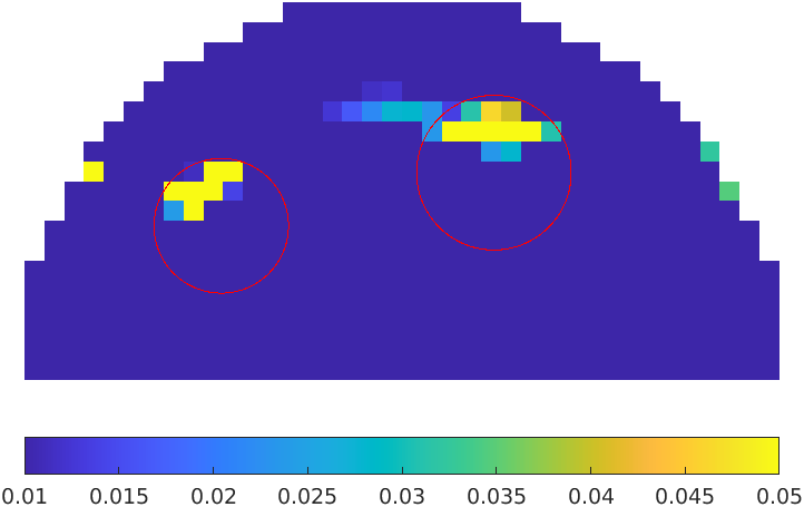
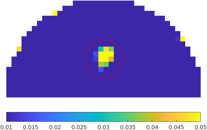
(b)

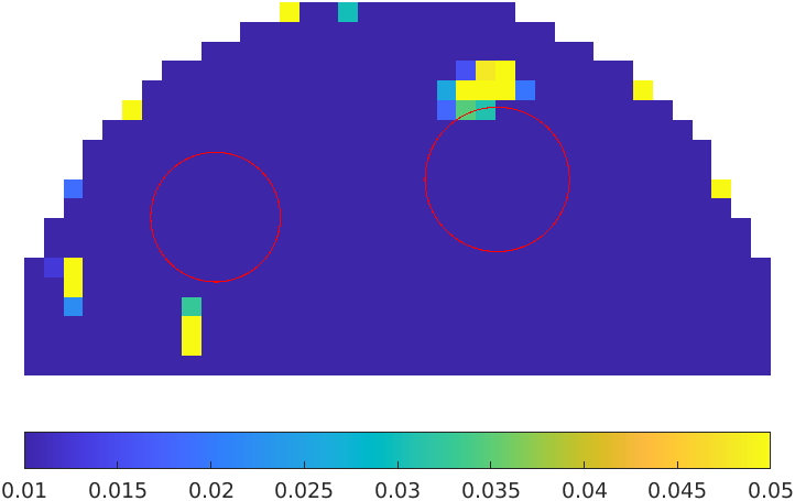
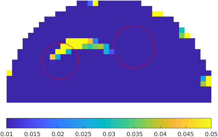
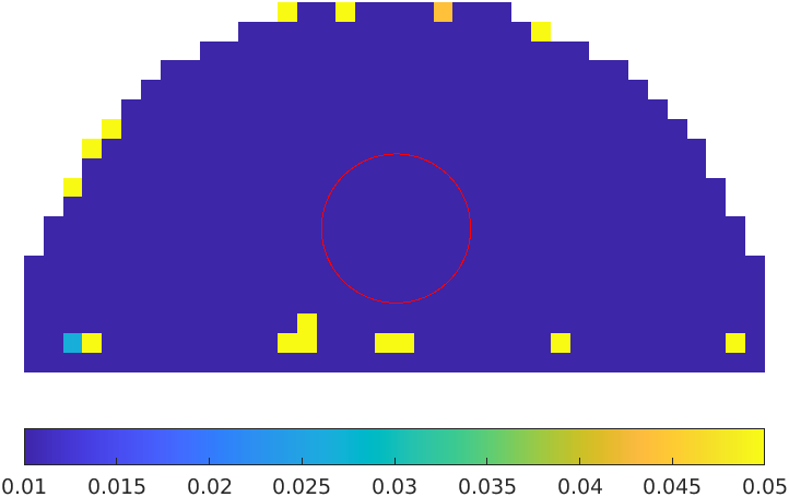
(c)

Figure 5: Reconstruction via the Bregman approach. 5a): noise-free case, 5b): 1% noise, 5c): 3% noise.

To quantitatively assess the performance of the proposed approach, we use two metrics. The first one is the average value of the absorption coefficient inside the reconstructed contrast regions (ACR), which aims to assess the accuracy of the reconstructed amplitude of the contrast. To evaluate the ACR we first need to determine the extend of the computed contrast regions by recognizing the connected components in the reconstructed image and assigning each of them to the contrast region which minimizes the distance between with the centroid of the pixel cloud. The second metric we use is the True Positive Ratio (TPR), which assesses the spatial accuracy of the positioning of the reconstructed contrast regions by checking how many pixels in the reconstruction actually belong to the true contrast region. The results of the two metrics are summarized in Table I, which presents their averages on the 150 samples of the test set for the Learned-SVD approach and, for comparison, of the considered variational approaches. Notice that the ACR results have been binned according to the intensity of the contrast region.

TABLE I: ACR (binned according to the intensity of the contrast region) and TPR metrics for different noise levels. Values are averaged over 150 test samples.

Noise Level	${3\mu_{a,0}}$ (GT: 3e-2)	${4\mu_{a,0}}$ (GT: 4e-2)	${5\mu_{a,0}}$ (GT: 5e-02)	TPR
	Learned-SVD
0%	3.05e-02 $\pm$ 2.00e-03	4.08e-02 $\pm$ 3.72e-03	4.74e-02 $\pm$ 2.19e-03	0.94
1%	3.07e-02 $\pm$ 2.77e-03	3.76e-02 $\pm$ 5.54e-03	4.38e-02 $\pm$ 4.01e-03	0.76
3%	3.06e-02 $\pm$ 5.56e-03	3.61e-02 $\pm$ 6.10e-03	4.11e-02 $\pm$ 4.65e-03	0.52
5%	3.00e-02 $\pm$ 3.82e-03	3.15e-02 $\pm$ 4.44e-03	3.39e-02 $\pm$ 6.04e-03	0.46
	Elastic Net
0%	2.73e-02 $\pm$ 4.74e-03	3.45e-02 $\pm$ 4.96e-03	3.90e-02 $\pm$ 8.69e-03	0.45
1%	2.91e-02 $\pm$ 9.36e-03	4.30e-02 $\pm$ 8.70e-03	5.01e-02 $\pm$ 9.80e-03	0.17
3%	9.55e-02 $\pm$ 1.92e-02	1.25e-01 $\pm$ 2.83e-02	1.23e-01 $\pm$ 3.36e-02	0.05
	Bregman
0%	4.02e-02 $\pm$ 8.95e-03	5.93e-02 $\pm$ 1.61e-02	8.54e-02 $\pm$ 2.98e-02	0.26
1%	4.77e-02 $\pm$ 1.81e-02	5.85e-02 $\pm$ 1.84e-02	8.34e-02 $\pm$ 2.85e-02	0.17
3%	1.28e-01 $\pm$ 5.50e-02	1.45e-01 $\pm$ 9.06e-02	1.36e-01 $\pm$ 6.80e-02	0.03

For all the considered approaches, increasing levels of noise significantly worsen the TPR, as well as the ACR. However, the quality loss exhibited by the Learned-SVD approach is significantly less pronounced, especially for the ACR metric. As a matter of fact, the reconstructed regions with the NN-based method still show a notable contrast with respect to the background value, and 46% of the extension of the perturbed regions is correctly recovered on average even for the highest noise level (vs 5% and 3% for the variational approaches, respectively). One should notice that in the Elastic Net approach the reconstructed intensities constantly approximate the nominal one by defect for low noise level: this is not fully surprising, since regularization comes at the cost of a certain degree of smearing/blurring of the solution. On the other hand, Bregman technique increases the contrast, as already observed in previous works. In presence of high level of noise, the results are completely unreliable. Classic variational methods suffer from this problem to a higher degree especially for a rather coarse voxelization as the one we considered here (results, not reported here, for finer voxelizations, do confirm in any case this general trend).

VI Conclusions

DOT reconstruction is a severely ill-conditioned problem which demands a robust regularization to obtain reasonable results. Commonly used strategies are based on physics-driven models accompanied by priors which enforce constraints on the variance of the solution or in its sparsity. These strategies often fail or are computationally very intesive. In this work we have investigated a NN-based regularization technique, inspired by the Learned-SVD method originally proposed in [23] for general inverse problem. This approach is a fully data–driven strategy which adopts two AEs bridged by an operator which mimics the effect of a (truncated) singular value matrix. The Learned-SVD produces significantly improved results with respect to classic variational approaches based on $L^{p},p\geq 1,$ penalization. According to the measured metrics, the present NN-based strategy yields an average 94% TPR for noise–free data and for higher levels of noise the deterioration of the results is signifiantly less severe than for variational methods, even for a coarse voxelization of the domain. The training of the net performed in this work was based on a purely synthetic dataset: results obtained by other authors (see for example [44]) show that such an approach can convey good performances even when networks trained in such a way are used in realistic conditions. Transfer learning techniques could also be employed to improve the reliability of the net on realistic datasets, even in presence of a limited number of available samples. Future work will be focused on the idea of exporting and adapting techniques from low-dose X-ray CT (another ill-conditioned problem) to the present context, with a specific attention for the hybrid integration with information coming from the rich physical models describing light propagation in tissues.

VII Acknowledgments.

AB and PC received support by the SEED-PRECISION project, funded by University of Milan. PC also acknowledges support from Italian Ministry of Research PRIN project NA_FROM-PDEs.

References

- [1] Y. Hoshi and Y. Yamada, “Overview of diffuse optical tomography and its clinical applications,” Journal of biomedical optics, vol. 21, no. 9, p. 091312, 2016.
- [2] Y. Yamada and S. Okawa, “Diffuse optical tomography: Present status and its future,” Optical Review, vol. 21, no. 3, pp. 185–205, 2014.
- [3] H. Jiang, Diffuse Optical Tomography: Principles and Applications. CRC Press, 2018.
- [4] S. R. Arridge, “Optical tomography in medical imaging,” Inverse problems, vol. 15, no. 2, p. R41, 1999.
- [5] D. Boas, D. Brooks, E. Miller, C. DiMarzio, M. Kilmer, R. Gaudette, and Q. Zhang, “Imaging the body with diffuse optical tomography,” IEEE Signal Processing Magazine, vol. 18, no. 6, pp. 57–75, 2001.
- [6] S. R. Arridge and J. C. Schotland, “Optical tomography: forward and inverse problems,” Inverse problems, vol. 25, no. 12, p. 123010, 2009.
- [7] O. Lee, J. M. Kim, Y. Bresler, and J. C. Ye, “Compressive diffuse optical tomography: Noniterative exact reconstruction using joint sparsity,” IEEE Transactions on Medical Imaging, vol. 30, no. 5, pp. 1129–1142, 2011.
- [8] H. Egger and M. Schlottbom, “Analysis and regularization of problems in diffuse optical tomography,” SIAM Journal on Mathematical Analysis, vol. 42, no. 5, pp. 1934–1948, 2010.
- [9] H. O. Kazanci and S. L. Jacques, “Diffuse light tomography to detect blood vessels using Tikhonov regularization,” in Saratov Fall Meeting 2015: Third International Symposium on Optics and Biophotonics and Seventh Finnish-Russian Photonics and Laser Symposium (PALS), E. A. Genina, V. V. Tuchin, V. L. Derbov, D. E. Postnov, I. V. Meglinski, K. V. Larin, and A. B. Pravdin, Eds., vol. 9917, International Society for Optics and Photonics. SPIE, 2016, pp. 202 – 210. [Online]. Available: https://doi.org/10.1117/12.2230074
- [10] S. Okawa, Y. Hoshi, and Y. Yamada, “Improvement of image quality of time-domain diffuse optical tomography with lp sparsity regularization,” Biomed. Opt. Express, vol. 2, no. 12, pp. 3334–3348, Dec 2011. [Online]. Available: http://opg.optica.org/boe/abstract.cfm?URI=boe-2-12-3334
- [11] P. Causin, G. Naldi, and R. Weishaeupl, “Elastic net regularization in diffuse optical tomography applications,” in 2019 IEEE 16th International Symposium on Biomedical Imaging (ISBI 2019), 2019, pp. 1627–1630.
- [12] P. Causin, M. G. Lupieri, G. Naldi, and R.-M. Weishaeupl, “Mathematical and numerical challenges in optical screening of female breast,” International Journal for Numerical Methods in Biomedical Engineering, vol. 36, no. 2, p. e3286, 2020.
- [13] A. Benfenati, P. Causin, M. Lupieri, and G. Naldi, “Regularization techniques for inverse problem in DOT applications,” Journal of Physics: Conference Series, vol. 1476, p. 012007, mar 2020.
- [14] X. Zhang, M. Burger, and S. Osher, “A unified primal-dual algorithm framework based on Bregman iteration,” Journal of Scientific Computing, vol. 46, no. 1, pp. 20–46, 2011.
- [15] A. Benfenati and V. Ruggiero, “Inexact Bregman iteration with an application to Poisson data reconstruction,” Inverse Problems, vol. 29, no. 6, 2013.
- [16] A. Benfenati, A. La Camera, and M. Carbillet, “Deconvolution of post-adaptive optics images of faint circumstellar environments by means of the inexact Bregman procedure,” Astronomy and Astrophysics, vol. 586, 2016.
- [17] A. Benfenati and V. Ruggiero, “Inexact Bregman iteration for deconvolution of superimposed extended and point sources,” Communications in Nonlinear Science and Numerical Simulation, vol. 20, no. 3, pp. 882–896, 2015.
- [18] M. Schweiger and S. R. Arridge, “The TOAST++ software suite for forward and inverse modeling in optical tomography,” J Biomed Opt, vol. 19, no. 4, p. 040801, 2014.
- [19] Z. Wu, Y. Sun, A. Matlock, J. Liu, L. Tian, and U. S. Kamilov, “SIMBA: Scalable inversion in optical tomography using deep denoising priors,” IEEE Journal of Selected Topics in Signal Processing, vol. 14, no. 6, pp. 1163–1175, 2020.
- [20] J. Yoo, S. Sabir, D. Heo, K. Kim, A. Wahab, Y. Choi, S.-I. Lee, E. Chae, H. Kim, Y. Bae, Y.-W. Choi, S. Cho, and J. Ye, “Deep learning diffuse optical tomography,” IEEE Transactions on Medical Imaging, vol. 39, no. 4, pp. 877–887, 2020.
- [21] M. Mozumder, A. Hauptmann, I. Nissilä, S. R. Arridge, and T. Tarvainen, “A model-based iterative learning approach for diffuse optical tomography,” arXiv preprint arXiv:2104.09579, 2021.
- [22] L. Zhang and G. Zhang, “Brief review on learning-based methods for optical tomography,” Journal of Innovative Optical Health Sciences, vol. 12, no. 06, p. 1930011, 2019.
- [23] Y. E. Boink and C. Brune, “Learned SVD: solving inverse problems via hybrid autoencoding,” CoRR, vol. abs/1912.10840, 2019.
- [24] S. Lunz, O. Öktem, and C.-B. Schönlieb, “Adversarial regularizers in inverse problems,” vol. 2018-December, 2018, p. 8507 – 8516.
- [25] E. Kobler, A. Effland, K. Kunisch, and T. Pock, “Total deep variation for linear inverse problems,” in Proceedings of the IEEE/CVF Conference on Computer Vision and Pattern Recognition (CVPR), June 2020.
- [26] ——, “Total deep variation: A stable regularizer for inverse problems,” CoRR, vol. abs/2006.08789, 2020.
- [27] H. Li, J. Schwab, S. Antholzer, and M. Haltmeier, “NETT: solving inverse problems with deep neural networks,” Inverse Problems, vol. 36, no. 6, p. 065005, jun 2020.
- [28] H. Vavadi and Q. Zhu, “Automated data selection method to improve robustness of diffuse optical tomography for breast cancer imaging,” Biomedical optics express, vol. 7, no. 10, pp. 4007–4020, 2016.
- [29] T. Durduran, R. Choe, W. B. Baker, and A. G. Yodh, “Diffuse optics for tissue monitoring and tomography.” Reports on progress in physics. Physical Society, vol. 73 7, 2010.
- [30] M. Mansuripur, Classical optics and its applications. Cambridge University Press, 2002.
- [31] A. Ishimaru, Wave propagation and scattering in random media. Academic Press New York, 1978, vol. 2.
- [32] P. Causin and R.-M. Weishaeupl, “Inverse problems in diffuse optical tomography applications,” in Mathematical Modelling in Real Life Problems. Springer, 2020, pp. 1–16.
- [33] G. Di Sciacca, L. Di Sieno, A. Farina, P. Lanka, E. Venturini, P. Panizza, A. Dalla Mora, A. Pifferi, P. Taroni, and S. Arridge, “Enhanced diffuse optical tomographic reconstruction using concurrent ultrasound information,” Philosophical Transactions of the Royal Society A, vol. 379, no. 2204, p. 20200195, 2021.
- [34] C. Panagiotou, S. Somayajula, A. P. Gibson, M. Schweiger, R. M. Leahy, and S. R. Arridge, “Information theoretic regularization in diffuse optical tomography,” J. Opt. Soc. Am. A, vol. 26, no. 5, pp. 1277–1290, May 2009.
- [35] N. Cao, A. Nehorai, and M. Jacob, “Image reconstruction for diffuse optical tomography using sparsity regularization and expectation-maximization algorithm,” Opt. Express, vol. 15, no. 21, pp. 13 695–13 708, Oct 2007. [Online]. Available: http://opg.optica.org/oe/abstract.cfm?URI=oe-15-21-13695
- [36] N. Meinshausen and P. Bühlmann, “High-dimensional graphs and variable selection with the lasso,” The annals of statistics, vol. 34, no. 3, pp. 1436–1462, 2006.
- [37] A. Yodh and B. Chance, “Spectroscopy and imaging wih diffusing light,” Physics Today, vol. 48, no. 3, pp. 34–40, 1995.
- [38] J. Friedman, T. Hastie, and R. Tibshirani, “Regularization paths for generalized linear models via coordinate descent,” Journal of Statistical Software, vol. 33, no. 1, pp. 1–22, 2010. [Online]. Available: https://www.jstatsoft.org/v33/i01/
- [39] R. Rockafellar, Convex Analysis: (PMS-28), ser. Princeton Landmarks in Mathematics and Physics. Princeton University Press, 2015.
- [40] P. L. Combettes and J.-C. Pesquet, “Fixed point strategies in data science,” IEEE Transactions on Signal Processing, vol. 69, pp. 3878–3905, 2021.
- [41] W. Yin, S. Osher, D. Goldfarb, and J. Darbon, “Bregman iterative algorithms for -minimization with applications to compressed sensing,” SIAM Journal on Imaging Sciences, vol. 1, no. 1, pp. 143–168, 2008.
- [42] X. Zhang, M. Burger, X. Bresson, and S. Osher, “Bregmanized nonlocal regularization for deconvolution and sparse reconstruction,” SIAM Journal on Imaging Sciences, vol. 3, no. 3, pp. 253–276, 2010.
- [43] P. L. Combettes and V. R. Wajs, “Signal recovery by proximal forward-backward splitting,” Multiscale Modeling & Simulation, vol. 4, no. 4, pp. 1168–1200, 2005.
- [44] S. Sabir, S. Cho, Y. Kim, R. Pua, D. Heo, K. H. Kim, Y. Choi, and S. Cho, “Convolutional neural network-based approach to estimate bulk optical properties in diffuse optical tomography,” Applied Optics, vol. 59, no. 5, pp. 1461–1470, 2020.