An Exact Method for Fortification Games

Abstract

A fortification game (FG) is a three-level, two-player Stackelberg game, also known as defender-attacker-defender game, in which at the uppermost level, the defender selects some assets to be protected from potential malicious attacks. At the middle level, the attacker solves an interdiction game by depreciating unprotected assets, i.e., reducing the values of such assets for the defender, while at the innermost level the defender solves a recourse problem over the surviving or partially damaged assets. Fortification games have applications in various important areas, such as military operations, design of survivable networks, protection of facilities or power grid protection. In this work, we present an exact solution algorithm for FGs, in which the recourse problems correspond to (possibly NP-hard) combinatorial optimization problems. The algorithm is based on a new generic mixed-integer linear programming reformulation in the natural space of fortification variables. Our new model makes use of fortification cuts that measure the contribution of a given fortification strategy to the objective function value. These cuts are generated on-the-fly by solving separation problems, which correspond to (modified) middle-level interdiction games. We design a branch-and-cut-based solution algorithm based on fortification cuts, their strengthened versions and other speed-up techniques. We present a computational study using the knapsack fortification game and the shortest path fortification game. For the latter one, we include a comparison with a state-of-the-art solution method from the literature. Our algorithm outperforms this method and allows us to solve previously unsolved instances with up to 330 386 nodes and 1 202 458 arcs to optimality.

Keywords: Three-Level Optimization, Branch-and-Cut, Fortification Games, Shortest Path Fortification, Maximum Knapsack Fortification

1 Introduction

Fortification games (FGs), also known as defender-attacker-defender (DAD) problems, have applications in various important areas, such as military operations, the design of survivable networks, protection of facilities, or power grid protection (Lozano and Smith,, 2017; Smith and Song,, 2020). A FG is a three-level, two-player Stackelberg game: At the third (innermost) level the defender wants to solve some optimization problem (denoted as recourse problem) which depends on some resources (assets). At the second level, the attacker can select a subset of the assets to attack. Depending on the problem setting, this attack can either destroy the assets, or depreciate their usefulness for the defender. The goal of the attacker is to make the result of the optimization problem of the defender as worse as possible. Such a two-level attacker-defender problem described so far is known as interdiction game (IG) in which case the actions of the attacker are called interdictions. In FGs, the defender can prevent interdictions at the first (outermost) level by fortifying some of its assets against potential attacks. Assets that are fortified cannot be interdicted by the attacker.

We focus on a particular family of fortification games which is defined as follows. Let $N$ be the set of assets, $f_{i}\geq 0$ be the cost for fortification of each asset $i\in N$, and $B_{F}$ be the fortification budget. Similarly, let $g_{i}\geq 0$ be the interdiction cost for each asset $i\in N$, and $B_{I}$ be the interdiction budget. Finally, let $d_{i}\geq 0$ denote the depreciation of an asset $i\in N$ due to interdiction. In the following, we will denote by $w$, $x$ and $y$ the incidence vector of a fortification, an interdiction, and a recourse strategy, respectively. Accordingly, we denote by $W=\{w\in\{0,1\}^{n}:\sum_{i\in N}f_{i}w_{i}\leq B_{F}\}$ the set of feasible fortifications and by $X=\{x\in\{0,1\}^{n}:\sum_{i\in N}g_{i}x_{i}\leq B_{I}\}$ the set of possible interdictions if there would be no fortifications, where $n=|N|$. In addition, we let $X(w)=X\cap\{x\in\mathbb{R}^{n}:x\leq 1-w\}$ be the set of feasible interdictions for a given fortification strategy $w$, and we denote by $Y\subseteq\{0,1\}^{n}$ the feasible region of the recourse problem, which is assumed to be non-empty. Using these definitions, the FGs studied in this work can be defined as

$$z^{*}=\,\min_{w\in W}\,\max_{x\in X(w)}\, \min_{y\in Y}\,\left\{c^{T}y+\sum_{i\in N}d_{i}x_{i}y_{i}\right\}.$$ (0-1 FG)

Remark 1.

Notice that according to our definition of (0-1 FG), interdiction decisions do not affect the feasible region $Y$ of the recourse problem, and each such decision is associated with a cost increase/penalty $d_{i}\geq 0$. However, without loss of generality, this definition also allows to model problems in which the attacker prohibits the use of the interdicted assets, i.e., where $Y(x)=Y\cap\{y\in\mathbb{R}^{n}:y\leq 1-x\}$. In this case, the resulting problem

$$z^{*}=\,\min_{w\in W}\,\max_{x\in X(w)}\, \min_{y\in Y(x)}\,c^{T}y$$

can be reformulated as

$$z^{*}=\,\min_{w\in W}\,\max_{x\in X(w)}\, \min_{y\in Y}\,\left\{c^{T}y+\sum_{i\in N}\mathcal{M}_{i}x_{i}y_{i}\right\}$$

for sufficiently large $\mathcal{M}_{i}$ (see, e.g., Fischetti et al., (2019)), i.e., in problem (0-1 FG) we set $d_{i}:=\mathcal{M}_{i}$.

Finally, we notice that more general types of fortification games have been introduced in the literature. For example, Alderson et al., (2011) considered the case in which the feasible region of the innermost problem depends on $w$ as well (i.e., we have $Y(w,x)$ instead of $Y(x)$), whereas Brown et al., (2006) addressed situations in which the third level variables are not necessarily binary and there might exist some available capacity which is invulnerable to the attack (e.g., $y\leq u_{0}+u(1-x)$). These more general settings are out of scope of this paper, and we focus on a particular version defined by the problem (0-1 FG).

1.1 Contribution and Outline

In this work, we present an exact solution algorithm for (0-1 FG). The algorithm is based on a new generic mixed-integer programming (MIP) formulation for (0-1 FG) which makes use of valid inequalities, denoted as fortification cuts. These cuts are used to measure the objective function value for given fortification strategies, and are generated on-the-fly by solving separation problems, which correspond to (modified) IGs.

The detailed contribution and outline is summarized as follows.

• We present a general solution framework for the problem (0-1 FG) whose recourse can be an arbitrary (possibly NP-hard) combinatorial optimization problem with linear objective function and discrete variables. Thus, we extend theory and methodology of the existing exact algorithms for fortification games, the majority of which requires the recourse problems to be convex.

• We introduce a single-level MIP reformulation for (0-1 FG) using fortification cuts, present alternative methods for strengthening these cuts, and discuss their efficient separation.

• We propose further algorithmic enhancements, that allow to speed-up the separation problem, based on heuristic solutions of the interdiction problem.

• We describe the application of our generic solution algorithm to two concrete problems, namely the knapsack fortification game and the shortest path fortification game, and present an extensive computational study of the performance of our algorithm. This analysis is aimed at evaluating the contribution of different ingredients of our algorithm as well as at comparing its effectiveness with other exact approaches from the literature.

The paper is organized as follows. In the remainder of this section, we provide an overview of previous and related work, whereas in Section 2 we introduce our reformulation and derive the fortification cut for a given intersection strategy. Moreover, we discuss methods for strengthening a given cut and analyze the associated separation problem. Other general speed-up techniques that are used in our solution algorithm are presented in Section 3. Sections 4.1 and 4.2 describe two applications that can be modeled as an FG. A detailed computational study on both problems is given in Section 5, where we discuss further, problem-specific implementation details, assess the efficiency of the various ingredients of the algorithm, and compare the results of our method with state-of-the-art exact approaches from the literature. Finally, Section 6 draws some conclusions and reports possible new lines of research.

1.2 Previous and Related Work

Closely related to FGs are IGs, which are two-player two-level Stackelberg games used to model attacker-defender settings. The attacker, who acts first, has limited resources and an attack consists of disabling the defender’s assets, reducing their capacity or increasing their cost. At the lower level, the defender solves the recourse problem over the set of surviving or partially damaged assets. IGs arise in military applications (Brown et al.,, 2006), in controlling the spread of infectious diseases (Assimakopoulos,, 1987; Shen et al.,, 2012; Furini et al., 2021a, ; Furini et al.,, 2020; Tanınmış et al.,, 2021), in counter-terrorism (Wang et al.,, 2016), or in monitoring of communication networks (Furini et al., 2021b, ; Furini et al.,, 2019). Very often, IGs are defined over networks, in which the attacker reduces the capacities of nodes or edges, or even completely removes some of them from the network (Cochran et al.,, 2011). Some of the most famous examples of so-called network-interdiction games include interdiction of shortest paths (Israeli and Wood,, 2002) or network flows (Lim and Smith,, 2007; Smith and Lim,, 2008; Akgün et al.,, 2011). However, IGs turn out to be much more difficult if the recourse problem is NP-hard, like maximum knapsack (Caprara et al.,, 2016; Fischetti et al.,, 2019; Della Croce and Scatamacchia,, 2020) or maximum clique (Furini et al., 2021b, ; Furini et al.,, 2019), making the associated IG a $\Sigma_{2}^{P}$-hard problem (Lodi et al.,, 2014).

In FGs, the defender tries to “interdict” the attacker, by anticipating the attacker’s malicious activities, i.e., the defender tries to protect the most vulnerable assets before the attack is taking place. Even though there exists a large body of literature dedicated to IGs, see, e.g., the two recent surveys in Smith and Song, (2020); Kleinert et al., (2021), there are very few articles dealing with more difficult three-level optimization problems arising in the context of FGs. The applications of FGs stem from similar settings as for the IGs. Three-level DAD models to protect electric power grids have been used by Brown et al., (2006); Yuan et al., (2014); Xiang and Wang, (2018); Lai et al., (2019), and Fakhry et al., (2021). Smith et al., (2007) proposed to design networks that can survive network-flow attacks by using FGs. Similarly, Sarhadi et al., (2017) used a DAD model for protection planning of freight intermodal transportation networks. Other FG models for protecting transportation networks can be found in Jin et al., (2015); Starita and Scaparra, (2016), and Starita et al., (2017). In the context of supply chain networks and protection of facilities, we highlight DAD models presented by Church and Scaparra, (2007); Scaparra and Church, 2008b , and Zheng and Albert, (2018). Recently, a trilevel critical node problem used for limiting the spread of a viral attack in a given network has been considered in Baggio et al., (2021). We point out that our list of applications of FGs is far from being comprehensive, and we refer an interested reader to further references provided in the articles mentioned above.

When it comes to general techniques used to solve FGs, we distinguish between duality-based and reformulation-based methods. Duality-based methods can be applied to FGs in which the recourse problem is a linear/convex program, so that after its dualization (and potential linearization), the three-level model is turned into a bilevel min-max mixed-integer formulation (Brown et al.,, 2006). The latter can then be solved using some of the state-of-the-art solvers for mixed-integer bilevel optimization (see, e.g., Fischetti et al., (2017, 2018); Tahernejad et al., (2020)). Reformulation-based methods exploit a particular problem structure of the recourse or interdiction problem (by, e.g., enumerating all possible attack plans), so that an equivalent bilevel or single-level model can be derived (Church and Scaparra,, 2007; Scaparra and Church, 2008a, ; Cappanera and Scaparra,, 2011). Heuristics are much more prevalent than exact methods in the existing literature on FGs. The most recent generic heuristics for FGs have been proposed by (Fakhry et al.,, 2021).

Closest to our work is the backward sampling framework for FGs recently proposed by Lozano and Smith, (2017). The authors develop a cutting-plane method assuming discrete fortification and interdiction strategies (i.e., all variables in the first two levels are assumed to be binary). Thanks to the sampling of possible solutions of the third-level, the recourse problem can also be non-convex (non-linear, or involving discrete variables). For any given fortification strategy vector $w$, a subset of sampled third-level solutions is used as a basis to derive valid lower and upper bounds of the embedded IG. The overall method is completed by an outer optimization over $w$ variables, where specific interdiction strategies are eliminated using no-good-cut-like covering inequalities.

2 Solution Framework

In this section, we first introduce a single-level reformulation of (0-1 FG) in the space of fortification variables $w$ which uses the family of fortification cuts. Afterwards, we present different methods for strengthening these cuts and discuss methods for their separation.

2.1 Single-level Reformulation and Fortification Cuts

Let $\Phi_{I}(x)$ be the value function of the interdiction game associated to a given interdiction strategy $x\in X$, i.e.,

$$\Phi_{I}(x)=\min_{y\in Y}\left\{c^{T}y+\sum_{i\in N}d_{i}x_{i}y_{i}\right\}.$$

Similarly, let $\Phi_{F}(w)$ be the value function of the fortification game for a given fortification strategy $w\in W$, i.e.,

$$\Phi_{F}(w) =\max_{x\in X(w)}\,\min_{y\in Y}\left\{c^{T}y+\sum_{i\in N}d_{i}x_{i}y_{i}\right\}=\max_{x\in X(w)}\Phi_{I}(x)$$

$$=\max_{x\in X}\left\{\Phi_{I}(x)-\sum_{i\in N}M_{i}x_{i}w_{i}\right\}.$$ (1)

The last equations holds for sufficiently large coefficients $M_{i}$, due to the fact that the linking constraints between the fortification and subsequent interdiction are given by $x\leq 1-w$. Using this notation, problem (0-1 FG) can equivalently be written as

$$z^{*}=\,\min_{w\in W}\, \theta$$ (2)

$$\theta\geq\Phi_{F}(w).$$ (3)

Equation (1) implies that, for any $w\in W$ and $\hat{x}\in X$, we have

$$\Phi_{F}(w)\geq\Phi_{I}(\hat{x})-\sum_{i\in N}M_{i}\hat{x}_{i}w_{i},$$ (4)

which leads to the single level reformulation of the fortification game

$$z^{*}=\,\min_{w\in W}\, \theta$$ (5)

$$\theta\geq\Phi_{I}(\hat{x})-\sum_{i\in N}M_{i}\hat{x}_{i}w_{i}\hskip 28.45274pt\forall\hat{x}\in X.$$ (6)

Given the possible exponential number of inequalities (6), this reformulation is suitable for being solved using a cutting-plane or a branch-and-cut approach in which they are initially omitted and then added on-the-fly when violated. The resulting formulation in which some of the constraints (6) are relaxed, is referred to as relaxed master problem. There are two potential drawbacks in using formulation (5)-(6) in practical applications. First, if not carefully chosen, the values of $M_{i}$ can lead to very weak dual bounds and potentially underperforming branch-and-bound trees. Second, to separate inequalities (6) one has to solve the middle-level IG, a problem which can be $\Sigma_{2}^{P}$-hard, for NP-hard recourse problems. To address the first issue, we show in Theorem 7 that tight values for the $M_{i}$ coefficients can be easily derived, no matter the structure of the recourse problem. We then show how these fortification cuts, can be strengthened to tighten the dual bounds. We address the separation issue in Section 2.4.

Theorem 1.

Constraints (6) can be replaced with the following fortification cuts:

$$\theta\geq\Phi_{I}(\hat{x})-\sum_{i\in N}d_{i}\hat{x}_{i}w_{i}\hskip 28.45274pt\forall\hat{x}\in X.$$ (7)

Proof.

We need to show that $\Phi_{F}(w)\geq\Phi_{I}(\hat{x})-\sum_{i\in N}d_{i}\hat{x}_{i}w_{i}$ for all $w\in W$ and $\hat{x}\in X$, i.e., that (4) holds for $M_{i}=d_{i}$.

This is straightforward in case $\hat{x}\in X(w)$ since, by definition, we have $\hat{x}_{i}w_{i}=0$ for all $i\in N$, and (4) reduces to $\Phi_{F}(w)\geq\Phi_{I}(\hat{x})$, implying inequality (7).

If instead $\hat{x}\not\in X(w)$, we consider interdiction strategy $x^{\prime}$ defined by selecting those assets in $\hat{x}$ that are not fortified by $w$, i.e., $x^{\prime}_{i}=\hat{x}_{i}(1-w_{i})$, for all $i\in N$. Since $\hat{x}\in X$, we have $x^{\prime}\in X(w)$ and (4), therefore, $\Phi_{F}(w)\geq\Phi_{I}(x^{\prime})$ holds. We complete the proof by showing that

$$\Phi_{I}(x^{\prime})\geq\Phi_{I}(\hat{x})-\sum_{i\in N}d_{i}\hat{x}_{i}w_{i}.$$ (8)

By contradiction, assume that $\Phi_{I}(\hat{x})-\sum_{i\in N}d_{i}\hat{x}_{i}w_{i}>\Phi_{I}(x^{\prime})$, and let $y^{\prime}\in Y$ be an optimal recourse strategy for interdiction strategy $x^{\prime}$. Using the definition of value function $\Phi_{I}(x^{\prime})$, we obtain

$$\Phi_{I}(\hat{x})-\sum_{i\in N}d_{i}\hat{x}_{i}w_{i}>c^{T}y^{\prime}+\sum_{i\in N}d_{i}x^{\prime}_{i}y^{\prime}_{i}.$$ (9)

Using notations $N_{1}=\{i\in N:\hat{x}_{i}\,w_{i}=1\}=\{i\in N:\hat{x}_{i}=1,x^{\prime}_{i}=0\}$, and $N_{2}=N\setminus N_{1}$, inequality (9) can be rewritten as

$$\Phi_{I}(\hat{x})>c^{T}y^{\prime}+\sum_{i\in N_{2}}d_{i}x^{\prime}_{i}y^{\prime}_{i}+\sum_{i\in N_{1}}d_{i},$$ (10)

since $x^{\prime}_{i}=0$ for all $i\in N_{1}$, and $\hat{x}_{i}w_{i}=1$ for all $i\in N_{1}$. Since $x^{\prime}_{i}=\hat{x}_{i}$ for all $i\in N_{2}$, and $d_{i}\geq d_{i}\hat{x}_{i}y^{\prime}_{i}$ for all $i\in N$, it follows that

$$\Phi_{I}(\hat{x})>c^{T}y^{\prime}+\sum_{i\in N_{2}}d_{i}\hat{x}_{i}y^{\prime}_{i}+\sum_{i\in N_{1}}d_{i}\hat{x}_{i}y^{\prime}_{i}=c^{T}y^{\prime}+\sum_{i\in N}d_{i}\hat{x}_{i}y^{\prime}_{i}$$ (11)

which shows that $y^{\prime}$ is a feasible recourse strategy for interdiction strategy $\hat{x}$ whose cost is strictly smaller than $\Phi_{I}(\hat{x})$. This contradiction concludes the proof. ∎

2.2 Strengthening the Fortification Cuts with Enumeration

In this section, we introduce sufficient conditions under which a vector of coefficients produces a valid cut strengthening a given fortification cut.

Theorem 2.

Let $\hat{x}\in X$ be a feasible interdiction strategy and denote by $S(\hat{x})=\{i\in N:\hat{x}_{i}=1\}$ the associated set of interdicted assets. Let $\tilde{d}\in\mathbb{R}^{n}$ be a vector satisfying the following conditions:

1. $\tilde{d}_{i}\leq d_{i}$, for all $i\in N$,

2. $\displaystyle{\sum_{i\in P}\tilde{d}_{i}}\geq\Phi_{I}(\hat{x})-\Phi_{I}(x^{\prime})$ for each $P\subseteq S(\hat{x})$ such that there exists a feasible fortification strategy $w\in W:w_{i}=1$ for all $i\in P$, and $x^{\prime}$ is the interdiction strategy with $x^{\prime}_{i}=0$ for all $i\in P$, and $x^{\prime}_{i}=\hat{x}_{i}$ otherwise.

Then, the inequality

$$\theta\geq\Phi_{I}(\hat{x})-\sum_{i\in N}\tilde{d}_{i}\hat{x}_{i}w_{i}$$ (12)

is valid for (0-1 FG) and dominates the fortification cut (7) for interdiction strategy $\hat{x}$.

Proof.

Let $\hat{x}\in X$ be a feasible interdiction strategy, $\tilde{d}\in\mathbb{R}^{n}$ be a vector satisfying Conditions 1 and 2 above, and $w\in W$ be any feasible fortification strategy. Define $P=\{i\in N:\hat{x}_{i}=1,w_{i}=1\}\subseteq S(\hat{x})$, which clearly satisfies the description in Condition 2. In addition, consider an interdiction strategy $x^{\prime}$ such that $x^{\prime}_{i}=\hat{x}_{i}(1-w_{i})$ for all $i\in N$. By definition of $P$ and using Condition 2, we get

$$\Phi_{I}(\hat{x})-\sum_{i\in N}\tilde{d}_{i}\hat{x}_{i}w_{i}=\Phi_{I}(\hat{x})-\sum_{i\in P}\tilde{d}_{i}\leq\Phi_{I}(x^{\prime})\leq\theta,$$ (13)

where the last inequality follows from the fact that $\theta\geq\Phi_{F}(w)\geq\Phi_{I}(x^{\prime})$ since $x^{\prime}\in X(w)$, as in the proof of Theorem 7. Thus, (12) is valid since (13) holds for all $w\in W$.

Finally, Condition 1 ensures that cut (12) dominates its counterpart (7) associated with the same interdiction strategy $\hat{x}$. ∎

The theorem above provides conditions for determining stronger cuts. While the trivial choice of $\tilde{d}=d$ is always feasible with respect to these conditions, a tighter cut could potentially be obtained by finding a vector $\tilde{d}$ which is minimal with respect to some norm. We note that for a given interdiction strategy $\hat{x}$, checking whether a given vector $\tilde{d}$ satisfies to Condition 2 may be computationally challenging. Indeed, one has to evaluate the recourse value of the attacker solution $S(\hat{x})\setminus P$ for each $P\subseteq S(\hat{x})$ whose elements can be contained in a feasible fortification strategy. In Section 3.3, we describe a heuristic approach to efficiently obtain a non-trivial vector $\tilde{d}$ satisfying the conditions of Theorem 2.

Remark 2.

The right-hand-side of Condition 2 in Theorem 2 can be replaced by $\min\{\Phi_{I}(\hat{x})-\underline{\Phi}_{I}(x^{\prime}),\sum_{i\in P}d_{i}\}$, where $\underline{\Phi}_{I}(x^{\prime})$ is a lower bound on $\Phi_{I}(x^{\prime})$. For the problems whose recourse level is computationally hard to solve, a dual bound could be used to produce a faster strengthening procedure. Although the resulting cut may be weaker than the one obtained using $\Phi_{I}(x^{\prime})$, it is still as good as (7) since $\tilde{d}_{i}\leq d_{i}$, for all $i\in N$.

2.3 Strengthening the Fortification Cuts with a Lower Bound

In this section we show an alternative and computationally less expensive way to obtain stronger fortification cuts. The theorem below assumes that a valid lower bound on $z^{*}$ is available. For $\alpha\in\mathbb{R}$, we define $(\alpha)^{+}=\max\{\alpha,0\}$.

Theorem 3.

Let $\hat{x}\in X$ be a feasible interdiction strategy and $\underline{z}$ be a lower bound on $z^{*}$. Then, the inequality

$$\theta\geq\Phi_{I}(\hat{x})-\sum_{i\in N}\min\{(\Phi_{I}(\hat{x})-\underline{z})^{+},d_{i}\}\hat{x}_{i}w_{i}$$ (14)

is valid for (0-1 FG) and dominates the fortification cut (7) for interdiction strategy $\hat{x}$.

Proof.

Since $\underline{z}$ is a lower bound on $z^{*}=\min_{w\in W}\Phi_{F}(w)$, we have $\Phi_{F}(w)\geq\underline{z}$, for all $w\in W$. Let $L=\{i\in N:\hat{x}_{i}=1,\Phi_{I}(\hat{x})-\underline{z}<d_{i}\}$ be the set of indices for which the coefficient in fortification cut (14) is smaller than in (7). It is clear that (14) is equivalent to $\eqref{eq:fort_cut}$ if $w_{i}=0$ for all $i\in L$. Otherwise,

$$\Phi_{I}(\hat{x})-\sum_{i\in N}\min\{(\Phi_{I}(\hat{x})-\underline{z})^{+},d_{i}\}\hat{x}_{i}w_{i}\leq\Phi_{I}(\hat{x})-(\Phi_{I}(\hat{x})-\underline{z})^{+}\leq\underline{z},$$ (15)

which leads to $\Phi_{F}(w)\geq\underline{z}\geq\Phi_{I}(\hat{x})-\sum_{i\in N}\min\{(\Phi_{I}(\hat{x})-\underline{z})^{+},d_{i}\}\hat{x}_{i}w_{i}$. ∎

Remark 3.

Notice that $z^{*}\geq\min_{y\in Y}\,c^{T}y$, i.e., the objective value of the fortification problem cannot be smaller than the recourse objective value in case of no interdiction. Thus, a valid lower bound on $z^{*}$ to be used for deriving strengthened cuts (14) can be computed as $\underline{z}=\min_{y\in Y}\,c^{T}y$.

The following corollary shows that the results provided in Theorems 2 and 3 above can be combined to obtain a valid cut. It follows from the validity of (12) and inequality (15).

Corollary 1.

Let $\hat{x}\in X$ be a feasible interdiction strategy, $\tilde{d}\in\mathbb{R}^{n}$ be a vector satisfying the conditions in Theorem 2, and $\underline{z}$ be a lower bound on $z^{*}$. Then, the inequality

$$\theta\geq\Phi_{I}(\hat{x})-\sum_{i\in N}\min\{(\Phi_{I}(\hat{x})-\underline{z})^{+},\tilde{d}_{i}\}\hat{x}_{i}w_{i}$$ (16)

is valid for (0-1 FG).

Remark 4.

When $\Phi_{I}(\hat{x})-\underline{z}$ is small compared to the original cut coefficient $d$, it is likely that most of the final coefficients after combined strengthening will be equal to $\Phi_{I}(\hat{x})-\underline{z}$, which renders the effort to initially compute $\tilde{d}_{i}$ values unnecessary. In this case, one could opt for the lower bound based strengthening which can be defined in constant time if $\underline{z}$ is available.

2.4 Separation of Fortification Cuts

As already mentioned, our approach for solving the problem (0-1 FG) is a branch-and-cut algorithm based on reformulation (5) with (strengthened) fortification cuts (7). At each node of the branch-and-cut tree, valid inequalities are added on-the-fly, when violated, to ensure correctness of the algorithm, improve the dual bound at the node, and possibly allow fathoming. Although in principle one could add to the formulation any valid violated inequality, a cut that is maximally violated is typically sought. Thus, given a solution, say $(w^{*},\theta^{*})$, for the linear programming (LP)-relaxation of the current model, one is required to solve the separation problem, which is an IG,

$$\Phi_{F}(w^{*})=\max_{x\in X(w^{*})}\,\min_{y\in Y}\left\{c^{T}y+\sum_{i\in N}d_{i}x_{i}y_{i}\right\}$$ (17)

and check whether $\Phi_{F}(w^{*})>\theta^{*}$ or not. Notice that this separation problem itself is a mixed-integer bilevel linear program, which is at least NP-hard and possibly even $\Sigma_{2}^{P}$-hard (Caprara et al.,, 2014) in case of an integer recourse problem. Separation problem (17) can be reformulated as follows using Benders decomposition as done by Israeli, (1999).

$$\text{(SEP)}\qquad\Phi_{F}(w^{*})=\max_{x,t}\quad t$$ (18)

$$t\leq c^{T}\hat{y}+\sum_{i\in N}d_{i}\hat{y}_{i}x_{i}\hskip 21.52771pt\forall\hat{y}\in\hat{Y}$$ (19)

$$\sum_{i\in N}g_{i}x_{i}\leq B_{I}$$ (20)

$$x_{i}\leq 1-w^{*}_{i}\hskip 55.97205pt\forall i\in N$$ (21)

$$x\in\{0,1\}^{n}$$ (22)

Here $\hat{Y}$ denotes the set of extreme points of the convex hull of the feasible solutions of the recourse problem, see, e.g., Cochran et al., (2011); Fischetti et al., (2019). In our generic framework, we solve (SEP) using a branch-and-cut scheme in which we add violated interdiction cuts (19) on the fly, for both integer and fractional values of $x$ variables. Solving the separation problem yields a violated fortification cut if $\Phi_{F}(w^{*})>\theta^{*}$, while one can conclude that $(w^{*},\theta^{*})$ is a feasible solution to (2)–(3) otherwise.

Strengthening the interdiction cut

Given the computational complexity of the separation problem (SEP), one may be interested in determining a violated, but not necessarily maximally violated fortification cut. To this aim, it is enough to find a feasible solution to (SEP) having an objective value strictly larger than $\theta^{*}$. Hence, we propose to reformulate the separation problem by imposing an artificial upper bound, a real number $\ell>\theta^{*}$, on its optimal objective value. To this end, the interdiction cuts (19) can be strengthened as shown in the following theorem.

Theorem 4.

Given a solution $(w^{*},\theta^{*})$ and a real number $\ell>\theta^{*}$, consider the following formulation:

$$\text{(SEP-L)}\qquad\Phi^{\ell}_{F}(w^{*})=\max_{x,t}\quad t$$

$$t\leq c^{T}\hat{y}+\sum_{i\in N}\min\{(\ell-c^{T}\hat{y})^{+},d_{i}\}\hat{y}_{i}x_{i}\hskip 21.52771pt\forall\hat{y}\in\hat{Y}$$ (23)

$$\eqref{eq:SepBudget}-\eqref{eq:SepBinary}$$

Let $(x^{*},t^{*})$ be an optimal solution to (SEP-L). If $\Phi^{\ell}_{F}(w^{*})>\theta^{*}$, then $\Phi_{F}(w^{*})>\theta^{*}$ and $x^{*}$ gives a fortification cut (7) which is violated at $(w^{*},\theta^{*})$. Otherwise, $(w^{*},\theta^{*})$ is a feasible solution to (0-1 FG).

Proof.

Observe that the problem (SEP-L) is always feasible and bounded, hence there exists an optimal solution $(x^{*},t^{*})$ with the associated objective value $\Phi^{\ell}_{F}(w^{*})$, and $t^{*}=\Phi^{\ell}_{F}(w^{*})\leq\Phi_{F}(w^{*})$. Therefore, if $\Phi^{\ell}_{F}(w^{*})>\theta^{*}$, then $\Phi_{F}(w^{*})>\theta^{*}$, and $x^{*}$ gives a violated cut since $\Phi(x^{*})\geq\Phi^{\ell}_{F}(w^{*})$. Otherwise, i.e., if $\Phi^{\ell}_{F}(w^{*})\leq\theta^{*}$, then there exists some $\hat{y}$ for each $x\in X(w^{*})$ that makes the RHS of (23) less than or equal to $\theta^{*}$. Moreover, (23) and (19) are identical at such $\hat{y}$ and $x$ pairs, which means $\Phi_{F}(w^{*})=\Phi^{\ell}_{F}(w^{*})\leq\theta^{*}$. In this case there exists no violated cut at $(w^{*},\theta^{*})$.

∎

In other words, this strengthened interdiction cut may project the true objective value of the recourse problem to a smaller value, but if the optimal objective value $\Phi_{F}(w^{*})$ of (SEP) is strictly greater than $\theta^{*}$, then the optimal objective value $\Phi^{\ell}_{F}(w^{*})$ of (SEP-L) is also greater than $\theta^{*}$. As a result, if (SEP-L) yields a solution $(\hat{x},\hat{t})$ with $\hat{t}>\theta^{*}$, then $\hat{t}$ could be less than $\Phi_{I}(\hat{x})$ which is the constant part of the fortification cut (7). Thus, the recourse problem should be solved for $\hat{x}$ one more time to obtain $\Phi_{I}(\hat{x})$. Note that Lozano and Smith, (2017) also propose a strengthening procedure for interdiction cuts, however using a global upper bound on $z^{*}$. Although this approach is valid in our case too, our strengthening is more aggressive since $\ell$ is not necessarily an upper bound, but is treated as one.

In Section 3.2, we propose various additional strategies to speed up the separation procedure.

3 Algorithmic Details for an Efficient Implementation

In this section we address the most important algorithmic elements necessary for an efficient implementation of our solution framework.

3.1 Initialization

We set an initial lower bound on $\theta$ by solving the recourse problem with no interdiction as mentioned in Remark 3, i.e., we add the constraint $\theta\geq\min_{y\in Y}\,c^{T}y$ to our model.

We also initialize our model with a set of initial fortification cuts. These cuts are produced using the interdiction strategies computed by Algorithm 1. This algorithm takes an optimal recourse solution $y^{0}$ in the absence of interdiction as input, and iterates over the assets used in this solution. For each such asset $i$, an interdiction strategy is obtained via first interdicting $i$, then deciding the remaining interdiction actions in a greedy fashion. In the greedy part, we pick one element with maximum depreciation-cost ratio among all those that can still be added to the current interdiction strategy without exceeding the interdiction budget. Notice that the number of initial cuts, i.e., the interdiction strategies that Algorithm 1 generates, depends on the support size of the initial recourse solution $y^{0}$.

Algorithm 1 InitialFortificationCuts

Input: An optimal recourse solution $y^{0}$ in case of no interdiction
Output: A set of initial fortification cuts (7)

1:  for each $i\in N:y^{0}_{i}=1$ do

2:     Initialize the interdiction strategy $\hat{x}\leftarrow e_{i}$, define $\hat{B}_{I}\leftarrow B_{I}-g_{i}$

3:     Initialize the candidate set for interdiction $R_{N}\leftarrow N\setminus\{i\}$

4:     while $R_{N}\neq\emptyset$ do

5:        Solve the recourse problem for $\hat{x}$ to obtain an optimal solution $y^{*}$

6:        Obtain the new candidate set $R_{N}=\{i\in N:\hat{x}_{i}=0,\,y^{*}_{i}=1,g_{i}\leq\hat{B}_{I}\}$

7:        if $R_{N}\neq\emptyset$ then

8:           Select $i^{*}=\arg\max_{i\in R_{N}}\frac{d_{i}}{g_{i}}$

9:           Set $\hat{x}_{i^{*}}\leftarrow 1$, and update the budget $\hat{B}_{I}\leftarrow\hat{B}_{I}-g_{i^{*}}$

10:        end if

11:     end while

12:     Generate a fortification cut (7) for $\hat{x}$

13:  end for

3.2 On Implementing the Separation of Fortification Cuts

We solve the formulation (5)-(6) by means of a branch-and-cut algorithm, in which feasible solutions $(w^{*},\theta^{*})$ of the relaxed master problem such that $w^{*}$ is integer are separated on the fly. Let $(w^{*},\theta^{*})$ be a feasible solution of the relaxed master problem at the current branching node, e.g., the solution of the LP-relaxation at the current node or a heuristic solution, where $w^{*}$ is integer. Generating a violated fortification cut associated to $(w^{*},\theta^{*})$ (if such exists) corresponds to finding $\hat{x}\in X(w^{*})$ such that $\Phi_{I}(\hat{x})>\theta^{*}$.

Greedy Integer Separation

To search for such $\hat{x}$, we first invoke the greedy heuristic described in Algorithm 2. This procedure iteratively defines an interdiction strategy (initially $\hat{x}=\vec{0}$) and a candidate set for interdiction (initially including all assets). At each iteration, the recourse problem associated with the currently interdicted assets is solved, the candidate set is updated accordingly, and an asset is selected and added to the interdiction strategy. The procedure ends when the candidate set for interdiction is empty, meaning that no asset that has been selected in the recourse strategy can be added to the interdiction strategy.

Algorithm 2 GreedyInterdiction

Input: Current solution $(w^{*},\theta^{*})$ of the relaxed master problem
Output: $\hat{x}\in X(w^{*})$, possibly giving a violated cut (7)

1:  Initialize the interdiction strategy $\hat{x}\leftarrow\vec{0}$ and remaining interdiction budget $\hat{B}_{I}\leftarrow B_{I}$

2:  Initialize the candidate set for interdiction $R_{N}\leftarrow N$

3:  while $R_{N}\neq\emptyset$ do

4:     Solve the recourse problem for $\hat{x}$ to obtain an optimal solution $y^{*}$

5:     Obtain the new candidate set $R_{N}=\{i\in N:\hat{x}_{i}=0,\,y^{*}_{i}=1,g_{i}\leq\hat{B}_{I}\}$

6:     if $R_{N}\neq\emptyset$ then

7:        Select $i^{*}\in\arg\max_{i\in R_{N}}\frac{d_{i}(1-w^{*}_{i})}{g_{i}}$

8:        Set $\hat{x}_{i^{*}}\leftarrow 1$, and update the budget $\hat{B}_{I}\leftarrow\hat{B}_{I}-g_{i^{*}}$

9:     end if

10:  end while

11:  Return $\hat{x}$

If this GreedyInterdiction heuristic does not produce a violated cut, the separation problem (SEP) described in Section 2.4 is solved by means of a branch-and-cut algorithm. We now present some strategies that are used to improve the performance when solving the model (SEP).

Solution Limit as a Stopping Criterion

As already observed, any feasible solution to (SEP) with an objective value larger than $\theta^{*}$ yields a violated cut. Accordingly, one can avoid the computation of a maximally violated cut, and halt the execution of the enumerative algorithm for (SEP) as soon as the incumbent objective value becomes larger than $\theta^{*}$. In general, a solution limit $s_{max}\geq 1$ can be imposed to prematurely terminate the solution of (SEP) once at least $s_{max}$ incumbent solutions with an objective value larger than $\theta^{*}$ are found.

Setting a Lower Cutoff Value

Another strategy that could be helpful in solving (SEP) is to set the lower cutoff value of the used MIP solver to $\theta^{*}+\epsilon$ where $\epsilon$ is a small constant. In this way, one can prune all the nodes with an upper bound less than $\theta^{*}+\epsilon$, i.e., nodes that cannot produce a violated interdiction cut. If there is no $x\in X(w^{*})$ with $\Phi_{I}(x)\geq\theta^{*}+\epsilon$, then (SEP) becomes infeasible due to the lower cutoff value, which can be considered as an indicator of bilevel feasiblity of $(w^{*},\theta^{*})$ since $X(w)\neq\emptyset$ for any value of $w$. In that case, no cuts are added. With this lower cutoff strategy, whenever the incumbent fortification strategy is updated, the associated interdiction strategy is not readily available. Therefore, when an optimal/incumbent solution $(w^{*},\theta^{*})$ to (0-1 FG) is found, it is possible to obtain the optimal attacker response by iterating over all the fortification cuts added to the master problem, i.e., previously obtained interdiction strategies $\hat{x}$. Any $\hat{x}\in X(w^{*})$ with $\Phi_{I}(\hat{x})=\theta^{*}$ is an optimal response to $w^{*}$. If none is found, the attacker problem is solved optimally for $w^{*}$.

While solving (SEP), both integer and fractional $x^{*}$ are separated. The lower cutoff and the solution limit strategies described above are employed to speed up the separation process. Based on our preliminary experiments, we set the solution limit parameter $s_{max}$ to one. Finally, all feasible solutions to the recourse problem obtained after solving (SEP) in previous iterations are stored and added as initial cuts of the form (19) in future solving attempts.

We remark that the same enhancements can be applied to the alternative separation model (SEP-L) presented in Section 2.4.

3.3 On Implementing the Strengthening of the Fortification Cut

Algorithm 3 EnumerativeStrengthening

Input: $\hat{x}\in X$
Output: Valid coefficients $\tilde{d}$ for the strengthened fortification cut (12)

1:  Initialize the strengthened cut coefficients as $\tilde{d}\leftarrow\vec{0}$

2:  for all $\emptyset\neq P\subseteq S(\hat{x})\mbox{ s.t. }\sum_{i\in P}f_{i}\leq B_{F}$ do

3:     Define attacker solution $x^{\prime}$ such that $x^{\prime}_{i}=0$ for all $i\in P$, and $x^{\prime}_{i}=\hat{x}_{i}$ otherwise

4:     Solve the recourse problem to obtain $\Phi_{I}(x^{\prime})$, compute $\Delta_{P}=\Phi_{I}(\hat{x})-\Phi_{I}(x^{\prime})$

5:     while  $\sum_{i\in P}\tilde{d}_{i}<\Delta_{P}$ do

6:        Randomly pick $i\in P$ such that $\tilde{d}_{i}<d_{i}$, set $\tilde{d}_{i}\leftarrow\tilde{d}_{i}+\min\{d_{i}-\tilde{d}_{i},\Delta_{P}-\sum_{i\in P}\tilde{d}_{i}\}$

7:     end while

8:     if $\tilde{d}=d$ then

9:        return $\tilde{d}$

10:     end if

11:  end for

12:  return $\tilde{d}$

In order to strengthen a fortification cut based on Theorem 2, one may solve an LP, e.g., $\min_{\tilde{d}\in\mathbb{R}^{n}}$ $\sum_{i\in S(\hat{x})}\tilde{d}_{i}$ subject to the conditions of Theorem 2, after computing all the RHS values appearing in Condition 2. Our preliminary experiments showed that solving this LP was rather time consuming. We thus developed a heuristic method, reported in Algorithm 3, which is more time efficient and which produces cuts that are usually very similar to the cuts obtained by solving the LP. This procedure receives an interdiction strategy $\hat{x}$ as input and returns strengthened coefficients $\tilde{d}$ that satisfy the condition in Theorem 2.

The heuristic works as follows: initially, all coefficients are set to zero. Then, all sets $P\subseteq S(\hat{x})$ are considered and, for each set, the corresponding attacker solution $x^{\prime}$ is defined. Then, the cost reduction $\Delta_{P}=\Phi_{I}(\hat{x})-\Phi_{i}(x^{\prime})$ with respect to the recourse cost for $\hat{x}$ is split among $\tilde{d}$ coefficients, provided these figures satisfy Condition 1 of Theorem 2. Note that unnecessary computations can be avoided by considering only the subsets $P$ such that there is a feasible recourse solution with $y_{i}=1$, for all $i\in P$, as the combined effect of fortifying any two assets on the recourse objective can be larger than the sum of their individual effects only if they can simultaneously be used in a recourse solution. In order to do that, one may exploit the structures of the recourse problems, if known. This is explained in more detail in Section 5 within the problem specific implementation aspects of the two applications we describe next. In addition, any iteration could be halted whenever the sum of the current $\tilde{d}$ coefficients is larger than the maximum value $\Delta_{P}$ could take, i.e., $\Phi_{I}(\hat{x})-\min_{y\in Y}\,c^{T}y$.

For what concerns the strengthening of fortification cuts based on a lower bound as described in Section 2.3, we initialize the global lower bound as $\underline{z}=\min_{y\in Y}\,c^{T}y$. This value is updated dynamically as the best known lower bound obtained from the LP relaxation objective value changes in the branching tree. Whenever the fortification cut is strengthened with $\underline{z}$, the cut is globally valid and added as a global cut. In addition, let $(w^{*},\theta^{*})$ be an optimal solution of the LP-relaxation at the current branching node; if $\theta^{*}>\underline{z}$, i.e, the lower bound of the current branch is tighter than the global one, a locally valid and tighter cut may be derived by using $\theta^{*}$ as the strengthening bound.

4 Applications

In this section, we present the two applications for which we conduct a numerical study. A main difference between the two test-cases is in the computational complexity of the associated recourse problems; indeed, this turns out to be an NP-hard problem in the first case and a polynomially solvable problem in the second one.

4.1 Knapsack Fortification Game

The first case-study we consider is the knapsack fortification game (KFG). The classical 0-1 knapsack problem (KP) has been widely studied in the literature because of its practical and theoretical relevance, and because it arises as a subproblem in many more complex problems (see, e.g., Kellerer et al., (2004)). In this problem, we are given a set $N$ of items, the $i$-th item having profit $d_{i}\geq 0$ and weight $a_{i}\geq 0$ and a knapsack having capacity $b$. In the three-level fortification version of KP, each item $i$ has associated additional weights $f_{i}\geq 0$ and $g_{i}\geq 0$ for the fortification and interdiction levels, respectively; in addition, fortification and interdiction strategies are subject to some budget, denoted as $B_{F}>0$ and $B_{I}>0$, respectively. First the defender chooses a set of items to fortify against interdiction while respecting the fortification budget. Then, the attacker interdicts some of the non-fortified items within the interdiction budget. Lastly, the defender determines the recourse action, by solving a KP over non-interdicted items, i.e., by choosing a subset of non-interdicted items giving the maximum profit while not exceeding the knapsack capacity. The feasible regions of the first and the second levels are denoted by $W=\{w\in\{0,1\}^{n}:\sum_{i\in N}f_{i}w_{i}\leq B_{F}\}$ and $X(w)=X\cap\{x\in\mathbb{R}^{n}:x\leq 1-w\}$, respectively, where $X=\{x\in\{0,1\}^{n}:\sum_{i\in N}g_{i}x_{i}\leq B_{I}\}$. The tri-level game is thus formulated by the following program:

$$z^{*}=\,\max_{w\in W}\,\min_{x\in X(w)}\,\max_{y} \sum_{i\in N}d_{i}y_{i}$$ (24)

$$\sum_{i\in N}a_{i}y_{i}\leq b$$ (25)

$$y_{i}\leq 1-x_{i}\hskip 28.45274pt\forall i\in N$$ (26)

$$y_{i}\in\{0,1\}\hskip 28.45274pt\forall i\in N$$ (27)

Since the recourse problem satisfies the down-monotonicty assumption (Fischetti et al.,, 2019), the interdiction constraints (26) can be replaced by penalty terms in the objective function with $M_{i}=d_{i}$ as explained in Remark 1. With necessary transformations for a defender with a maximization objective, the single level formulation of the KFG becomes

$$\text{KFG}:\quad z^{*}=\,\max_{w\in W}\quad \theta$$ (28)

$$\theta\leq\Phi_{I}(\hat{x})+\sum_{i\in N}d_{i}\hat{x}_{i}w_{i}\hskip 28.45274pt\forall\hat{x}\in X.$$ (29)

We note that the KFG is $\Sigma^{p}_{3}$-hard already for the special case $d_{i}=a_{i}$, for all $i\in N$ as shown by Nabli et al., (2020).

4.2 Shortest Path Fortification Game

The second application we consider is the shortest path fortification game (SPFG). In this game, also considered by Lozano and Smith, (2017), we are given a directed graph $G=(V,A)$ where $V$ and $A$ denote the set of nodes and arcs, respectively. The first level of the SPFG consists in selecting a set of arcs to protect from the interdiction by an attacker in order to minimize the length of the shortest $s-t$ path. Then, the attacker interdicts some of the non-fortified arcs, with the goal of maximizing the shortest path in the interdicted graph. At a third level, a recourse step is executed by solving a shortest path problem in the interdicted network. The mathematical formulation of the game is given as

$$z^{*}=\,\min_{w\in W}\, \max_{x\in X(w)}\,\min_{y}\sum_{(i,j)\in A}(c_{ij}+d_{ij}x_{ij})y_{ij}$$ (30)

$$\sum_{j:(i,j)\in A}y_{ij}-\sum_{j:(j,i)\in A}y_{ji} =\begin{cases}1&i=s\\ 0&i\in V\setminus\{s,t\}\\ -1&i=t\end{cases} \forall i\in V$$ (31)

$$y_{ij} \geq 0 \forall(i,j)\in A,$$ (32)

where $c_{ij}$ denotes the nominal cost of each arc $(i,j)\in A$ and $d_{ij}$ represents the additional cost due to its interdiction. The feasible regions of the first and second level problems are described by cardinality constraints, i.e., $W=\{w\in\{0,1\}^{m}:\sum_{(i,j)\in A}w_{ij}\leq B_{F}\}$, $X=\{x\in\{0,1\}^{m}:\sum_{(i,j)\in A}x_{ij}\leq B_{I}\}$, and $X(w)=X\cap\{x\in\mathbb{R}^{m}:x\leq 1-w\}$, where $m$ denotes the the number of arcs. The fortification game is reformulated by the following single level formulation following the steps described in Section 2.

$$\text{SPFG}:\quad z^{*}=\,\min_{w\in W}\quad \theta$$ (33)

$$\theta\geq\Phi_{I}(\hat{x})-\sum_{(i,j)\in A}d_{ij}\hat{x}_{ij}w_{ij}\hskip 28.45274pt\forall\hat{x}\in X$$ (34)

where $X$ includes all feasible interdiction patterns. Notice that replacing $\Phi_{I}(\hat{x})$ with ${\sum_{(i,j)\in A}}(c_{ij}+d_{ij}\hat{x}_{ij})\hat{y}_{ij}$, where $\hat{y}$ is an optimal path under costs $c_{ij}+d_{ij}\hat{x}_{ij}$, gives the following fortification cut:

$$\theta\geq\sum_{(i,j)\in A}\Big{(}c_{ij}\hat{y}_{ij}+d_{ij}(\hat{y}_{ij}-w_{ij})\hat{x}_{ij}\Big{)}.$$ (35)

Let $(i,j)$ be an arc such that $\hat{x}_{ij}=1$ and $\hat{y}_{ij}=0$. Then, its contribution to the right-hand-side cost reduces to $-d_{ij}w_{ij}$. This means that if $(i,j)$ would be fortified (and thus not interdicted), the shortest path length would be reduced by at most $d_{ij}$.

5 Computational Results

In this section we discuss the results of our computational study which has two main objectives. First, to assess the computational performances of the proposed algorithms by comparison with the existing literature. Second, to analyze the computational effectiveness of the proposed algorithmic enhancements and determine the limitations of the new approach. We present computational results on two data sets from the literature for each of the two case-studies we consider. Our algorithm has been implemented in C++, and makes use of IBM ILOG CPLEX 12.10 (in its default settings) as mixed-integer linear programming solver. All experiment are executed on a single thread of an Intel Xeon E5-2670v2 machine with 2.5 GHz processor and using a memory limit of 8 GB. Unless otherwise indicated, a time limit of one hour was imposed for each run. Throughout this section we use the following notation to describe the components of our algorithm: bound based strengthening (B), enumerative strengthening (E), greedy integer separation (G), strengthening of interdiction cuts (I), and any combination of these letters to denote the settings involving the corresponding methods.

5.1 Results for the KFG

In the following, we first describe problem specific implementation details of the B&C for the KFG. Then, we discuss the results of our experiments on two data sets derived from publicly available instances for the Knapsack Interdiction Problem.

5.1.1 Implementation Details for the KFG

While solving (SEP) for the KFG, separation of integer solutions accounts to solving a KP. Though specific efficient codes are available for the exact solution of KP instances (see, e.g., procedure combo in Martello et al., (1999)), we solve this problem as a general MIP. We perform the separation of fractional solutions using the classical greedy algorithm for the knapsack problem; notice that, an exact separation of fractional solutions is not needed for the correctness of the algorithm. Similarly, in Step 4 of Algorithm 2, the recourse is solved greedily. Preliminary experiments showed that the strengthening of interdiction cuts, though producing violated cuts, leads to attacker solutions of poor quality, which reduces the strength of the fortification cuts. Besides, we did not observe any significant reduction in the solution time of (SEP) for a given leader solution, thus, for the KFG we focus on the algorithm configurations without component I.

As to the enumerative strengthening procedure described in Section 2.2, instead of solving the recourse problem exactly (i.e., solving the KP as an MIP) we only solve its LP relaxation, cf. Step 4 of Algorithm 3. In this way we obtain, with limited computational effort, a valid dual bound that can be used for strengthening according to the observation in Remark 2. As described in Section 3.3, a set $P$ satisfying the conditions for strengthening can be removed from consideration if it includes items that cannot be used together in some feasible recourse solution. To eliminate such $P$, we simply check the knapsack constraint for the recourse solution $y$ having $y_{i}=1$, $\forall i\in P$ and $y_{i}=0$, $\forall i\notin P$. If it is violated, we move to the next iteration. During the solution of any instance, if 10 successive trials of enumerative strengthening do not produce a strictly tighter cut, we do not employ this feature for the newly generated cuts.

5.1.2 TRS Knapsack Interdiction Dataset

In this section, we consider the 150 instances introduced by Tang et al., (2016) for the Knapsack Interdiction Problem, and add a fortification level involving a cardinality constraint on the number of items that can be fortified. We use the fortification budget levels $B_{F}=3$ and $B_{F}=5$, thus producing a set of 300 benchmark instances, denoted as TRS. We solved each instance with several algorithm settings, including components B, E, and G in an incremental way. In Figure 1, we show the cummulative distribution of root gaps and solution times for the TRS instances. It can be seen that bound based strengthening slightly reduces the solution times although it does not produce consistent improvements in terms of root gaps. The next component, enumerative strengthening, improves both measures, while its effect on the root gaps is more evident. It turns out that enhancing the integer separation by the greedy algorithm improves the performance as well, in particular for what concerns the maximum time needed for solving the instances, which is significantly smaller with the setting BEG than with the other settings considered. All 300 instances are solved optimally within 100 seconds under all four settings. With BEG, the maximum solution time is 18 seconds (cf. Figure 1).

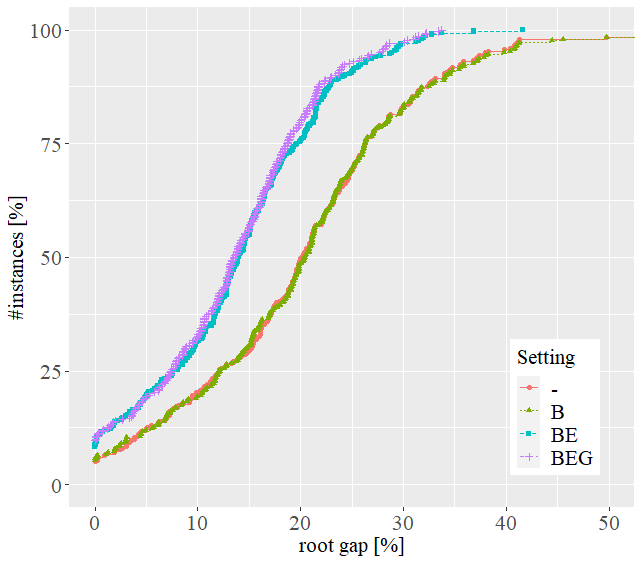
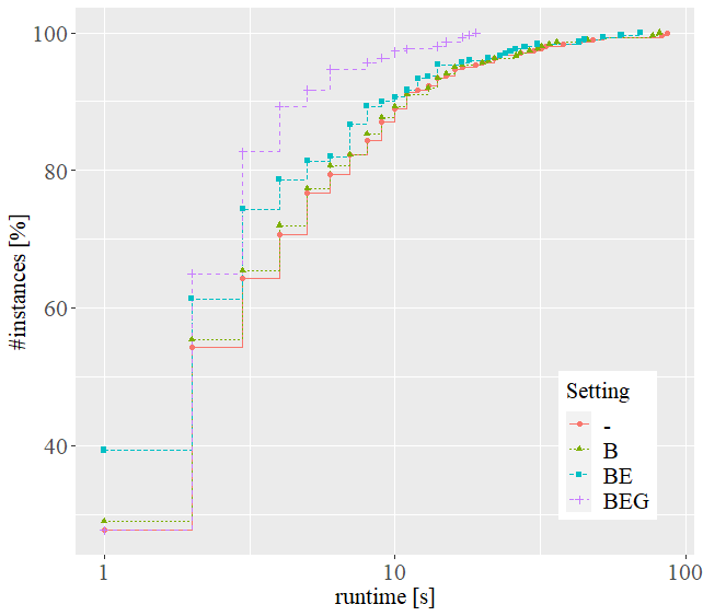
Figure 1: Root gaps and solution times of TRS data set instances.

5.1.3 CCLW Knapsack Interdiction Dataset

Our second benchmark for the KFG is derived from the instances proposed by Caprara et al., (2016) for the Knapsack Interdiction Problem. In this case too, we introduce an additional fortification level, and impose a cardinality constraint for the leader. For interdiction costs and budgets we used the data available in the original instances. The number of items takes value in $\{35,40,45,50,55\}$ and for each size there are ten instances in which the interdiction budget increases with the $ID$ of the instance, $1\leq ID\leq 10$. We solved these 50 instances for $B_{F}\in\{3,5\}$, thus producing a set of 100 benchmark instances denoted as CCLW.

Figure 2 shows the cumulative distribution of root gaps and solution times for the instances in this benchmark set. It can be seen that bound based strengthening does not have an effect in both measures. This is mostly due to the fact that we are able to produce only a few strengthened cuts, as the value of $\Phi(\hat{x})-\underline{z}$ is usually larger than $d_{i}$ in our experiments. Enumerative strengthening does not contribute to decreasing the solution times because of its time complexity, which depends on the interdiction budget; however this strategy decreases the root gap on average. Note that the root gap reduction is larger for smaller budget levels. We also observe smaller number of B&C nodes when enumerative strengthening is activated, although we do not report details about this kind of measure here. Similar to the results on the TRS data set, the most effective component regarding the solution time is greedy integer separation ($G$). We observe in our experiments that Algorithm 2 is able to find good interdiction strategies quickly, which makes the separation process more efficient compared to the default setting where we stop solving (SEP) once a violated fortification is found. We are able to solve 95 out of 100 instances optimally in one hour when using setting BEG.

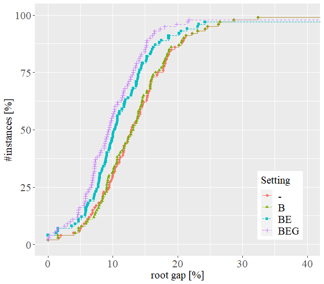
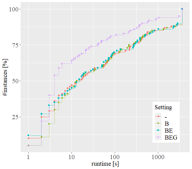
Figure 2: Root gaps and solution times of CCLW data set instances.

5.2 Results for the SPFG

In the following, we first describe problem specific implementation details of the B&C algorithm for the SPFG. Then, we present the results of our experiments on two existing data sets from the literature.

5.2.1 Implementation Details for the SPFG

The recourse problem, which is the shortest path problem, is solved via Dijkstra’s algorithm (Dijkstra et al.,, 1959) with a priority queue implementation, wherever needed, e.g., in Algorithm 2 and Algorithm 3. While solving (SEP) to obtain a fortification cut, both integer and fractional solutions are separated exactly. Separation is carried out in $O(|A|\log|V|)$ time. In addition to the lower cutoff and solution limit strategies, interdiction cut strengthening is used to speed up the solution of (SEP). Recall that any value $l>\theta^{*}$ can be used to lift the interdiction cut. Since all the problem parameters are integers in out data sets, we choose $l=\lceil\theta^{*}+\epsilon\rceil$. Remind that fortifying two assets (i.e., arcs) at the same time can be more effective than the sum of their individual effects only if the two arcs can be used together in a recourse solution (see Section 3.3). Accordingly, while executing Algorithm 3, we try to not consider all sets $P$ including pairs of arcs that cannot appear together in an $s-t$ path. Since checking this exactly would be time consuming, we only check if any two arcs in $P$ have the same head or tail and skip the current iteration if there is such an arc pair, which indicates that an $s-t$ path cannot include both of these arcs.

5.2.2 Directed Grid Networks

Table 1: The sizes of the grid networks.

Instance	Nodes	Arcs
10x10	102	416
20x20	402	1,826
30x30	902	4,236
40x40	1,602	7,646
50x50	2,502	12,056
60x60	3,602	17,466

For the SPFG, the first data set we use is the directed grid network instance set generated by Lozano and Smith, (2017) following the topology used by Israeli and Wood, (2002) and Cappanera and Scaparra, (2011). These instances and the implementation of the solution algorithm proposed in Lozano and Smith, (2017) are available at https://doi.org/10.1287/ijoc.2016.0721. In these networks, in addition to a source and a sink node, there are $m\times n$ nodes forming a grid with $m$ rows and $n$ columns. The source (sink) node is linked with each of the grid nodes in the first (last) column. The sizes of the networks are shown in Table 1. We use the cost ($c_{ij}$) and delay ($d_{ij}$) values provided with the networks, which were generated randomly in $[1,c_{max}]$ and $[1,d_{max}]$, respectively, using six different $c_{max}$ and $d_{max}$ combinations. For each network size, ten instances with different arc costs/delays are generated. Each instance is solved for six different fortification and interdiction budget level configurations $(B_{F},B_{I})$ also used in Lozano and Smith, (2017).

In Figure 3 the cumulative distributions of root gaps and solution times are plotted for three settings: the basic one “-”, the best performing setting for KFG instances (BEG), and a variant additionally considering interdiction cut strengthening (IBEG). The plot on the left hand side shows that the root gaps of variant BEG are substantially smaller than those of the basic setting. It is also clear from the plots that the strengthening of interdiction cuts using $l=\lceil\theta^{*}+\epsilon\rceil$ produces a remarkable improvement. We observed that, using this strategy the number of B&C nodes increased with respect to BEG, since attacker solutions with smaller objective values (and, in turn, weaker fortification cuts) are produced. Nevertheless, in this case, the separation problem can be solved extremely efficiently, which overall leads to improved performances.

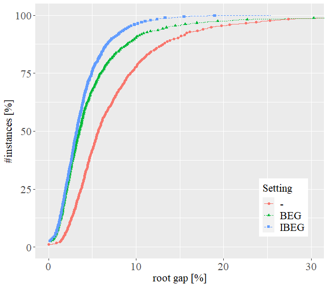
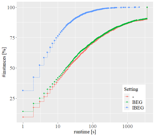
Figure 3: Root gaps and solution times of Grid networks data set.

Tables 2 and 3 report the average and maximum solution times required by our algorithm with setting IBEG. These figures are compared with the results obtained by the solution algorithm of Lozano and Smith, (2017), denoted as LS. Since the implementation of this algorithm is available online, we were able to run it on the same hardware as our algorithm. The algorithm was coded in Java and we ran it with Gurobi 9.2 as MIP solver. In both tables, rows are associated to a network size and a configuration for the fortification and interdiction budget levels, whereas the three blocks of columns refer to different cost-delay configurations $(c_{max}\mbox{-}d_{max})$, i.e., (10-5), (10-10), and (10-20) in Table 2; (100-50), (100-100), and (100-200) in Table 3.

Table 2: SPFG Solution Times for the Directed Grid Networks with Setting IBEG and with algorithm LS (Part 1).

			(10-5)				(10-10)				(10-20)
			IBEG		LS		IBEG		LS		IBEG		LS
	$B_{F}$	$B_{I}$	Avg	Max	Avg	Max	Avg	Max	Avg	Max	Avg	Max	Avg	Max
10x10	3	3	0.1	0.1	0.1	0.2	0.1	0.1	0.1	0.2	0.1	0.1	0.1	0.2
	4	3	0.1	0.1	0.1	0.3	0.1	0.2	0.2	0.2	0.1	0.1	0.2	0.2
	3	4	0.1	0.2	0.2	0.3	0.2	0.2	0.3	0.4	0.2	0.2	0.3	0.6
	5	4	0.2	0.2	0.3	0.5	0.2	0.3	0.4	0.5	0.2	0.4	0.4	0.6
	4	5	0.2	0.3	0.4	0.7	0.2	0.3	0.6	1.0	0.3	0.4	0.7	1.5
	7	5	0.3	0.6	1.1	1.7	0.4	0.6	1.1	1.5	0.6	1.0	1.3	1.9
20x20	3	3	0.3	0.5	0.4	1.0	0.3	0.6	0.6	2.1	0.3	0.8	0.6	2.6
	4	3	0.3	0.5	0.5	1.0	0.4	0.8	0.7	2.5	0.4	0.9	0.7	2.7
	3	4	0.4	1.0	0.6	1.3	0.4	0.8	1.0	2.5	0.5	0.8	1.2	5.2
	5	4	0.6	1.4	0.9	1.8	0.8	1.8	1.5	5.1	0.7	1.4	1.7	7.3
	4	5	0.8	1.2	2.1	5.6	0.9	1.6	2.7	9.9	0.9	1.4	3.0	11.4
	7	5	1.7	3.3	3.3	5.9	2.4	3.4	5.1	16.7	2.6	3.9	7.1	31.5
30x30	3	3	0.6	1.0	0.9	1.2	0.6	1.2	1.4	3.8	0.6	1.0	3.6	19.0
	4	3	0.6	0.9	1.1	1.8	0.8	1.3	1.8	4.6	0.8	1.2	3.9	19.6
	3	4	1.2	1.8	1.9	2.7	1.4	2.9	5.6	27.7	1.4	3.1	8.0	35.1
	5	4	1.9	3.4	2.7	3.9	2.1	3.1	5.8	16.4	2.0	2.9	9.2	35.9
	4	5	2.7	4.9	6.4	9.9	2.9	5.9	19.2	110.5	3.4	8.7	21.5	108.7
	7	5	5.6	9.7	12.3	24.5	7.2	13.8	29.2	146.2	7.6	12.8	28.0	115.1
40x40	3	3	1.7	3.5	2.7	6.0	1.8	4.3	5.4	26.9	1.8	4.3	7.8	43.3
	4	3	1.9	3.0	3.6	7.3	2.4	4.6	6.8	32.9	2.2	3.8	9.0	45.6
	3	4	2.7	5.1	3.9	6.3	3.3	8.2	37.4	267.9	3.3	9.3	63.6	540.0
	5	4	4.9	8.4	9.1	30.5	5.3	12.3	42.2	260.8	5.9	14.4	69.9	549.6
	4	5	6.0	11.3	13.7	33.4	10.5	38.8	247.3	1943.5	9.5	30.9	377.7	2786.6
	7	5	15.6	32.4	26.5	76.0	22.9	66.8	486.4	3514.0	27.9	124.1	516.7	4106.4
50x50	3	3	2.1	3.4	4.4	11.1	2.1	4.2	10.7	38.0	2.2	4.7	13.3	41.6
	4	3	2.8	6.8	6.6	25.2	2.8	5.0	19.7	82.2	2.7	5.3	14.4	45.4
	3	4	3.3	8.1	13.1	83.7	5.0	11.8	53.4	240.4	4.8	17.0	52.5	371.5
	5	4	5.9	9.6	15.8	87.6	7.6	20.2	112.9	627.1	8.5	28.1	61.1	416.2
	4	5	9.5	24.0	38.6	276.0	17.7	75.9	219.6	1068.9	14.6	67.5	112.6	858.0
	7	5	24.8	45.9	77.9	518.4	33.5	124.3	407.3	2325.3	38.1	149.2	102.3	624.7
60x60	3	3	4.0	8.1	11.4	30.4	4.4	7.4	21.8	65.6	4.1	6.4	32.0	73.7
	4	3	5.4	13.1	12.6	33.9	5.9	13.3	32.7	143.7	6.1	18.2	38.0	95.8
	3	4	7.1	13.9	15.1	28.2	10.5	18.1	69.6	299.4	11.1	23.3	95.0	426.7
	5	4	12.7	27.9	21.2	54.8	16.7	30.6	134.4	905.8	16.6	28.8	115.8	575.2
	4	5	18.8	26.3	40.5	76.6	35.5	107.3	285.4	915.7	30.4	75.1	265.7	1056.2
	7	5	45.7	80.6	108.6	351.8	87.0	185.0	624.8	3440.4	74.2	127.9	474.1	2155.0

Table 2 contains the results for smallest three cost-delay configurations, and shows that IBEG yields significantly smaller average and maximum solution times for most of the instances. In 104 (107) out of 108 configurations, IBEG produces a strictly smaller average (maximum) solution time. For many instances of larger sizes our algorithm is faster than LS by one order of magnitude. Overall, the performance improvement of IBEG over LS becomes more pronounced as the $c_{max}$ and $d_{max}$ values increase.

Table 3: SPFG Solution Times for the Directed Grid Networks with Setting IBEG and with algorithm LS (Part 2).

			(100-50)				(100-100)				(100-200)
			IBEG		LS		IBEG		LS		IBEG		LS
	$B_{F}$	$B_{I}$	Avg	Max	Avg	Max	Avg	Max	Avg	Max	Avg	Max	Avg	Max
10x10	3	3	0.1	0.2	0.1	0.2	0.3	0.4	0.2	0.3	0.1	0.2	0.2	0.2
	4	3	0.2	0.2	0.2	0.2	0.2	0.2	0.2	0.3	0.2	0.3	0.2	0.3
	3	4	0.3	0.4	0.3	0.5	0.2	0.4	0.4	0.6	0.3	0.4	0.4	0.9
	5	4	0.3	0.4	0.4	0.5	0.3	0.7	0.5	0.8	0.3	0.5	0.5	0.9
	4	5	0.4	0.5	0.8	1.3	0.5	0.7	1.0	2.0	0.6	0.9	1.1	2.4
	7	5	0.5	1.0	1.3	2.4	0.8	1.2	1.7	3.3	0.9	1.7	1.9	3.4
20x20	3	3	0.5	0.8	0.7	1.9	0.5	0.7	0.7	1.1	0.5	0.9	0.7	1.5
	4	3	0.6	0.9	0.9	1.7	0.6	1.1	0.8	1.2	0.7	1.2	0.8	1.7
	3	4	1.0	1.5	2.1	5.4	1.0	1.3	1.8	4.4	0.9	1.6	1.8	4.6
	5	4	1.7	3.1	2.6	4.8	1.8	3.0	2.4	6.1	1.7	3.3	2.4	5.7
	4	5	2.4	3.4	5.8	14.5	2.7	4.7	7.7	22.6	2.4	4.5	7.8	25.2
	7	5	6.3	9.6	7.7	12.3	5.9	8.9	9.4	22.9	5.5	8.7	9.5	28.7
30x30	3	3	1.2	2.3	2.9	17.5	1.5	3.1	1.9	4.0	1.3	2.2	2.4	6.0
	4	3	1.4	2.9	2.1	9.5	1.7	2.9	2.7	6.8	1.6	2.5	2.7	6.8
	3	4	2.5	5.1	4.6	13.7	2.3	3.3	5.1	14.7	2.4	3.4	4.8	10.8
	5	4	5.1	12.7	7.3	22.3	4.0	7.2	7.6	24.0	3.9	6.1	7.1	22.6
	4	5	6.7	10.0	19.0	97.4	6.0	10.1	22.3	52.6	6.3	10.8	19.6	75.3
	7	5	19.8	47.5	29.9	89.2	16.1	23.4	49.1	218.1	16.1	23.8	42.6	175.1
40x40	3	3	2.3	4.3	3.4	6.7	2.8	4.5	6.9	31.0	2.4	3.6	6.1	18.9
	4	3	3.0	3.9	4.1	6.6	3.2	7.0	9.3	53.3	3.2	7.3	7.5	23.7
	3	4	6.6	11.8	11.3	37.0	6.1	13.9	14.9	40.1	4.9	9.0	13.0	21.0
	5	4	11.0	22.7	16.3	50.3	10.0	18.6	27.2	137.6	8.6	14.4	22.4	85.4
	4	5	21.3	49.9	32.5	78.3	22.9	92.3	75.2	277.6	13.7	33.1	44.9	138.1
	7	5	56.8	95.1	53.0	128.1	57.9	144.5	157.2	934.0	50.4	174.6	114.4	705.3
50x50	3	3	4.3	10.1	10.0	33.0	5.6	18.4	36.4	234.9	5.2	19.4	40.5	182.0
	4	3	5.6	12.4	10.1	27.5	6.0	17.3	49.5	359.1	6.2	23.3	40.8	173.8
	3	4	12.9	37.0	28.7	98.3	15.0	42.9	108.8	763.7	9.5	25.8	76.2	268.2
	5	4	27.3	89.4	61.1	204.3	26.6	102.6	417.3	3678.8	20.0	52.2	104.7	496.7
	4	5	57.3	206.9	120.4	494.4	69.4	251.0	253.2	1436.7	58.5	227.9	309.5	1545.9
	7	5	281.0	1097.6	238.5	1099.6	135.7	402.5	912.6	7746.5	93.4	334.8	469.2	3025.0
60x60	3	3	8.2	25.0	14.0	40.9	9.2	28.2	52.1	338.1	8.3	22.0	62.3	250.7
	4	3	11.4	24.4	17.6	58.2	11.4	34.7	76.2	552.1	12.9	41.9	68.4	297.4
	3	4	21.2	33.8	44.9	92.0	25.7	104.6	260.6	1790.4	23.2	99.1	180.7	866.1
	5	4	45.5	169.6	64.9	194.8	52.7	246.0	254.0	1726.6	33.1	110.1	202.4	1029.8
	4	5	92.5	365.0	148.2	391.5	167.4	854.4	1281.5	7442.6	222.9	1677.1	1120.4	5620.4
	7	5	271.8	761.7	329.8	1325.5	368.6	1608.8	1256.7	6658.2	364.7	2149.1	1493.8	8691.8

Table 3 gives results for the largest cost-delay configurations. For these instances, again IBEG outperforms LS for most of the instances. Here, in 100 (103) out of 108 configurations, IBEG produces a strictly smaller average (maximum) solution time. As the instances get more difficult, IBEG becomes more advantageous. For the most difficult group of instances with $n=60$ and $(c_{max}-d_{max})$ is (100-100) or (100-200), the average solution times with IBEG are 80% and 78% smaller, respectively, than their LS counterparts. Moreover, IBEG solves all instances within the time limit of one hour.

5.2.3 Real Road Networks

Table 4: Results for instance set road network.

					IBEG			LS
Instance	Nodes	Arcs	$B_{F}$	$B_{I}$	Avg(s.)	Max(s.)	Solved	Avg(s.)	Max(s.)	Solved
DC	9559	39377	3	3	9.5	15.1	9	35.0	99.2	9
			4	3	14.2	29.4	9	39.9	101.8	9
			3	4	18.1	32.2	9	94.2	453.7	9
			5	4	45.3	68.4	9	104.0	426.5	9
			4	5	51.5	86.3	9	523.6	2959.7	9
			7	5	123.7	230.7	9	608.4	2126.0	9
RI	53658	192084	3	3	88.2	234.2	9	137.7	588.3	9
			4	3	164.3	289.3	9	144.2	570.1	9
			3	4	285.7	960.1	9	463.6	3031.8	9
			5	4	389.0	1432.8	9	465.4	2621.2	9
			4	5	1084.4	5766.4	9	1896.3	13758.4	9
			7	5	1565.7	6042.8	9	2092.1	TL	8
NJ	330386	1202458	3	3	858.3	1997.3	9	988.5	5442.5	9
			4	3	1078.8	2906.5	9	2057.4	TL	8
			3	4	1576.3	2849.0	9	2217.3	TL	8
			5	4	2968.8	8052.1	9	2557.4	TL	8
			4	5	5695.8	TL	8	2702.0	TL	8
			7	5	10042.3	TL	7	3885.4	TL	8
Total							159			156

For the second part of the SPFG experiments, we considered the real road network data sets of the cities Washington (DC), Rhode Island (RI), and New Jersey (NJ), used by Raith and Ehrgott, (2009) and Lozano and Smith, (2017). While the original undirected data sets are available at http://www.diag.uniroma1.it//~challenge9/data/tiger/, we used the data sets provided by Lozano and Smith, (2017) where each edge is replaced by two arcs to get directed networks and in which connectivity is enforced by additional high-cost arcs. The costs of the arcs are equal to the distances and the delay is 10 000 for each arc. On each of the three networks, the SPFG is solved for nine distinct $s-t$ pairs and using the six fortification and interdiction budget combinations used for the grid networks, resulting in 162 instances. As these are the most challenging instances considered in our study, the time limit is set to four hours for each run. Table 4 reports the sizes of the networks as well as average and maximum solution times over the nine instances with the same size and budget combination for IBEG and LS, as reported in Lozano and Smith, (2017). The table shows that our default setting IBEG is able to solve 159 over 162 instances optimally within the time limit. Notice that our B&C algorithm solves three instances more than the sampling based algorithm by Lozano and Smith, (2017), which was run on the same machine as IBEG and produced significantly smaller solution times than the ones reported in their paper. In addition, when both algorithms solve all the instances, IBEG is significantly faster than LS: the average computing time and the maximum computing times are below 48% and 72% on the average, respectively, of their counterpart for LS.

6 Conclusion

In this study we address fortification games (FGs), i.e., defender-attacker-defender problems which involve fortification, interdiction and recourse decisions, respectively. These problems are interesting from a theoretical viewpoint and have many real-world applications, in, e.g., military operations or the design of robust networks. We introduce fortification cuts, which allow for a single-level exact reformulation of this complex trilevel optimization problem, and a solution approach which uses the cuts within a branch-and-cut algorithm and works in the space of the fortification variables only.

While mainly focusing on the version where interdicting an asset depreciates its usefulness for the defender, we also show that our methodology is directly applicable to FGs with complete destruction of interdicted assets. After introducing the basic fortification cuts, we present two strengthening procedures that can be used to produce stronger inequalities, and give a detailed description of the separation procedure. We provide numerical results for two relevant test-cases, namely knapsack fortification games and shortest path fortification games. Due to the different structures and computational complexity of their recourse problems, we observe different effects of our algorithmic components in our computational study, and try to give insight about possible reasons.

Finally, we point out that our solution scheme is generic, and it leaves space for problem specific improvements. For example, for a given FG, one could solve the associated separation problem by means of a state-of-the-art exact method or using some specialized heuristic instead of the greedy method proposed in this paper. Moreover, problem-specific valid inequalities or strengthening procedures of the fortification cuts could also be possible.

References

- Akgün et al., (2011) Akgün, I., Tansel, B. c., and Wood, R. K. (2011). The multi-terminal maximum-flow network-interdiction problem. European Journal of Operational Research, 211(2):241–251.
- Alderson et al., (2011) Alderson, D. L., Brown, G. G., Carlyle, W. M., and Wood, R. K. (2011). Solving defender-attacker-defender models for infrastructure defense. Technical report, Naval Postgraduate School Monterey CA Dept Of Operations Research.
- Assimakopoulos, (1987) Assimakopoulos, N. (1987). A network interdiction model for hospital infection control. Computers in Biology and Medicine, 17(6):413–422.
- Baggio et al., (2021) Baggio, A., Carvalho, M., Lodi, A., and Tramontani, A. (2021). Multilevel approaches for the critical node problem. Operations Research, 69(2):486–508.
- Brown et al., (2006) Brown, G., Carlyle, M., Salmerón, J., and Wood, K. (2006). Defending critical infrastructure. Interfaces, 36(6):530–544.
- Cappanera and Scaparra, (2011) Cappanera, P. and Scaparra, M. P. (2011). Optimal allocation of protective resources in shortest-path networks. Transportation Science, 45(1):64–80.
- Caprara et al., (2014) Caprara, A., Carvalho, M., Lodi, A., and Woeginger, G. J. (2014). A study on the computational complexity of the bilevel knapsack problem. SIAM Journal on Optimization, 24(2):823–838.
- Caprara et al., (2016) Caprara, A., Carvalho, M., Lodi, A., and Woeginger, G. J. (2016). Bilevel knapsack with interdiction constraints. INFORMS Journal on Computing, 28(2):319–333.
- Church and Scaparra, (2007) Church, R. L. and Scaparra, M. P. (2007). Protecting critical assets: the r-interdiction median problem with fortification. Geographical Analysis, 39(2):129–146.
- Cochran et al., (2011) Cochran, J. J., Cox, L. A., Keskinocak, P., Kharoufeh, J. P., Smith, J. C., and Wood, R. K. (2011). Bilevel network interdiction models: Formulations and solutions. Wiley Encyclopedia of Operations Research and Management Science.
- Della Croce and Scatamacchia, (2020) Della Croce, F. and Scatamacchia, R. (2020). An exact approach for the bilevel knapsack problem with interdiction constraints and extensions. Mathematical Programming, 183(1):249–281.
- Dijkstra et al., (1959) Dijkstra, E. W. et al. (1959). A note on two problems in connexion with graphs. Numerische Mathematik, 1(1):269–271.
- Fakhry et al., (2021) Fakhry, R., Hassini, E., Ezzeldin, M., and El-Dakhakhni, W. (2021). Tri-level mixed-binary linear programming: Solution approaches and application in defending critical infrastructure. European Journal of Operational Research.
- Fischetti et al., (2017) Fischetti, M., Ljubić, I., Monaci, M., and Sinnl, M. (2017). A new general-purpose algorithm for mixed-integer bilevel linear programs. Operations Research, 65(6):1615–1637.
- Fischetti et al., (2018) Fischetti, M., Ljubić, I., Monaci, M., and Sinnl, M. (2018). On the use of intersection cuts for bilevel optimization. Mathematical Programming, 172(1-2):77–103.
- Fischetti et al., (2019) Fischetti, M., Ljubić, I., Monaci, M., and Sinnl, M. (2019). Interdiction games and monotonicity, with application to knapsack problems. INFORMS Journal on Computing, 31(2):390–410.
- Furini et al., (2020) Furini, F., Ljubić, I., Malaguti, E., and Paronuzzi, P. (2020). On integer and bilevel formulations for the -vertex cut problem. Mathematical Programming Computation, 12:133–164.
- (18) Furini, F., Ljubić, I., Malaguti, E., and Paronuzzi, P. (2021a). Casting light on the hidden bilevel combinatorial structure of the capacitated vertex separator problem. Operations Research. to appear.
- Furini et al., (2019) Furini, F., Ljubić, I., Martin, S., and Segundo, P. S. (2019). The maximum clique interdiction problem. European Journal of Operational Research, 277(1):112–127.
- (20) Furini, F., Ljubić, I., Segundo, P. S., and Zhao, Y. (2021b). A branch-and-cut algorithm for the edge interdiction clique problem. European Journal of Operational Research, 294(1):54–69.
- Israeli, (1999) Israeli, E. (1999). System Interdiction and Defense. PhD thesis, Operations Research Department, Naval Postgraduate School Monterey CA.
- Israeli and Wood, (2002) Israeli, E. and Wood, R. K. (2002). Shortest-path network interdiction. Networks: An International Journal, 40(2):97–111.
- Jin et al., (2015) Jin, J. G., Lu, L., Sun, L., and Yin, J. (2015). Optimal allocation of protective resources in urban rail transit networks against intentional attacks. Transportation Research Part E: Logistics and Transportation Review, 84:73–87.
- Kellerer et al., (2004) Kellerer, H., Pferschy, U., and Pisinger, D. (2004). Knapsack Problems. Springer, Berlin, Germany.
- Kleinert et al., (2021) Kleinert, T., Labbé, M., Ljubić, I., and Schmidt, M. (2021). A survey on mixed-integer programming techniques in bilevel optimization. EURO Journal on Computational Optimization, 9:100007.
- Lai et al., (2019) Lai, K., Illindala, M., and Subramaniam, K. (2019). A tri-level optimization model to mitigate coordinated attacks on electric power systems in a cyber-physical environment. Applied Energy, 235:204–218.
- Lim and Smith, (2007) Lim, C. and Smith, J. C. (2007). Algorithms for discrete and continuous multicommodity flow network interdiction problems. IIE Transactions, 39(1):15–26.
- Lodi et al., (2014) Lodi, A., Ralphs, T. K., and Woeginger, G. J. (2014). Bilevel programming and the separation problem. Mathematical Programming, 146(1):437–458.
- Lozano and Smith, (2017) Lozano, L. and Smith, J. C. (2017). A backward sampling framework for interdiction problems with fortification. INFORMS Journal on Computing, 29(1):123–139.
- Martello et al., (1999) Martello, S., Pisinger, D., and Toth, P. (1999). Dynamic programming and strong bounds for the 0-1 knapsack problem. Management Science, 3:414–424.
- Nabli et al., (2020) Nabli, A., Carvalho, M., and Hosteins, P. (2020). Complexity of the multilevel critical node problem. arXiv preprint arXiv:2007.02370.
- Raith and Ehrgott, (2009) Raith, A. and Ehrgott, M. (2009). A comparison of solution strategies for biobjective shortest path problems. Computers & Operations Research, 36(4):1299–1331.
- Sarhadi et al., (2017) Sarhadi, H., Tulett, D. M., and Verma, M. (2017). An analytical approach to the protection planning of a rail intermodal terminal network. European Journal of Operational Research, 257(2):511–525.
- (34) Scaparra, M. P. and Church, R. L. (2008a). A bilevel mixed-integer program for critical infrastructure protection planning. Computers & Operations Research, 35(6):1905–1923.
- (35) Scaparra, M. P. and Church, R. L. (2008b). An exact solution approach for the interdiction median problem with fortification. European Journal of Operational Research, 189(1):76–92.
- Shen et al., (2012) Shen, S., Smith, J. C., and Goli, R. (2012). Exact interdiction models and algorithms for disconnecting networks via node deletions. Discrete Optimization, 9(3):172–188.
- Smith and Lim, (2008) Smith, J. C. and Lim, C. (2008). Algorithms for network interdiction and fortification games. In Pareto optimality, game theory and equilibria, pages 609–644. Springer.
- Smith et al., (2007) Smith, J. C., Lim, C., and Sudargho, F. (2007). Survivable network design under optimal and heuristic interdiction scenarios. Journal of Global Optimization, 38(2):181–199.
- Smith and Song, (2020) Smith, J. C. and Song, Y. (2020). A survey of network interdiction models and algorithms. European Journal of Operational Research, 283(3):797–811.
- Starita and Scaparra, (2016) Starita, S. and Scaparra, M. P. (2016). Optimizing dynamic investment decisions for railway systems protection. European Journal of Operational Research, 248(2):543–557.
- Starita et al., (2017) Starita, S., Scaparra, M. P., and O’Hanley, J. R. (2017). A dynamic model for road protection against flooding. Journal of the Operational Research Society, 68(1):74–88.
- Tahernejad et al., (2020) Tahernejad, S., Ralphs, T. K., and DeNegre, S. T. (2020). A branch-and-cut algorithm for mixed integer bilevel linear optimization problems and its implementation. Mathematical Programming Computation, 12(4):529–568.
- Tang et al., (2016) Tang, Y., Richard, J.-P. P., and Smith, J. C. (2016). A class of algorithms for mixed-integer bilevel min–max optimization. Journal of Global Optimization, 66(2):225–262.
- Tanınmış et al., (2021) Tanınmış, K., Aras, N., and Altınel, İ. K. (2021). Improved x-space algorithm for min-max bilevel problems with an application to misinformation spread in social networks. European Journal of Operational Research, 297(1):40–52.
- Wang et al., (2016) Wang, Z., Yin, Y., and An, B. (2016). Computing optimal monitoring strategy for detecting terrorist plots. In Schuurmans, D. and Wellman, M. P., editors, Proceedings of the Thirtieth AAAI Conference on Artificial Intelligence, February 12-17, 2016, Phoenix, Arizona, USA, pages 637–643. AAAI Press.
- Xiang and Wang, (2018) Xiang, Y. and Wang, L. (2018). An improved defender–attacker–defender model for transmission line defense considering offensive resource uncertainties. IEEE Transactions on Smart Grid, 10(3):2534–2546.
- Yuan et al., (2014) Yuan, W., Zhao, L., and Zeng, B. (2014). Optimal power grid protection through a defender–attacker–defender model. Reliability Engineering & System Safety, 121:83–89.
- Zheng and Albert, (2018) Zheng, K. and Albert, L. A. (2018). An exact algorithm for solving the bilevel facility interdiction and fortification problem. Operations Research Letters, 46(6):573–578.