Subaru High-$z$ Exploration of Low-Luminosity Quasars (SHELLQs). XVI. 69 New Quasars at $5.8<z<7.0$

Abstract

We present the spectroscopic discovery of 69 quasars at $5.8<z<7.0$, drawn from the Hyper Suprime-Cam (HSC) Subaru Strategic Program (SSP) imaging survey data. This is the 16th publication from the Subaru High-$z$ Exploration of Low-Luminosity Quasars (SHELLQs) project, and completes identification of all but the faintest candidates (i.e., $i$-band dropouts with $z_{\rm AB}<24$ and $y$-band detections, and $z$-band dropouts with $y_{\rm AB}<24$) with Bayesian quasar probability $P_{\rm Q}^{\rm B}>0.1$ in the HSC-SSP third public data release (PDR3). The sample reported here also includes three quasars with $P_{\rm Q}^{\rm B}<0.1$ at $z\sim 6.6$, which we selected in an effort to completely cover the reddest point sources with simple color cuts. The number of high-$z$ quasars discovered in SHELLQs has now grown to 162, including 23 type-II quasar candidates. This paper also presents identification of seven galaxies at $5.6<z<6.7$, an [O III] emitter at $z=0.954$, and 31 Galactic cool stars and brown dwarfs. High-$z$ quasars and galaxies comprise 75 % and 16 % respectively of all the spectroscopic SHELLQs objects that pass our latest selection algorithm with the PDR3 photometry. That is, a total of 91 % of the objects lie at $z>5.6$. This demonstrates that the algorithm has very high efficiency, even though we are probing an unprecedentedly low-luminosity population down to $M_{1450}\sim-21$ mag.

1 Introduction

The astronomical community is making great strides toward charting and understanding quasars at the epoch of cosmic reionization, which is thought to have taken place during the interval $6<z<10$ (Planck Collaboration et al., 2020). Quasars at $5.7<z\leq 7.0$ have been discovered from optical wide-field ($>$100-deg² class) multi-band surveys, such as the Sloan Digital Sky Survey (SDSS; Fan et al., 2000, 2001, 2003, 2004, 2006; Jiang et al., 2008, 2009, 2015), the Canada-France-Hawaii Telescope Legacy Survey (CFHTLS; Willott et al., 2005, 2007, 2009, 2010a, 2010b), the Panoramic Survey Telescope And Rapid Response System 1 survey (Pan-STARRS1; Bañados et al., 2014, 2016; Venemans et al., 2015; Mazzucchelli et al., 2017), the Dark Energy Survey (DES; Reed et al., 2015, 2017, 2019; Yang et al., 2019), and the Dark Energy Spectroscopic Instrument Legacy Imaging Surveys (DELS; Wang et al., 2017, 2018, 2019). Near-infrared (IR) surveys are paving the way to probe more distant objects, and indeed quasars at $z>6.5$ have been detected with, e.g., the United Kingdom Infrared Telescope (UKIRT) Infrared Deep Sky Survey (Mortlock et al., 2011), the Visible and Infrared Survey Telescope for Astronomy (VISTA) Kilo-degree Infrared Galaxy Survey (VIKING; Venemans et al., 2013), and the UKIRT and VISTA Hemisphere Surveys, with three objects at $z=7.5-7.6$ marking the highest-redshift quasars currently known (Bañados et al., 2018; Yang et al., 2020; Wang et al., 2021). We will soon reach deeper into the epoch of reionization with the advent of Euclid and the Roman Space Telescope. These two space missions will provide unprecedentedly wide-and-deep maps of the near-IR sky, and are expected to identify quasars up to $z\sim 10$ (e.g., Euclid Collaboration et al., 2019). High-$z$ quasars thus discovered have been probing, and will further probe, the formation of the first supermassive black holes (SMBHs) and their host galaxies, the history and sources of reionization, and other key issues in the early universe.

We have been carrying out a high-$z$ quasar survey complementary to the existing ones for the past several years, going much deeper in relatively small areas of the sky. The project (“Subaru High-$z$ Exploration of Low-Luminosity Quasars”; SHELLQs) exploits the exquisite imaging data produced by the Hyper Suprime-Cam (HSC; Miyazaki et al., 2018) Subaru Strategic Program (SSP) survey. Three layers named Wide, Deep, and UltraDeep constitute the HSC-SSP survey, covering (1400, 26, 3.5) deg² down to 5$\sigma$ limiting magnitudes of $i_{\rm AB}$ = (25.9, 26.8, 27.4) for point sources, respectively (Aihara et al., 2018). Thus far we have reported spectroscopic identification of 93 low-luminosity quasars at $5.7<z<7.1$, including 18 type-II quasar candidates with very luminous and narrow Ly$\alpha$ emission, in a series of SHELLQs publications (Matsuoka et al., 2016, 2018a, 2018b, 2019a, 2019b). Follow-up near-IR spectroscopy has revealed that the quasars have a variety of accretion modes, from sub-Eddington accretion onto massive SMBHs to (super-)Eddington accretion onto less massive ones (Onoue et al., 2019, M. Onoue et al., in prep.). The host galaxies probed with ALMA are also diverse, sometimes accompanied by active star formation and powerful extended outflows (Izumi et al., 2021a, b), while their dynamical masses are more or less consistent with those inferred from the local mass relation between SMBHs and the host bulges (Izumi et al., 2018, 2019).

This is the 16th publication from the SHELLQs project, presenting the spectroscopic discovery of 69 new high-$z$ quasars accumulated over the past two years. The basics of candidate selection and spectroscopic observations are described in §2, followed by the results and discussion in §3. We use point-spread-function (PSF) magnitudes ($m_{\rm AB}$) and associated errors ($\sigma_{\rm m})$ presented in the AB system (Oke & Gunn, 1983) unless otherwise noted, corrected for Galactic extinction (Schlegel et al., 1998). We refer to $z$-band magnitudes with the AB subscript (“$z_{\rm AB}$”), while redshift $z$ appears without a subscript. The cosmological parameters are assumed to be $H_{0}$ = 70 km s^-1 Mpc^-1, $\Omega_{\rm M}$ = 0.3, and $\Omega_{\rm\Lambda}$ = 0.7.

2 Candidate selection and spectroscopy

Our candidate selection strategy remains mostly unchanged since the beginning of the project, and is detailed in our previous papers. Here, we itemize the essential steps, with an emphasis on recent updates.

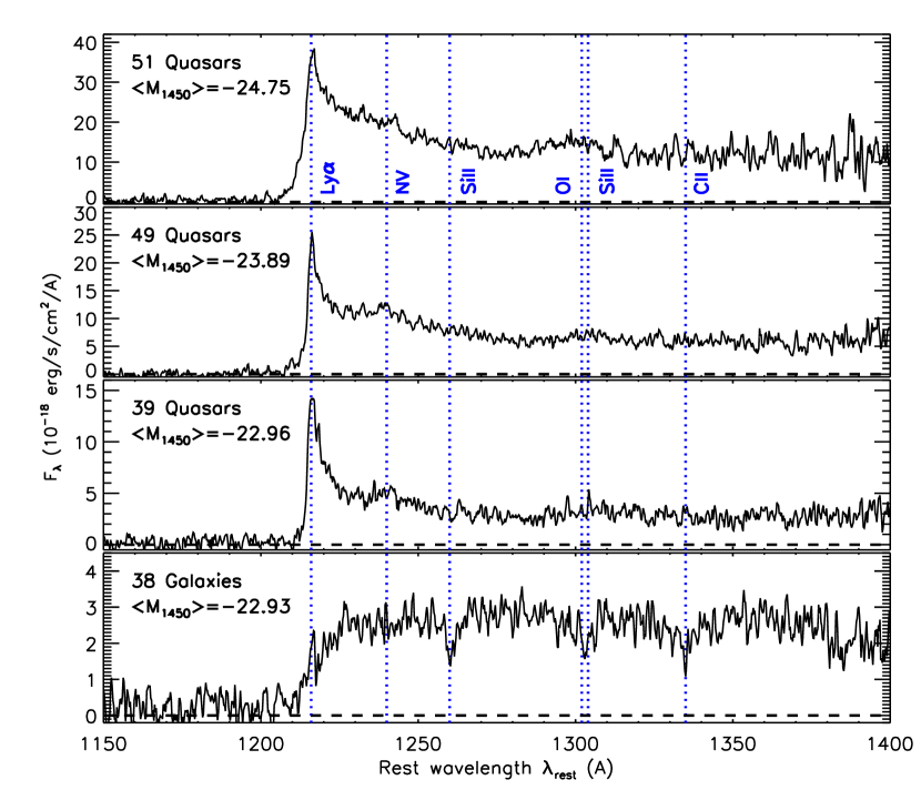
Figure 8: Median-stacked spectra of the high-$z$ objects discovered by SHELLQs. The top three panels present those created from 51 quasars with $M_{1450}<-24.2$, 49 quasars with $-23.5<M_{1450}<-24.2$, and 39 quasars with $M_{1450}>-23.5$, while the bottom panel presents that created from 38 galaxies. The median $M_{1450}$ of the stacked objects is reported in each panel.

1. We first select point sources meeting the criteria
   ($z_{\rm AB}<24.5$ & $\sigma_{z}<0.155$ & $i_{\rm AB}-z_{\rm AB}>1.5$) OR
   ($y_{\rm AB}<25.0$ & $\sigma_{y}<0.217$ & $z_{\rm AB}-y_{\rm AB}>0.8$)
   from the HSC-SSP database. The candidates selected with the first/second set of conditions are referred to as $i$-/$z$-dropouts in what follows. Our definition of “point sources” uses the ratio between the adaptive moment (Hirata & Seljak, 2003) of a given source ($\mu$; averaged over the two image dimensions) and that of the PSF model ($\mu_{\rm PSF}$). For $i$-dropouts, we use the cut $0.7<\mu/\mu_{\rm PSF}<1.2$ measured in the $z$-band. This criterion removes spectroscopic high-$z$ galaxies more efficiently than does the condition we previously used (i.e., requiring that the difference between the PSF and CModel magnitudes be less than 0.15), while retaining $>$90 % of the high-$z$ broad-line quasars we identified (see Figure 8 of Matsuoka et al., 2019a). A looser cut, $0.6<\mu/\mu_{\rm PSF}<3.0$ measured in the $y$-band, is used for $z$-dropouts, to be more inclusive. We exclude from the selection those sources with $g$- or $r$-band detections or any critical quality issues in the photometry, such as those caused by saturation, cosmic rays, bad pixels, and nearby bright stars. In addition, we eliminate the bluest candidates with $i_{\rm AB}-z_{\rm AB}<2.5$ and $z_{\rm AB}-y_{\rm AB}<-1.0$, as we have found that such sources are dominated by [O III] line emitters at $z\sim 0.8$ (see below).

2. The list of selected sources is matched to public near-IR survey catalogs. All the objects presented in this paper were found from the HSC-SSP Wide layer, where we use $Y$-, $J$-, $H$-, and $K$-band magnitudes measured with the UKIRT Wide-Field Camera (WFCAM; Casali et al., 2007) or the VISTA Infrared Camera (VIRCAM; Dalton et al., 2006). The data were obtained as a part of the UKIDSS Large Area Survey (available in the data release [DR] 11PLUS), the UKIDSS Hemisphere Survey (DR1), the VIKING (DR5), or the VISTA Hemisphere Survey (DR6). The entire HSC-SSP Wide layer is covered in at least one band of the above NIR surveys.

3. We calculate a Bayesian probability ($P_{\rm Q}^{\rm B}$) for each candidate being a high-$z$ quasar, following the recipe provided by Mortlock et al. (2012), using the matched HSC $i$-, $z$-, $y$-band and near-IR magnitudes. The calculation considers flux upper limits in the HSC bands, while near-IR magnitudes are used only when a source is detected in the given band. Our algorithm includes models of high-$z$ quasars and Galactic cool stars and brown dwarfs, taking into account their spectral energy distributions (SEDs) and surface densities as a function of apparent magnitude and Galactic coordinates. We select all the candidates with $P_{\rm Q}^{\rm B}>0.1$, and also keep a fraction of the remaining sources (the “low-$P_{\rm Q}^{\rm B}$ sample” hereafter; see below), for the subsequent selection.

4. All the pre-stacked and stacked images of the candidates are retrieved from the HSC-SSP database, and screened by an automatic algorithm based on Source Extractor (Bertin & Arnouts, 1996) and by visual inspection. This step removes numerous false detections missed by the catalog quality flags, such as cosmic rays and detector artifacts, as well as variable sources.

5. The candidates are fed into follow-up spectroscopy programs at the 8.2-m Subaru Telescope and the 10.4-m Gran Telescopio Canarias (GTC). We use the Faint Object Camera and Spectrograph (FOCAS; Kashikawa et al., 2002) on Subaru to observe the wavelength range 0.75 – 1.0 $\mu$m with the VPH900 grism and 1″.0 slits, giving a spectral resolution of $R\sim 1200$ (Program ID: S18B-011I). Similarly, the Optical System for Imaging and low-intermediate-Resolution Integrated Spectroscopy (OSIRIS; Cepa et al., 2000) on GTC is used with the R2500I grism and 1″.0 longslit, yielding spectra over 0.75 – 1.0 $\mu$m with $R\sim 1500$ (Program IDs: GTC5-20A, GTC10-20B, GTC42-21B). The objects presented in this paper were observed mostly in gray nights under both photometric and non-photometric sky conditions, with a typical seeing of 0″.6 – 1″.2.

We have so far completed spectroscopy of all but the faintest candidates drawn from $\sim$1200 deg² of the HSC-SSP public data release 3 (PDR3; Aihara et al., 2021). The remaining candidates are either (i) $i$-dropouts with $z_{\rm AB}>24.0$ or without $y$-band detections, or (ii) $i$-dropouts with $z_{\rm AB}>23.5$ and $i_{\rm AB}-z_{\rm AB}<2.0$. All the $z$-dropout candidates have been observed; while the formal magnitude cut is $y_{\rm AB}=25.0$ (Step 1), the actual limiting magnitude depends mostly on the depth achieved in the HSC imaging, which is $y_{\rm AB}\sim 24.4$ for 5$\sigma$ detection of point sources in the Wide layer (Aihara et al., 2021). This paper presents spectroscopic identification of 108 candidates, observed over the past two years since our previous discovery paper (Matsuoka et al., 2019a).

3 Results and Discussion

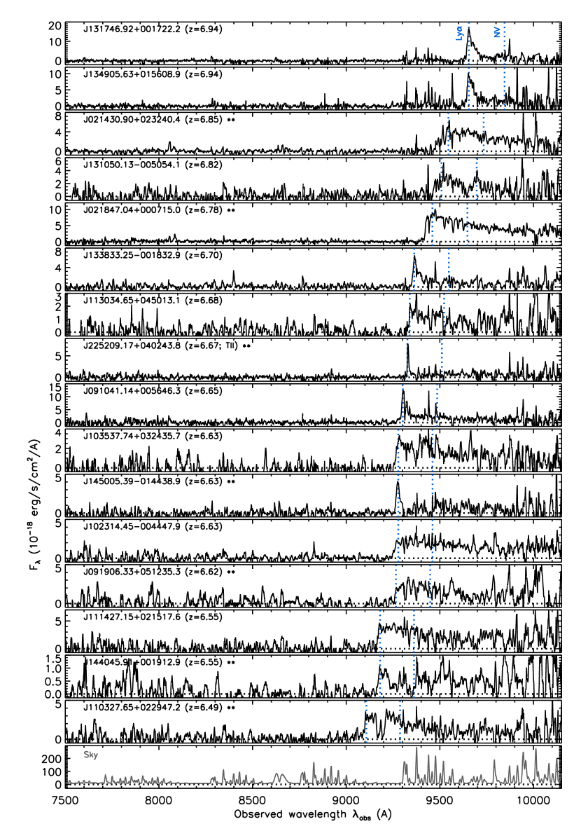
Figure 1: Discovery spectra of the first set of 16 quasars, displayed in decreasing order of redshift. The object name and the estimated redshift (with uncertainty $\Delta z\sim 0.01-0.1$; see text) are indicated at the top left corner of each panel, with the two asterisks indicating that the object is noted in the text. The five type-II quasar candidates are marked with “TII” adjacent to the redshifts. The blue dotted lines mark the expected positions of the Ly$\alpha$ and N V $\lambda$1240 emission lines, given the redshifts. The spectra were smoothed using inverse-variance weighted means over 3 – 13 pixels (depending on the signal-to-noise ratio [S/N]), for display purposes. The bottom panel displays a sky spectrum, as a guide to the expected noise.

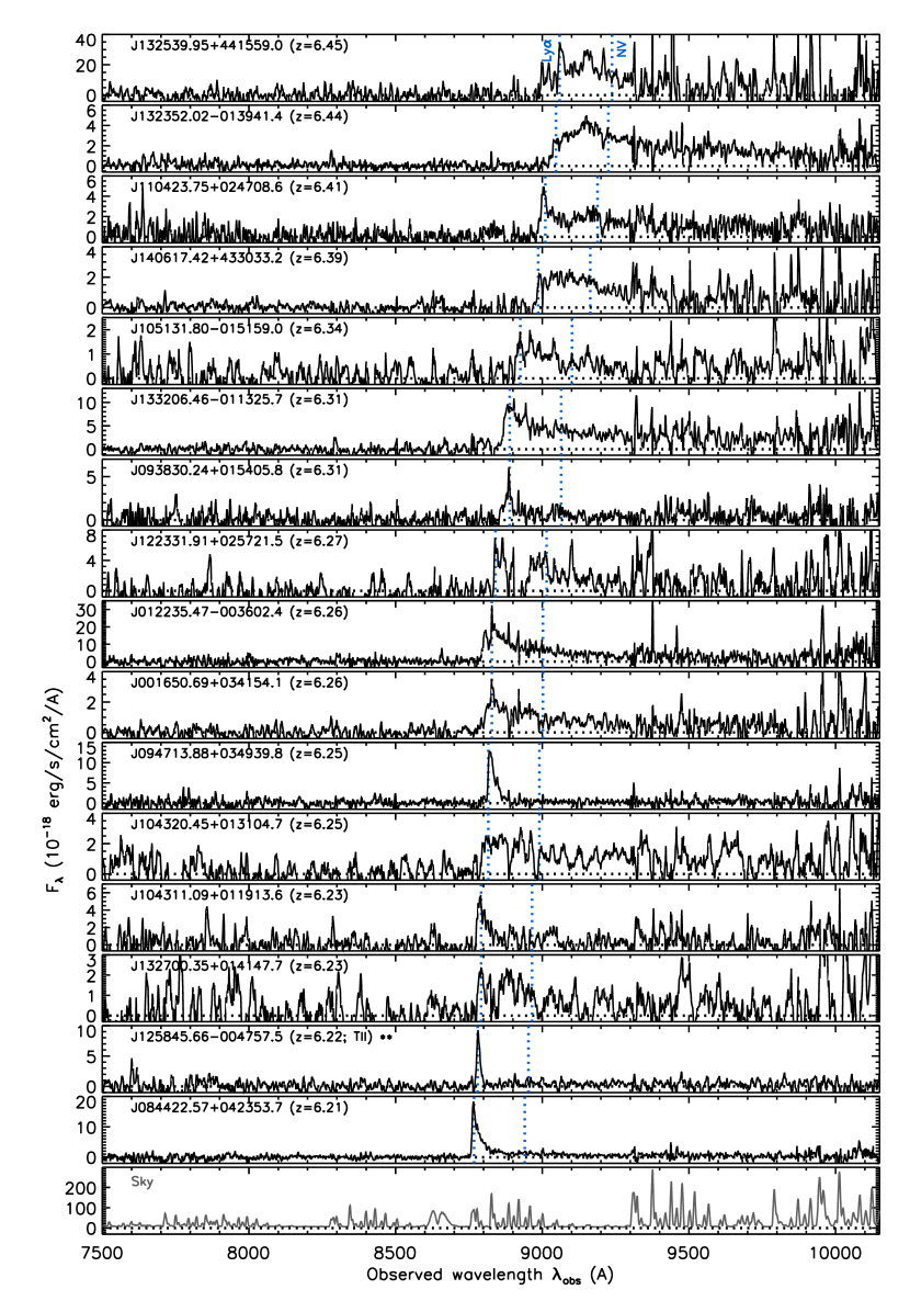
Figure 2: Same as Figure 1, but for the second set of 16 quasars.

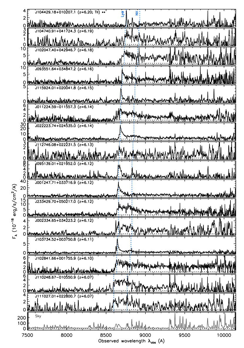
Figure 3: Same as Figure 1, but for the third set of 16 quasars.

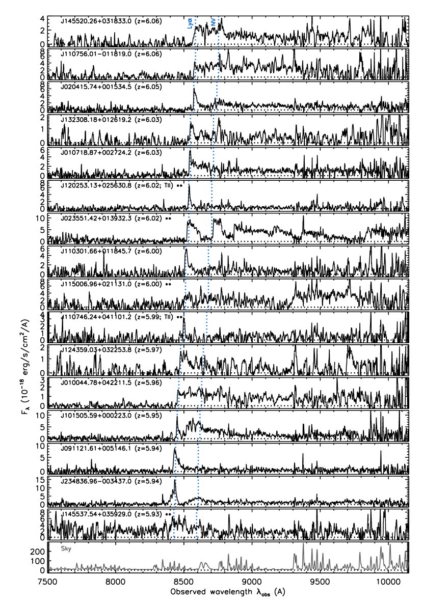
Figure 4: Same as Figure 1, but for the fourth set of 16 quasars.

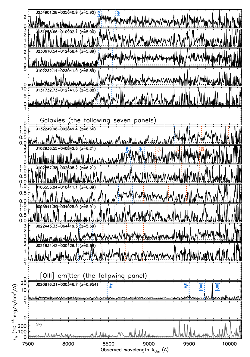
Figure 5: Same as Figure 1, but for the last set of quasars in the top five panels. The following panels present seven galaxies and an [O III] emitter, with the expected positions of Si II $\lambda$1260, Si II $\lambda$1304, and C II $\lambda$1335 (for the galaxies) and of H$\gamma$, H$\beta$, and [O III] $\lambda$4959, $\lambda$5007 lines (for the [O III] emitter) marked by the dotted lines.

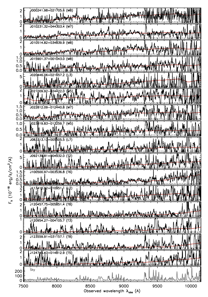
Figure 6: Same as Figure 1, but for the first set of 16 Galactic cool stars and brown dwarfs, ordered by the right ascension. The red lines represent the best-fit templates, whose spectral types are indicated at the top left corner of the individual panels.

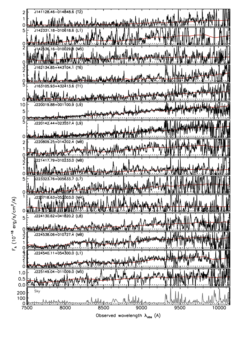
Figure 7: Same as Figure 6, but for the last set of 15 Galactic dwarfs.

Table 1 is the journal of discovery spectroscopy, including the coordinates and photometric information of the observed candidates. The objects detected in the near-IR bands are listed in Table 2. The 108 candidates include 69 quasars at $5.8<z<7.0$, seven galaxies at $5.6<z<6.7$, an [O III] emitter at $z=0.954$, and 31 cool stars and brown dwarfs in the Milky Way. Figures 1 – 7 present their reduced spectra, in the same order as in Table 1. The spectra have been scaled in flux to match the HSC magnitudes in the $z$/$y$ bands for $i$-/$z$-dropouts. We found clear trace of signals in both the 2d and 1d spectra of all the presented objects.

The classification and measurements of the spectra are performed in a way consistent with our previous papers. The 69 objects in Figures 1 – 5 (top panels) are classified as high-$z$ quasars based on the broad Ly$\alpha$ line, blue rest-frame ultraviolet continuum, and/or sharp continuum break just blueward of Ly$\alpha$. Seven high-$z$ objects lacking AGN signatures are classified as galaxies (Figure 5 middle panels). The 69 quasars include five type-II candidates ($J225209.17+040243.8$, $J125845.66-004757.5$, $J104429.18+010207.1$, $J120253.13+025630.8$, and $J110746.24+041101.2$) with very luminous ($>10^{43}$ erg s^-1) and narrow (full width at half maximum [FWHM] $<$ 500 km s^-1) Ly$\alpha$ emission. Such Ly$\alpha$ features are often associated with active galactic nuclei (AGNs) in the lower-$z$ Universe (e.g., Alexandroff et al., 2013; Konno et al., 2016; Sobral et al., 2018; Spinoso et al., 2020). Indeed, our deep Keck/MOSFIRE spectroscopy of a similar object from SHELLQs has revealed very strong C IV $\lambda$1549 doublet lines, demonstrating that it is an AGN (Onoue et al., 2021b). Past surveys of high-$z$ Ly$\alpha$ emitters (LAEs) also found similar objects at the bright end ($>10^{43}$ erg s^-1) of the Ly$\alpha$ luminosity function, with a significant contribution expected from AGNs (e.g., Santos et al., 2016; Konno et al., 2018). However, it is currently hard to make a clear distinction between extreme star formation, AGN, and other possibilities powering those most luminous LAEs; future observations in other wavelengths, in particular X-rays for AGNs, will be key to making robust classifications.

The distinction between the faint (type-I) quasars and galaxies is also sometimes ambiguous, partly due to the limited data quality. Figure 8 presents the composite spectra of the high-$z$ quasars in three bins of absolute magnitudes ($M_{1450}<-24.2$, $-24.2<M_{1450}<-23.5$, and $-23.5<M_{1450}$; type-II candidates were excluded) and of the high-$z$ galaxies, discovered in SHELLQs so far. These spectra were generated by moving the individual spectra to the rest frame, normalizing to the median $M_{1450}$ of each group of objects being stacked, and then median-stacking. The 39 quasars in the lowest luminosity bin and the 38 galaxies have similar distributions and median values of $M_{1450}$, but the composite spectra are strikingly different; the quasar composite shows clear broad emission lines of Ly$\alpha$ and N V $\lambda$1240, while the galaxy composite lacks such emission features and instead has interstellar absorption lines of Si II $\lambda$1260, Si II $\lambda$1304, and C II $\lambda$1335. This demonstrates that our spectral separation between quasars and galaxies is robust as a whole, while there may be minor cases of misclassification for individual objects.

We measured the redshift of each quasar or galaxy via the observed wavelength of the Ly$\alpha$ line or of the onset of the IGM H I absorption. This procedure is not always easy, due to the H I damping-wing absorption, the ambiguity in determining the onset of the Gunn & Peterson (1965, GP) trough, and low signal-to-noise (S/N) spectra in some cases. The uncertainty of the present redshift measurements is thus relatively large, from $\Delta z\sim 0.01$ (when Ly$\alpha$ has a clear peak) to $\sim 0.1$ (when Ly$\alpha$ emission is not visible). The absolute magnitude ($M_{1450}$) of each object was measured by extrapolating the observed luminosity in a continuum window, selected at wavelengths relatively free of strong sky emission lines, by assuming a power-law continuum model ($F_{\lambda}\propto\lambda^{\alpha}$) with $\alpha=-1.5$ for quasars (e.g., Vanden Berk et al., 2001) or $\alpha=-2.0$ for galaxies (e.g., Stanway et al., 2005). The Ly$\alpha$ ($+$ N V $\lambda$1240) properties were measured with the continuum flux estimated either on the red side of the line (for objects with relatively narrow Ly$\alpha$) or with the above power-law continuum model (for the remaining objects). Table 3 summarizes the results of the spectral measurements, and Figure 9 presents the distribution of redshifts and absolute magnitudes of all the SHELLQs objects at $z>5.6$, including those reported in our previous papers.

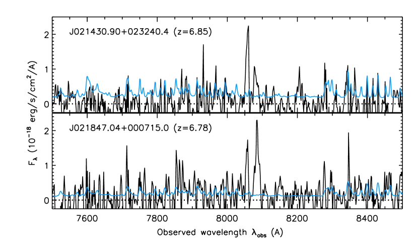
Figure 10: Examples of the transmitted fluxes in the GP trough, found along the sightlines toward J021430.90+023240.4 (top) and J021847.04+000715.0 (bottom). The black and cyan lines represent the observed fluxes and associated 1$\sigma$ errors, respectively.

Here we briefly note on a few quasars with unusual spectral features. $J115006.96+021131.0$ ($z=6.00$) has a second continuum break at $\lambda_{\rm obs}\simeq 9300$ Å. This break is also clear in the 2d spectra, and the HSC color of this object ($z_{\rm AB}-y_{\rm AB}=0.64$) is considerably redder than expected for a typical quasar at the same redshift (see Figure 11 below). No particular feature is known at the corresponding rest-frame wavelength ($\lambda_{\rm rest}\sim 1330$ Å) in a typical quasar spectrum (e.g., Vanden Berk et al., 2001), and thus the origin of this break is unclear. The HSC images show no evidence of an overlapping source; the quasar is a clear point source without significant displacement observed between the $i$-, $z$-, and $y$-band image centroids. Nonetheless, if the second break corresponds to the Ly$\alpha$ wavelength of a background source, its redshift would be $z\sim 6.6$. Alternatively, this feature might be caused by a broad absorption line (BAL) of Si II $\lambda$1398 with very high blueshift velocities, $>$15,000 km s^-1. $J023551.42+013932.3$ ($z=6.02$) exhibits unambiguous features of BALs; weaker absorption features may be present in other objects as well (e.g., $J110327.65+022947.2$ at $z=6.49$), but higher-quality data are necessary for the confirmation of their presence and nature, e.g., whether they are intrinsic to the quasars or are produced by foreground metal absorbers. $J145537.54+035929.0$ ($z=5.93$) has significant excess flux at $\lambda_{\rm obs}<8400$ Å  in the GP trough. This is surprising, since the HSC colors ($i_{\rm AB}-z_{\rm AB}=2.1$ and $z_{\rm AB}-y_{\rm AB}=-0.4$) are perfectly consistent with being a quasar at $z=5.9$. Indeed the color estimated from the spectrum, $i_{\rm AB}-z_{\rm AB}<0.6$, conflicts with the HSC measurement. This object is either (i) a high-$z$ quasar with an overlapping foreground transient source that appeared after the HSC imaging and affected only the spectroscopic observations, or (ii) a low-$z$ variable source (however, we are not aware of any similar spectra in the literature) which was relatively faint/bright at the time of the HSC $i$-/$z$-band imaging, making it appear to be an $i$-dropout in broad-band photometry. We tentatively keep this object in the quasar category for now, and will revisit its nature with future observations. Finally, while most of our low-luminosity quasars have no observable signal in the GP trough, the brightest ones sometimes exhibit spikes of transmitted flux. For example, $J021430.90+023240.4$ ($z=6.85$) and $J021847.04+000715.0$ ($z=6.78$) have significant positive signals at $\lambda_{\rm obs}=8050-8100$ Å as displayed in Figure 10; these signals are also apparent in the 2d spectra. The large numbers of low-luminosity quasars will offer a unique probe of the small-scale structure of reionization, once higher-quality spectra are obtained with future deep observations.

Figure 11 displays the two-color diagram of all 312 objects with spectroscopic identification reported in the past and present SHELLQs papers. The quasars populate the lower-right and upper portions of this diagram and are almost absent in between ($1<z_{\rm AB}-y_{\rm AB}<2$), where the quasar model track intersects the stellar and brown-dwarf sequence; sources with such moderate colors can exceed $P^{\rm B}_{\rm Q}=0.1$ only when they are very close to the quasar model track or have near-IR magnitudes that exclude the case of Galactic dwarfs. The HSC colors of the spectroscopically-confirmed galaxies are indistinguishable from those of the quasars, but most of the galaxies that we select are at $z\leq 6$. This is presumably related to the faintness of these galaxies, with magnitudes mostly around $z_{\rm AB}=24.0$, i.e., close to the limit of our follow-up spectroscopy. They would quickly become fainter if redshifted to $z>6$, as the observed $z$-band flux is progressively dominated by the GP trough.

The present quasar candidates also include an [O III] emitter at $z=0.954$, as displayed in Figure 5. The strong [O III] $\lambda$4959 and $\lambda$5007 lines in the $y$-band give this galaxy a red $z-y$ color. Table 3 reports the measurements of the two [O III] lines, H$\gamma$, and H$\beta$. Our past selection included many similar objects at $z\sim 0.8$, which appear as $i$-dropouts due to the strong lines in the $z$-band. We now know that their colors are distinct from those of high-$z$ quasars, as evident in Figure 11, and thus we recently incorporated an additional color cut ($i-z<2.5$ and $z-y<-1.0$, as mentioned in §2) which eliminates most such contaminants.

We have also identified 31 Galactic cool stars and brown dwarfs with the present spectroscopy, as displayed in Figures 6 and 7. Table 4 lists the rough spectral classes, estimated by fitting the spectral standard templates of M4- to T8-type dwarfs (Burgasser, 2014; Skrzypek et al., 2015) to the observed spectra. We emphasize that the stellar classifications are meant to be only approximate, given the relatively poor data quality and limited spectral coverage. The number of Galactic dwarfs identified in SHELLQs has now grown to 96, many of which entered the sample because of inaccurate HSC photometry in past DRs. Indeed, the majority of the dwarfs have $P^{\rm B}_{\rm Q}<0.1$ and thus would not be selected as candidates with the magnitudes from PDR3; see Figure 11. The HSC-SSP data reduction pipeline (hscPipe; Bosch et al., 2018) provides accurate flux measurements for the vast majority of sources, but the high-$z$ quasars we are seeking are as rare as the very unusual cases of erroneous photometry that happened to dwarfs. On a related note, the dwarfs we have identified spectroscopically represent a very biased sample, since the selection algorithm is tuned to remove typical dwarfs with correct photometry. Figure 11 indicates that only the dwarfs closest to the quasar model track have $P^{\rm B}_{\rm Q}>0.1$, as one would expect. Finally, given the limited data quality, we cannot exclude the possibility that some of these objects actually belong to extragalactic populations, e.g., compact and quiescent galaxies at $z\sim 1$ which have similar colors to Galactic dwarfs; a further investigation on this issue requires much deeper observations than presented here.

The above tables and figures include 16 objects from our first set of spectroscopy of the low-$P^{\rm B}_{\rm Q}$ sample, which are deliberately selected from the sources with $P^{\rm B}_{\rm Q}<0.1$ (see Step 3 of the selection flow in §2). Together with the main spectroscopic program for the $P^{\rm B}_{\rm Q}>0.1$ candidates, these additional observations have completed the identification of PDR3 point sources with ($z_{\rm AB}<24.0$, $\sigma_{z}<0.155$, $i_{\rm AB}-z_{\rm AB}>2.0$, $z_{\rm AB}-y_{\rm AB}<0.5$, and $y$-band detection; $i$-dropouts) across the entire Wide layer, and those with ($y_{\rm AB}<24.0$, $\sigma_{y}<0.155$, and $z_{\rm AB}-y_{\rm AB}>2.0$; $z$-dropouts) in the Spring fields (RA = 8^h – 17^h) of the Wide layer. We found that the 16 targets include three quasars at $z=6.55-6.63$ ($J091906.33+051235.3$, $J144045.91+001912.9$, and $J145005.39-014438.9$) and 13 Galactic dwarfs. The redshift $z=6.6$ corresponds to the quasar color $z_{\rm AB}-y_{\rm AB}\sim 2.0$, a boundary between the $P^{\rm B}_{\rm Q}>0.1$ and $<0.1$ regions of the two-color diagram (Figure 11), so discovery of the three quasars is perfectly consistent with what one would expect. We see no evidence of significant incompleteness in the Bayesian selection compared to the simple color cuts.

As previously mentioned, a significant fraction of the contaminants in our spectroscopic sample comes from inaccurate HSC photometry in earlier DRs. A number of factors have contributed to the continuous improvement of the photometry, including the additional exposures of the same fields and the updated algorithms of hscPipe for better treatments of, e.g., sky subtraction, removal of scattered light and artifacts, photometric calibration, and object detection (Bosch et al., 2018; Aihara et al., 2019, 2021). If we had started the SHELLQs project with PDR3 photometry, the success rate of follow-up spectroscopy would have been much higher. Out of the 312 spectroscopically-identified objects plotted in Figure 11, 205 pass our latest selection with the PDR3 photometry. Of the 205 objects, 154 are high-$z$ quasars (including 22 type-II candidates) and 33 are galaxies, amounting to fractions of 75 % (64 % if the type-II candidates are excluded) and 16 %, respectively. Thus 91 % of the photometric candidates lie at $z>5.6$. The [O III] emitters make a negligible contribution (3 objects, 1 %), while the contamination rate of Galactic dwarfs is 7 % (15 objects). Thus our selection algorithm has very high efficiency, even though we are probing an unprecedentedly low-luminosity population of quasars.

We are approaching the end of the HSC-SSP survey; as of Nov 2021, the survey has observed for 325 of the allocated 330 nights. PDR3 includes the reduced data from 278 nights, and the spectroscopic identification of all but the faintest high-$z$ quasar candidates from the data have been reported in the previous and present SHELLQs papers. The remaining candidates will be covered in our forthcoming observations, and eventually, an SSP survey planned with the Subaru Prime Focus Spectrograph (PFS) under development (Takada et al., 2014; Tamura et al., 2016, 2018) will provide the opportunity to observe a broader range of candidates, e.g., very faint ($z_{\rm AB}>24.5$) or extended $i$-dropouts. We aim to start the PFS-SSP survey in 2023.

The new discoveries reported here represent a significant increase in the size of the SHELLQs sample. Our next goals are to tighten the constraints on the luminosity function (LF) at $z=6$ (Matsuoka et al., 2018c) and measure the LF at $z=7$. Diverse follow-up projects are also ongoing, including near-zone size measurements (e.g., Ishimoto et al., 2020, T.-Y. Lu et al., in prep.), clustering analyses, and characterization of the optical discovery spectra (A. Takahashi et al., in prep.) and near-IR broadband SEDs (e.g., Kato et al., 2020), as well as the two key projects with near-IR spectrographs and ALMA described in §1. Further ambitious programs have been approved and await observations, including those with Chandra and James Webb Space Telescope (Onoue et al., 2021a) to study SHELLQs objects in greater detail.

Figure 9: Redshifts and the rest-frame ultraviolet absolute magnitudes ($M_{1450}$) of all the high-$z$ objects reported in the past and present SHELLQs papers, including quasars (blue dots), type-II quasar candidates (blue dots enclosed by larger circles), and galaxies (green dots). We also plot all the other high-$z$ quasars published to date (gray dots), compiled mostly from the papers referenced in §1.

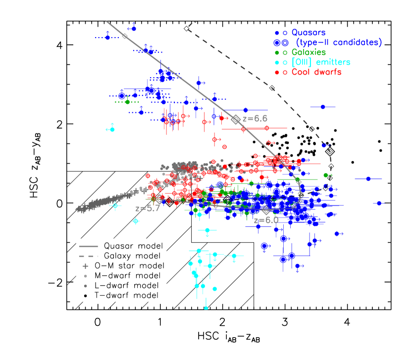
Figure 11: HSC $i-z$ and $z-y$ colors of the high-$z$ quasars (blue symbols), the high-$z$ galaxies (green), the [O III] emitters at $z=0.8-1.0$ (cyan), and Galactic cool stars and brown dwarfs (red), with spectroscopic identification reported in the past and present SHELLQs papers; the filled and open circles represent those with $P_{\rm Q}^{\rm B}>0.1$ and $P_{\rm Q}^{\rm B}\leq 0.1$, respectively. The magnitudes are taken from PDR3. The arrows represent 3$\sigma$ limits, while the objects detected only in the $y$-band are placed at $i_{\rm AB}-z_{\rm AB}=i_{\rm AB}^{\rm lim}-z_{\rm AB}^{\rm lim}$ with dotted error bars, where $m_{\rm AB}^{\rm lim}$ represents the 3$\sigma$ limiting magnitude. We also plot the model colors of quasars (solid curve) and galaxies (dashed curve) at $z\geq 5.7$, with the diamonds marking redshifts at $\Delta z=0.1$ intervals. The gray crosses and dots represent simulated colors of main-sequence stars and M-, L-, T-type brown dwarfs, as indicated at the bottom-left corner (see Matsuoka et al., 2016, for the details of those models). The hatched area represents the color cuts used in Step 1 of the selection (see §2).

Table 1: Journal of Discovery Spectroscopy

Object	$i_{\rm AB}$	$z_{\rm AB}$	$y_{\rm AB}$	$P_{\rm Q}^{\rm B}$	$t_{\rm exp}$	Date (Inst)
	(mag)	(mag)	(mag)		(min)
Quasars
$J131746.92+001722.2$	$>$26.02	$>$24.77	22.22 $\pm$ 0.03	1.000	120	2020 Apr 25 & 30 (O)
$J134905.63+015608.9$	$>$26.00	$>$24.27	22.20 $\pm$ 0.07	1.000	120	2020 Mar 4 & Apr 25 (O)
$J021430.90+023240.4$	26.41 $\pm$ 0.44	$>$25.49	21.86 $\pm$ 0.02	1.000	120	2020 Sep 17 – 18 (O)
$J131050.13-005054.1$	27.06 $\pm$ 0.48	$>$25.16	22.55 $\pm$ 0.04	1.000	35	2021 Feb 21 (F)
$J021847.04+000715.0$	26.08 $\pm$ 0.23	$>$24.82	21.10 $\pm$ 0.01	1.000	50	2019 Oct 4 – 6 (F)
$J133833.25-001832.9$	26.40 $\pm$ 0.29	25.61 $\pm$ 0.24	22.72 $\pm$ 0.04	1.000	30	2020 Dec 22 (F)
$J113034.65+045013.1$	27.71 $\pm$ 0.88	26.00 $\pm$ 0.68	22.78 $\pm$ 0.05	0.972	25	2021 Jan 5 (F)
$J225209.17+040243.8$	26.65 $\pm$ 0.54	25.89 $\pm$ 0.38	23.12 $\pm$ 0.08	0.403	30	2019 Oct 4 (F)
$J091041.14+005646.3$	26.78 $\pm$ 0.35	24.41 $\pm$ 0.06	22.06 $\pm$ 0.02	1.000	15	2020 Dec 22 (F)
$J103537.74+032435.7$	$>$25.88	24.99 $\pm$ 0.24	22.60 $\pm$ 0.05	0.111	30	2021 Jan 3 (F)
$J145005.39-014438.9$	$>$26.27	25.67 $\pm$ 0.28	23.45 $\pm$ 0.08	0.003	30	2021 Feb 21 (F)
$J102314.45-004447.9$	$>$26.10	25.11 $\pm$ 0.17	22.08 $\pm$ 0.02	1.000	15	2020 Dec 22 (F)
$J091906.33+051235.3$	26.83 $\pm$ 0.57	24.47 $\pm$ 0.21	22.28 $\pm$ 0.05	0.027	15	2021 Feb 22 (F)
$J111427.15+021517.6$	27.20 $\pm$ 0.44	23.36 $\pm$ 0.04	21.91 $\pm$ 0.02	1.000	15	2021 Jan 4 (F)
$J144045.91+001912.9$	27.12 $\pm$ 0.55	25.46 $\pm$ 0.21	23.39 $\pm$ 0.06	0.006	60	2021 Feb 23 & Mar 3 (F)
$J110327.65+022947.2$	$>$25.97	23.39 $\pm$ 0.04	22.51 $\pm$ 0.07	0.910	15	2021 Jan 4 (F)
$J132539.95+441559.0$	25.42 $\pm$ 0.10	20.91 $\pm$ 0.01	20.92 $\pm$ 0.01	1.000	5	2021 Aug 16 (O)
$J132352.02-013941.4$	25.79 $\pm$ 0.27	22.85 $\pm$ 0.03	21.93 $\pm$ 0.03	1.000	30	2020 Mar 3 (O)
$J110423.75+024708.6$	27.13 $\pm$ 0.57	23.18 $\pm$ 0.03	22.94 $\pm$ 0.08	1.000	10	2021 Jan 4 (F)
$J140617.42+433033.2$	$>$25.36	23.43 $\pm$ 0.04	23.46 $\pm$ 0.15	1.000	90	2021 Aug 12 (O)
$J105131.80-015159.0$	$>$26.00	23.79 $\pm$ 0.06	23.35 $\pm$ 0.11	1.000	30	2021 Jan 4 (F)
$J133206.46-011325.7$	24.94 $\pm$ 0.09	21.87 $\pm$ 0.01	21.53 $\pm$ 0.02	1.000	15	2020 Apr 30 (O)
$J093830.24+015405.8$	26.99 $\pm$ 0.42	23.82 $\pm$ 0.06	23.55 $\pm$ 0.10	1.000	30	2021 Jan 3 (F)
$J122331.91+025721.5$	26.00 $\pm$ 0.15	22.86 $\pm$ 0.03	22.77 $\pm$ 0.04	1.000	30	2020 Mar 3 (O)
$J012235.47-003602.4$	24.40 $\pm$ 0.07	21.14 $\pm$ 0.01	21.35 $\pm$ 0.01	1.000	15	2020 Sep 18 (O)
$J001650.69+034154.1$	27.04 $\pm$ 0.61	23.33 $\pm$ 0.04	23.32 $\pm$ 0.06	1.000	90	2021 Aug 2 (O)
$J094713.88+034939.8$	27.12 $\pm$ 0.54	23.20 $\pm$ 0.04	24.15 $\pm$ 0.18	1.000	15	2021 Jan 3 (F)
$J104320.45+013104.7$	26.95 $\pm$ 0.50	22.94 $\pm$ 0.02	22.52 $\pm$ 0.04	1.000	25	2021 Feb 20 (F)
$J104311.09+011913.6$	26.25 $\pm$ 0.25	23.70 $\pm$ 0.03	23.85 $\pm$ 0.13	1.000	30	2021 Feb 20 (F)
$J132700.35+014147.7$	26.75 $\pm$ 0.53	23.50 $\pm$ 0.05	23.37 $\pm$ 0.08	1.000	35	2021 Jan 3 (F)
$J125845.66-004757.5$	27.32 $\pm$ 0.70	23.72 $\pm$ 0.05	23.55 $\pm$ 0.11	1.000	20	2021 Jan 2 (F)
$J084422.57+042353.7$	26.01 $\pm$ 0.25	22.61 $\pm$ 0.02	23.10 $\pm$ 0.10	1.000	15	2020 Dec 22 (F)
$J104429.18+010207.1$	26.91 $\pm$ 0.38	24.11 $\pm$ 0.04	24.13 $\pm$ 0.17	1.000	25	2021 Mar 3 (F)
$J104740.91+041724.3$	26.63 $\pm$ 0.26	23.09 $\pm$ 0.02	23.02 $\pm$ 0.07	1.000	15	2021 Jan 5 (F)
$J102047.40+042946.7$	25.15 $\pm$ 0.09	21.64 $\pm$ 0.01	21.29 $\pm$ 0.01	1.000	15	2020 Nov 18 (O)
$J093551.64+034847.2$	25.28 $\pm$ 0.08	22.24 $\pm$ 0.01	22.26 $\pm$ 0.03	1.000	15	2020 Nov 18 (O)
$J115924.01+020041.8$	27.11 $\pm$ 0.47	23.97 $\pm$ 0.06	24.64 $\pm$ 0.19	1.000	30	2021 Feb 20 (F)
$J011224.59-011557.3$	25.33 $\pm$ 0.27	22.38 $\pm$ 0.07	22.39 $\pm$ 0.04	1.000	90	2020 Dec 24 (F)
$J022223.74+024535.0$	24.72 $\pm$ 0.15	21.44 $\pm$ 0.01	21.82 $\pm$ 0.03	1.000	10	2020 Dec 22 (F)
$J112746.08+022231.5$	26.40 $\pm$ 0.22	23.41 $\pm$ 0.04	23.28 $\pm$ 0.08	1.000	30	2021 Jan 5 (F)
$J095139.01+021952.0$	$>$26.19	23.54 $\pm$ 0.05	25.79 $\pm$ 0.66	1.000	15	2021 Feb 21 (F)
$J001247.71+033716.9$	25.10 $\pm$ 0.10	21.37 $\pm$ 0.01	21.65 $\pm$ 0.01	1.000	15	2021 Aug 1 (O)
$J233429.70+050217.0$	24.68 $\pm$ 0.11	21.46 $\pm$ 0.02	21.57 $\pm$ 0.04	1.000	15	2021 Aug 1 (O)
$J002334.65+034223.2$	25.91 $\pm$ 0.19	22.82 $\pm$ 0.02	22.80 $\pm$ 0.04	1.000	30	2021 Aug 2 (O)
$J103734.52+003750.8$	26.38 $\pm$ 0.27	23.29 $\pm$ 0.04	23.66 $\pm$ 0.12	1.000	60	2020 Mar 3 (O)
$J102841.66+001755.9$	24.84 $\pm$ 0.07	21.87 $\pm$ 0.01	21.72 $\pm$ 0.02	1.000	15	2021 Feb 21 (F)
$J110248.67-010550.9$	25.05 $\pm$ 0.07	22.30 $\pm$ 0.01	22.37 $\pm$ 0.03	1.000	15	2021 Jan 24 (O)
$J111027.01+022800.7$	26.31 $\pm$ 0.25	22.69 $\pm$ 0.02	22.76 $\pm$ 0.06	1.000	15	2021 Jan 4 (F)
$J145520.26+031833.0$	25.75 $\pm$ 0.18	22.55 $\pm$ 0.02	22.60 $\pm$ 0.05	1.000	25	2021 Feb 20 (F)
$J110756.01-011819.0$	24.52 $\pm$ 0.04	21.77 $\pm$ 0.01	21.62 $\pm$ 0.02	1.000	15	2021 Jan 23 (O)
$J020415.74+001534.5$	25.42 $\pm$ 0.12	22.58 $\pm$ 0.02	22.78 $\pm$ 0.04	1.000	20	2020 Dec 22 (F)
$J132308.18+012619.2$	$>$25.45	23.80 $\pm$ 0.07	23.94 $\pm$ 0.14	1.000	20	2021 Jan 3 (F)
$J010718.87+002724.2$	25.12 $\pm$ 0.09	22.56 $\pm$ 0.03	22.58 $\pm$ 0.03	1.000	15	2019 Oct 4 (F)
$J120253.13+025630.8$	26.20 $\pm$ 0.17	23.66 $\pm$ 0.06	23.77 $\pm$ 0.10	1.000	15	2021 Feb 20 (F)
$J023551.42+013932.3$	24.46 $\pm$ 0.07	21.30 $\pm$ 0.01	21.48 $\pm$ 0.02	1.000	10	2020 Dec 22 (F)
$J110301.66+011845.7$	24.84 $\pm$ 0.07	22.92 $\pm$ 0.02	22.88 $\pm$ 0.06	1.000	15	2021 Feb 21 (F)
$J115006.96+021131.0$	24.52 $\pm$ 0.05	22.25 $\pm$ 0.02	21.61 $\pm$ 0.01	1.000	30	2021 Jan 2 (F)
$J110746.24+041101.2$	26.19 $\pm$ 0.20	24.02 $\pm$ 0.06	23.87 $\pm$ 0.14	0.994	25	2021 Mar 3 (F)
$J124359.03+032253.8$	26.24 $\pm$ 0.26	23.88 $\pm$ 0.06	23.89 $\pm$ 0.08	1.000	25	2021 Feb 21 (F)
$J010044.78+042211.5$	25.13 $\pm$ 0.15	22.96 $\pm$ 0.02	23.09 $\pm$ 0.07	1.000	45	2021 Aug 11 (O)
$J101505.59+000223.0$	24.04 $\pm$ 0.03	21.85 $\pm$ 0.01	22.15 $\pm$ 0.08	1.000	15	2021 Jan 24 (O)
$J091121.61+005146.1$	25.03 $\pm$ 0.07	23.30 $\pm$ 0.03	23.33 $\pm$ 0.05	1.000	25	2020 Dec 23 (F)
$J234836.96-003437.0$	23.88 $\pm$ 0.03	22.39 $\pm$ 0.02	22.65 $\pm$ 0.04	1.000	15	2019 Oct 5 (F)
$J145537.54+035929.0$	24.23 $\pm$ 0.06	22.15 $\pm$ 0.02	22.52 $\pm$ 0.05	1.000	25	2021 Feb 20 (F)
$J234901.28+005640.9$	24.40 $\pm$ 0.04	22.85 $\pm$ 0.02	22.82 $\pm$ 0.05	1.000	40	2020 Dec 22 (F)
$J131258.66+010902.1$	25.13 $\pm$ 0.12	22.98 $\pm$ 0.04	22.90 $\pm$ 0.09	1.000	15	2021 Jan 2 (F)
$J230610.54-012458.4$	24.62 $\pm$ 0.08	22.80 $\pm$ 0.04	22.41 $\pm$ 0.07	0.020	15	2019 Oct 5 (F)
$J102232.14+023041.9$	24.46 $\pm$ 0.06	22.64 $\pm$ 0.03	22.56 $\pm$ 0.07	1.000	15	2021 Jan 4 (F)
$J131732.73+012741.6$	23.70 $\pm$ 0.03	22.14 $\pm$ 0.02	22.09 $\pm$ 0.02	1.000	15	2020 May 16 (O)
Galaxies
$J132249.98+002849.4$	$>$25.89	$>$25.39	23.40 $\pm$ 0.08	1.000	50	2021 Feb 21 (F)
$J102936.55+040842.6$	26.36 $\pm$ 0.32	23.16 $\pm$ 0.04	22.57 $\pm$ 0.04	1.000	25	2021 Jan 3 (F)
$J102257.38-002608.2$	26.13 $\pm$ 0.25	24.01 $\pm$ 0.08	24.01 $\pm$ 0.14	0.912	25	2021 Mar 2 (F)
$J103553.04-010411.1$	26.69 $\pm$ 0.42	24.15 $\pm$ 0.07	24.30 $\pm$ 0.18	1.000	25	2021 Mar 3 (F)
$J095541.39+034025.0$	26.21 $\pm$ 0.23	24.09 $\pm$ 0.06	24.30 $\pm$ 0.16	1.000	25	2021 Mar 2 (F)
$J022443.33-064419.3$	24.96 $\pm$ 0.10	23.26 $\pm$ 0.05	23.02 $\pm$ 0.10	0.322	25	2019 Oct 5 (F)
$J021834.42-000426.1$	25.17 $\pm$ 0.10	23.81 $\pm$ 0.07	23.73 $\pm$ 0.09	0.381	30	2019 Oct 5 (F)
[O III] Emitter
$J020816.31+000346.7$	25.68 $\pm$ 0.18	$>$24.89	23.59 $\pm$ 0.07	0.105	10	2019 Oct 5 (F)
Cool Dwarfs
$J000241.98+021705.6$	25.15 $\pm$ 0.08	22.97 $\pm$ 0.05	22.72 $\pm$ 0.09	1.000	45	2020 Sep 19 (O)
$J010231.32+044303.4$	25.29 $\pm$ 0.46	23.28 $\pm$ 0.05	23.21 $\pm$ 0.12	0.830	90	2021 Aug 3 (O)
$J010514.82+034839.9$	$>$25.09	23.36 $\pm$ 0.05	22.79 $\pm$ 0.06	1.000	90	2021 Aug 12 (O)
$J015901.37+001043.0$	25.41 $\pm$ 0.10	24.01 $\pm$ 0.08	23.69 $\pm$ 0.07	0.000	60	2019 Oct 6 (F)
$J020446.06+021657.2$	24.51 $\pm$ 0.05	22.96 $\pm$ 0.03	22.72 $\pm$ 0.05	0.620	45	2020 Sep 20 (O)
$J021009.92-024422.0$	25.12 $\pm$ 0.04	23.16 $\pm$ 0.04	22.95 $\pm$ 0.05	1.000	25	2021 Jan 5 (F)
$J022812.09-012440.8$	$\cdots$	23.62 $\pm$ 0.04	23.24 $\pm$ 0.07	1.000	120	2020 Oct 10 (O)
$J023819.83-013259.7$	25.87 $\pm$ 0.29	24.07 $\pm$ 0.08	23.93 $\pm$ 0.18	0.019	70	2019 Oct 5 – 6 (F)
$J083313.13+005505.5$	25.93 $\pm$ 0.38	23.82 $\pm$ 0.08	23.36 $\pm$ 0.10	0.000	75	2021 Feb 22 – 23 (F)
$J092139.81+004932.0$	24.52 $\pm$ 0.04	22.67 $\pm$ 0.02	21.63 $\pm$ 0.01	0.000	15	2021 Feb 20 (F)
$J100500.97+003536.8$	27.07 $\pm$ 0.38	25.04 $\pm$ 0.15	22.90 $\pm$ 0.06	0.114	40	2020 Dec 22 (F)
$J113410.92+010951.1$	24.73 $\pm$ 0.05	23.21 $\pm$ 0.03	23.18 $\pm$ 0.06	1.000	25	2021 Feb 21 (F)
$J120457.75+005851.4$	$>$26.35	25.61 $\pm$ 0.21	23.55 $\pm$ 0.08	0.000	25	2021 Mar 2 (F)
$J120954.27-004105.7$	$>$26.45	25.91 $\pm$ 0.30	23.86 $\pm$ 0.10	0.000	30	2021 Mar 2 (F)
$J123559.91+031157.1$	$>$25.90	25.39 $\pm$ 0.26	23.26 $\pm$ 0.05	0.000	50	2021 Feb 22 (F)
$J124746.47+014812.9$	$>$25.99	25.35 $\pm$ 0.20	23.33 $\pm$ 0.06	0.000	25	2021 Feb 23 (F)
$J141128.46-014848.6$	27.07 $\pm$ 0.51	25.34 $\pm$ 0.26	23.14 $\pm$ 0.05	0.000	60	2021 Feb 22 (F)
$J142331.18-010618.6$	24.05 $\pm$ 0.03	22.01 $\pm$ 0.01	21.10 $\pm$ 0.01	1.000	15	2020 Apr 24 (O)
$J142536.16-010029.8$	25.05 $\pm$ 0.07	23.37 $\pm$ 0.04	23.11 $\pm$ 0.06	0.925	15	2021 Feb 21 (F)
$J162134.85+443104.1$	$>$25.83	24.77 $\pm$ 0.24	22.72 $\pm$ 0.07	0.001	15	2021 Feb 23 (F)
$J163105.93+432413.6$	26.11 $\pm$ 0.13	22.89 $\pm$ 0.02	21.83 $\pm$ 0.02	0.994	15	2021 Feb 20 (F)
$J220019.88+001100.9$	23.41 $\pm$ 0.03	21.25 $\pm$ 0.01	20.65 $\pm$ 0.02	0.000	15	2020 Aug 20 (O)
$J220142.44+023557.4$	24.48 $\pm$ 0.06	22.60 $\pm$ 0.03	21.82 $\pm$ 0.03	0.000	30	2020 Aug 20 (O)
$J220809.25+014202.4$	24.77 $\pm$ 0.05	22.95 $\pm$ 0.02	22.61 $\pm$ 0.03	1.000	45	2020 Sep 20 (O)
$J221417.79+010233.0$	25.43 $\pm$ 0.08	23.41 $\pm$ 0.04	22.73 $\pm$ 0.04	0.000	10	2019 Oct 5 (F)
$J223323.76+005633.7$	24.13 $\pm$ 0.02	22.34 $\pm$ 0.01	21.56 $\pm$ 0.01	0.000	15	2020 Aug 28 (O)
$J223718.63+052003.0$	25.82 $\pm$ 0.25	24.18 $\pm$ 0.08	24.01 $\pm$ 0.13	0.001	50	2019 Oct 6 (F)
$J224130.62+041820.2$	23.85 $\pm$ 0.03	22.36 $\pm$ 0.01	21.56 $\pm$ 0.02	0.000	15	2020 Aug 24 (O)
$J224538.06+010727.4$	24.16 $\pm$ 0.03	22.61 $\pm$ 0.02	21.89 $\pm$ 0.02	0.000	30	2020 Aug 20 (O)
$J224540.11+054300.0$	24.17 $\pm$ 0.06	22.57 $\pm$ 0.02	21.98 $\pm$ 0.03	0.000	23	2020 Aug 20 (O)
$J225149.04-011009.0$	25.29 $\pm$ 0.18	23.42 $\pm$ 0.08	23.40 $\pm$ 0.11	0.490	90	2020 Sep 18 (O)

Note. — Coordinates are at J2000.0, and magnitude upper limits are placed at $5\sigma$ significance. We took magnitudes from the HSC-SSP PDR3, corrected for Galactic extinction, and recalculated $P_{\rm Q}^{\rm B}$ for objects selected from earlier DRs. $J022812.09-012440.8$ has a significantly ($>5\sigma$) negative $i$-band flux record in the database, for unknown reasons (though it is clearly detected on the image), and thus $i_{\rm AB}$ is not reported. The column “$t_{\rm exp}$” reports the total exposure time for each obejct. The instrument (Inst) “F” and “O” denote Subaru/FOCAS and GTC/OSIRIS, respectively.

Table 2: Objects detected in the near-IR bands

Name	$J_{\rm AB}$	$H_{\rm AB}$	$K_{\rm AB}$	Camera
	(mag)	(mag)	(mag)
Quasars
$J131050.13-005054.1$	$\cdots$	21.31 $\pm$ 0.22	$\cdots$	VIRCAM
$J091041.14+005646.3$	22.01 $\pm$ 0.22	$\cdots$	21.92 $\pm$ 0.43	VIRCAM
$J111427.15+021517.6$	21.92 $\pm$ 0.22	21.64 $\pm$ 0.28	21.17 $\pm$ 0.22	VIRCAM
$J144045.91+001912.9$	$\cdots$	$\cdots$	21.72 $\pm$ 0.32	VIRCAM
$J132352.02-013941.4$	22.36 $\pm$ 0.35	21.25 $\pm$ 0.20	$\cdots$	VIRCAM
$J133206.46-011325.7$	21.08 $\pm$ 0.09	20.47 $\pm$ 0.16	19.88 $\pm$ 0.08	VIRCAM
$J012235.47-003602.4$	21.34 $\pm$ 0.23	$\cdots$	$\cdots$	VIRCAM
$J104320.45+013104.7$	21.95 $\pm$ 0.25	$\cdots$	20.99 $\pm$ 0.18	VIRCAM
$J102047.40+042946.7$	21.04 $\pm$ 0.22	$\cdots$	$\cdots$	WFCAM
$J111027.01+022800.7$	22.25 $\pm$ 0.28	$\cdots$	$\cdots$	VIRCAM
$J110756.01-011819.0$	21.94 $\pm$ 0.21	$\cdots$	$\cdots$	VIRCAM
$J023551.42+013932.3$	$\cdots$	20.37 $\pm$ 0.23	19.99 $\pm$ 0.17	WFCAM
$J115006.96+021131.0$	21.47 $\pm$ 0.16	20.68 $\pm$ 0.16	20.34 $\pm$ 0.11	VIRCAM
$J131732.73+012741.6$	21.87 $\pm$ 0.25	$\cdots$	$\cdots$	VIRCAM
Cool Dwarfs
$J092139.81+004932.0$	20.43 $\pm$ 0.07	19.27 $\pm$ 0.04	18.72 $\pm$ 0.03	VIRCAM
$J113410.92+010951.1$	22.05 $\pm$ 0.22	$\cdots$	20.97 $\pm$ 0.18	VIRCAM
$J120457.75+005851.4$	21.99 $\pm$ 0.24	$\cdots$	$\cdots$	VIRCAM
$J123559.91+031157.1$	21.41 $\pm$ 0.18	$\cdots$	$\cdots$	VIRCAM
$J124746.47+014812.9$	21.58 $\pm$ 0.16	$\cdots$	$\cdots$	VIRCAM
$J141128.46-014848.6$	21.41 $\pm$ 0.14	$\cdots$	$\cdots$	VIRCAM
$J142331.18-010618.6$	20.50 $\pm$ 0.08	$\cdots$	21.27 $\pm$ 0.25	VIRCAM
$J220142.44+023557.4$	$\cdots$	19.86 $\pm$ 0.16	19.29 $\pm$ 0.08	WFCAM
$J223323.76+005633.7$	20.40 $\pm$ 0.21	20.15 $\pm$ 0.17	19.97 $\pm$ 0.19	WFCAM
$J224130.62+041820.2$	20.58 $\pm$ 0.26	$\cdots$	20.40 $\pm$ 0.26	WFCAM

Table 3: Spectroscopic Properties

Name	Redshift	$M_{1450}$	Line	EWrest	FWHM	log $L_{\rm line}$
		(mag)		(Å)	(km s-1)	($L_{\rm line}$ in erg s-1)
Quasars
$J131746.92+001722.2$	6.94	$-24.80\pm 0.07$	Ly$\alpha$	43 $\pm$ 3	1300 $\pm$ 300	44.45 $\pm$ 0.01
$J134905.63+015608.9$	6.94	$-24.83\pm 0.06$	Ly$\alpha$	20 $\pm$ 1	1100 $\pm$ 100	44.15 $\pm$ 0.01
$J021430.90+023240.4$	6.85	$-25.35\pm 0.04$	Ly$\alpha$	9 $\pm$ 2	6300 $\pm$ 2100	44.00 $\pm$ 0.08
$J131050.13-005054.1$	6.82	$-24.67\pm 0.10$	Ly$\alpha$	13 $\pm$ 3	4100 $\pm$ 1900	43.89 $\pm$ 0.08
			N V	4 $\pm$ 1	990 $\pm$ 470	43.42 $\pm$ 0.08
$J021847.04+000715.0$	6.78	$-25.73\pm 0.02$	Ly$\alpha$	27 $\pm$ 2	16000 $\pm$ 5000	44.60 $\pm$ 0.03
$J133833.25-001832.9$	6.70	$-23.99\pm 0.07$	Ly$\alpha$	24 $\pm$ 3	1300 $\pm$ 500	43.87 $\pm$ 0.04
$J113034.65+045013.1$	6.68	$-23.94\pm 0.10$	Ly$\alpha$	25 $\pm$ 4	2100 $\pm$ 1400	43.86 $\pm$ 0.07
$J225209.17+040243.8$	6.67	$-24.02\pm 0.09$	Ly$\alpha$	12 $\pm$ 1	$<$ 230	43.48 $\pm$ 0.03
$J091041.14+005646.3$	6.65	$-24.55\pm 0.05$	Ly$\alpha$	31 $\pm$ 2	1300 $\pm$ 1400	44.21 $\pm$ 0.03
$J103537.74+032435.7$	6.63	$-24.51\pm 0.08$	Ly$\alpha$	21 $\pm$ 4	7400 $\pm$ 800	44.02 $\pm$ 0.08
$J145005.39-014438.9$	6.63	$-23.73\pm 0.09$	Ly$\alpha$	12 $\pm$ 1	900 $\pm$ 300	43.48 $\pm$ 0.04
$J102314.45-004447.9$	6.63	$-24.47\pm 0.08$	Ly$\alpha$	33 $\pm$ 5	4000 $\pm$ 2200	44.19 $\pm$ 0.06
$J091906.33+051235.3$	6.62	$-23.98\pm 0.19$	Ly$\alpha$	46 $\pm$ 12	6800 $\pm$ 1900	44.14 $\pm$ 0.08
$J111427.15+021517.6$	6.55	$-24.75\pm 0.08$	Ly$\alpha$	35 $\pm$ 4	9000 $\pm$ 300	44.32 $\pm$ 0.05
$J144045.91+001912.9$	6.55	$-23.23\pm 0.13$	Ly$\alpha$	7 $\pm$ 2	1600 $\pm$ 600	43.05 $\pm$ 0.08
$J110327.65+022947.2$	6.49	$-24.18\pm 0.07$	Ly$\alpha$	52 $\pm$ 6	5400 $\pm$ 7100	44.27 $\pm$ 0.04
$J132539.95+441559.0$	6.45	$-25.95\pm 0.17$	Ly$\alpha$	78 $\pm$ 14	7500 $\pm$ 4100	45.17 $\pm$ 0.03
$J132352.02-013941.4$	6.44	$-24.62\pm 0.04$	Ly$\alpha$	36 $\pm$ 2	6800 $\pm$ 1800	44.29 $\pm$ 0.02
$J110423.75+024708.6$	6.41	$-24.06\pm 0.08$	Ly$\alpha$	41 $\pm$ 4	1800 $\pm$ 800	44.12 $\pm$ 0.04
$J140617.42+433033.2$	6.39	$-23.75\pm 0.17$	Ly$\alpha$	48 $\pm$ 11	9900 $\pm$ 100	44.07 $\pm$ 0.07
$J105131.80-015159.0$	6.34	$-23.41\pm 0.11$	Ly$\alpha$	24 $\pm$ 4	2800 $\pm$ 2200	43.62 $\pm$ 0.06
$J133206.46-011325.7$	6.31	$-25.03\pm 0.07$	Ly$\alpha$	48 $\pm$ 5	6000 $\pm$ 5000	44.57 $\pm$ 0.03
$J093830.24+015405.8$	6.31	$-22.91\pm 0.15$	Ly$\alpha$	70 $\pm$ 12	300 $\pm$ 360	43.90 $\pm$ 0.05
$J122331.91+025721.5$	6.27	$-24.26\pm 0.26$	$\cdots$	$\cdots$	$\cdots$	$\cdots$
$J012235.47-003602.4$	6.26	$-25.08\pm 0.09$	Ly$\alpha$	120 $\pm$ 10	2000 $\pm$ 1600	45.00 $\pm$ 0.02
$J001650.69+034154.1$	6.26	$-23.64\pm 0.09$	Ly$\alpha$	33 $\pm$ 5	4600 $\pm$ 300	43.86 $\pm$ 0.06
$J094713.88+034939.8$	6.25	$-22.77\pm 0.14$	Ly$\alpha$	150 $\pm$ 20	750 $\pm$ 350	44.19 $\pm$ 0.01
$J104320.45+013104.7$	6.25	$-24.19\pm 0.07$	$\cdots$	$\cdots$	$\cdots$	$\cdots$
$J104311.09+011913.6$	6.23	$-22.73\pm 0.27$	Ly$\alpha$	81 $\pm$ 22	3200 $\pm$ 1000	43.90 $\pm$ 0.04
$J132700.35+014147.7$	6.23	$-23.36\pm 0.15$	Ly$\alpha$	33 $\pm$ 8	5100 $\pm$ 800	43.76 $\pm$ 0.08
$J125845.66-004757.5$	6.22	$-22.99\pm 0.11$	Ly$\alpha$	34 $\pm$ 7	220 $\pm$ 150	43.70 $\pm$ 0.03
$J084422.57+042353.7$	6.21	$-23.55\pm 0.05$	Ly$\alpha$	105 $\pm$ 5	590 $\pm$ 70	44.34 $\pm$ 0.01
$J104429.18+010207.1$	6.20	$-23.29\pm 0.07$	Ly$\alpha$	11 $\pm$ 2	370 $\pm$ 420	43.16 $\pm$ 0.08
$J104740.91+041724.3$	6.19	$-23.43\pm 0.07$	Ly$\alpha$	52 $\pm$ 6	7900 $\pm$ 2800	43.97 $\pm$ 0.04
$J102047.40+042946.7$	6.18	$-25.36\pm 0.02$	Ly$\alpha$	14 $\pm$ 1	6400 $\pm$ 900	44.18 $\pm$ 0.04
$J093551.64+034847.2$	6.16	$-24.53\pm 0.03$	Ly$\alpha$	24 $\pm$ 2	4600 $\pm$ 600	44.08 $\pm$ 0.03
$J115924.01+020041.8$	6.15	$-22.31\pm 0.12$	Ly$\alpha$	57 $\pm$ 7	810 $\pm$ 460	43.58 $\pm$ 0.02
$J011224.59-011557.3$	6.14	$-23.83\pm 0.05$	Ly$\alpha$	98 $\pm$ 7	12600 $\pm$ 7700	44.39 $\pm$ 0.02
$J022223.74+024535.0$	6.14	$-24.91\pm 0.04$	Ly$\alpha$	78 $\pm$ 4	1100 $\pm$ 3800	44.74 $\pm$ 0.01
$J112746.08+022231.5$	6.13	$-23.22\pm 0.09$	Ly$\alpha$	21 $\pm$ 3	4200 $\pm$ 400	43.52 $\pm$ 0.06
$J095139.01+021952.0$	6.12	$-21.53\pm 0.77$	Ly$\alpha$	340 $\pm$ 240	1400 $\pm$ 700	44.04 $\pm$ 0.02
$J001247.71+033716.9$	6.12	$-25.14\pm 0.06$	Ly$\alpha$	97 $\pm$ 33	1300 $\pm$ 500	44.72 $\pm$ 0.03
$J233429.70+050217.0$	6.12	$-25.15\pm 0.02$	Ly$\alpha$	38 $\pm$ 2	3100 $\pm$ 500	44.53 $\pm$ 0.02
$J002334.65+034223.2$	6.12	$-24.00\pm 0.04$	Ly$\alpha$	29 $\pm$ 3	7300 $\pm$ 300	43.96 $\pm$ 0.04
$J103734.52+003750.8$	6.11	$-22.93\pm 0.06$	Ly$\alpha$	97 $\pm$ 6	820 $\pm$ 250	44.05 $\pm$ 0.01
$J102841.66+001755.9$	6.10	$-24.94\pm 0.02$	Ly$\alpha$	14 $\pm$ 2	14100 $\pm$ 1700	44.00 $\pm$ 0.05
$J110248.67-010550.9$	6.07	$-24.00\pm 0.05$	Ly$\alpha$	72 $\pm$ 5	4900 $\pm$ 2500	44.34 $\pm$ 0.02
$J111027.01+022800.7$	6.07	$-23.56\pm 0.09$	Ly$\alpha$	84 $\pm$ 9	11000 $\pm$ 2900	44.23 $\pm$ 0.03
$J145520.26+031833.0$	6.06	$-23.82\pm 0.05$	Ly$\alpha$	43 $\pm$ 3	5600 $\pm$ 1100	44.04 $\pm$ 0.03
$J110756.01-011819.0$	6.06	$-25.11\pm 0.08$	$\cdots$	$\cdots$	$\cdots$	$\cdots$
$J020415.74+001534.5$	6.05	$-24.16\pm 0.03$	Ly$\alpha$	16 $\pm$ 2	610 $\pm$ 80	43.76 $\pm$ 0.05
$J132308.18+012619.2$	6.03	$-22.96\pm 0.09$	Ly$\alpha$	7 $\pm$ 1	1400 $\pm$ 200	42.95 $\pm$ 0.08
$J010718.87+002724.2$	6.03	$-23.99\pm 0.03$	Ly$\alpha$	28 $\pm$ 1	5100 $\pm$ 900	43.94 $\pm$ 0.02
$J120253.13+025630.8$	6.02	$-22.78\pm 0.14$	Ly$\alpha$	28 $\pm$ 4	240 $\pm$ 180	43.56 $\pm$ 0.03
$J023551.42+013932.3$	6.02	$-25.58\pm 0.02$	$\cdots$	$\cdots$	$\cdots$	$\cdots$
$J110301.66+011845.7$	6.00	$-23.53\pm 0.08$	Ly$\alpha$	39 $\pm$ 12	1700 $\pm$ 600	43.74 $\pm$ 0.04
$J115006.96+021131.0$	6.00	$-24.57\pm 0.07$	$\cdots$	$\cdots$	$\cdots$	$\cdots$
$J110746.24+041101.2$	5.99	$-23.18\pm 0.10$	Ly$\alpha$	15 $\pm$ 2	400 $\pm$ 60	43.20 $\pm$ 0.04
$J124359.03+032253.8$	5.97	$-22.25\pm 0.20$	Ly$\alpha$	77 $\pm$ 17	6300 $\pm$ 400	43.68 $\pm$ 0.05
$J010044.78+042211.5$	5.96	$-23.73\pm 0.05$	$\cdots$	$\cdots$	$\cdots$	$\cdots$
$J101505.59+000223.0$	5.95	$-24.13\pm 0.05$	Ly$\alpha$	126 $\pm$ 7	15000 $\pm$ 1200	44.62 $\pm$ 0.01
$J091121.61+005146.1$	5.94	$-23.17\pm 0.07$	Ly$\alpha$	50 $\pm$ 5	1460 $\pm$ 50	44.02 $\pm$ 0.02
$J234836.96-003437.0$	5.94	$-24.05\pm 0.03$	Ly$\alpha$	45 $\pm$ 2	830 $\pm$ 420	44.13 $\pm$ 0.01
			N V	36 $\pm$ 2	5100 $\pm$ 2100	44.02 $\pm$ 0.02
$J145537.54+035929.0$	5.93	$-24.40\pm 0.05$	Ly$\alpha$	47 $\pm$ 4	1900 $\pm$ 1400	44.32 $\pm$ 0.04
$J234901.28+005640.9$	5.92	$-23.79\pm 0.06$	Ly$\alpha$	15 $\pm$ 3	8000 $\pm$ 1100	43.60 $\pm$ 0.07
$J131258.66+010902.1$	5.90	$-23.64\pm 0.09$	Ly$\alpha$	25 $\pm$ 4	6900 $\pm$ 400	43.74 $\pm$ 0.07
$J230610.54-012458.4$	5.89	$-23.92\pm 0.02$	$\cdots$	$\cdots$	$\cdots$	$\cdots$
$J102232.14+023041.9$	5.89	$-24.09\pm 0.04$	Ly$\alpha$	15 $\pm$ 3	11000 $\pm$ 3500	43.68 $\pm$ 0.08
$J131732.73+012741.6$	5.88	$-24.39\pm 0.23$	$\cdots$	$\cdots$	$\cdots$	$\cdots$
Galaxies
$J132249.98+002849.4$	6.66	$-23.69\pm 0.07$	$\cdots$	$\cdots$	$\cdots$	$\cdots$
$J102936.55+040842.6$	6.21	$-24.01\pm 0.07$	$\cdots$	$\cdots$	$\cdots$	$\cdots$
$J102257.38-002608.2$	6.21	$-23.15\pm 0.07$	$\cdots$	$\cdots$	$\cdots$	$\cdots$
$J103553.04-010411.1$	6.09	$-22.52\pm 0.10$	$\cdots$	$\cdots$	$\cdots$	$\cdots$
$J095541.39+034025.0$	5.91	$-23.05\pm 0.09$	$\cdots$	$\cdots$	$\cdots$	$\cdots$
$J022443.33-064419.3$	5.69	$-23.32\pm 0.05$	Ly$\alpha$	$>$ 17	380 $\pm$ 20	42.99 $\pm$ 0.03
$J021834.42-000426.1$	5.68	$-22.92\pm 0.08$	$\cdots$	$\cdots$	$\cdots$	$\cdots$
[O III] Emitters
$J020816.31+000346.7$	0.954	$\cdots$	H$\gamma$	86 $\pm$ 14	$<$ 230	40.87 $\pm$ 0.03
		$\cdots$	H$\beta$	158 $\pm$ 35	220 $\pm$ 90	41.14 $\pm$ 0.07
		$\cdots$	[OIII] $\lambda$4959	271 $\pm$ 45	$<$ 230	41.38 $\pm$ 0.03
		$\cdots$	[OIII] $\lambda$5007	696 $\pm$ 107	$<$ 230	41.78 $\pm$ 0.02

Note. — The redshifts have uncertainties $\Delta z\sim 0.01-0.1$, depending on the spectral features around Ly$\alpha$; see text. “EW_rest” represents the rest-frame equivalent width; 3$\sigma$ upper limits are reported for objects without detectable continuum.

Table 4: Spectral classes of the Galactic dwarfs

Name	Class
$J000241.98+021705.6$	M8
$J010231.32+044303.4$	M7
$J010514.82+034839.9$	M8
$J015901.37+001043.0$	M8
$J020446.06+021657.2$	L3
$J021009.92-024422.0$	M5
$J022812.09-012440.8$	M7
$J023819.83-013259.7$	M5
$J083313.13+005505.5$	L7
$J092139.81+004932.0$	T2
$J100500.97+003536.8$	T6
$J113410.92+010951.1$	L2
$J120457.75+005851.4$	T8
$J120954.27-004105.7$	T3
$J123559.91+031157.1$	T8
$J124746.47+014812.9$	T5
$J141128.46-014848.6$	T2
$J142331.18-010618.6$	L1
$J142536.16-010029.8$	M5
$J162134.85+443104.1$	T6
$J163105.93+432413.6$	T1
$J220019.88+001100.9$	L9
$J220142.44+023557.4$	L9
$J220809.25+014202.4$	M8
$J221417.79+010233.0$	M8
$J223323.76+005633.7$	L7
$J223718.63+052003.0$	M4
$J224130.62+041820.2$	L8
$J224538.06+010727.4$	M8
$J224540.11+054300.0$	L1
$J225149.04-011009.0$	M5

Note. — These classifications are only approximate; see text.

References

- Aihara et al. (2021) Aihara, H., AlSayyad, Y., Ando, M., et al. 2021, arXiv:2108.13045
- Aihara et al. (2019) Aihara, H., AlSayyad, Y., Ando, M., et al. 2019, PASJ, 71, 114. doi:10.1093/pasj/psz103
- Aihara et al. (2018) Aihara, H., Arimoto, N., Armstrong, R., et al. 2018, PASJ, 70, S4
- Alexandroff et al. (2013) Alexandroff, R., Strauss, M. A., Greene, J. E., et al. 2013, MNRAS, 435, 3306
- Bañados et al. (2016) Bañados, E., Venemans, B. P., Decarli, R., et al. 2016, ApJS, 227, 11. doi:10.3847/0067-0049/227/1/11
- Bañados et al. (2018) Bañados, E., Venemans, B. P., Mazzucchelli, C., et al. 2018, Nature, 553, 473. doi:10.1038/nature25180
- Bañados et al. (2014) Bañados, E., Venemans, B. P., Morganson, E., et al. 2014, AJ, 148, 14
- Bertin & Arnouts (1996) Bertin, E., & Arnouts, S. 1996, A&AS, 117, 393
- Bosch et al. (2018) Bosch, J., Armstrong, R., Bickerton, S., et al. 2018, PASJ, 70, S5
- Boutsia et al. (2021) Boutsia, K., Grazian, A., Fontanot, F., et al. 2021, ApJ, 912, 111. doi:10.3847/1538-4357/abedb5
- Bowler et al. (2021) Bowler, R. A. A., Adams, N. J., Jarvis, M. J., et al. 2021, MNRAS, 502, 662. doi:10.1093/mnras/stab038
- Burgasser (2014) Burgasser, A. J. 2014, Astronomical Society of India Conference Series, 11,
- Casali et al. (2007) Casali, M., Adamson, A., Alves de Oliveira, C., et al. 2007, A&A, 467, 777. doi:10.1051/0004-6361:20066514
- Cepa et al. (2000) Cepa, J., Aguiar, M., Escalera, V. G., et al. 2000, Proc. SPIE, 4008, 623
- Dalton et al. (2006) Dalton, G. B., Caldwell, M., Ward, A. K., et al. 2006, Proc. SPIE, 6269, 62690X. doi:10.1117/12.670018
- Euclid Collaboration et al. (2019) Euclid Collaboration, Barnett, R., Warren, S. J., et al. 2019, A&A, 631, A85. doi:10.1051/0004-6361/201936427
- Fan et al. (2004) Fan, X., Hennawi, J. F., Richards, G. T., et al. 2004, AJ, 128, 515
- Fan et al. (2001) Fan, X., Narayanan, V. K., Lupton, R. H., et al. 2001, AJ, 122, 2833
- Fan et al. (2006) Fan, X., Strauss, M. A., Richards, G. T., et al. 2006, AJ, 131, 1203
- Fan et al. (2003) Fan, X., Strauss, M. A., Schneider, D. P., et al. 2003, AJ, 125, 1649
- Fan et al. (2000) Fan, X., White, R. L., Davis, M., et al. 2000, AJ, 120, 1167
- Gunn & Peterson (1965) Gunn, J. E., & Peterson, B. A. 1965, ApJ, 142, 1633
- Hirata & Seljak (2003) Hirata, C. & Seljak, U. 2003, MNRAS, 343, 459. doi:10.1046/j.1365-8711.2003.06683.x
- Ishimoto et al. (2020) Ishimoto, R., Kashikawa, N., Onoue, M., et al. 2020, ApJ, 903, 60. doi:10.3847/1538-4357/abb80b
- Izumi et al. (2018) Izumi, T., Onoue, M., Shirakata, H., et al. 2018, PASJ, 70, 36. doi:10.1093/pasj/psy026
- Izumi et al. (2019) Izumi, T., Onoue, M., Matsuoka, Y., et al. 2019, PASJ, 71, 111. doi:10.1093/pasj/psz096
- Izumi et al. (2021a) Izumi, T., Matsuoka, Y., Fujimoto, S., et al. 2021, ApJ, 914, 36. doi:10.3847/1538-4357/abf6dc
- Izumi et al. (2021b) Izumi, T., Onoue, M., Matsuoka, Y., et al. 2021, ApJ, 908, 235. doi:10.3847/1538-4357/abd7ef
- Jiang et al. (2008) Jiang, L., Fan, X., Annis, J., et al. 2008, AJ, 135, 1057
- Jiang et al. (2009) Jiang, L., Fan, X., Bian, F., et al. 2009, AJ, 138, 305
- Jiang et al. (2015) Jiang, L., McGreer, I. D., Fan, X., et al. 2015, AJ, 149, 188
- Kashikawa et al. (2002) Kashikawa, N., Aoki, K., Asai, R., et al. 2002, PASJ, 54, 819
- Kato et al. (2020) Kato, N., Matsuoka, Y., Onoue, M., et al. 2020, PASJ, 72, 84. doi:10.1093/pasj/psaa074
- Konno et al. (2016) Konno, A., Ouchi, M., Nakajima, K., et al. 2016, ApJ, 823, 20
- Konno et al. (2018) Konno, A., Ouchi, M., Shibuya, T., et al. 2018, PASJ, 70, S16. doi:10.1093/pasj/psx131
- Matsuoka et al. (2019a) Matsuoka, Y., Iwasawa, K., Onoue, M., et al. 2019, ApJ, 883, 183. doi:10.3847/1538-4357/ab3c60
- Matsuoka et al. (2018b) Matsuoka, Y., Iwasawa, K., Onoue, M., et al. 2018b, ApJS, 237, 5
- Matsuoka et al. (2016) Matsuoka, Y., Onoue, M., Kashikawa, N., et al. 2016, ApJ, 828, 26
- Matsuoka et al. (2018a) Matsuoka, Y., Onoue, M., Kashikawa, N., et al. 2018a, PASJ, 70, S35
- Matsuoka et al. (2019b) Matsuoka, Y., Onoue, M., Kashikawa, N., et al. 2019, ApJ, 872, L2
- Matsuoka et al. (2018c) Matsuoka, Y., Strauss, M. A., Kashikawa, N., et al. 2018c, ApJ, 869, 150
- Mazzucchelli et al. (2017) Mazzucchelli, C., Bañados, E., Venemans, B. P., et al. 2017, ApJ, 849, 91. doi:10.3847/1538-4357/aa9185
- Miyazaki et al. (2018) Miyazaki, S., Komiyama, Y., Kawanomoto, S., et al. 2018, PASJ, 70, S1
- Mortlock et al. (2012) Mortlock, D. J., Patel, M., Warren, S. J., et al. 2012, MNRAS, 419, 390. doi:10.1111/j.1365-2966.2011.19710.x
- Mortlock et al. (2011) Mortlock, D. J., Warren, S. J., Venemans, B. P., et al. 2011, Nature, 474, 616
- Oke & Gunn (1983) Oke, J. B., & Gunn, J. E. 1983, ApJ, 266, 713
- Ono et al. (2018) Ono, Y., Ouchi, M., Harikane, Y., et al. 2018, PASJ, 70, S10
- Onoue et al. (2021a) Onoue, M., Ding, X., Izumi, T., et al. 2021a, JWST Proposal. Cycle 1, 1967
- Onoue et al. (2019) Onoue, M., Kashikawa, N., Matsuoka, Y., et al. 2019, ApJ, 880, 77. doi:10.3847/1538-4357/ab29e9
- Onoue et al. (2021b) Onoue, M., Matsuoka, Y., Kashikawa, N., et al. 2021b, ApJ, 919, 61. doi:10.3847/1538-4357/ac0f07
- Planck Collaboration et al. (2020) Planck Collaboration, Aghanim, N., Akrami, Y., et al. 2020, A&A, 641, A6. doi:10.1051/0004-6361/201833910
- Reed et al. (2019) Reed, S. L., Banerji, M., Becker, G. D., et al. 2019, MNRAS, 487, 1874. doi:10.1093/mnras/stz1341
- Reed et al. (2015) Reed, S. L., McMahon, R. G., Banerji, M., et al. 2015, MNRAS, 454, 3952
- Reed et al. (2017) Reed, S. L., McMahon, R. G., Martini, P., et al. 2017, MNRAS, 468, 4702. doi:10.1093/mnras/stx728
- Skrzypek et al. (2015) Skrzypek, N., Warren, S. J., Faherty, J. K., et al. 2015, A&A, 574, A78
- Santos et al. (2016) Santos, S., Sobral, D., & Matthee, J. 2016, MNRAS, 463, 1678. doi:10.1093/mnras/stw2076
- Sobral et al. (2018) Sobral, D., Matthee, J., Darvish, B., et al. 2018, MNRAS, 477, 2817. doi:10.1093/mnras/sty782
- Schlegel et al. (1998) Schlegel, D. J., Finkbeiner, D. P., & Davis, M. 1998, ApJ, 500, 525
- Spinoso et al. (2020) Spinoso, D., Orsi, A., López-Sanjuan, C., et al. 2020, A&A, 643, A149. doi:10.1051/0004-6361/202038756
- Stanway et al. (2005) Stanway, E. R., McMahon, R. G., & Bunker, A. J. 2005, MNRAS, 359, 1184
- Takada et al. (2014) Takada, M., Ellis, R. S., Chiba, M., et al. 2014, PASJ, 66, R1. doi:10.1093/pasj/pst019
- Tamura et al. (2018) Tamura, N., Takato, N., Shimono, A., et al. 2018, Proc. SPIE, 10702, 107021C. doi:10.1117/12.2311871
- Tamura et al. (2016) Tamura, N., Takato, N., Shimono, A., et al. 2016, Proc. SPIE, 9908, 99081M. doi:10.1117/12.2232103
- Vanden Berk et al. (2001) Vanden Berk, D. E., Richards, G. T., Bauer, A., et al. 2001, AJ, 122, 549
- Venemans et al. (2015) Venemans, B. P., Bañados, E., Decarli, R., et al. 2015, ApJ, 801, L11. doi:10.1088/2041-8205/801/1/L11
- Wang et al. (2017) Wang, F., Fan, X., Yang, J., et al. 2017, ApJ, 839, 27. doi:10.3847/1538-4357/aa689f
- Wang et al. (2021) Wang, F., Yang, J., Fan, X., et al. 2021, ApJ, 907, L1. doi:10.3847/2041-8213/abd8c6
- Wang et al. (2019) Wang, F., Yang, J., Fan, X., et al. 2019, ApJ, 884, 30. doi:10.3847/1538-4357/ab2be5
- Wang et al. (2018) Wang, F., Yang, J., Fan, X., et al. 2018, ApJ, 869, L9. doi:10.3847/2041-8213/aaf1d2
- Willott et al. (2005) Willott, C. J., Delfosse, X., Forveille, T., Delorme, P., & Gwyn, S. D. J. 2005, ApJ, 633, 630
- Willott et al. (2007) Willott, C. J., Delorme, P., Omont, A., et al. 2007, AJ, 134, 2435
- Willott et al. (2010a) Willott, C. J., Albert, L., Arzoumanian, D., et al. 2010a, AJ, 140, 546
- Willott et al. (2010b) Willott, C. J., Delorme, P., Reylé, C., et al. 2010b, AJ, 139, 906
- Willott et al. (2009) Willott, C. J., Delorme, P., Reylé, C., et al. 2009, AJ, 137, 3541
- Yang et al. (2020) Yang, J., Wang, F., Fan, X., et al. 2020, ApJ, 897, L14. doi:10.3847/2041-8213/ab9c26
- Yang et al. (2019) Yang, J., Wang, F., Fan, X., et al. 2019, AJ, 157, 236. doi:10.3847/1538-3881/ab1be1
- Venemans et al. (2013) Venemans, B. P., Findlay, J. R., Sutherland, W. J., et al. 2013, ApJ, 779, 24
- Venemans et al. (2015) Venemans, B. P., Bañados, E., Decarli, R., et al. 2015, ApJ, 801, L11. doi:10.1088/2041-8205/801/1/L11