Correlation Functions of the Anharmonic Oscillator:
Numerical Verification of Two–Loop Corrections to the Large–Order Behavior

Abstract

Recently, the large-order behavior of correlation functions of the $O(N)$-anharmonic oscillator has been analyzed by us in [L. T. Giorgini et el., Phys. Rev. D 101, 125001 (2020)]. Two-loop corrections about the instanton configurations were obtained for the partition function, and the two-point and four-point functions, and the derivative of the two-point function at zero momentum transfer. Here, we attempt to verify the obtained analytic results against numerical calculations of higher-order coefficients for the $O(1)$, $O(2)$, and $O(3)$ oscillators, and demonstrate the drastic improvement of the agreement of the large-order asymptotic estimates and perturbation theory upon the inclusion of the two-loop corrections to the large-order behavior.

I Introduction

For a long time, it has been a dream of physics research to overcome the predictive limits of perturbative quantum field theory. Typically, Feynman diagram calculations become more computationally expensive in large loop orders, to the point where diminishing returns GiE upon the addition of yet another loop limit the predictive power of perturbation theory, and of Feynman diagram calculations. In order to overcome these limits, analytic techniques have been developed over the past decades, to analyze the large-order behavior from the complementary limit of “infinite-loop-order” Feynman diagrams Brézin et al. (1977a); Brézin and Parisi (1978). These techniques are based on various nontrivial observations. The first is that, upon an analytic continuation of the coupling constant of a theory into a physically “unstable” domain Dyson (1952) where partition functions acquire an imaginary part, one can write dispersion relations which relate the behavior of the theory for a coupling constant small in absolute magnitude, within in the unstable domain, to the large-order behavior of perturbation theory (equivalent to the “infinite-order Feynman diagrams”). The imaginary part of the partition functions, and of the correlation functions, is related to so-called instanton configurations Jentschura and Zinn-Justin (2004); Zinn-Justin and Jentschura (2004a, b). The second observation is that perturbations about the instanton configurations can be mapped onto corrections to the large-order behavior of perturbation theory, thus making the theory amenable to a more accurate analysis in the domain of large loop orders. The latter perturbative calculations in the instanton sector are related to an expansion of perturbative coefficients in powers of inverse loop orders $1/K$, where $K$ denotes the loop order. The leading term, of course, as is well known, describes the factorial divergence of perturbation theory in large orders of the coupling constant Bender and Wu (1969, 1971, 1973); Brézin et al. (1977a, b, c).

Previously, the calculation of corrections about the large-order behavior was reported for the partition function of anharmonic oscillators Jentschura and Zinn-Justin (2011); Malatesta et al. (2017). Recently Giorgini et al. (2020), corrections to the large-order behavior of perturbation theory have been obtained for the two-point and four-point functions of the $O(N)$ quartic anharmonic oscillator. Also, the partition function of the $O(N)$ oscillator was studied, and results were obtained for the derivative of the two-point function at zero momentum transfer Giorgini et al. (2020). These results, however, have not been compared yet to an explicit calculation of perturbative coefficients for the respective functions in large orders. In this work, in order to make the comparison possible, we derive general expressions for the perturbative coefficients of the correlation functions at zero momentum transfer of the one-, two- and three-dimensional isotropic anharmonic oscillator.

In this context, it is extremely interesting to investigate the “rate of convergence of the expansion about infinite loop order”, i.e., to investigate to which extent the calculation of the corrections of order $1/K$ to the leading factorial asymptotics improves the agreement of low-order perturbation theory (corresponding to the successive perturbative evaluation of loops). In this paper, we thus analyze the perturbation series of the one-dimensional $O(N)$ isotropic quantum harmonic oscillator with a quartic perturbation, which is otherwise referred to as the $N$-vector model. Higher orders of perturbation theory are calculated for the two-point function, the four-point function, and the correlator with a wigglet insertion, and compared to the results recently reported in Ref. Giorgini et al. (2020). Our Hamiltonian is therefore

$$H=-\frac{1}{2}\frac{\partial^{2}}{\partial\vec{q}^{\,2}}+\frac{1}{2}\,\vec{q}^{\,2}+\frac{g}{4}\vec{q}^{\,4}\,,\qquad\vec{q}\equiv\sum_{i=1}^{N}q_{i}\,\hat{\mathrm{e}}_{i}\,,$$ (1)

where $g$ is the coupling constant. The rest of the paper is organized as follows. In Sec. II, we start by analyzing the simple $N=1$ case, whereas in Sec. III, we discuss the general $N$-dimensional case. In Our results are compared with those of Ref. Giorgini et al. (2020) and Sec. IV. Conclusions are reserved for Sec. V.

II One–Dimensional Quantum Anharmonic Oscillator

We start with a discussion of the method of calculation for the perturbative corrections to the correlation functions exposed in the previous section. The case with a trivial internal symmetry group is the easiest ($N=1$). Since when $N=1$ the unperturbed Hamiltonian is non-degenerate, we can use standard non-degenerate Rayleigh-Schrödinger perturbative theory techniques. We can write the perturbative expansions as follows,

$$H^{(0)}= \;-\frac{1}{2}\frac{\partial^{2}}{\partial q^{2}}+\frac{1}{2}\,q^{2}\,,\qquad\delta H=\frac{g}{4}\,q^{4}\,,$$ (2a)

$$|E_{n}\rangle= \;|E^{(0)}_{n}\rangle+|E^{(1)}_{n}\rangle+|E^{(2)}_{n}\rangle+\dots\,,$$ (2b)

$$|\psi_{n}\rangle= \;|\psi^{(0)}_{n}\rangle+|\psi^{(1)}_{n}\rangle+|\psi^{(2)}_{n}\rangle+\dots\,.$$ (2c)

The unperturbed problem, with the unperturbed Hamiltonian $H^{(0)}$, is solved by the unperturbed states $|\psi^{(0)}_{n}\rangle$,

$$H^{(0)}\;|\psi^{(0)}_{n}\rangle=E^{(0)}_{n}\;|\psi^{(0)}_{n}\rangle\,,$$ (3)

leading to the unperturbed energy eigenvalues $E^{(0)}_{n}$. The perturbative corrections $E^{(K=1,2,3,\dots)}_{n}$ are each proportional to $g^{K}$ and describe a perturbation series in $g$. On the basis of a well-known recursive scheme, we can calculate higher-order (in $K$) perturbations to the wave functions, as follows:

$$g^{0}: \;(H^{(0)}-E^{(0)}_{n})\,|\psi^{(0)}_{n}\rangle=0\,,$$ (4a)

$$g^{1}: \;(H^{(0)}-E^{(0)}_{n})\,|\psi^{(1)}_{n}\rangle=(E^{(1)}_{n}-\delta H)\,|\psi^{(0)}_{n}\rangle=0\,,$$ (4b)

$$g^{2}: \;(H^{(0)}-E^{(0)}_{n})\,|\psi^{(2)}_{n}\rangle=(E^{(1)}_{n}-\delta H)\,|\psi^{(1)}_{n}\rangle$$

$$\;\qquad+E^{(2)}_{n}\,|\psi^{(0)}_{n}\rangle\,,$$ (4c)

$$g^{3}: \;(H^{(0)}-E^{(0)}_{n})\,|\psi^{(3)}_{n}\rangle=(E^{(1)}_{n}-\delta H)\,|\psi^{(2)}_{n}\rangle$$

$$\;\qquad+E^{(2)}_{n}\,|\psi^{(1)}_{n}\rangle+E^{(3)}_{n}\,|\psi^{(0)}_{n}\rangle\,,$$ (4d)

$$g^{K}: \;(H^{(0)}-E^{(0)}_{n})\,|\psi^{(K)}_{n}\rangle=(E^{(1)}_{n}-\delta H)\,|\psi^{(K-1)}_{n}\rangle$$

$$\;+E^{(2)}_{n}|\psi^{(K-2)}_{n}\rangle+E^{(3)}_{n}|\psi^{(K-3)}_{n}\rangle+\ldots+E^{(K)}_{n}|\psi^{(0}_{n}\rangle\,.$$ (4e)

This recursive algorithm allows us to calculate the $K$th-order perturbation $|\psi^{(K)}_{n}\rangle$ to the wave function. Note that the calculation of the $K$th-order energy perturbation $E^{(K)}_{n}$ only requires the wave function to order $K-1$,

$$E^{(K)}_{n}=\langle\psi^{(0)}_{n}|\delta H|\psi^{(K-1)}_{n}\rangle\,.$$ (5)

The wave function perturbations $|\psi^{(K)}_{n}\rangle$ are orthogonal to the unperturbed state $|\psi^{(0)}_{n}\rangle$,

$$\langle\psi^{(0)}_{n}|\psi^{(1)}_{n}\rangle=\langle\psi^{(0)}_{n}|\psi^{(2)}_{n}\rangle=\langle\psi^{(0)}_{n}|\psi^{(3)}_{n}\rangle=\ldots=0\,.$$ (6)

In order to solve the recursive scheme given by Eq. (4), for a given unperturbed reference state $|\psi^{(0)}_{n}\rangle$, we can define the reduced Green function of the unperturbed problem,

$$\hat{T}=\left(\frac{1}{H^{(0)}-E^{(0)}_{n}}\right)^{\prime}\,,$$ (7)

where the inverse is taken over the Hilbert space of unperturbed states orthogonal to the reference state $|\psi^{(0)}_{n}\rangle$. The reduced Green function is sometimes denoted as $G^{\prime}$ in the literature, but we avoid the notation here because the symbol $G$ is already used extensively in other parts of our considerations, in order to denote perturbative coefficients. $\hat{T}$ has the following matrix elements in the basis of unperturbed eigenstates,

$$\hat{T}_{m,m^{\prime}}=\left<\psi^{(0)}_{m}\left|\left(\frac{1}{H^{(0)}-E^{(0)}_{n}}\right)^{\prime}\right|\psi^{(0)}_{m^{\prime}}\right>=\frac{\delta_{m,m^{\prime}}}{E_{m}^{(0)}-E_{n}^{(0)}}\,,$$ (8)

assuming that $m\neq n$ and $m^{\prime}\neq n$. Furthermore, we have $\hat{T}_{n,n}=0$ for $m=m^{\prime}=n$. We can write the perturbation $\delta H=g\,q^{4}/4$ in the unperturbed basis simply by using the representation of the position operator in terms of the creation and annihilation operators $a^{\dagger}$ and $a$ of the unperturbed Hamiltonian,

$$q=\frac{1}{\sqrt{2}}\left(a+a^{\dagger}\right)\,.$$ (9)

We recall that the lowering and raising operators $a$ and $a^{\dagger}$ act on the unperturbed state $|\psi^{(0)}_{n}\rangle$ as follows,

$$a|\psi^{(0)}_{n}\rangle= \;\sqrt{n}\;|\psi^{(0)}_{n-1}\rangle\,,$$ (10a)

$$a^{\dagger}|\psi^{(0)}_{n}\rangle= \;\sqrt{n+1}\;|\psi^{(0)}_{n+1}\rangle\,.$$ (10b)

From now on, we will switch to a notation where

$$|n\rangle\equiv|\psi_{n}\rangle$$ (11)

denotes the (perturbed) eigenstate of the full problem, which includes the quartic term. Averages of a one-dimensional scalar theory can be interpreted as path-integral expressions which in turn can be written as summations over eigenvalues of the corresponding quantum Hamiltonian. The two-point function has the translational invariance property

$$C^{(2)}(t_{1},t_{2})=C^{(2)}(0,t_{2}-t_{1})\equiv C^{(2)}(t_{2}-t_{1})\,,$$ (12)

where the latter expression defines the correlation function $C^{(2)}(t_{2}-t_{1})$ of a single argument. The correlation function can be expressed as follows,

$$C^{(2)}(t)\equiv\langle q(0)\,q(t)\rangle=\sum_{n>0}|\langle 0|q|n\rangle|^{2}\,{\mathrm{e}}^{-(E_{n}-E_{0})|t|}\,,$$ (13)

where $E_{0}$ is the perturbed energy of the ground state (the “vacuum”), and $E_{n}$ is the perturbed energy of the state $|n\rangle$. We have for its integrals

$$\int_{-\infty}^{+\infty}{\mathrm{d}}t\,C^{(2)}(t)= \;2\sum_{n>0}\frac{|\langle 0|q|n\rangle|^{2}}{E_{n}-E_{0}}\,,$$

$$\sim \;\sum_{K=0}^{\infty}[G^{(2)}(1,1)]_{K}\,g^{K}\,,$$ (14)

$$\int_{-\infty}^{+\infty}{\mathrm{d}}t\,t^{2}\,C^{(2)}(t)= \;4\sum_{n>0}\frac{|\langle 0|q|n\rangle|^{2}}{(E_{n}-E_{0})^{3}}$$

$$\sim \;\sum_{K=0}^{\infty}[G^{(\partial p)}(1,1)]_{K}\,g^{K}\,.$$ (15)

Here, the perturbative coefficients $[G^{(2)}(N=1,1)]_{K}$ and $[G^{(\partial p)}(N=1,1)]_{K}$ define an asymptotic series in the coupling $g$ which exhibits well-known factorial growth for higher order in $K$. In the notation, we follow the conventions of Ref. Giorgini et al. (2020); some low-order coefficients $[G^{(2)}(1,1)]_{K}$ and $[G^{(\partial p)}(1,1)]_{K}$ are summarized in Table 1. A remark is in order. The expression for the integral $\int_{-\infty}^{+\infty}C^{(2)}(t)\,{\mathrm{d}}t$ deceptively looks like the second-order expression for the energy shift due to a perturbative Hamiltonian proportional to $q$. We should recall, though, that the the virtual-state eigenfunction $\ket{n}$ and the ground-state eigenfunction $\ket{0}$, as well as the energies $E_{n}$ and $E_{0}$, are the exact eigenfunctions and eigenenergies of the perturbed anharmonic oscillator and thus contain contributions of arbitrarily higher orders of perturbations proportional to $g^{K}$.

As a side remark, let us briefly consider the limit $g\to 0$, which describes the transition to the unperturbed harmonic oscillator. In this limit, one has

$$C^{(2)}(t)=\sum_{n>0}|\langle 0|q|n\rangle|^{2}\,{\mathrm{e}}^{-(E_{n}-E_{0})|t|}\\ \to C^{(2)}(t)=\sum_{n>0}|\langle\psi^{(0)}_{0}|q|\psi^{(0)}_{n}\rangle|^{2}\,{\mathrm{e}}^{-(E^{(0)}_{n}-E^{(0)}_{0})|t|}\\ =|\langle\psi^{(0)}_{0}|q|\psi^{(0)}_{1}\rangle|^{2}\,{\mathrm{e}}^{-|t|}=\frac{1}{2}\,{\mathrm{e}}^{-|t|}\,,$$ (16)

which is the well-known two-point correlation function for the unperturbed one-dimensional theory Zinn-Justin (2005).

The connected four-point function is defined as

$$C(t_{1},t_{2},t_{3},t_{4})\equiv\langle q(t_{1})\,q(t_{2})\,q(t_{3})\,q(t_{4})\rangle\\ -C^{(2)}(t_{1}-t_{2})C^{(2)}(t_{3}-t_{4})-C^{(2)}(t_{3}-t_{2})C^{(2)}(t_{1}-t_{4})\\ -C^{(2)}(t_{1}-t_{3})C^{(2)}(t_{2}-t_{4})\,.$$ (17)

For $0=t_{1}<t_{2}<t_{3}<t_{4}$, we can write

$$C^{(4)}(t_{2},t_{2},t_{4})\equiv\langle q(0)q(t_{2})q(t_{3})q(t_{4})\rangle\\ =\langle 0|q\,{\mathrm{e}}^{-(H-E_{0})\Delta_{3}}\,q\,{\mathrm{e}}^{-(H-E_{0})\Delta_{2}}\,q\,{\mathrm{e}}^{-(H-E_{0})\Delta_{1}}q|0\rangle\\ -C^{(2)}(\Delta_{1})\,C^{(2)}(\Delta_{3})-C^{(2)}(\Delta_{1}+\Delta_{2}+\Delta_{3})\,C^{(2)}(\Delta_{2})\\ -C^{(2)}(\Delta_{1}+\Delta_{2})\,C^{(2)}(\Delta_{2}+\Delta_{3})\,,$$ (18)

where $\Delta_{i}\equiv t_{i+1}-t_{i}$. We have chosen $t_{1}=0$. For $t_{2}$, we have two equivalent regions ($t_{2}$ can be either positive or negative), while for $t_{3}$, we have three equivalent regions. Finally, for $t_{4}$, one encounters four equivalent regions, bringing the number of equivalent integration regions to $4\times 3\times 2=24$. The selected integration region $0=t_{1}<t_{2}<t_{3}<t_{4}$ gives rise to the integration measure

$$\int_{0}^{\infty}{\mathrm{d}}t_{2}\int_{t_{2}}^{\infty}{\mathrm{d}}t_{3}\int_{t_{3}}^{\infty}{\mathrm{d}}t_{4}=\int_{0}^{\infty}{\mathrm{d}}\Delta_{1}\int_{0}^{\infty}{\mathrm{d}}\Delta_{2}\int_{0}^{\infty}{\mathrm{d}}\Delta_{3}\,.$$ (19)

The final result is

$$\int_{-\infty}^{+\infty}{\mathrm{d}}t_{2}\int_{-\infty}^{+\infty}{\mathrm{d}}t_{3}\int_{-\infty}^{+\infty}{\mathrm{d}}t_{4}\,C^{(4)}(t_{2},t_{3},t_{4})\\ =24\sum_{n,n^{\prime},n^{\prime\prime}>0}\frac{\langle 0|q|n\rangle\,\langle n|q|n^{\prime}\rangle\,\langle n^{\prime}|q|n^{\prime\prime}\rangle\,\langle n^{\prime\prime}|q|0\rangle}{(E_{n}-E_{0})\,(E_{n^{\prime}}-E_{0})\,(E_{n^{\prime\prime}}-E_{0})}\\ -24\sum_{n,n^{\prime}>0}\frac{|\langle 0|q|n\rangle|^{2}|\langle 0|q|n^{\prime}\rangle|^{2}\,(E_{n}+E_{n^{\prime}}-2E_{0})}{2(E_{n^{\prime}}-E_{0})^{2}(E_{n}-E_{0})^{2}}\\ =24\sum_{n,n^{\prime},n^{\prime\prime}>0}\frac{\langle 0|q|n\rangle\,\langle n|q|n^{\prime}\rangle\,\langle n^{\prime}|q|n^{\prime\prime}\rangle\,\langle n^{\prime\prime}|q|0\rangle}{(E_{n}-E_{0})\,(E_{n^{\prime}}-E_{0})\,(E_{n^{\prime\prime}}-E_{0})}\\ -24\sum_{n,n^{\prime}>0}\frac{|\langle 0|q|n\rangle|^{2}|\langle 0|q|n^{\prime}\rangle|^{2}}{(E_{n^{\prime}}-E_{0})^{2}\,(E_{n}-E_{0})}\,.$$ (20)

A remark is in order, here. The sums over intermediate states in Eq. (20) exclude the ground state (which has $n=0$). One might wonder, for example, why the presence of the term $-C^{(2)}(\Delta_{1})\,C^{(2)}(\Delta_{3})$ in Eq. (18) does not lead to divergences, when the connected four-point function is integrated over $\Delta_{2}$. The term cancels, though, against the term derived from the expression $\langle 0|q\,{\mathrm{e}}^{-(H-E_{0})\Delta_{3}}\,q\,{\mathrm{e}}^{-(H-E_{0})\Delta_{2}}\,q\,{\mathrm{e}}^{-(H-E_{0})\Delta_{1}}q|0\rangle$ upon insertion of the ground state as the intermediate state in the exponential ${\mathrm{e}}^{-(H-E_{0})\Delta_{2}}$. The term with the virtual ground state is thus excluded from the sums over intermediate states in the representation (20).

Results for the perturbative coefficients obtained from the four-point integral

$$\int_{-\infty}^{+\infty}{\mathrm{d}}t_{2}\int_{-\infty}^{+\infty}{\mathrm{d}}t_{3}\int_{-\infty}^{+\infty}{\mathrm{d}}t_{4}\,C^{(4)}(t_{2},t_{3},t_{4})\\ \sim\sum_{K=0}^{\infty}[G^{(4)}(1,1)]_{K}\,g^{K}$$ (21)

are summarized in Table 1.

The last correlation function studied here concerns the two-point function with a wigglet insertion (see Ref. Giorgini et al. (2020)). We have

$$C^{(1,2)}(t_{2},t_{3})=\langle q(0)q(t_{2})q^{2}(t_{3})\rangle\\ -\langle q(0)q(t_{2})\rangle\langle q^{2}(t_{3})\rangle-2\langle q(0)q(t_{3})\rangle\langle q(t_{2})q(t_{3}))\rangle\,,$$ (22)

with the integral finding the perturbative expansion (for some concrete sample values, see Table 1)

$$\int_{-\infty}^{+\infty}{\mathrm{d}}t_{2}\int_{-\infty}^{+\infty}{\mathrm{d}}t_{3}\,C^{(1,2)}(t_{2},t_{3})\sim\sum_{K=0}^{\infty}[G^{(1,2)}(1,1)]_{K}\,g^{K}\,.$$ (23)

We obtain in terms of the perturbed oscillator eigenstates,

$$\int_{-\infty}^{+\infty}{\mathrm{d}}t_{2}\int_{-\infty}^{+\infty}{\mathrm{d}}t_{3}\,C^{(1,2)}(t_{2},t_{3})\\ =4\sum_{n,n^{\prime}>0}\frac{\langle 0|q^{2}|n\rangle\,\langle n|q|n^{\prime}\rangle\,\langle n^{\prime}|q|0\rangle}{(E_{n}-E_{0})\,(E_{n^{\prime}}-E_{0})}\\ +2\sum_{n,n^{\prime}>0}\frac{\langle 0|q|n\rangle\langle n|q^{2}|n^{\prime}\rangle\langle n^{\prime}|q|0\rangle}{(E_{n}-E_{0})\,(E_{n^{\prime}}-E_{0})}\\ -2\sum_{n>0}\frac{|\langle 0|q|n\rangle|^{2}\,\langle 0|q^{2}|0\rangle}{(E_{n}-E_{0})^{2}}\\ -8\sum_{n,n^{\prime}>0}\frac{|\langle 0|q|n\rangle|^{2}|\langle 0|q|n^{\prime}\rangle|^{2}}{(E_{n^{\prime}}-E_{0})\,(E_{n^{\prime}}+E_{n}-2E_{0})}\\ -4\left(\sum_{n>0}\frac{|\langle 0|q|n\rangle|^{2}}{E_{n}-E_{0}}\right)^{2}\,.$$ (24)

The structures encountered for higher-dimensional internal symmetry groups are more complicated and will be discussed in the following.

Table 1: Sample values are collected for low-order perturbative coefficients of correlation function for the scalar theory ($N=1$). Results are given as rational numbers when expressible in compact form.

$K$	$[G^{(2)}(N,1)]_{K}$	$[G^{(\partial p)}(N,1)]_{K}$	$[G^{(4)}(N,1)]_{K}$	$[G^{(2,1)}(N,1)]_{K}$
0	1	2	0	0
1	$-\frac{3}{2}$	$-6$	$-6$	$-\frac{3}{2}$
2	$\frac{31}{8}$	$\frac{181}{9}$	$\frac{99}{2}$	$11$
3	$-\frac{1683}{128}$	$-\frac{7397}{96}$	$-\frac{663}{2}$	$-\frac{8805}{128}$
4	$\frac{13825}{256}$	$\frac{9641561}{28800}$	$\frac{277245}{128}$	$\frac{55183}{128}$
5	$-258.264$	$-1635.174$	$-\frac{466581}{32}$	$-2829.612$
$\dots$
10	$3.540\cdot 10^{6}$	$2.115\cdot 10^{7}$	$5.003\cdot 10^{8}$	$9.473\cdot 10^{7}$

III Two– and Three–Dimensional Quantum Anharmonic Oscillator

III.1 Overview

When $N>1$, since both the unperturbed Hamiltonian and the perturbation term are radially symmetric, we can use hyper-spherical coordinates in order to describe the internal $O(N)$ space of the theory. The Hamiltonian is therefore

$$H=-\frac{1}{2}\left(\frac{\partial^{2}}{\partial r^{2}}+\frac{N-1}{r}\frac{\partial}{\partial r}-\frac{\vec{L}^{2}}{r^{2}}\right)+\frac{r^{2}}{2}+\frac{g}{4}r^{4},$$ (25)

where $\vec{L}^{2}$ is the angular momentum in $N$ dimensions. The eigenfunctions of the Hamiltonian can be written in terms of radial and angular parts, as follows,

$$\psi(\vec{r})=R_{n\ell}(r)\,Y_{\ell}^{\ell_{1}\dots,\ell_{N-2}}(\theta_{1},\dots,\theta_{N-1}),$$ (26)

where $Y_{\ell}^{\ell_{1}\dots,\ell_{N-2}}(\theta_{1},\dots,\theta_{N-1})$ are the generalization of the spherical harmonics in $N$ dimensions and the eigenfunctions of the angular momentum operator

$$\vec{L}^{2}\,Y_{\ell}^{\ell_{1}\dots,\ell_{N-2}}(\theta_{1},\dots,\theta_{N-1})\\ =\ell(\ell+N-2)\,Y_{\ell}^{\ell_{1}\dots,\ell_{N-2}}(\theta_{1},\dots,\theta_{N-1}),$$ (27)

with the quantum numbers $\ell_{1}\dots,\ell_{N-2}$ satisfying $\left|\ell_{1}\right|\leq|\ell_{2}|\leq\dots\leq|\ell_{N-2}|\leq\ell$. Here, the angles $\theta_{1}$, $\dots$, $\theta_{N-2}$ range over $[0,\pi]$, whereas $\theta_{N-1}$ ranges over $[0,2\pi)$ (for a more thorough discussion, see Ref. Jentschura and Sapirstein (2018)). In $N=2$ dimensions, the unperturbed normalized radial functions $R^{(0)}_{n\ell}(r)$ and $Y_{\ell}^{\ell_{1}\dots,\ell_{N-2}}(\theta_{1},\dots,\theta_{N-1})$ are defined as Karimi et al. (2004)

$$Y_{\ell}(\theta_{1})= \;\frac{1}{\sqrt{2\pi}}\,{\mathrm{e}}^{{\mathrm{i}}\ell\theta_{1}},$$ (28)

$$R^{(0)}_{n\ell}(r)= \;{\mathcal{N}}^{(N=2)}_{n\ell}\,\exp\left(-\frac{r^{2}}{2}\right)\,r^{|\ell|}\,L^{|\ell|}_{\frac{1}{2}(n-|\ell|)}(r^{2}),$$ (29)

while in three dimensions, the expressions are as follows ($\ell_{1}=m$ takes the role of the magnetic projection),

$$Y_{\ell}^{m}(\theta_{1},\theta_{2})= \;Y_{\ell m}(\theta=\theta_{1},\varphi=\theta_{2})$$ (30a)

$$= \;(-1)^{m}\sqrt{\frac{2\ell+1}{4\pi}\frac{(\ell-m)!}{(\ell+m)!}}\,{\mathrm{e}}^{{\mathrm{i}}m\theta_{2}}\,P_{l}^{m}(\cos\theta_{1}),$$

$$R^{(0)}_{n\ell}(r)= \;{\mathcal{N}}^{(N=3)}_{n\ell}\,r^{\ell}\,\exp\left(-\frac{r^{2}}{2}\right)\,L^{(\ell+\frac{1}{2})}_{\frac{1}{2}(n-\ell)}(r^{2})\,.$$ (30b)

Here, the $L_{k}^{{(\alpha)}}(r^{2})$ are the generalized Laguerre polynomials of order $k$, and the $P_{\ell}^{m}$ are the associated Legendre polynomials. For three dimensions ($N=3$), we indicate the relation of the $Y_{\ell}^{m}(\theta_{1},\theta_{2})$ to the more common notation $Y_{\ell m}(\theta=\theta_{1},\varphi=\theta_{2})$ of the spherical harmonics Varshalovich et al. (1988), where $\theta$ is the polar angle, and $\varphi$ is the azimuth angle. The normalization factors are obtained as follows,

$$\begin{split}&{\mathcal{N}}^{(N=2)}_{n\ell}=\frac{\sqrt{2[(n-|\ell|)/2]!}}{\sqrt{[(n+|\ell|)/2]!}},\\ &{\mathcal{N}}^{(N=3)}_{n\ell}=\left(\frac{2^{n+\ell+2}}{\sqrt{\pi}}\right)^{1/2}\left[\frac{\Gamma\left(\frac{n-\ell}{2}+1\right)\Gamma\left(\frac{n+\ell}{2}+1\right)}{\Gamma\left(n+\ell+2\right)}\right]^{1/2}.\end{split}$$ (31)

Note that the generalized Laguerre polynomial satisfy the following orthogonality relation Abramowitz and Stegun (1972)

$$\int_{0}^{\infty}x^{\alpha}\,{\mathrm{e}}^{-x}L_{n}^{(\alpha)}(x)\,L_{m}^{(\alpha)}(x)\,{\mathrm{d}}x={\frac{(n+\alpha)!}{n!}}\,\delta_{n\,m}\,.$$ (32)

It follows that the eigenfunctions are orthogonal,

$$\int\limits_{0}^{\infty}dr\,r^{N-1}R^{(0)}_{n\ell}(r)R^{(0)}_{s\ell}(r)=\frac{\left({\mathcal{N}}_{n\ell}^{(N)}\right)^{2}\,\Gamma\left(\frac{n+\ell+N}{2}\right)}{2\,\Gamma\left(\frac{n-\ell}{2}+1\right)}\,\delta_{n\,s}\,,$$ (33)

with $N=2,3$. The perturbed Schrödinger equation reduces to an equation for the radial part which reads

$$\left[\frac{{\mathrm{d}}^{2}}{{\mathrm{d}}r^{2}}+\frac{N-1}{r}\frac{{\mathrm{d}}}{{\mathrm{d}}r}-\frac{\ell(\ell+N-2)}{r^{2}}+r^{2}+\frac{g}{2}r^{4}\right]R_{nl}(r)\\ =-2E_{n}R_{nl}(r).$$ (34)

The matrix elements of the perturbation $\delta H=g\,r^{4}/4$, can be written in the unperturbed basis evaluating the following integral

$$\bra{R^{(0)}_{n\ell}}r^{4}\ket{R^{(0)}_{sr}}=\delta_{\ell\,r}\int_{0}^{\infty}{\mathrm{d}}r\,r^{N+3}\,R_{n\ell}^{(0)}(r)R_{s\ell}^{(0)}(r)\,.$$ (35)

The eigenvalue relation given in Eq. (34) can be written in the space of radial functions only,

$$(H_{0}+\delta H)(R^{(0)}_{n\ell}+\delta R_{n\ell})=(E^{(0)}_{n}+\delta E_{n\ell})\,(R^{(0)}_{n\ell}+\delta R_{n\ell}).$$ (36)

The perturbation does not change the angular part, but only the radial one. So, if we know the unperturbed radial part $R^{(0)}_{n\ell}(r)$, then we can compute the perturbation to the energy $\delta E_{n\ell}$ and to the eigenfunction $\delta R_{n\ell}$, for fixed value of $\ell$. In fact, for fixed $\ell$, the spectrum is not degenerate, and we can apply standard perturbation theory, as we did in the previous section for the case $N=1$.

A number of useful formulas for the treatment of the $O(N)$ problem, both in terms of the angular algebra as well as the perturbative treatment of the radial part, are given in Appendices A and B.

Table 2: Same as Table 1, but for the $N=2$ theory.

$K$	$[G^{(2)}(N,1)]_{K}$	$[G^{(\partial p)}(N,1)]_{K}$	$[G^{(4)}(N,1)]_{K}$	$[G^{(2,1)}(N,1)]_{K}$
0	1	2	0	0
1	$-2$	$-8$	$-6$	$-\frac{3}{2}$
2	$\frac{20}{3}$	$\frac{940}{27}$	$63$	$\frac{503}{36}$
3	$-\frac{2041}{72}$	$-\frac{9113}{54}$	$-\frac{3151}{6}$	$-108.435$
4	142.078	904.550	$4179.733$	$824.861$
5	$-809.263$	$-5318.618$	$-33562.531$	$-6433.962$
$\dots$
10	$1.993\cdot 10^{7}$	$1.267\cdot 10^{8}$	$2.114\cdot 10^{9}$	$3.906\cdot 10^{8}$

From the knowledge of the eigenfunctions and eigenvalues of the Hamiltonian, we can determine the $M$-point correlation functions of our theory given by Zinn-Justin (2021)

$$C_{i_{1}\,i_{2}\,...\,i_{M}}(t_{1},t_{2},...,t_{M})\\ \equiv\langle\phi_{i_{1}}(t_{1})\,\phi_{i_{2}}(t_{2})\,\cdots\,\phi_{i_{M}}(t_{M})\rangle_{C}\\ \equiv T_{i_{1}\,i_{2}\,\dots\,i_{M}}\,C^{(M)}(t_{2}-t_{1},...,t_{M}-t_{1}),$$ (37)

where in the latter form, the expression $C^{(M)}(t_{2}-t_{1},...,t_{M}-t_{1})$ has $M-1$ arguments and is defined in analogy to the four-point correlation function from Eq. (18). For example, we have $M=2$ for the two-point function, and one argument in $C^{(2)}(t_{2}-t_{1})$, while, of course, we have $M=4$ for the four-point function, and three arguments in $C^{(4)}(t_{2}-t_{1},t_{3}-t_{1},t_{4}-t_{1})$. Furthermore, the indices $i_{j}$ with $j=1,\ldots,M$ can obtain values $1\leq i_{j}\leq N$, consistent with the structure of the internal symmetry group. The designation $C$ indicates that we are considering the connected part of correlation function, and $T_{i_{1},i_{2},\dots,i_{M}}$ is the average value of the product of unit vector components $u_{i_{1}}$, $u_{i_{2}}$, and so on, taken over the the $N$-dimensional unit sphere,

$$T_{i_{1}\,i_{2}\,\dots\,i_{M}}=\langle u_{i_{1}}\,u_{i_{2}}\,\dots\,u_{i_{M}}\rangle_{S_{N-1}}\,.$$ (38)

with $S_{N-1}$ being the $N-1$-dimensional unit sphere embedded in $N$ dimensions; so, $S_{N-1}$ has a (generalized) surface volume $\Omega_{N}=2\pi^{N/2}/\Gamma(N/2)$. We can write an $M$-point correlation function with arbitrary indices $i_{1},i_{2},\dots,i_{M}$ in terms of the same correlation function with fixed indices $\hat{\imath}_{1},\hat{\imath}_{2},\dots,\hat{\imath}_{M}$ by multiplying and dividing the previous expression by $T_{\hat{\imath}_{1},\hat{\imath}_{2},\dots,\hat{\imath}_{M}}$

$$C_{i_{1}\,i_{2}\,\dots\,i_{M}}(t_{1},t_{2},\dots,t_{M})\\ \equiv\frac{T_{i_{1}\,i_{2}\,\dots\,i_{M}}}{T_{\hat{\imath}_{1}\,\hat{\imath}_{2}\,\dots,\hat{\imath}_{M}}}\;C_{\hat{\imath}_{1}\,\hat{\imath}_{2}\,\dots\,\hat{\imath}_{M}}(t_{1},t_{2},\dots,t_{M})\,.$$ (39)

Here, we write the indices of the fixed element $C_{\hat{\imath}_{1},\hat{\imath}_{2},\dots,\hat{\imath}_{M}}(t_{1},t_{2},\dots,t_{M})$ with a hat. Our convention is that indices with hats are not being summed over, even when they are repeated (in other words, we use the convention that the Einstein summation convention does not apply on indices with hats). Comparing Eq. (37) to Eq. (39), we can write

$$C^{(M)}(t_{2}-t_{1},...,t_{M}-t_{1})=\frac{C_{\hat{\imath}_{1}\,\hat{\imath}_{2}\,\dots\,\hat{\imath}_{M}}(t_{1},t_{2},\dots,t_{M})}{T_{\hat{\imath}_{1},\hat{\imath}_{2},\dots,\hat{\imath}_{M}}}\,.$$ (40)

This formula allows us to pick one single nonvanishing element of the correlation function, say, one where all indices are equal,

$$\hat{\imath}_{1}=\hat{\imath}_{2}=\dots\hat{\imath}_{M}\,,$$ (41)

and to derive a valid expression for any combination of the $\hat{\imath}_{j}$, with $j=1,\dots,M$. It is useful to recall the well-known results Zinn-Justin (2021)

$$T_{i_{1}\,i_{2}}=\langle u_{i_{1}}\,u_{i_{2}}\rangle_{S_{N-1}}=\frac{\delta_{i_{1}\,i_{2}}}{N}\,,$$ (42)

and

$$T_{i_{1}\,i_{2}\,i_{3}\,i_{4}}=\langle u_{i_{1}}\,u_{i_{2}}\,u_{i_{3}}\,u_{i_{4}}\rangle_{S_{N-1}}\\ =\frac{\delta_{i_{1}\,i_{2}}\delta_{i_{3}\,i_{4}}+\delta_{i_{1}\,i_{3}}\delta_{i_{2}\,i_{4}}+\delta_{i_{1}\,i_{4}}\delta_{i_{2}\,i_{3}}}{N\,(N+2)}\,.$$ (43)

In this way, the four-point function written only in terms of the element with all indices fixed to $\hat{\imath}_{1}$, becomes

$$C_{i_{1},i_{2},i_{3},i_{4}}(t_{1},t_{2},t_{3},t_{4})\\ \equiv\frac{\delta_{i_{1}\,i_{2}}\delta_{i_{3}\,i_{4}}+\delta_{i_{1}\,i_{3}}\delta_{i_{2},i_{4}}+\delta_{i_{1}\,i_{4}}\delta_{i_{2}\,i_{3}}}{3}\\ \times C_{\hat{\imath}_{1}\,\hat{\imath}_{1}\,\hat{\imath}_{1}\,\hat{\imath}_{1}}(t_{1},t_{2},t_{3},t_{4})\\ \equiv\frac{\delta_{i_{1}\,i_{2}}\delta_{i_{3}\,i_{4}}+\delta_{i_{1}\,i_{3}}\delta_{i_{2}\,i_{4}}+\delta_{i_{1}\,i_{4}}\delta_{i_{2}\,i_{3}}}{N(N+2)}\\ \times\left[\frac{N(N+2)}{3}C_{\hat{\imath}_{1}\,\hat{\imath}_{1}\,\hat{\imath}_{1}\,\hat{\imath}_{1}}(t_{1},t_{2},t_{3},t_{4})\right]\\ \equiv\frac{\delta_{i_{1}\,i_{2}}\delta_{i_{3}\,i_{4}}+\delta_{i_{1}\,i_{3}}\delta_{i_{2}\,i_{4}}+\delta_{i_{1}\,i_{4}}\delta_{i_{2}\,i_{3}}}{N(N+2)}\\ \times C^{(4)}(t_{2}-t_{1},t_{3}-t_{1},t_{4}-t_{1})\,.$$ (44)

So, we have

$$C^{(4)}(t_{2}-t_{1},t_{3}-t_{1},t_{4}-t_{1})=\frac{N(N+2)}{3}\\ \times C_{\hat{\imath}_{1}\,\hat{\imath}_{1}\,\hat{\imath}_{1}\,\hat{\imath}_{1}}(t_{1},t_{2},t_{3},t_{4})\\ \equiv\frac{N(N+2)}{3}\widetilde{C}^{(4)}(t_{2}-t_{1},t_{3}-t_{1},t_{4}-t_{1})\,,$$ (45)

where the latter expression defines the quantity $\widetilde{C}^{(4)}(t_{2}-t_{1},t_{3}-t_{1},t_{4}-t_{1})=C_{\hat{\imath}_{1}\,\hat{\imath}_{1}\,\hat{\imath}_{1}\,\hat{\imath}_{1}}(t_{1},t_{2},t_{3},t_{4})$.

III.2 Two-point correlator and second derivative

We start the discussion from the two-point correlation function and its second derivative with respect to the momenta. Changing coordinates and picking up one of the possible components (because they all give the same contribution) we get

$$C_{i_{1}\,i_{2}}(t)=\frac{\delta_{i_{1}\,i_{2}}}{N}\,C^{(2)}(t),\\$$ (46)

with

$$C^{(2)}(t)\equiv N\langle q_{\hat{\imath}_{1}}(0)q_{\hat{\imath}_{1}}(t)\rangle=N\,C_{\hat{\imath}_{1}\,\hat{\imath}_{1}}(t)=N\,\widetilde{C}^{(2)}(t)\,,\\$$ (47)

where $\widetilde{C}^{(2)}(t)=C^{(2)}_{\hat{\imath}_{1}\,\hat{\imath}_{1}}(t)$ is equal to any nonvanishing element within the internal group structure. So, $\hat{\imath}_{1}$ can assume one of the $N$ possible values. We can therefore choose for example $\hat{\imath}_{1}=1$, and write

$$\langle q_{\hat{\imath}_{1}=1}(0)q_{\hat{\imath}_{1}=1}(t)\rangle=\langle 0|r\cos\theta_{1}\,{\mathrm{e}}^{-(H-E_{0})|t|}\,r\cos\theta_{1}|0\rangle\\[0.4878pt] =\sum_{\vec{\eta}}|\langle 0|r\cos\theta_{1}|n,\vec{\eta}\rangle|^{2}\,{\mathrm{e}}^{-(E_{n}-E_{0})|t|}\,.$$ (48)

We have defined $|\vec{\eta}\rangle=|\ell,\ell_{1},\dots,\ell_{N-2}\rangle$ as a vector representing all the angular quantum numbers of the state. The state $|n,\vec{\eta}\rangle$ is characterized by the principal quantum number $n$, and the set of angular quantum numbers $\vec{\eta}$. For the cases $N=2$ and $N=3$ under investigation here, the angular integration lead to the following picture. First, one observes that the summation over all possible quantum number summarized in $\vec{\eta}$ selects those states which are coupled to the ground state by a dipole transition. We define the coordinate system so that (in $N=3$) the quantization axis is aligned with the coordinate $i_{1}=1$, so that $r\,\cos\theta_{1}$ is the coordinate along the quantization axis. In $N=2$, there exists no quantum number $\ell_{1}$; we only have one angular momentum quantum number, $\ell$, which can take either positive or negative integer values. By contrast, for $N=3$, one has two quantum numbers, namely, the angular monentum $\ell$ and the magnetic projection $\ell_{1}=m$.

For $N=2$, there are two nonvanishing contributions to the sum over intermediate states in Eq. (48), namely, those with $\ell=\pm 1$. The contributions from $\ell=-1$ and $\ell=+1$ are equal to each other and can be taken into account on the basis of an additional multiplicity factor. For $N=3$, instead, the only nonvanishing contribution to the sum over intermediate states in Eq. (48) is given by states with $\ell=1$. States with $\ell=1$ are commonly referred to as $P$ states in atomic physics Bethe and Salpeter (1957), and these can have three angular momentum projections, namely $\ell_{1}=m=-1,0,1$. Of theses, under an appropriate identification of the quantization axis, only the state with $\ell_{1}=m=0$ contributes, being coupled by the operator $r\,\cos\theta_{1}$. However, as is well known from atomic physics Bethe and Salpeter (1957), the final result is independent of the choice of the quantization axis, provided one sums over $m$, viz., sums over $\vec{\eta}$.

The two-point correlation function at zero momentum transfer is obtained by integrating Eq. (47) with respect to time,

$$\int_{-\infty}^{+\infty}\widetilde{C}^{(2)}(t)\,{\mathrm{d}}t=2\sum_{n,\vec{\eta}}\frac{|\langle 0|r\cos\theta_{1}|n,\vec{\eta}\rangle|^{2}}{E_{n}-E_{0}}\,.$$ (49)

Similarly, we get its second derivative at zero momentum transfer as

$$\int_{-\infty}^{+\infty}t^{2}\,\widetilde{C}^{(2)}(t)\,{\mathrm{d}}t=4\sum_{n,\vec{\eta}}\frac{|\langle 0|r\cos\theta_{1}|\vec{\eta}\rangle|^{2}}{(E_{n}-E_{0})^{3}}.$$ (50)

As discussed, each matrix element $\langle 0|r\cos(\theta)|n,\vec{\eta}\rangle$ can be computed using Eq. (93), in terms of a radial transition matrix element $S_{00,n\ell}$, and an angular element $\alpha^{(N)}_{0,\ell}$, which depends on the dimension $N$. After the summation over the angular quantum numbers, one obtains the result

$$\begin{split}\sum_{\vec{\eta}}|\langle 0|r\cos(\theta_{1})|n,\vec{\eta}\rangle|^{2}=\widetilde{\sum_{\ell}}\left(S_{00,n\ell}\right)^{2}\,\left(\alpha^{(N)}_{0,\ell}\right)^{2}\,.\end{split}$$ (51)

where $\widetilde{\sum_{\ell}}$ is a sum over a single term $\ell=1$ for $N=3$, and over $\ell=\pm 1$ for $N=2$.

Table 3: Same as Tables 1 and 2, but for the $N=3$ theory.

$K$	$[G^{(2)}(N,1)]_{K}$	$[G^{(\partial p)}(N,1)]_{K}$	$[G^{(4)}(N,1)]_{K}$	$[G^{(2,1)}(N,1)]_{K}$
0	1	2	0	0
1	$-\frac{5}{2}$	$-10$	$-6$	$-\frac{3}{2}$
2	$\frac{245}{24}$	$\frac{1445}{27}$	$\frac{153}{2}$	$\frac{305}{18}$
3	$-\frac{60175}{1152}$	$-\frac{271385}{864}$	$-\frac{4583}{6}$	$-157.199$
4	309.971	2007.796	$7184.900$	$1409.880$
5	$-2058.802$	$-13870.761$	$-67294.482$	$-12793.097$
$\dots$
10	$8.948\cdot 10^{7}$	$5.986\cdot 10^{8}$	$7.588\cdot 10^{9}$	$1.374\cdot 10^{9}$

It is convenient to define the quantity

$$\widetilde{\alpha}^{(N)}_{0}=\begin{cases}4\left(\alpha_{0,1}^{(2)}\right)^{4}&\text{for }N=2\,,\\ \,\left(\alpha_{0,1}^{(3)}\right)^{4}&\text{for }N=3\,.\end{cases}$$ (52)

Calculating the square root of $\widetilde{\alpha}^{(N)}_{0}$, the previously mentioned multiplicity factor two for $N=2$ is obtained; it takes care of the two equivalent contributions from $\ell=\pm 1$. We therefore have for the two-point correlation function computed at zero momentum,

$$\int_{-\infty}^{+\infty}\widetilde{C}^{(2)}(t)\,{\mathrm{d}}t= \;2\,\sqrt{\widetilde{\alpha}_{0}^{(N)}}\sum_{n}{S_{00,n1}^{2}\over E_{n}-E_{0}}$$

$$\sim \;\frac{1}{N}\,\sum_{K}[G^{(2)}(N,1)]_{K}\,g^{K}\,.$$ (53)

Perturbative coefficients $[G^{(2)}(N,1)]_{K}$ for $N=2$ and $N=3$ are given in Tables 2 and 3, respectively. The second derivative of the two-point correlator is given as follows,

$$\int_{-\infty}^{+\infty}t^{2}\,\widetilde{C}^{(2)}(t)\,{\mathrm{d}}t= \;4\,\sqrt{\widetilde{\alpha}_{0}^{(N)}}\sum_{n}{S_{00,n1}^{2}\over(E_{n}-E_{0})^{3}}\,.$$

$$\sim \;\frac{1}{N}\,\sum_{K}[G^{(\partial p)}(N,1)]_{K}\,g^{K}\,.$$ (54)

Again, low-order perturbative coefficients $[G^{(\partial p)}(N,1)]_{K}$ for $N=2$ and $N=2$ are given in Tables 2 and 3, respectively. At this point, all matrix elements have been reduced to radial integrals of unperturbed $O(N)$ oscillator eigenstates. In the evaluation of perturbative coefficients of the energy levels of a number of anharmonic oscillators, recursion relations have been found Zinn-Justin (1981, 1984). For the quartic $O(N)$ oscillator, we refer to Eqs. (22) and (23) of Ref. Zinn-Justin (1981), for the double-well potential to Eqs. (69) and (70) of Ref. Zinn-Justin (1981), and for more general potentials, to Eqs. (12)—(25) of Ref. Zinn-Justin (1984). We do not attempt to generalize the treatment outlined in Refs. Zinn-Justin (1981, 1984) to the correlation functions investigated here, because the number of higher-order perturbative coefficients obtained using the methods delineated here is fully sufficient for detecting the two-loop corrections to the large-order behavior of the perturbative coefficients Giorgini et al. (2020). For possible future investigations, we note that it would be interesting to explore recursion relations for the perturbative correlation functions.

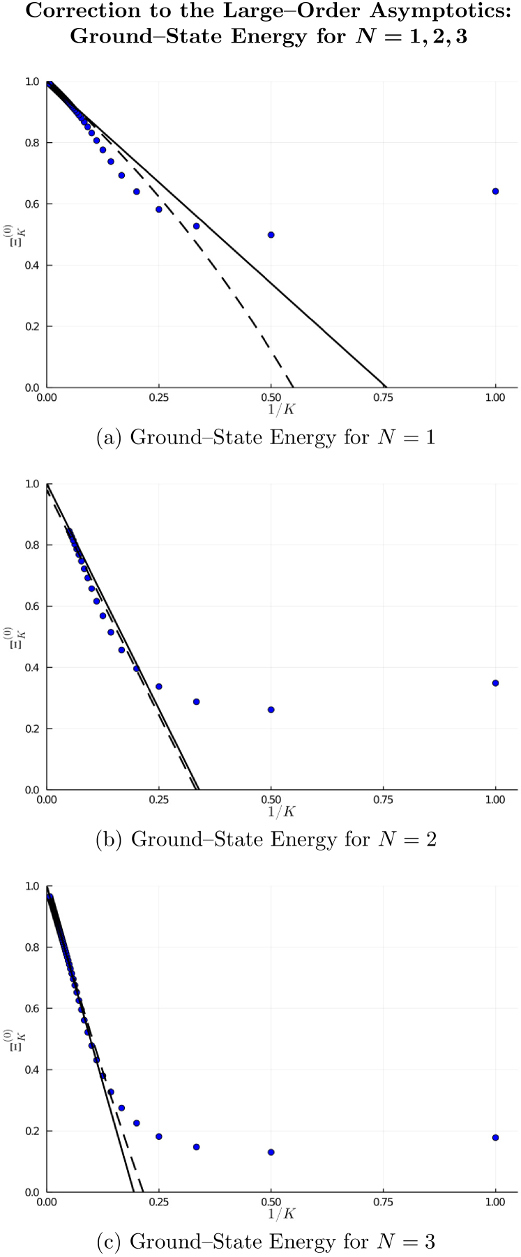
Figure 1: Coefficients of the perturbative expansion of the ground-state of the energy for $N=1,N=2,N=3$ in function of the inverse of the order of perturbation (blue dots). These coefficients have been divided by their leading asymptotic estimate, given in Eq. (87), and have been compared with their subleading order estimate. Dashed black lines include the term $b-1$ term at the denominator of the $1/(K+b-1)$ term in Eq. (89), while solid black lines exclude this term, and follow only the $1/K$ term given in Eq. (88).

III.3 Four-point correlation function

Similarly to the previous subsection, we apply the same ideas to the connected four-point function,

$$C_{i_{1}\,i_{2}\,i_{3}\,i_{4}}(t_{1},t_{2},t_{3},t_{4})=\frac{1}{N(N+2)}\\ \times(\delta_{i_{1}\,i_{2}}\,\delta_{i_{3}\,i_{4}}+\delta_{i_{1}\,i_{3}}\,\delta_{i_{2}\,i_{4}}+\delta_{i_{1}\,i_{4}}\,\delta_{i_{2}\,i_{3}})\\ \times C^{(4)}(t_{2}-t_{1},t_{3}-t_{1},t_{4}-t_{1})\,,$$ (55)

where, according to Eq. (45),

$$C^{(4)}(t_{2},t_{3},t_{4})=\frac{N(N+2)}{3}\,\widetilde{C}^{(4)}(t_{2},t_{3},t_{4})\\ \equiv\frac{N(N+2)}{3}\bigg{[}\langle q_{\hat{\imath}_{1}}(0)q_{\hat{\imath}_{1}}(t_{2})q_{\hat{\imath}_{1}}(t_{3})q_{\hat{\imath}_{1}}(t_{4})\rangle\\ -\widetilde{C}^{(2)}(-t_{2})\widetilde{C}^{(2)}(t_{3}-t_{4})-\widetilde{C}^{(2)}(t_{3}-t_{2})\widetilde{C}^{(2)}(-t_{4})\\ -\widetilde{C}^{(2)}(-t_{3})\widetilde{C}^{(2)}(t_{2}-t_{4})\bigg{]}\,.$$ (56)

In our derivation leading to Eq. (45), we had stressed that the formula is valid for every value that $\hat{\imath}_{1}$ can assume. We now select, for convenience, one particular component with $\hat{\imath}_{1}=1$, which, as we assume, is aligned with the quantization axis for the states in the internal $O(N)$ symmetry group. Hence, we write the relation

$$\langle q_{\hat{\imath}_{1}=1}(0)q_{\hat{\imath}_{1}=1}(t_{2})q_{\hat{\imath}_{1}=1}(t_{3})q_{\hat{\imath}_{1}=1}(t_{4})\rangle\\ =\langle 0|r\cos\theta_{1}{\mathrm{e}}^{-(H-E_{0})\Delta_{3}}\,r\cos\theta_{1}\,{\mathrm{e}}^{-(H-E_{0})\Delta_{2}}\\ r\cos\theta_{1}\,{\mathrm{e}}^{-(H-E_{0})\Delta_{1}}r\cos\theta_{1}|0\rangle+\\ -\widetilde{C}^{(2)}(\Delta_{1})\widetilde{C}^{(2)}(\Delta_{3})-\widetilde{C}^{(2)}(\Delta_{1}+\Delta_{2})\widetilde{C}^{(2)}(\Delta_{2}+\Delta_{3})\\ -\widetilde{C}^{(2)}(\Delta_{1}+\Delta_{2}+\Delta_{3})\widetilde{C}^{(2)}(\Delta_{2}),$$ (57)

where $\Delta_{i}\equiv t_{i+1}-t_{i}$. We then have, with $x_{1}=r\cos\theta_{1}$,

$$\int_{-\infty}^{+\infty}{\mathrm{d}}t_{2}\int_{-\infty}^{+\infty}{\mathrm{d}}t_{3}\int_{-\infty}^{+\infty}{\mathrm{d}}t_{4}\,\widetilde{C}^{(4)}(t_{2},t_{3},t_{4})=\\ =24\sum_{\vec{\eta},\vec{\eta}^{\prime},\vec{\eta^{\prime\prime}}}\frac{\langle 0|x_{1}|\vec{\eta}\rangle\langle\vec{\eta}|x_{1}|\vec{\eta}^{\prime}\rangle\langle\vec{\eta}^{\prime}|x_{1}|\vec{\eta^{\prime\prime}}\rangle\langle\vec{\eta^{\prime\prime}}|x_{1}|0\rangle}{(E_{n}-E_{0})\,(E_{n^{\prime}}-E_{0})\,(E_{n^{\prime\prime}}-E_{0})}\\ -24\sum_{\vec{\eta},\vec{\eta}^{\prime}}\frac{|\langle 0|x_{1}|\vec{\eta}\rangle|^{2}\,|\langle 0|x_{1}|\vec{\eta}^{\prime}\rangle|^{2}(E_{n}+E_{n^{\prime}}-2E_{0})}{2(E_{n^{\prime}}-E_{0})^{2}(E_{n}-E_{0})^{2}}\,.$$ (58)

Using Eq. (93), we have

$$\int_{-\infty}^{+\infty}{\mathrm{d}}t_{2}\int_{-\infty}^{+\infty}{\mathrm{d}}t_{3}\int_{-\infty}^{+\infty}{\mathrm{d}}t_{4}\,\widetilde{C}^{(4)}(t_{2},t_{3},t_{4})\\ =24\sum_{n,\ell,n^{\prime},\ell^{\prime}}\frac{1}{E_{n^{\prime}}-E_{0}}\left[\alpha^{(N)}_{0,\ell}\,\alpha^{(N)}_{\ell,\ell^{\prime}}\frac{S_{00,n\ell}S_{n\ell,n^{\prime}\ell^{\prime}}}{E_{n}-E_{0}}\right]^{2}\\ -24\sum_{n,\ell,n^{\prime},\ell^{\prime}}\frac{\left(\alpha^{(N)}_{0,\ell^{\prime}}\right)^{2}S^{2}_{00,n\ell}\,S^{2}_{00,n^{\prime}\ell^{\prime}}}{(E_{n^{\prime}}-E_{0})^{2}\,(E_{n}-E_{0})}\,.\color[rgb]{0,0,0}$$ (59)

The multiplicities are different if we choose $N=2$ or $N=3$. We can insert them in the definition of the quantity

$$\widetilde{\alpha}^{(N)}_{\ell}=\begin{cases}4\left(\alpha_{0,1}^{(2)}\right)^{4}\delta_{\ell,0}+2\left(\alpha_{0,1}^{(2)}\alpha_{1,2}^{(2)}\right)^{2}\delta_{\ell,2}&\text{for }N=2\,,\\ \left(\alpha_{0,1}^{(3)}\right)^{4}\delta_{\ell,0}+\left(\alpha_{0,1}^{(3)}\alpha_{1,2}^{(3)}\right)^{2}\delta_{\ell,2}&\text{for }N=3\,,\end{cases}$$ (60)

which depend on the factors given in Eqs. (94), (95). Using the angular selection rules, we finally obtain

$$\int_{-\infty}^{+\infty}{\mathrm{d}}t_{2}\int_{-\infty}^{+\infty}{\mathrm{d}}t_{3}\int_{-\infty}^{+\infty}{\mathrm{d}}t_{4}\,\widetilde{C}^{(4)}(t_{2},t_{3},t_{4})\\ =24\sum_{n^{\prime}}\sum_{\ell^{\prime}=0,2}\frac{\widetilde{\alpha}^{(N)}_{\ell^{\prime}}}{E_{n^{\prime}}-E_{0}}\left[\sum_{n}\frac{S_{00,n1}S_{n1,n^{\prime}\ell^{\prime}}}{E_{n}-E_{0}}\right]^{2}\\ -24\,\widetilde{\alpha}^{(N)}_{0}\sum_{n,n^{\prime}}\frac{S^{2}_{00,n1}\,S^{2}_{00,n^{\prime}1}(E_{n}+E_{n^{\prime}}-2E_{0})}{2(E_{n^{\prime}}-E_{0})^{2}(E_{n}-E_{0})^{2}}\\ \sim\frac{3}{N(N+2)}\,\sum_{K}[G^{(4)}(N,1)]_{K}\,g^{K}\,.$$ (61)

Results for low-order perturbative coefficients for the four-point correlation function ($N=2$ and $N=3$) are given in Tables 2 and 3.

III.4 Correlation function with a wigglet insertion

The last quantity we want to look at, within the context of the $O(N)$ theory, is the two-point correlation function with a wigglet insertion,

$$C^{(1,2)}_{i_{1},i_{2}}(t_{2},t_{3})=\frac{\delta_{i_{1}\,i_{2}}}{N}\,C^{(1,2)}(t_{2},t_{3})\,,$$ (62)

where we have defined

$$C^{(1,2)}(t_{2},t_{3})\equiv N\,C^{(1,2)}_{\hat{\imath}_{1}\,\hat{\imath}_{1}}(t_{2},t_{3})=N\,\widetilde{C}^{(1,2)}(t_{2},t_{3})\,.\\$$ (63)

Here, $\widetilde{C}^{(1,2)}(t_{2},t_{3})=C^{(1,2)}_{\hat{\imath}_{1}\,\hat{\imath}_{1}}(t_{2},t_{3})$ is equal to any nonvanishing element within the internal group structure; nonvanishing elements have their first index equal to their second index. One finds

$$\widetilde{C}^{(1,2)}(t_{2},t_{3})=\langle q_{\hat{\imath}_{1}}(0)\,q_{\hat{\imath}_{1}}(t_{2})\,q_{\hat{\imath}_{1}}^{2}(t_{3})\rangle\\ -\langle q_{\hat{\imath}_{1}}(0)\,q_{\hat{\imath}_{1}}(t_{2})\rangle\,\langle q_{\hat{\imath}_{1}}^{2}(t_{3})\rangle\\ -2\langle q_{\hat{\imath}_{1}}(0)\,q_{\hat{\imath}_{1}}(t_{3})\rangle\langle q_{\hat{\imath}_{1}}(t_{2})\,q_{\hat{\imath}_{1}}(t_{3}))\rangle\,.$$ (64)

Setting $\hat{\imath}_{1}=1$ for simplicity and introducing the quantity $x_{1}=r\,\cos\theta_{1}$, for the coordinate along the quantization axis, as before, we can perform the integrals with respect to the time variables, obtaining

$$\int_{-\infty}^{+\infty}{\mathrm{d}}t_{2}\int_{-\infty}^{+\infty}{\mathrm{d}}t_{3}\,\widetilde{C}^{(1,2)}(t_{2},t_{3})\\ =4\sum_{n,\vec{\eta},n^{\prime},\vec{\eta}^{\prime}}\frac{\langle 0|(x_{1})^{2}|n,\vec{\eta}\rangle\langle n,\vec{\eta}|x_{1}|n^{\prime},\vec{\eta}^{\prime}\rangle\langle n^{\prime},\vec{\eta}^{\prime}|x_{1}|n,0\rangle}{(E_{n}-E_{0})\,(E_{n^{\prime}}-E_{0})}\\ +2\sum_{n,\vec{\eta},n^{\prime},\vec{\eta}^{\prime}}\frac{\langle 0|x_{1}|n,\vec{\eta}\rangle\langle n,\vec{\eta}|(x_{1})^{2}|n^{\prime},\vec{\eta}^{\prime}\rangle\langle n^{\prime},\vec{\eta}^{\prime}|x_{1}|0\rangle}{(E_{n}-E_{0})\,(E_{n^{\prime}}-E_{0})}+\\ -2\sum_{n,\vec{\eta}}\frac{|\langle 0|\,x_{1}\,|n,\vec{\eta}\rangle|^{2}\langle 0|\,(x_{1})^{2}\,|0\rangle}{(E_{n}-E_{0})^{2}}-4\left(\sum_{n,\vec{\eta}}\frac{|\langle 0|\,x_{1}\,|n,\vec{\eta}\rangle|^{2}}{(E_{n}-E_{0})}\right)^{2}\\ -8\sum_{n,\vec{\eta},n^{\prime},\vec{\eta}^{\prime}}\frac{|\langle 0|x_{1}|n,\vec{\eta}\rangle|^{2}|\,\langle 0|r\cos\theta_{1}|n^{\prime},\vec{\eta}^{\prime}\rangle|^{2}}{(E_{n^{\prime}}-E_{0})\,(E_{n^{\prime}}+E_{n}-2E_{0})}\,.$$ (65)

Using the radial $S$ matrix elements defined in Eq. (93), and the radial $Q$ matrix elements defined in Eq. (97), we obtain

$$\int_{-\infty}^{+\infty}{\mathrm{d}}t_{2}\int_{-\infty}^{+\infty}{\mathrm{d}}t_{3}\,\widetilde{C}^{(1,2)}(t_{2},t_{3})=\\ 4(2-\delta_{N\,3})\sum_{n,n^{\prime}}\sum_{\ell=0,2}\frac{\beta_{0,\ell}^{(N)}\alpha_{\ell,1}^{(N)}\alpha_{1,0}^{(N)}\,Q_{00,n\ell}S_{n\ell,n^{\prime}1}S_{n^{\prime}1,00}}{(E_{n}-E_{0})(E_{n^{\prime}}-E_{0})}\\ +2(3-2\delta_{N\,3})\sum_{n,n^{\prime}}\frac{\beta_{1,1}^{(N)}\left(\alpha_{1,0}^{(N)}\right)^{2}\,S_{00,n1}Q_{n1,n^{\prime}1}S_{n^{\prime}1,00}}{(E_{n}-E_{0})(E_{n^{\prime}}-E_{0})}\\ -2(2-\delta_{N\,3})\sum_{n}\left(\alpha_{0,1}^{(N)}\right)^{2}\beta_{0,0}^{(N)}\frac{S^{2}_{00,n1}Q_{00,00}}{(E_{n}-E_{0})^{2}}\\ -8(2-\delta_{N\,3})^{2}\sum_{n,n^{\prime}}\frac{\left(\alpha_{0,1}^{(N)}\right)^{2}\,\left(\alpha_{0,1}^{(N)}\right)^{2}\,S^{2}_{00,n1}S^{2}_{00,n^{\prime}1}}{(E_{n^{\prime}}-E_{0})(E_{n^{\prime}}+E_{n}-2E_{0})}\\ -4(2-\delta_{N\,3})^{2}\left[\sum_{n}\left(\alpha_{0,1}^{(N)}\right)^{2}\frac{S_{00,n1}^{2}}{E_{n}-E_{0}}\right]^{2}\,.$$ (66)

We define the angular factors

$$\widetilde{\beta}^{(N)}_{\ell}\equiv \;\begin{cases}2\beta_{0,\ell}^{(2)}\alpha_{\ell,1}^{(2)}\alpha_{1,0}^{(2)}&\qquad(N=2)\,,\\ \beta_{0,\ell}^{(3)}\alpha_{\ell,1}^{(3)}\alpha_{1,0}^{(3)}&\qquad(N=3)\,,\end{cases}$$ (67)

$$\widetilde{\gamma}^{(N)}\equiv \;\begin{cases}3\beta_{1,1}^{(2)}\left(\alpha_{1,0}^{(2)}\right)^{2}&\qquad(N=2)\,,\\ \beta_{1,1}^{(3)}\left(\alpha_{1,0}^{(3)}\right)^{2}&\qquad(N=3)\,.\end{cases}$$ (68)

Using the expressions given in Eqs. (94), (95), (98), and (99) for the angular factors, we finally get

$$\int_{-\infty}^{+\infty}{\mathrm{d}}t_{2}\int_{-\infty}^{+\infty}{\mathrm{d}}t_{3}\,\widetilde{C}^{(1,2)}(t_{2},t_{3})=\\ 4\sum_{n,n^{\prime}}\sum_{\ell=0,2}\widetilde{\beta}^{(N)}_{\ell}\frac{Q_{00,n\ell}S_{n\ell,n^{\prime}1}S_{n^{\prime}1,00}}{(E_{n}-E_{0})(E_{n^{\prime}}-E_{0})}\\ +2\widetilde{\gamma}^{(N)}\sum_{n,n^{\prime}}\frac{S_{00,n1}Q_{n1,n^{\prime}1}S_{n^{\prime}1,00}}{(E_{n}-E_{0})(E_{n^{\prime}}-E_{0})}\\ -2\widetilde{\beta}^{(N)}_{0}\sum_{n}\frac{Q_{00,00}\,S^{2}_{00,n1}}{(E_{n}-E_{0})^{2}}-4\widetilde{\alpha}_{0}^{(N)}\left[\sum_{n}\frac{S_{00,n1}^{2}}{E_{n}-E_{0}}\right]^{2}\\ -8\widetilde{\alpha}_{0}^{(N)}\sum_{n,n^{\prime}}\frac{S^{2}_{00,n1}S^{2}_{00,n^{\prime}1}}{(E_{n^{\prime}}-E_{0})(E_{n^{\prime}}+E_{n}-2E_{0})}\\ \sim\frac{1}{N}\,\sum_{K}[G^{(1,2)}(N,1)]_{K}\,g^{K}\,.$$ (69)

Results for perturbative coefficients $[G^{(1,2)}(N,1)]_{K}$ for the cases $N=2$ and $N=3$, for low orders of perturbation theory, are given in Tables 2 and 3, respectively. This concludes our discussion of the formalism used for obtaining higher orders of perturbation theory for the correlation functions discussed in this articles. We can now proceed to the comparison with the analytic large-order estimates, and the subleading corrections, evaluated in Ref. Giorgini et al. (2020).

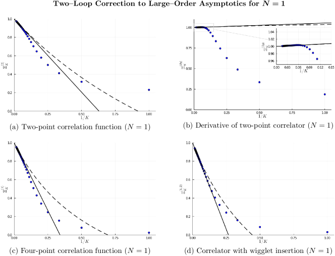
Figure 2: Same as Fig. 1, but the correlation functions in $N=1$.

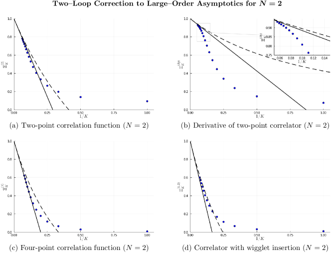
Figure 3: Same as Fig. 2, but for $N=2$.

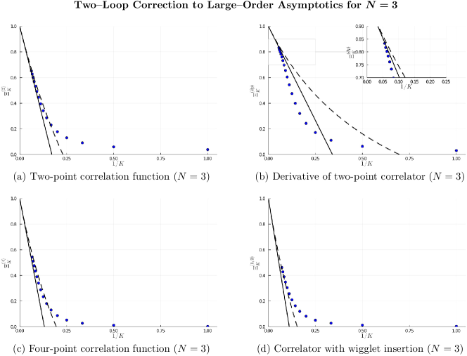
Figure 4: Same as Fig. 2, but for $N=3$.

IV Comparison with Two–Loop Corrections for Large Order

IV.1 Analytic Formulas

In this section, we briefly review the results obtained in Giorgini et al. (2020) concerning the large order behaviour of the ground state energy and of an $M$-point correlation function $G$ for a $D$-dimensional field theory with $N$ components, which can be traced to the two-loop corrections to the instanton configurations that describe the leading factorial growth of the perturbative coefficients.. We refer to the perturbative coefficient of order $K$ as $G_{K}^{(M)}$. When $K$ is large, we can express $G_{K}^{(M)}$ to order $1/K$ as

$$G_{K}^{(M)}=\frac{c(N,D)}{\pi}\,\Gamma\left(K+b\right)\left(\frac{1}{A}\right)^{b}\;\left(-\frac{1}{A}\right)^{K}\;\left[1\right.\\[0.4878pt] \left.-\frac{A\,d(N,D)}{K+b-1}+{\mathcal{O}}(K^{-2})\right]\,,\qquad b=\frac{M+N+D-1}{2}\,,$$ (70)

where $A=4/3$ is the action of the $\phi^{4}$ theory evaluated on the instanton saddle-point multiplied by the coupling constant and with an inverted sign. For large $K$, we can replace $K-1+b\to K$ in the denominator of the second term and identify the $1/K$-correction.

We start with the ground-state energy obtained using the relation in Eq. (49) computing the bracket of the perturbative Hamiltonian with the unperturbed and perturbed ground state eigenfunctions. Specifically, one needs to examine the relation

$$\int_{-\infty}^{+\infty}C^{(0)}(t)\,{\mathrm{d}}t\sim\sum_{K}[G^{(0)}(N,1)]_{K}\,g^{K}\,.$$ (71)

Here, $[G^{(0)}_{N,1}]_{K}$ is the specialization of the general asymptotic perturbative coefficient $G_{K}$ of order $K$ given in Eq. (70) to the ground-state energy function ($M=0$) in one spatial dimension ($D=1$) and for an internal $O(N)$ symmetry group,

$$[G^{(0)}(N,1)]_{K}=\frac{c^{(0)}(N,1)}{\pi}\,\Gamma\left(K+b\right)\left(\frac{1}{A}\right)^{b}\;\left(-\frac{1}{A}\right)^{K}\;\\[0.4878pt] \times\left[1-\frac{A\,d^{(0)}(N,1)}{K+b-1}+{\mathcal{O}}(K^{-2})\right]\,,\qquad b=\frac{N}{2}\,,$$ (72)

where we defined

$$c^{(0)}(N,1)= \;2\pi^{2}\frac{8^{N/2}}{\Gamma(N/2)},$$ (73a)

$$d^{(0)}(N,1)= \;\frac{5}{24}+\frac{5}{2\pi^{2}}-\frac{7\zeta(3)}{4\pi^{2}}$$

$$\;+\left(\frac{9}{16}-\frac{1}{2\pi^{2}}+\frac{7\zeta(3)}{4\pi^{2}}\right)N+\frac{7}{32}\,N^{2}\,.$$ (73b)

For the two point correlation function given in Eq. (49) one needs to examine the relation

$$\int_{-\infty}^{+\infty}C^{(2)}(t)\,{\mathrm{d}}t\sim\sum_{K}[G^{(2)}(N,1)]_{K}\,g^{K}\,.$$ (74)

Here, $[G^{(2)}_{N,1}]_{K}$ is the specialization of the general asymptotic perturbative coefficient $G_{K}$ of order $K$ given in Eq. (70) to the two-point correlation function ($M=2$) in one spatial dimension ($D=1$) and for an internal $O(N)$ symmetry group,

$$[G^{(2)}(N,1)]_{K}=\frac{c^{(2)}(N,1)}{\pi}\,\Gamma\left(K+b\right)\left(\frac{1}{A}\right)^{b}\;\left(-\frac{1}{A}\right)^{K}\;\\[0.4878pt] \times\left[1-\frac{A\,d^{(2)}(N,1)}{K+b-1}+{\mathcal{O}}(K^{-2})\right]\,,\qquad b=1+\frac{N}{2}\,,$$ (75)

where we defined

$$c^{(2)}(N,1)= \;2\pi^{2}\frac{8^{N/2}}{\Gamma(N/2)},$$ (76a)

$$d^{(2)}(N,1)= \;\frac{5}{24}+\frac{5}{2\pi^{2}}-\frac{7\zeta(3)}{4\pi^{2}}$$

$$\;+\left(\frac{9}{16}-\frac{1}{2\pi^{2}}+\frac{7\zeta(3)}{4\pi^{2}}\right)N+\frac{7}{32}\,N^{2}\,.$$ (76b)

For the second derivative of the two-point correlation function at zero momentum, the asymptotic relationship is given in Eqs. (50),

$$\int_{-\infty}^{+\infty}t^{2}\,C^{(2)}(t)\,{\mathrm{d}}t\sim\sum_{K}[G^{(\partial p)}(N,1)]_{K}\,g^{K}\,,$$ (77)

where

$$[G^{(\partial p)}(N,1)]_{K}=\frac{c^{(\partial p)}(N,1)}{\pi}\,\Gamma\left(K+b\right)\left(\frac{1}{A}\right)^{b}\;\\ \times\left(-\frac{1}{A}\right)^{K}\,\left[1-\frac{A\,d^{(\partial p)}(N,1)}{K+b-1}+{\mathcal{O}}(K^{-2})\right]\,,\\ b=1+\frac{N}{2}\,,$$ (78)

with

$$c^{(\partial p)}(N,1)= \;-\pi^{4}\frac{8^{N/2}}{\Gamma(N/2)},$$ (79a)

$$d^{(\partial p)}(N,1)= \;\frac{5}{24}+\frac{4}{\pi^{4}}-\frac{21\,\zeta(3)}{\pi^{4}}-\frac{93\,\zeta(5)}{2\pi^{4}}$$ (79b)

$$\;+\left(-\frac{3}{16}-\frac{6}{\pi^{4}}+\frac{93\zeta(5)}{2\pi^{4}}\right)\,N+\frac{7}{32}\,N^{2}\,.$$

For the four-point correlation function, the relationship is, from Eqs. (61),

$$\int_{-\infty}^{+\infty}{\mathrm{d}}t_{2}\int_{-\infty}^{+\infty}{\mathrm{d}}t_{3}\int_{-\infty}^{+\infty}{\mathrm{d}}t_{4}\,C^{(4)}(t_{2},t_{3},t_{4})\\ \sim\sum_{K}[G^{(4)}(N,1)]_{K}\,g^{K}\,,$$ (80)

where

$$[G^{(4)}(N,1)]_{K}=\frac{c^{(4)}(N,1)}{\pi}\,\Gamma\left(K+b\right)\left(\frac{1}{A}\right)^{b}\;\left(-\frac{1}{A}\right)^{K}\;\\[0.4878pt] \times\left[1-\frac{A\,d^{(4)}(N,1)}{K+b-1}+{\mathcal{O}}(K^{-2})\right]\,,\qquad b=2+\frac{N}{2}\,,$$ (81)

with

$$c^{(4)}(N,1)= \;4\pi^{4}\frac{8^{N/2}}{\Gamma(N/2)},$$ (82a)

$$d^{(4)}(N,1)= \;\frac{5}{24}+\frac{13}{\pi^{2}}-\frac{7\,\zeta(3)}{2\pi^{2}}$$ (82b)

$$\;+\left(\frac{9}{16}-\frac{1}{\pi^{2}}+\frac{7\zeta(3)}{2\pi^{2}}\right)\,N+\frac{7}{32}\,N^{2}\,.$$

For the two-point correlation function with a wigglet insertion, the relationship is, from Eqs. (69),

$$\int_{-\infty}^{+\infty}{\mathrm{d}}t_{2}\int_{-\infty}^{+\infty}{\mathrm{d}}t_{3}\,C^{(1,2)}(t_{2},t_{3})\\ \sim\sum_{K}[G^{(1,2)}(N,1)]_{K}\,g^{K}\,,$$ (83)

where

$$G^{(1,2)}_{K}=\frac{c^{(1,2)}(N,1)}{\pi}\,\Gamma\left(K+b\right)\left(\frac{1}{A}\right)^{b}\;\left(-\frac{1}{A}\right)^{K}\;\\[0.4878pt] \times\left[1-\frac{A\,d^{(1,2)}(N,1)}{K+b-1}+{\mathcal{O}}(K^{-2})\right]\,,\qquad b=2+\frac{N}{2}\,,$$ (84)

with

$$c^{(1,2)}(N,1)= \;8\pi^{2}\frac{8^{N/2}}{\Gamma(N/2)},$$ (85a)

$$d^{(1,2)}(N,1)= \;\frac{35}{24}+\frac{5}{2\pi^{2}}-\frac{7\,\zeta(3)}{4\pi^{2}}$$ (85b)

$$\;+\left(\frac{15}{16}-\frac{1}{2\pi^{2}}+\frac{7\zeta(3)}{4\pi^{2}}\right)\,N+\frac{7}{32}\,N^{2}\,.$$

For reference, the first few perturbative coefficients $[G^{(2)}(N,1)]_{K}$, $[G^{(\partial p)}(N,1)]_{K}$, $[G^{(4)}(N,1)]_{K}$, and $[G^{(1,2)}(N,1)]_{K}$, for $K=0,1,2,3,4,5$ and $10$, for the internal $O(N)$ symmetry group, with $N=1,2,3$, are also given in Tables 1—3.

IV.2 Significance of the Two–Loop Correction

In Figs. 1—4, we plot the asymptotic expression of the coefficients of the perturbative expansion of the ground-state energy and of the correlation functions as a function of the inverse of the order of perturbation $K$. These coefficients have been divided by their leading order expression reported in Eq. (70), that is the expression proportional to

$$[Q^{(M)}]_{K}=\frac{c(N,1)}{\pi}\,\Gamma\left(K+b\right)\left(\frac{1}{A}\right)^{(M+N)/2}\;\left(-\frac{1}{A}\right)^{K}\,.$$ (86)

and they read

$$[\Xi^{(M)}]_{K}=\frac{[G^{(M)}]_{K}}{[Q^{(M)}]_{K}}.$$ (87)

These coefficients have been compared with their next-to-leading order estimate, i.e., with the multiplicative term

$$[\Xi^{(M)}]_{K}\approx\mu_{K}^{(M)}=1-A\frac{d(M,N)}{K}\,,$$ (88)

and with

$$[\Xi^{(M)}]_{K}\approx\nu_{K}^{(M)}=1-A\frac{d(M,N)}{K+b-1}\\ =1-A\frac{d(M,N)}{K}+A\frac{(b-1)d(M,N)}{K^{2}}+O\left(\frac{1}{K}\right)^{3}\,,$$ (89)

which carries a (part of the) next-to-next-to-leading $1/K^{2}$ correction term.

In Figs. 1–4, we observe a good agreement between the asymptotic estimate of the perturbative coefficients of the correlation functions obtained in Ref. Giorgini et al. (2020) with the explicit higher-order calculations reported here. Indeed, the improvement of the agreement upon the inclusion of the next-to-leading order correction is quite remarkable. The calculation of the large-order behavior of the perturbative expansion of the correlation functions for $N>1$ was much more computationally expensive with respect to the case $N=1$, therefore it was possible to obtain less orders of perturbation.

V Conclusions

In this article, we have discussed the explicit higher-order calculation of the perturbative expansions of correlation functions for the $O(N)$ quartic anharmonic oscillator. We discussed the $N=1$ quantum anharmonic oscillator in Sec. II. In Sec. III, we discussed the formulation of the perturbative expansion of the correlation functions of the $O(N)$ quantum anharmonic oscillator, where the internal symmetry group is assumed to be $O(2)$ or $O(3)$, and general formulas are given which allow us to enter a unified evaluation of the perturbative expansions. Specifically, we considered the two-point correlation function in Sec. III.2, the four-point correlator in Sec. III.3, and the correlation function with a wigglet insertion in Sec. III.4. The comparison with analytic results together with a review of the previously (Ref. Giorgini et al. (2020)) obtained results for the large-order behavior of the correlation functions was carried out in Sec. IV. The data in Figs. 1—3 underline the importance of the next-to-leading order correction to the large-order factorial growth of the perturbative coefficients for the demonstration of the agreement of asymptotic estimates and explicit perturbative calculations.

Let us take, as an example, the coefficient of order $g^{8}$ (the “eight-loop coefficient”) for the two-point correlation function in the $O(3)$ model. The explicit result is

$$[G^{(4)}_{N=3}]_{K=8}\simeq 3.03\cdot 10^{6}\,.$$ (90)

The leading asymptotic term is

$$[G^{(4)}_{N=3,1}]_{K=8}\approx 8.87\cdot 10^{6}\,.$$ (91)

With the inclusion of the two-loop (order $1/K$) correction, we find the (much better) estimate

$$[G^{(4)}_{N=3,1}]_{K=8}\approx 2.38\cdot 10^{6}\,.$$ (92)

which differs from the the exact perturbative coefficient by roughly $20$ percent. At order $K=10$, we already observe $93$ percent agreement, whereas at order $K=14$, the agreement it is slightly better than $97$ percent. In some other cases, the agreement is surprisingly good even at very low orders. For example, for $N=2$, the two-loop large-order estimate of the coefficient of the four-point correlation function agree with the exact perturbative coefficient at the level of 98 percent, in eight-loop order ($K=8$).

The tests presented here are essential to have a good starting point from which to extend the calculations to field theory, i.e., to the case $D>1$, where this type of checks are not possible anymore. Specifically, the agreement between these two different approaches ensures the correctness of the method described in Giorgini et al. (2020), which can be then generalized to obtain the perturbative expression of the correlation functions for two and three dimensional $N$-vector model where is not possible to use the conventional techniques of perturbation theory. We recall that, irrespective of the dimension $D$, the same dispersion relation relates the large-order growth of the coefficients of a correlation function with the behaviour at small orders of perturbation of its imaginary part for negative coupling.

Appendix A Some useful definitions and identities

A.1 Matrix elements

In this section, we will derive the expression for the various angular matrix elements denoted as $\alpha$, and $\beta$, which appear in the main text. We start considering the matrix element $\langle n,\vec{\eta}|r\cos\theta_{1}|n^{\prime},\vec{\eta}^{\prime}\rangle$. If the coordinate $r\cos\theta_{1}$ is aligned with the quantization axis, then the only nonvanishing transition matrix element will be obtained for all magnetic projections equal to zero. We can therfore assume that $\ket{n,\vec{\eta}}\equiv\ket{n,\ell,0,\dots,0}$ and $\ket{n^{\prime},\vec{\eta}^{\prime}}\equiv\ket{n^{\prime},\ell^{\prime},0,\dots,0}$. Under these assumptions, we can write the matrix element as

$$\langle n,\vec{\eta}|r\cos\theta_{1}|n^{\prime},\vec{\eta}^{\prime}\rangle=S_{n\ell,n^{\prime}\ell^{\prime}}\,\alpha^{(N)}_{\ell,\ell^{\prime}}$$ (93a)

where the radial part is given as follows,

$$S_{n\ell,n^{\prime}\ell^{\prime}} \equiv\int dr\,r^{N}R_{n\ell}(r)R_{n^{\prime}\ell^{\prime}}(r)$$ (93b)

$$\alpha^{(N)}_{\ell,\ell^{\prime}} \equiv\int{\mathrm{d}}\theta_{1}\dots\mathrm{d}\theta_{N-1}\,\cos(\theta_{1})J(\theta_{1},\dots,\theta_{N-1})$$

$$\;\times Y^{0\dots 0*}_{\ell}(\theta_{1},\dots,\theta_{N-1})\,Y^{0\dots 0}_{\ell^{\prime}}(\theta_{1},\dots,\theta_{N-1})\,,$$ (93c)

and $J(\theta_{1},\dots,\theta_{N-1})$ is the Jacobian due to the hyperspherical change of coordinates.

Due to the orthogonality relations between the hyperspherical harmonics, only few of the $\alpha^{(N)}_{\ell,\ell^{\prime}}$ terms are non-zero. For example, if $\ell=0$, then we have for $N=2$ and $N=3$ respectively,

$$\alpha^{(2)}_{0,\ell^{\prime}} =\frac{1}{2}\left(\delta_{\ell^{\prime},1}+\delta_{\ell^{\prime},-1}\right)\,,$$ (94a)

$$\alpha^{(3)}_{0,\ell^{\prime}} =\frac{1}{\sqrt{3}}\delta_{\ell^{\prime},1}\,.$$ (94b)

When $\ell=1$, one instead obtains

$$\alpha^{(2)}_{1,\ell^{\prime}} =\frac{1}{2}\left(\delta_{\ell^{\prime},0}+\delta_{\ell^{\prime},2}\right)\,,$$ (95a)

$$\alpha^{(3)}_{1,\ell^{\prime}} =\frac{1}{\sqrt{3}}\delta_{\ell^{\prime},0}+\frac{2}{\sqrt{15}}\delta_{\ell^{\prime},2}\,.$$ (95b)

In general, one has

$$\alpha_{\ell,\ell^{\prime}}^{(2)}=\frac{1}{2}\left(\delta_{\ell^{\prime},\ell+1}+\delta_{\ell^{\prime},\ell-1}\right).$$ (96)

For the two-point function with a wigglet insertion, we also have to consider the matrix element $\langle n,\vec{\eta}|(r\cos\theta_{1})^{2}|n^{\prime},\vec{\eta}^{\prime}\rangle$ where $\ket{n,\vec{\eta}}\equiv\ket{n,\ell,0,\dots,0}$ and $\ket{n^{\prime},\vec{\eta}^{\prime}}\equiv\ket{n^{\prime},\ell^{\prime},0,\dots,0}$. It can be written as

$$\langle n,\vec{\eta}|(r\cos\theta_{1})^{2}|n^{\prime},\vec{\eta}^{\prime}\rangle=Q_{n\ell,n^{\prime}\ell^{\prime}}\,\beta^{(N)}_{\ell,\ell^{\prime}}\,,$$ (97a)

where

$$Q_{n\ell,n^{\prime}\ell^{\prime}}\equiv \;\int{\mathrm{d}}r\,r^{N+1}\,R_{n\ell}(r)\,R_{n^{\prime}\ell^{\prime}}(r)\,,$$ (97b)

$$\beta^{(N)}_{\ell,\ell^{\prime}}\equiv \;\int{\mathrm{d}}\theta_{1}\dots\mathrm{d}\theta_{N-1}\,(\cos(\theta_{1}))^{2}J(\theta_{1},\dots,\theta_{N-1})$$

$$\;\times Y^{0\dots 0*}_{\ell}(\theta_{1},\dots,\theta_{N-1})\;Y^{0\dots 0}_{\ell^{\prime}}(\theta_{1},\dots,\theta_{N-1})\,.$$ (97c)

Also in this case, because of the orthogonality relations between the hyperspherical harmonics, only few of the $\beta^{(N)}_{\ell,\ell^{\prime}}$ terms are non-zero. For example, if $\ell=0$, then we have for $N=2$ and $N=3$, respectively

$$\beta^{(2)}_{0,\ell^{\prime}} =\frac{1}{4}\left(2\delta_{\ell^{\prime},0}+\delta_{\ell^{\prime},2}+\delta_{\ell^{\prime},-2}\right)\,,$$ (98a)

$$\beta^{(3)}_{0,\ell^{\prime}} =\frac{1}{3}\left(\delta_{\ell^{\prime},0}+\frac{2}{\sqrt{5}}\delta_{\ell^{\prime},2}\right)\,.$$ (98b)

When $\ell=1$, instead, one has

$$\beta^{(2)}_{1,\ell^{\prime}}= \;\frac{1}{4}\left(\delta_{\ell^{\prime},-1}+2\delta_{\ell^{\prime},1}+\delta_{\ell^{\prime},3}\right)\,,$$ (99a)

$$\beta^{(2)}_{-1,\ell^{\prime}}= \;\frac{1}{4}\left(2\delta_{\ell^{\prime},-1}+\delta_{\ell^{\prime},1}+\delta_{\ell^{\prime},-3}\right)\,$$ (99b)

$$\beta^{(3)}_{1,\ell^{\prime}}= \;\frac{1}{5}\left(3\,\delta_{\ell^{\prime},1}+2\sqrt{\frac{3}{7}}\,\delta_{\ell^{\prime},3}\right)\,.$$ (99c)

The above formulas can be used to perform all required angular integrals for the correlation functions considered in our investigations.

A.2 Case $\maybebm{N=3}$

For $N=3$, the coefficients $\alpha_{\ell,\ell^{\prime}}^{(N=3)}$ and $\beta_{\ell,\ell^{\prime}}^{(N=3)}$ can be written in terms of the Gaunt coefficients $Y^{\ell\ell^{\prime}\ell^{\prime\prime}}_{mm^{\prime}m^{\prime\prime}}$ defined as the integral over three spherical harmonics

$$\begin{split}Y^{\ell\ell^{\prime}\ell^{\prime\prime}}_{mm^{\prime}m^{\prime\prime}}&=\int_{0}^{2\pi}{\mathrm{d}}\varphi\,\int_{0}^{\pi}{\mathrm{d}}\theta\sin(\theta)\\ &\;\times Y^{*}_{\ell\,m}(\theta,\varphi)\,Y_{\ell^{\prime}m^{\prime}}(\theta,\varphi)\,Y_{\ell^{\prime\prime}m^{\prime\prime}}(\theta,\varphi)\,.\end{split}$$ (100)

By writing $\cos(\theta)$ and $\cos(\theta)^{2}$ in terms of spherical harmonics we get

$$\alpha^{(3)}_{\ell,\ell^{\prime}}\equiv 2\sqrt{\frac{\pi}{3}}Y^{\ell 1\ell^{\prime}}_{000}\,,$$ (101)

and

$$\beta^{(3)}_{\ell,\ell^{\prime}}\equiv\frac{1}{3}\left(4\sqrt{\frac{\pi}{5}}\,Y^{\ell 2\ell^{\prime}}_{000}+2\sqrt{2}\,Y^{\ell 0\ell^{\prime}}_{000}\right)\,.$$ (102)

Alternatively, the integral appearing in Eq. (100) can be interpreted using the Wigner-Eckart theorem and can be written as the product of the Clebsch-Gordan coefficient corresponding to the quantum numbers $\ell$, $\ell^{\prime}$, $\ell^{\prime\prime}$, $m$, $m^{\prime}$, and $m^{\prime\prime}$, and the reduced matrix element of the spherical harmonic tensor $Y^{m^{\prime}}_{\ell^{\prime}}$, as

$$\int_{0}^{2\pi}{\mathrm{d}}\varphi\int_{0}^{\pi}{\mathrm{d}}\theta\sin(\theta)\,Y^{*}_{\ell\,m}(\theta,\varphi)\,Y_{\ell^{\prime}\,m^{\prime}}(\theta,\varphi)\,Y_{\ell^{\prime\prime}\,m^{\prime\prime}}(\theta,\varphi)\\ =(-1)^{\ell^{\prime}-\ell^{\prime\prime}+\ell}\frac{C_{\ell^{\prime}m^{\prime}\ell^{\prime\prime}m^{\prime\prime}}^{\ell m}}{\sqrt{2\ell+1}}\langle\ell||\vec{Y}_{\ell^{\prime}}||\ell^{\prime\prime}\rangle,$$ (103)

where the reduced matrix can be expressed using a $3j$ symbol with three zero magnetic projections

$$\langle\ell||\vec{Y}_{\ell^{\prime}}||\ell^{\prime\prime}\rangle=(-1)^{\ell}\sqrt{\frac{(2\ell+1)(2\ell^{\prime}+1)(2\ell^{\prime\prime}+1)}{4\pi}}\\ \times\left(\begin{matrix}\ell&\ell^{\prime}&\ell^{\prime\prime}\\ 0&0&0\end{matrix}\right).$$ (104)

Using this convention the coefficients $\alpha_{\ell,\ell^{\prime}}^{(3)}$ and $\beta_{\ell,\ell^{\prime}}^{(3)}$ will read

$$\alpha^{(3)}_{\ell,\ell^{\prime}}\equiv(-1)^{1-\ell^{\prime}+\ell}\,2\sqrt{\frac{\pi}{3}}\,\frac{C_{10\ell^{\prime}m^{\prime}}^{\ell m}}{\sqrt{2\ell+1}}\,\langle\ell||\vec{Y}_{1}||\ell^{\prime}\rangle\,,$$ (105)

and

$$\beta^{(3)}_{\ell,\ell^{\prime}}\equiv\frac{1}{3}\,\bigg{(}(-1)^{2-\ell^{\prime}+\ell}4\sqrt{\frac{\pi}{5}}\,\frac{C_{20\ell^{\prime}m^{\prime}}^{\ell m}}{\sqrt{2\ell+1}}\,\langle\ell||\vec{Y}_{2}||\ell^{\prime}\rangle\\ +(-1)^{-\ell^{\prime}+\ell}2\sqrt{2}\frac{C_{00\ell^{\prime}m^{\prime}}^{\ell m}}{\sqrt{2\ell+1}}\,\langle\ell||\vec{Y}_{0}||\ell^{\prime}\rangle\bigg{)}\,.$$ (106)

These results are in agreement with the formulas obtained in Appendix A.1.

Appendix B Alternative Procedure

The perturbative treatment of the radial part can be accomplished by a direct mapping of the procedure outlined in Eqs. (2)—(8) onto a computer algebra system. However, it is useful to delineate an alternative procedure to compute the eigenvalues and eigenfunctions of the perturbed three dimensional harmonic oscillator. We will deal with the $N=3$ case; the generalization to $N=2$ is relatively straightforward. We adapt to our case the results of Ref. Ehlenberger and Mendelsohn (1972), where the computation has been carried out for a general central field perturbation. The eigenvalues and eigenfunctions of our Schrödinger equation

$$\left(-\vec{\nabla}^{2}+r^{2}+\frac{g}{2}r^{4}\right)\Psi_{n\ell m}(r,\theta,\varphi)\\ =\alpha_{n\ell}\Psi_{n\ell m}(r,\theta,\varphi)\,,\qquad\alpha_{n\ell}=2E_{n\ell}\,,$$ (107)

where $E_{n\ell}$ can be written as a perturbative series in the coupling parameter $g$,

$$\alpha_{n\ell}= \;\sum_{K=0}^{\infty}\alpha_{n\ell,K}\,g^{K}\,,$$ (108a)

$$\Psi_{n\ell m}(r,\theta,\varphi)= \;R_{n\ell}(r)\,Y_{\ell\,m}(\theta,\varphi)\,,$$ (108b)

$$R_{n\ell}(r)= \;{\mathcal{N}}_{n\ell}\,{\mathrm{e}}^{-r^{2}/2}\,r^{\ell}\,\sum_{K=0}^{\infty}u_{n\ell}^{(K)}(r^{2})\,g^{K}\,,$$ (108c)

where ${\mathcal{N}}_{n\ell}={\mathcal{N}}_{n\ell}^{(N=3)}$ is defined in Eq. (31). Each coefficient $u_{n\ell}^{i}(r^{2})$ can be expressed as a linear combination of the eigenfunctions of the unperturbed case (it can be shown that only $4K$ terms will contribute to the $K$th order perturbation)

$$u_{n\ell}^{(K)}(r^{2})= \;\sum_{j=\max(q_{n\ell}-2K,0)}^{q_{n\ell}+2K}A_{Kj}\,L_{j}^{\ell+\frac{1}{2}}(r^{2})$$ (109a)

$$q_{n\ell}= \;\alpha_{n\ell,0}-3-2\ell=\frac{1}{2}(n-\ell).$$ (109b)

The coefficients $\alpha_{n\ell,K}$ and $A_{Kj}$ can be determined from Eqs. (32) and (33) of Ref. Ehlenberger and Mendelsohn (1972) by setting $B_{j}=\frac{\delta_{1j}}{2}$. Special cases are

$$A_{0,j}=\delta_{j,q_{n\ell}},\quad A_{K,q_{n\ell}}=0\;\forall K>0\,.$$ (110)

However, there are some typos in the passages of the paper and we report here a corrected version of the main passages needed to arrive to the result. We use the following recursive relation of the generalized Laguerre polynomials,

$$r^{m}L^{\ell+\frac{1}{2}}_{j}(r^{2})=\sum_{n=0}^{2m}a(m,n,j)\,L^{\ell+\frac{1}{2}}_{j+m-n}(r^{2})\,,$$ (111)

where

$$a(m,n,j)=\frac{(-1)^{m-n}(m!)^{2}}{\Gamma(j+m-n+\ell+\frac{3}{2})}\\ \times\sum_{k=\max(0,j-n)}^{\min(j+m-n,j)}\frac{\binom{j+m-n}{k}\,\Gamma(m+k+\ell+\frac{3}{2})}{(j-k)!(n-j+k)!(m-j+k)!}.$$ (112)

We can then rewrite Eq. (26) of Ehlenberger and Mendelsohn (1972) as

$$\sum_{j=0}^{\infty}(q_{n\ell}-j)A_{Kj}\,L_{j}^{\ell+\frac{1}{2}}(r^{2})\\ =\frac{1}{8}\sum_{w=0}^{K-1}\delta_{1(K-w)}\sum_{j=0}^{\infty}A_{wj}\sum_{i=0}^{2(K-w+1)}a(K-w+1,i,j)\,\\ \times L_{j+K-w+1-i}^{\ell+\frac{1}{2}}(r^{2})-\frac{1}{4}\sum_{w=0}^{K-1}\alpha_{n\ell}^{(K-w)}\sum_{j=0}^{\infty}A_{wj}L_{j}^{\ell+\frac{1}{2}}(r^{2})\\ =\frac{1}{8}\sum_{j=0}^{\infty}A_{(K-1)j}\sum_{i=j-2}^{j+2}a(2,j+2-i,j)\,L_{i}^{\ell+\frac{1}{2}}(r^{2})\\ -\frac{1}{4}\sum_{w=0}^{K-1}\alpha_{n\ell}^{(K-w)}\sum_{j=0}^{\infty}A_{wj}L_{j}^{\ell+\frac{1}{2}}(r^{2})\,.$$ (113)

For a specific value of $L_{s}^{\ell+\frac{1}{2}}(r^{2})$, with the convention

$$\Theta(0)=1$$ (114)

for the Heaviside step function $\Theta$, we get

$$A_{Ks}=\frac{1}{8(q_{n\ell}-s)}\sum_{j=0}^{\infty}A_{(K-1)j}\,a(2,j+2-s,j)\\ \times\Theta(2-|s-j|)-\frac{1}{4(q_{n\ell}-s)}\sum_{w=0}^{K-1}\alpha_{n\ell}^{(K-w)}A_{w,s}\\ =\frac{1}{8(q_{n\ell}-s)}\sum_{\max(j=q_{n\ell}-2(K-1),0)}^{q_{n\ell}+2(K-1)}A_{(K-1)j}\,a(2,j+2-s,j)\\ -\frac{1}{4(q_{n\ell}-s)}\sum_{w=0}^{K-1}\alpha_{n\ell}^{(K-w)}A_{w,s}\,\alpha_{n\ell,K}\\ =\frac{1}{2}\sum_{j=\max(q_{n\ell}-2(K-1),0)}^{q_{n\ell}+2(K-1)}\,A_{(K-1)j}a(2,j+2-q_{n\ell},j)\,.$$ (115)

We can therefore write a recursive relation that will provide an expression for the perturbative coefficients of the eigenvalues and eigenfunctions of the Schrödinger equation. The two-dimensional case can be derived from three-dimensional one using the expression for the eigenfunctions reported in Eq. (29).

References

- (1) See the URL https://researchoutreach.org/articles/dealing-diminishing-returns-quantum-perturbations/.
- Brézin et al. (1977a) E. Brézin, G. Parisi, and J. Zinn-Justin, “Perturbation theory at large orders for a potential with degenerate minima,” Phys. Rev. D 16, 408–412 (1977a).
- Brézin and Parisi (1978) E. Brézin and G. Parisi, “Critical exponents and large-order behavior of perturbation theory,” J. Stat. Phys. 19, 269 (1978).
- Dyson (1952) F. J. Dyson, “Divergence of Perturbation Theory in Quantum Electrodynamics,” Phys. Rev. 85, 631–632 (1952).
- Jentschura and Zinn-Justin (2004) U. D. Jentschura and J. Zinn-Justin, “Instanton Effects in Quantum Mechanics and Resurgent Expansions,” Phys. Lett. B 596, 138–144 (2004).
- Zinn-Justin and Jentschura (2004a) J. Zinn-Justin and U. D. Jentschura, “Multi-instantons and exact results I: Conjectures, WKB expansions, and instanton interactions,” Ann. Phys. (N.Y.) 313, 197–267 (2004a).
- Zinn-Justin and Jentschura (2004b) J. Zinn-Justin and U. D. Jentschura, “Multi-instantons and exact results II: Specific cases, higher-order effects, and numerical calculations,” Ann. Phys. (N.Y.) 313, 269–325 (2004b).
- Bender and Wu (1969) C. M. Bender and T. T. Wu, “Anharmonic oscillator,” Phys. Rev. 184, 1231–1260 (1969).
- Bender and Wu (1971) C. M. Bender and T. T. Wu, “Large–Order Behavior of Perturbation Theory,” Phys. Rev. Lett. 27, 461–465 (1971).
- Bender and Wu (1973) C. M. Bender and T. T. Wu, “Anharmonic oscillator. II. A Study of Perturbation Theory in Large Order,” Phys. Rev. D 7, 1620–1636 (1973).
- Brézin et al. (1977b) E. Brézin, J. C. LeGuillou, and J. Zinn-Justin, “Perturbation theory at large order. I. The interaction,” Phys. Rev. D 15, 1544–1557 (1977b).
- Brézin et al. (1977c) E. Brézin, J. C. LeGuillou, and J. Zinn-Justin, “Perturbation theory at large order. II. Role of the vacuum instability,” Phys. Rev. D 15, 1558–1564 (1977c).
- Jentschura and Zinn-Justin (2011) U. D. Jentschura and J. Zinn-Justin, “Multi-instantons and exact results IV: Path integral formalism,” Ann. Phys. (N.Y.) 326, 2186–2242 (2011).
- Malatesta et al. (2017) E. M. Malatesta, G. Parisi, and T. Rizzo, “Two-loop corrections to large order behavior of theory,” Nucl. Phys. B 922, 293–318 (2017).
- Giorgini et al. (2020) L. T. Giorgini, U. D. Jentschura, E. M. Malatesta, T. Rizzo, G. Parisi, and J. Zinn-Justin, “Two–Loop Corrections to the Large–Order Behavior of Correlation Functions in the One–Dimensional –Vector Model,” Phys. Rev. D 101, 125001 (2020).
- Zinn-Justin (2005) J. Zinn-Justin, Path Integrals in Quantum Mechanics (Oxford University Press, Oxford, 2005) [French version: Intégrale de Chemin en Mécanique Quantique: Introduction, CNRS Éditions, Les Ulis, 2002].
- Jentschura and Sapirstein (2018) U. D. Jentschura and J. Sapirstein, “Green function of the Poisson equation: ,” J. Phys. Commun. 2, 015026 (2018).
- Karimi et al. (2004) E. Karimi, R. W. Boyd, P. de la Hoz, H. de Guise, J. Řeháček, Z. Hradil, A. Aiello, G. Leuchs, and L. L. L. L. Sánchez-Soto, “Radial quantum number of Laguerre-Gauss modes,” Phys. Rev. A 89, 063813 (2004).
- Varshalovich et al. (1988) D. A. Varshalovich, A. N. Moskalev, and V. K. Khersonskii, Quantum Theory of Angular Momentum (World Scientific, Singapore, 1988).
- Abramowitz and Stegun (1972) M. Abramowitz and I. A. Stegun, Handbook of Mathematical Functions, 10th ed. (National Bureau of Standards, Washington, D. C., 1972).
- Zinn-Justin (2021) J. Zinn-Justin, Quantum Field Theory and Critical Phenomena, 5th ed. (Oxford University Press, Oxford, 2021).
- Bethe and Salpeter (1957) H. A. Bethe and E. E. Salpeter, Quantum Mechanics of One- and Two-Electron Atoms (Springer, Berlin, 1957).
- Zinn-Justin (1981) J. Zinn-Justin, “Expansion around instantons in quantum mechanics,” J. Math. Phys. 22, 511–520 (1981).
- Zinn-Justin (1984) J. Zinn-Justin, J. Math. Phys. 25, 549–555 (1984).
- Ehlenberger and Mendelsohn (1972) A. G. Ehlenberger and L. B. Mendelsohn, “High Order Perturbation Theory for a Generalized Central Field Perturbation of the Three-Dimensional Harmonic Oscillator,” J. Chem. Phys. 56, 586–591 (1972).