2021
[1,2]\fnmJason D. \surMcEwen
1]\orgdivMullard Space Science Laboratory (MSSL), \orgnameUniversity College London (UCL), \orgaddress\cityDorking, \postcodeRH5 6NT, \countryUK
2]\orgnameAlan Turing Institute, \orgaddress\cityLondon, \postcodeNW1 2DB, \countryUK
Machine learning assisted Bayesian model comparison: learnt harmonic mean estimator
Abstract
We resurrect the infamous harmonic mean estimator for computing the marginal likelihood (Bayesian evidence) and solve its problematic large variance. The marginal likelihood is a key component of Bayesian model selection to evaluate model posterior probabilities; however, its computation is challenging. The original harmonic mean estimator, first proposed by Newton and Raftery in 1994, involves computing the harmonic mean of the likelihood given samples from the posterior. It was immediately realised that the original estimator can fail catastrophically since its variance can become very large (possibly not finite). A number of variants of the harmonic mean estimator have been proposed to address this issue although none have proven fully satisfactory. We present the learnt harmonic mean estimator, a variant of the original estimator that solves its large variance problem. This is achieved by interpreting the harmonic mean estimator as importance sampling and introducing a new target distribution. The new target distribution is learned to approximate the optimal but inaccessible target, while minimising the variance of the resulting estimator. Since the estimator requires samples of the posterior only, it is agnostic to the sampling strategy used. We validate the estimator on a variety of numerical experiments, including a number of pathological examples where the original harmonic mean estimator fails catastrophically. We also consider a cosmological application, where our approach leads to 3 to 6 times more samples than current state-of-the-art techniques in 1/3 of the time. In all cases our learnt harmonic mean estimator is shown to be highly accurate. The estimator is computationally scalable and can be applied to problems of dimension and beyond. Code implementing the learnt harmonic mean estimator is made publicly available.
keywords:
model selection, Bayesian statistics, marginal likelihood, Bayesian evidence, machine learning1 Introduction
Model selection is a critical task in order to ascertain an appropriate statistical model to describe observational data. In the Bayesian formalism, model selection requires computing the marginal likelihood, the average likelihood of a model over its prior probability space, given observational data. The marginal likelihood (also called the Bayesian evidence) may then be used to compute model posterior odds and assign relative probabilities to different models. Computing the marginal likelihood is therefore a key ingredient in Bayesian inference. However, computing the marginal likelihood in practice requires the evaluation of a high-dimensional integral, which is computationally challenging.
The Bayesian formalism is one of the most common approaches to statistical inference. Consider the estimation of unknown parameters (typically ) from observed data (typically ), under a statistical model relating the data to the parameters. Given the data and model , inferences of the parameters are based on their posterior distribution through Bayes’ theorem by
| (1) |
where for model the likelihood specifies the probability of the data given the parameters and encodes prior information about the parameters. The denominator , termed the marginal likelihood or Bayesian evidence, measures the probability of the observed data under model . For notational brevity we denote the likelihood by , the prior by and the marginal likelihood by . We drop the explicit dependence on the model , except where explicitly required. For parameter inference the marginal likelihood can be ignored (since it simply normalises the posterior) and the shape of the posterior can be explored using Markov chain Monte Carlo (MCMC) sampling techniques, e.g. Metropolis-Hastings sampling (Metropolis et al, 1953; Hastings, 1970).
For Bayesian model selection it is necessary to compute the marginal likelihood given by
| (2) |
The marginal likelihood is of critical importance for Bayesian model selection since it is required to compute the posterior probabilities of models. Noting Bayes’ theorem, the relative posterior probability of competing models and is given by
| (3) |
In the absence of prior information regarding model preferences it is reasonable to take the ratio of model prior probabilities to be unity. In this case, the relative model posterior probability is given by the ratio of marginal likelihoods for the two competing models, which is also called the Bayes factor. In either case, computing marginal likelihoods is a critical component to evaluating model posterior odds, which can then be used to select the preferred model.
It is clear from (2) that evaluation of the marginal likelihood requires computation of an integral with dimension given by the number of parameters of interest, which is typically high-dimensional. In principle, the marginal likelihood could be computed simply by Monte Carlo integration of the likelihood, given samples from the prior. While this estimator converges asymptotically to the true marginal likelihood as the number of Monte Carlo samples increases, in practice the accuracy of the estimator depends critically on its variance. Since in practice the prior is typically more diffuse than the likelihood this approach is inefficient, particularly in high and even moderate dimensional settings (Clyde et al, 2007). Consequently, this simple estimator is usually not effective in practice (see, e.g., Cai et al, 2021).
A variety of alternative methods have been proposed to compute the marginal likelihood. For excellent reviews see Clyde et al (2007) and Friel and Wyse (2012). The Savage-Dickey density ratio can be used for nested models (Trotta, 2007). For more general models, Laplace’s method is a widely used approach (Tierney and Kadane, 1986), which relies on the assumption that the posterior distribution can be adequately approximated by a Gaussian distribution. This assumption often does not hold and so marginal likelihood estimates computed by Laplace’s method may be inaccurate. Thermodynamic integration (e.g. O’Ruanaidh and Fitzgerald 1996), which is based on MCMC techniques, is a well-known, general approach for computing the marginal likelihood that has been applied successfully for low-dimensional problems (e.g. Marshall et al, 2003); however, it does require careful tuning. Annealed importance sampling (Neal, 2001), which approximates the target distribution using a tempering mechanism to adaptively define an importance sampling function, is another. Chib’s method (Chib, 1995; Chib and Jeliazkov, 2001) is based on the outputs of a Gibbs or Metropolis-Hasting (MH) sampler (Metropolis et al, 1953; Hastings, 1970), which poses some restrictions. Nested sampling (Skilling, 2006) was designed specifically with the computation of the marginal likelihood in mind, reparameterising the marginal likelihood into a one-dimensional integral of the likelihood with respected to the enclosed prior volume. The computational difficulty of nested sampling approaches is shifted to sampling of the prior distribution subject to a hard constraint defined by likelihood level-sets. Numerous nested sampling strategies have been proposed based on MCMC sampling (Skilling, 2006), ellipsoidal rejection sampling (Feroz and Hobson, 2008; Feroz et al, 2009), slice sampling (Handley et al, 2015), diffusive sampling (Brewer et al, 2011) and proximal sampling (Cai et al, 2021). In all of the above approaches, the sampling strategy is tightly coupled with the technique used to estimate the marginal likelihood. Furthermore, while nested sampling approaches have scaled to high-dimensional settings, notably proximal nested sampling to dimensions and beyond (Cai et al, 2021), most techniques are limited to low-dimensional settings.
Ideally, the computation of the marginal likelihood would be agnostic to the sampling strategy. If the marginal likelihood estimator required samples from the posterior only, it could indeed then be decoupled from sampling. In this case, the most effective sampler for the problem at hand could be considered and the posterior samples recycled to estimate the marginal likelihood. While some techniques to compute the marginal likelihood from posterior samples have been proposed, they are generally not robust and limited to very low dimensions. The harmonic mean estimator (Newton and Raftery, 1994) involves computing the harmonic mean of the likelihood given samples of the posterior generated by any MCMC technique. However, it was immediately realised that the original estimator can fail catastrophically since its variance can become very large and may not be finite (a thorough review and inspection of the harmonic mean estimator and variants is presented in Sec. 2). In Heavens et al (2017) an approach based on th nearest-neighbour distances is proposed to compute the marginal likelihood from posterior samples, although the technique is limited to low-dimensional settings.
In this article we present the learnt harmonic mean estimator, a variant of the original harmonic mean estimator that solves its large variance problem. This is achieved by interpreting the harmonic mean estimator as importance sampling and introducing a new target distribution. The new target distribution is learned to approximate the optimal but inaccessible target, while minimising the variance of the resulting estimator. The estimator requires samples of the posterior only and hence is agnostic to the strategy used to generate posterior samples. Posterior samples are split to first learn the target distribution and then to second infer the marginal likelihood using the learnt target. The resulting estimator is evaluated on a variety of numerical experiments, including a number of pathological examples where the original harmonic mean estimator has been shown to fail catastrophically. In all cases our learnt harmonic mean estimator is shown to be robust and highly accurate.
The remainder of this article is structured as follows. In Sec. 2 we review the harmonic mean estimator, its problematic source of large variance, and variants that have been introduced in an attempt to mitigate this issue. We present our learnt harmonic mean estimator in Sec. 3. In Sec. 4 we apply our estimator to numerous benchmark problems where ground truth marginal likelihood values are accessible, demonstrating in all cases that it is highly accurate. Particular attention has been paid to the design and implementation of the software code implementing our learnt harmonic mean estimator so that it can be easily applied by others to their problems of interest. We demonstrate the ease of use of the code in Sec. 5. Concluding remarks are made in Sec. 6.
2 Review of harmonic mean estimators
Harmonic mean estimators have been the focus of considerable discussion since first proposed by Newton and Raftery (1994). While the harmonic mean estimator is asymptotically consistent (Newton and Raftery, 1994), it was immediately realised that the original estimator can fail catastrophically (Neal, 1994) since its variance can become very large and may not be finite. A number of variants of the original estimator have been proposed to address its failings (e.g. raftery:2006; Robert and Wraith, 2009; Lenk, 2009; van Haasteren, 2014), although harmonic mean estimators have generally been considered to be ineffective (Clyde et al, 2007; Friel and Wyse, 2012). We review the original harmonic mean estimator and discuss why it is problematic. We then review variants of the original estimator and how they attempt to address this failing, which motivates the learnt harmonic mean estimator that we present in Sec. 3.
2.1 Original harmonic mean estimator
The harmonic mean estimator was first proposed by Newton and Raftery (1994), who showed that the marginal likelihood can be estimated from the harmonic mean of the likelihood, given posterior samples. This follows by considering the expectation of the reciprocal of the likelihood with respect to the posterior distribution:
| (4) | ||||
| (5) | ||||
| (6) | ||||
| (7) |
where the final line follows since the prior is a normalised probability distribution. This relationship between the marginal likelihood and the harmonic mean motivates the original harmonic mean estimator:
| (8) |
where specifies the number of samples drawn from the posterior, and from which the marginal likelihood may naively be estimated by . For now we simply consider the estimation of the reciprocal of the marginal likelihood (we discuss estimation of the marginal likelihood itself and Bayes factors in more detail in Sec. 3.3).
As immediately realised by Neal (1994), this estimator can fail catastrophically since its variance can become very large and may not be finite. Review articles that consider a variety of methods to estimate the marginal likelihood have also found that the harmonic mean estimator is not robust and can be highly inaccurate (Clyde et al, 2007; Friel and Wyse, 2012). To understand why the estimator can lead to extremely large variance we consider an importance sampling interpretation of the harmonic mean estimator.
2.1.1 Importance sampling interpretation
The harmonic mean estimator can be interpreted as importance sampling. Consider the reciprocal marginal likelihood, which may be expressed in terms of the prior and posterior by
| (9) | ||||
| (10) |
It is clear the estimator has an importance sampling interpretation where the importance sampling target distribution is the prior , while the sampling density is the posterior , in contrast to typical importance sampling scenarios.
For importance sampling to be effective, one requires the sampling density to have fatter tails than the target distribution, i.e. to have greater probability mass in the tails of the distribution. Typically the prior has fatter tails than the posterior since the posterior updates our initial understanding of the underlying parameters that are encoded in the prior, in the presence of new data . For the harmonic mean estimator the importance sampling density (the posterior) typically does not have fatter tails than the target (the prior) and so importance sampling is not effective. This explains why the original harmonic mean estimator can be problematic. A number of variants of the original harmonic mean estimator have been introduced in an attempt to address this issue.
2.2 Adjusted harmonic mean estimator
Lenk (2009) show that while the original harmonic mean estimator is consistent, in practice it exhibits simulation pseudo-bias. Simulation pseudo-bias arises since the posterior simulation support is a subset of the prior support. Consequently, the prior is not sufficiently captured, which often results in an over-estimate of the marginal likelihood.
An adjusted harmonic mean estimator is introduced by Lenk (2009) to correct for simulation pseudo-bias:
| (11) |
where is a pseudo-bias adjustment factor given by the prior probability of the posterior simulation support . Numerical methods to estimate are proposed, however, estimating the adjustment factor accurately is numerically challenging, particularly in high dimensions. Furthermore, while this adjusted estimator can mitigate simulation pseudo-bias it does not eliminate it (Pajor et al, 2017). Alternative approaches seek to eliminate the bias altogether.
2.3 Stabilised harmonic mean estimator
raftery:2006 propose an alternative approach, a stabilised harmonic mean estimator, by introducing a variance stabilisation strategy that reduces the size of the parameter space. While this strategy can be applied to a variety of common hierarchical models it is not applicable in general, limiting its use.
2.4 Re-targeted harmonic mean estimator
The original harmonic mean estimator was revised by Gelfand and Dey (1994) by introducing an arbitrary density to relate the reciprocal of the marginal likelihood to the likelihood through the following expectation:
| (12) | ||||
| (13) | ||||
| (14) | ||||
| (15) |
where the final line follows since the density must be normalised. The above expression motivates the estimator:
| (16) |
The normalised density can be interpreted as an alternative importance sampling target distribution, as we will see, hence we refer to this approach as the re-targeted harmonic mean estimator. Note that the original harmonic mean estimator is recovered for the target distribution .
2.4.1 Importance sampling interpretation
With the introduction of the distribution , the importance sampling interpretation of the harmonic mean estimator reads
| (17) | ||||
| (18) |
It is clear that the distribution now plays the role of the importance sampling target distribution. One is free to choose , with the only constraint being that it is a normalised distribution. It is therefore possible to select the target distribution such that it has narrower tails than the posterior, which we recall plays the role of the importance sampling density, thereby avoiding the problematic scenario of the original harmonic mean estimator. We therefore refer to as the target distribution of the harmonic mean estimator.
The question of how to develop an effective strategy to select for a given problem remains, which is particularly difficult in high-dimensional settings (Chib, 1995). Gelfand and Dey (1994) initially suggest using a multivariate Gaussian, although this approach is typically not effective since the tails of the distribution are generally not sufficiently narrow (Chib, 1995; Clyde et al, 2007).
2.4.2 Truncated harmonic mean estimator
A common strategy to select the target distribution is to set it to a normalised indicator function that is supported on a region of high posterior mass (so that the target has narrower tails than the posterior):
| (19) |
where represents the volume encapsulated in and the indicator function if and zero otherwise. Since the indicator function effectively truncates the region of parameter space considered we refer to this approach as the truncated harmonic mean estimator.
Robert and Wraith (2009) propose a target distribution that corresponds to an indicator function with support determined from the convex hull of Monte Carlo samples within an % highest posterior density (HPD) region. In practice they consider an ellipsoidal region defined by HPD samples, for which the volume can be computed analytically. van Haasteren (2014) take a similar approach and and consider indicator functions defined over ellipsoidal regions.
While such approaches can be effective, in general the truncated harmonic mean estimator can be inaccurate and inefficient since each sample is either used, with a uniform target density weight, or discarded. In scenarios that exhibit thin parameter degeneracies such approaches either capture large regions of low posterior mass, which is problematic (for reasons discussed above in Sec. 2.4.1), or can suffer prohibitive inefficiencies as the support of the target distribution can be a very small region of the full parameter space (resulting in very few samples being retained in the marginal likelihood computation).
The selection of appropriate target densities for general problems remains an open question that is known to be difficult, particularly in high dimensions (Chib, 1995). One may gain insight into effective strategies to design the target density by considering the optimal target distribution.
2.4.3 Optimal importance sampling target
Consider the importance sampling target distribution given by the (normalised) posterior itself:
| (20) |
This estimator is optimal in the sense of having zero variance, which is clearly apparent by substituting the target density into the re-targeted harmonic mean estimator of (16). Each term contributing to the summation is simply , hence the estimator is unbiased, with zero variance.
Recall that the target density must be normalised. Hence, the optimal estimator given by the normalised posterior is not accessible in practice since it requires the marginal likelihood – the very term we are attempting to estimate – to be known. While the optimal estimator therefore cannot be used in practice, it can nevertheless be used to inform the construction of other estimators based on alternative importance sampling target distributions.
3 Learnt harmonic mean estimator
It is well-known that the original harmonic mean estimator can fail catastrophically since the variance of the estimator may be become very large, as discussed in detail in Sec. 2. As also discussed in Sec. 2, however, this issue can be resolved by introducing an alternative (normalised) target distribution (Gelfand and Dey, 1994), yielding what we term here the re-targeted harmonic mean estimator. From the importance sampling interpretation of the harmonic mean estimator, the re-targeted estimator follows by replacing the importance sampling target of the prior with the target , where the posterior plays the role of the importance sampling density.
It remains to select a suitable target distribution . On one hand, to ensure the variance of the resulting estimator is well-behaved, the target distribution should have narrower tails that the importance sampling density, i.e. the target should have narrower tails than the posterior (as discussed in Sec. 2). On the other hand, to ensure the resulting estimator is efficient and makes use of as many samples from the posterior as possible, the target distribution should not be too narrow. The optimal target distribution is the normalised posterior distribution since in this case the variance of the resulting estimator is zero (Sec. 2). However, the normalised posterior is not accessible since it requires knowledge of the marginal likelihood, which is precisely the term we are attempting to compute.
We propose learning the target distribution from samples of the posterior. Samples from the posterior can be split into training and evaluation (cf. test) sets. Machine learning (ML) techniques can then be applied to learn an approximate model of the normalised posterior from the training samples, with the constraint that the tails of the learnt target are narrower than the posterior, i.e.
| (21) |
We term this approach the learnt harmonic mean estimator.
We are interested not only in an estimator for the marginal likelihood but also in an estimate of the variance of this estimator, and its variance. Such additional estimators are useful in their own right and can also provide valuable sanity checks that the resulting marginal likelihood estimator is well-behaved. We present corresponding estimators for the cases of uncorrelated and correlated samples. Harmonic mean estimators provide an estimation of the reciprocal of the marginal likelihood. We therefore also consider estimation of the marginal likelihood itself and its variance from the reciprocal estimators. Moreover, we present expressions to also estimate the Bayes factor, and its variance, to compare two models. Finally, we present models to learn the normalised target distribution by approximating the posterior distribution, with the constraint that the target has narrower tails than the posterior, and discuss how to train such models. Training involves constructing objective functions that penalise models that would result in estimators with a large variance, with appropriate regularisation.
3.1 Uncorrelated samples
MCMC algorithms that are typically used to sample the posterior distribution result in correlated samples. By suitably thinning the MCMC chain (discarding all but every th sample), however, samples that are uncorrelated can be obtained. In this subsection we present estimators for the reciprocal marginal likelihood and its variance under the assumption of uncorrelated samples from the posterior.
Consider the harmonic moments
| (22) |
and corresponding central moments
| (23) |
We make use of the following harmonic moment estimators computed from samples of the posterior:
| (24) |
which are unbiased estimators of , i.e. . The reciprocal marginal likelihood can then be estimated from samples of the posterior by
| (25) |
The mean and variance of the estimator read, respectively,
| (26) |
and
| (27) |
Note that the estimator is unbiased.
Recall from Sec. 2 that the optimal target is given by the normalised posterior, i.e. . It is straightforward to see that in this case
| (28) |
and thus the target distribution is optimal since
| (29) |
We are interested in not only an estimate of the reciprocal marginal likelihood but also its variance . It is clear from (27) that a suitable estimator of the variance is given by
| (30) |
It follows that this estimator of the variance is unbiased since
| (31) |
The variance of the estimator reads
| (32) |
where are central moments, which follows by a well-known result for the variance of a sample variance (e.g. Rose and Smith, 2002, p. 264). An unbiased estimator of can be constructed from h-statistics (e.g. Rose and Smith, 2002), which provide unbiased estimators of central moments.
While we have presented general estimators for uncorrelated samples here, generating uncorrelated samples requires thinning the MCMC chain, which is highly inefficient. It is generally recognised that thinning should be avoided when possible since it reduces the precision with which summaries of the MCMC chain can be computed (Link and Eaton, 2012). Subsequently, we consider estimators that do not require uncorrelated samples and so can make use of considerably more MCMC samples of the posterior.
3.2 Correlated samples
We present an estimator of the reciprocal marginal likelihood, an estimate of the variance of this estimator, and its variance. These estimators make use of correlated samples in order to avoid the loss of efficiency that results from thinning an MCMC chain.
We propose running a number of independent MCMC chains and using all of the correlated samples within a given chain. A number of modern MCMC sampling techniques, such as affine invariance ensemble samplers (Goodman and Weare, 2010), naturally provide samples from multiple chains by their ensemble nature. Moreover, excellent software implementations are readily available, such as the emcee code111https://emcee.readthedocs.io/en/stable/ (Foreman-Mackey et al, 2013), which provides an implementation of the affine invariance ensemble samplers proposed by Goodman and Weare (2010). Alternatively, if only a single large chain is available then this can be broken into separate blocks, which are (approximately) independent for a suitably long block length. Subsequently, we use the terminology chains throughout to refer to both scenarios of running multiple MCMC chains or separating a single chain in blocks.
Consider chains of samples, indexed by , with chain containing samples. The th sample of chain is denoted . Since the chain of interest is typically clear from the context, for notational brevity we drop the chain index from the samples, i.e. we denote samples by where the chain of interest is inferred from the context.
An estimator of the reciprocal marginal likelihood can be computed from each independent chain by
| (33) |
A single estimator of the reciprocal marginal likelihood can then be constructed from the estimator for each chain by
| (34) |
where the estimator of chain is weighted by the number of samples in the chain, i.e. . It is straightforward to see that the estimator of the reciprocal marginal likelihood is unbiased, i.e. , since .
The variance of the estimator is related to the population variance by
| (35) |
where the effective sample size is given by
| (36) |
The estimator of the population variance, given by
| (37) |
is unbiased, i.e. . A suitable estimator for is thus
| (38) |
which is unbiased, i.e. , since is unbiased.
The variance of the estimator reads
| (39) |
where in the second equality we have used a well-known result for the variance of the sample variance of independent and identically distributed (i.i.d.) random variables (e.g. Cho et al, 2005). The kurtosis is defined by
| (40) |
A suitable estimator for is thus
| (41) |
where for the kurtosis we adopt the estimator
| (42) |
(although alternative estimators of the kurtosis may by considered).
The estimators , and provide a strategy to estimate the reciprocal marginal likelihood, its variance, and the variance of the variance, respectively. The variance estimators provide valuable measures of the accuracy of the estimated reciprocal marginal likelihood and provide useful sanity checks.
Additional sanity checks can also be considered. By the central limit theorem, for a large number of samples the distribution of approaches a Gaussian, with kurtosis . If the estimated kurtosis it would indicate that the sampled distribution of has long tails, suggesting further samples need to be drawn. Similarly, the ratio of can be inspected to see if it is close to that expected for a Gaussian distribution with of
| (43) |
or equivalently
| (44) |
For the common setting where the number of samples per chain is constant, i.e. for all ,
| (45) |
and, say , we find
| (46) |
In this setting significantly larger values of this ratio would suggest that further samples need to be drawn.
3.3 Bayes factors
We have so far considered the estimation of the reciprocal marginal likelihood and related variances only. However it is the marginal likelihood itself (not its reciprocal), or the Bayes factors computed to compare two models, that is typically of direct interest. We therefore consider how to compute these quantities of interest and a measure of their variance.
First, consider the mean and variance of the function of two uncorrelated random variables and , which by Taylor expansion to second order are given by
| (47) |
and
| (48) |
respectively, where and .
Using this result the marginal likelihood and its variance can be estimated from the reciprocal estimators by making use of the relations
| (49) |
and
| (50) |
respectively, by considering the case and .
Typically it is the Bayes factor given by the ratio of marginal likelihoods that is of most interest in order to compare models. Again using the expressions above for the mean and variance of the function , this time for the case and , the Bayes factor and its variance can be estimated directly from the reciprocal marginal likelihood estimates and variances by making use of the relations
| (51) |
and
| (52) |
respectively.
3.4 Learning the target density
While we have described estimators to compute the marginal likelihood and Bayes factors based on a learnt target distribution , we have yet to consider the critical task of learning the target distribution. As discussed, the ideal target distribution is the posterior itself. However, since the target must be normalised, use of the posterior would require knowledge of the marginal likelihood – precisely the quantity that we attempting to estimate. Instead, one can learn an approximation of the posterior that is normalised. The approximation itself does not need to be highly accurate. More critically, the learned target approximating the posterior must exhibit narrower tails than the posterior to avoid the problematic scenario of the original harmonic mean that can result in very large variance.
We present three examples of models that can be used to learn appropriate target distributions and discuss how to train them, although other models can of course be considered. Samples of the posterior are split into training and evaluation (cf. test) sets. The training set is used to learn the target distribution, after which the evaluation set, combined with the learnt target, is used to estimate the marginal likelihood. To train the models we typically construct and solve an optimisation problem to minimise the variance of the estimator, while ensuring it is unbiased. We typically solve the resulting optimisation problem by stochastic gradient descent. To set hyperparameters, we advocate cross-validation.
3.4.1 Hypersphere
The simplest model one may wish to consider is a hypersphere, much like the truncated harmonic mean estimator. However, here we learn the optimal radius of the hypersphere, rather than setting the radius based on arbitrary level-sets of the posterior as considered previously.
Consider the target distribution defined by the normalised hypersphere
| (53) |
where the indicator function is unity if is within a hypersphere of radius , centred on with covariance , i.e.
| (54) |
The values of and can be computed directly from the training samples. Often, although not always, a diagonal approximation of is considered for computational efficiency. The volume of the hypersphere required to normalise the distribution is given by
| (55) |
Recall that is the dimension of the parameter space, i.e. , and note that is the Gamma function.
To estimate the radius of the hypersphere we pose the following optimisation problem to minimise the variance of the learnt harmonic mean estimator, while also constraining it be be unbiased:
| (56) |
By minimising the variance of the estimator we ensure, on one hand, that the tails of the learnt target are not so wide that they are broader than the posterior, and, on the other hand, that they are not so narrow that very few samples are effectively retained in the estimator. This optimisation problem is equivalent to minimising the estimator of the second harmonic moment:
| (57) |
Writing out the cost function explicitly in terms of the posterior samples, the optimisation problem reads
| (58) |
with costs for each sample given by
| (59) |
This one-dimensional optimisation problem can be solved by straightforward techniques, such as the Brent hybrid root-finding algorithm.
While the learnt hypersphere model is very simple, it is good pedagogical illustration of the general procedure for learning target distributions. First, construct a normalised model. Second, train the model to learn its parameters by solving an optimisation problem to minimise the variance of the estimator while ensuring it is unbiased. If required, set hyperparameters or compare alternative models by cross-validation. While the simple learnt hypersphere model may be sufficient in some settings, it is not effective for multimodal posterior distributions or for posteriors with narrow curving degeneracies. For such scenarios we consider alternative learnt models.
3.4.2 Modified Gaussian mixture model
A modified Gaussian mixture model provides greater flexibility that the simple hypersphere model. In particular, it is much more effective for multimodal posterior distributions.
Consider the target distribution defined by the modified Gaussian mixture model
| (60) |
for components, with centres and covariances , where the relative scale of each component is controlled by and the weights are specified by
| (61) |
which in turn depend on the weights . Given , the posterior training samples can be clustered by -means. The values of and can then be computed by the samples in cluster . The model is modified relative to the usual Gaussian mixture model in that the cluster mean and covariance are estimated from the samples of each cluster, while the relative cluster scale and weights are fitted. Moreover, as before, a bespoke training approach is adopted tailored to the problem of learning an effective model for the learnt harmonic mean estimator.
To estimate the the weights , which in turn define the weights , and the relative scales we again construct an optimisation problem to minimise the variance of the learnt harmonic mean estimator, while also constraining it to be unbiased. We also regularise the relative scale parameters, resulting in the following optimisation problem:
| (62) |
for regularisation parameter . The problem may equivalently be written as
| (63) |
or explicitly in terms of the posterior samples by
| (64) |
The individual cost terms for each sample are given by
| (65) |
which include the following component from cluster :
| (66) |
We solve this optimisation problem by stochastic gradient decent, which requires the gradients of the objective function. Denoting the total cost of the objective function by , it is straightforward to show that the gradients of the cost function with respective to the weights and relative scales are given by
| (67) |
and
| (68) |
respectively.
The general procedure to learn the target distribution is the same as before: first, construct a normalised model; second, train the model by solving an optimisation problem to minimise the variance of the resulting learnt harmonic mean estimator. In this case we regularise the relative scale parameters and then solve by stochastic gradient descent. The number of clusters can be deteremined by cross-validation (or other methods). While the modified Gaussian mixture model can effectively handle multimodal distributions, alternative models are better suited to narrow curving posterior degeneracies.
3.4.3 Kernel density estimation
Kernel density estimation (KDE) provides another alternative model to learn an effective target distribution. In particular, it can be used to effectively model narrow curving posterior degeneracies.
Consider the target distribution defined by the kernel density function
| (69) |
with kernel
| (70) |
where if and 0 otherwise. The volume of the kernel is given by
| (71) |
The kernel covariance can be computed directly from the training samples, for example by estimating the covariance or even simply by the separation between the lowest and highest samples in each dimension. A diagonal representation is often, although not always, considered for computational efficiency.
The kernel radius can be estimating by following a similar procedure to those outlined above for the hypersphere and modified Gaussian mixture model to minimise the variance of the resulting estimator. Alternatively, since there is only a single parameter cross-validation is also effective.
4 Numerical experiments
We perform numerous numerical experiments to validate the learnt harmonic mean estimator by comparing to ground truth marginal likelihood values for a variety of example problems. The techniques presented in Sec. 3 are implemented in the harmonic software package222https://github.com/astro-informatics/harmonic, which is discussed further in Sec. 5. Throughout we use harmonic with the emcee code333https://emcee.readthedocs.io/en/stable/ (Foreman-Mackey et al, 2013) to perform MCMC sampling. We consider problems with narrow curving posterior degeneracies, multimodal distributions, and scenarios where the original harmonic mean estimator has been shown to fail catastrophically, while applying all three of the strategies to learn the target density that are discussed in Sec. 3.4. In all cases the learnt harmonic mean estimator is shown to be robust and highly accurate.
4.1 Rosenbrock
A common benchmark problem to test methods to compute the marginal likelihood is a likelihood specified by the Rosenbrock function. The Rosenbrock function exhibits a narrow curving degeneracy, which makes it challenging to explore the resulting posterior sufficiently to evaluate the marginal likelihood accurately.
The Rosenbrock function is given by
| (72) |
where denotes dimension. Due to its very narrow curving degeneracy, it can be difficult to numerically estimate the minimum of the Rosenbrock function, which can be seen analytically is given by at . We consider a log-likelihood given by and consider a simple uniform prior with and .
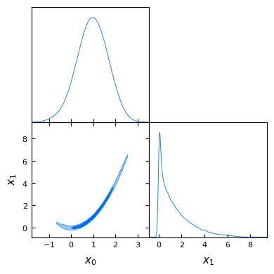
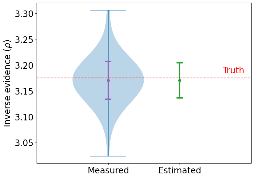
We compute the marginal likelihood for dimension using the learnt harmonic mean estimator and by brute force to provide a ground truth for comparison, evaluating the marginal likelihood by numerical integration (which is possible in this low-dimensional setting). For our learnt harmonic mean estimator, computed using harmonic, we sample the resulting posterior distribution using emcee, drawing 5,000 samples for 200 chains, with burn in of 2,000 samples, yielding 3,000 posterior samples per chain. The recovered posterior distribution is illustrated in Fig. 1. We use 50% of the samples to fit a KDE model for the target distribution (recall that the KDE model is well-suited to problems with narrow curving degeneracies), using cross-validation to estimate the model hyperparameters. The remaining 50% of posterior samples are used to infer the marginal likelihood. Computation time is about one minute to compute on a standard laptop, including drawing all samples and performing cross-validation. We repeat this experiment 100 times in order to estimate the variance of the estimator and its variance, in order to compare to the variance and variance-of-variance estimators described in Sec. 3.2.
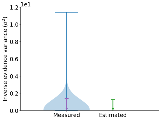
The distribution of marginal likelihood values compute by our learnt harmonic mean estimator for all 100 experiments are shown in Fig. 2. In addition, we show the values computed by the variance and variance-of-variance estimators (estimated) and compare them to the corresponding statistics measured from the 100 experiments (measured). Moreover, we plot the ground truth value computed by numerical integration. The marginal likelihood value computed is in close agreement with the ground truth and the variance and variance-of-variance estimators are in close agreement with the values computed from the experiments. It is clear that the learnt harmonic mean estimator is highly accurate, its variance is well-behaved and its error estimators are also highly accurate.

4.2 Rastrigin
Another common benchmark problem to test marginal likelihood estimators is a likelihood specified by the Rastrigin function. The Rastrigin function exhibits multiple local peaks, which makes it challenging to explore the resulting posterior sufficiently to evaluate the marginal likelihood accurately.
The Rastrigin function is given by
| (73) |
where denotes dimension. Due to its highly multimodal behaviour, it can be difficult to numerically estimate the minimum of the Rastrigin function. Its local minima are given by integer coordinate values, with the global minimum at . We consider a log-likelihood given by and consider a simple uniform prior with for .
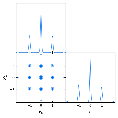
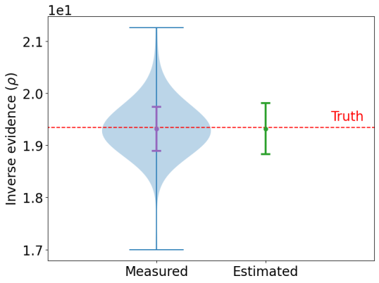
We compute the marginal likelihood for dimension in an identical manner as for the Rosenbrock example, that is, using the learnt harmonic mean estimator and by brute force to provide a ground truth for comparison, evaluating the marginal likelihood by numerical integration (which, again, is possible in this low-dimensional setting). For our learnt harmonic mean estimator, computed using harmonic, we sample the resulting posterior distribution using emcee, drawing 5,000 samples for 200 chains, with burn in of 2,000 samples, yielding 3,000 posterior samples per chain. The recovered posterior distribution is illustrated in Fig. 3. We again adopt a KDE model for the target distribution, avoiding the need to estimate the number of modes in the distribution, and use 50% of the samples to fit the model, using cross-validation to estimate the model hyperparameters. The remaining 50% of posterior samples are used to infer the marginal likelihood. Computation time is about one minute to compute on a standard laptop, including drawing all samples and performing cross-validation. We again repeat this experiment 100 times in order to estimate the variance of the estimator and its variance, in order to compare to the variance and variance-of-variance estimators.
The distribution of marginal likelihood values computed by our learnt harmonic mean estimator for all 100 experiments are shown in Fig. 4. As before, we also show the values computed by the variance and variance-of-variance estimators (estimated) and compare them to the corresponding statistics measured from the 100 experiments (measured). Moreover, we plot the ground truth value computed by numerical integration. It is again clear that the learnt harmonic mean estimator is highly accurate, its variance is well-behaved and its error estimators are also highly accurate.
4.3 Normal-Gamma
An analytically tractable numerical example is considered in Friel and Wyse (2012) to assess the sensitivity of marginal likelihood estimators to changes in the prior. In this study Friel and Wyse (2012) found that the marginal likelihood values computed by the original harmonic mean estimator do not vary with the prior as the values computed analytically do, highlighting this example as a pathological failure of the original harmonic mean estimator. We consider the same pathological example here and demonstrate that our learnt harmonic mean estimator is highly accurate.
We consider the Normal-Gamma model (Bernardo and Smith, 1994) with data
| (74) |
for , with mean and precision (inverse variance) . A normal prior is assumed for and a Gamma prior for :
| (75) | ||||
| (76) |
with mean , shape and rate . The precision scale factor is varied to observe the impact of changing prior on the computed marginal likelihood. The joint prior for then reads:
| (77) | ||||
| (78) |
The likelihood is given by
| (79) | ||||
| (80) | ||||
| (81) | ||||
| (82) |
where ,
| (83) |
and
| (84) |
A graphical representation of the Normal-Gamma model is illustrated in Fig. 5.
For the Normal-Gamma model the marginal likelihood may be computed analytically by
| (85) |
where
| (86) |
| (87) |
and
| (88) | ||||
| (89) |
To assess the impact of altering the prior, we compute the marginal likelihood both analytically and using our learnt harmonic mean estimator for priors corresponding to . Data are simulated with underlying parameters to generate synthetic observations (the same experimental configuration considered by Friel and Wyse 2012).
| Analytic | -144.5530 | -143.4017 | -142.2505 | -141.0999 | -139.9552 |
|---|---|---|---|---|---|
| Estimated | -144.5545 | -143.3990 | -142.2490 | -141.1001 | -139.9558 |
| Error | -0.0015 | 0.0027 | 0.0015 | -0.0011 | -0.0006 |
| (learnt harmonic mean) | |||||
| Error | 12.2100 | — | 9.7900 | 8.5000 | 7.1000 |
| (original harmonic mean) |
For our learnt harmonic mean estimator we use emcee to draw 1,500 samples for 200 chains, with burn in of 500 samples, yielding 1,000 posterior samples per chain. We use 25% of the samples to learn the target model, using cross-validation to select between the hypersphere and modified Gaussian mixture model. In all cases the modified Gaussian mixture model is selected. The remaining 75% of posterior samples are used for inferring the marginal likelihood. Computation time is about one minute on a standard laptop for each experiment (i.e. each ) considered, including drawing all samples.
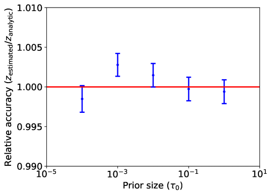
The marginal likelihood values computed analytically and using our learnt harmonic mean estimator are shown in Table 1 for different priors as is varied. For comparison, the errors between the analytic values and those estimated by our learnt harmonic mean estimator and the original harmonic mean estimator are also shown. Notice that the marginal likelihood values computed by the learnt harmonic mean estimator are highly accurate and do indeed vary with differing priors, in contrast to results computed by the original harmonic mean estimator (Friel and Wyse, 2012). The improvement in accuracy between the original and our learnt harmonic mean estimation is approximately four orders of magnitude in log space. In addition, to graphically compare the marginal likelihood values estimated by the learnt harmonic mean estimator to the analytic values, we plot in Fig. 6 the ratio of the estimated and analytic values, with the uncertainties computed by our learnt harmonic mean estimator overlaid. It is clear that the marginal likelihood values computed by the learnt harmonic mean estimator closely estimate the analytic values and that the uncertainties are reasonable.
4.4 Logistic regression models: Pima Indian example
We consider the comparison of two logistic regression models using the Pima Indians data, which is another common benchmark problem for comparing estimators of the marginal likelihood. The original harmonic mean estimator has been shown to fail catastrophically for this example (Friel and Wyse, 2012), whereas we show here that our learnt harmonic mean estimator is highly accurate.
The Pima Indians data (Smith et al, 1988), originally from the National Institute of Diabetes and Digestive and Kidney Diseases, were compiled from a study of indicators of diabetes in Pima Indian women aged 21 or over. Seven primary predictors of diabetes were recorded, including: number of prior pregnancies (NP); plasma glucose concentration (PGC); diastolic blood pressure (BP); triceps skin fold thickness (TST); body mass index (BMI); diabetes pedigree function (DP); and age (AGE).
The probability of diabetes for person can be modelled by the standard logistic function
| (90) |
with covariates and parameters , where is the total number of covariates considered. The likelihood function then reads
| (91) |
where is the diabetes incidence, i.e. is unity if patient has diabetes and zero otherwise. An independent multivariate Gaussian prior is assumed for the parameters , given by
| (92) |
with precision .
Two different logistic regression models are considered, with different subsets of covariates:
| covariates = {NP, PGC, BMI, DP} (and bias); | |||
| covariates = {NP, PGC, BMI, DP, AGE} (and bias). |
A graphical representation of Model 2 is illustrated in Fig. 7 (Model 1 is similar but does not include the AGE covariate).
We compute the marginal likelihood for both Model 1 and Model 2 using our learnt harmonic mean estimator for and , as in Friel and Wyse (2012). A reversible jump algorithm (Green, 1995) is used by Friel and Wyse (2012) to compute benchmark Bayes factors of 13.96 and 1.30, respectively, for and , which are treated as ground truth values.
For our learnt harmonic mean estimator we use emcee to draw 5,000 samples for 200 chains, with burn in of 1,000 samples, yielding 4,000 posterior samples per chain. We use 25% of the samples to learn the target model, using cross-validation to select between the hypersphere and modified Gaussian mixture model. In all cases the modified Gaussian mixture model is selected. The remaining 75% of posterior samples are used for inferring the marginal likelihood. Computation time is typically a few minutes on a standard laptop, including drawing samples (note that fewer samples could likely be used to reduce computation time if required).
The marginal likelihood values computed by our learnt harmonic mean estimator are shown in Table 2 and Table 3 for the cases and , respectively. The benchmark values and errors of both the standard and learnt harmonic mean estimator are also shown for comparison. While the standard harmonic mean estimator fails catastrophically on this problem (Friel and Wyse, 2012), our learnt harmonic mean estimator is robust and highly accurate.
| Model | Model | ||
| Benchmark | – | – | 2.63620 |
| Estimated | -257.23656 | -259.86669 | 2.63014 |
| 0.00264 | 0.00968 | 0.01232 | |
| Error | – | – | 0.00606 |
| (learnt harmonic mean) | |||
| Error | – | – | -2.67760 |
| (original harmonic mean) |
| Model | Model | ||
| Benchmark | – | – | 0.26236 |
| Estimated | -247.30633 | -247.56128 | 0.25495 |
| 0.00239 | 0.00789 | 0.01028 | |
| Error | – | – | 0.00742 |
| (learnt harmonic mean) | |||
| Error | – | – | -0.44567 |
| (original harmonic mean) |
4.5 Non-nested linear regression models: Radiata pine example
We consider another example where the original harmonic mean estimator was shown to fail catastrophically (Friel and Wyse, 2012). In particular, we consider non-nested linear regression models for the Radiata pine data, which is another common benchmark data-set (Williams, 1959), and show that our learnt harmonic mean estimator is highly accurate.
For trees, the Radiata pine data-set includes measurements of the maximum compression strength parallel to the grain , density and resin-adjusted density , for specimen . The question at hand is whether density or resin-adjusted density is a better predictor of compression strength. This motivates two Gaussian linear regression models:
| (93) | ||||||||
| (94) |
where , , and and denote the precision (inverse variance) of the noise for the respective models.
For Model 1, Gaussian priors are assumed for the bias and linear terms:
| (95) | ||||
| (96) |
with means and , and precision scales and . A gamma prior is assumed for the noise precision:
| (97) |
with shape and rate . The joint prior for then reads:
| (98) | ||||
| (99) | ||||
| (100) |
The likelihood for Model 1 is given by
| (101) | ||||
| (102) | ||||
| (103) |
where and . For Model 2, the priors adopted for are the same as those adopted for of Model 1, respectively, with the same hyperparameters. The likelihood for Model 2 again takes an identical form to Model 1. A graphical representation of Model 1 is illustrated in Fig. 8 (Model 2 is similar).
One reason this problem has become a common benchmark for comparing marginal likelihood estimators is that the marginal likelihood of the two models can be computed analytically. The evidence for Model 1 is given by
| (104) |
where , , , and , for the feature matrix with row containing .
We compute the marginal likelihood analytically using (104) and also numerically using our learnt harmonic mean estimator. For the learnt harmonic mean estimator we use emcee to draw 20,000 samples for 400 chains, with burn in of 2,000 samples. We use 25% of the samples to learn the target model, adopting a simple hypersphere model, and use the remaining 75% for inferring the marginal likelihood. Computation time is a few minutes on a standard laptop, including drawing samples (note that fewer samples could likely be used to reduce computation time if required).
The analytic and estimated marginal likelihood values are shown in Table 4 for the two models, with the Bayes factor comparing the two models. For the values computed by our learnt harmonic mean estimator we also show the estimated uncertainty. The errors of both the standard and learnt harmonic mean estimator are shown for comparison. Note that the uncertainties estimated by the learnt harmonic mean estimator appear reasonable. While the standard harmonic mean estimator fails catastrophically on this problem (Friel and Wyse, 2012), our learnt harmonic mean estimator is highly accurate.
| Model | Model | ||
| Analytic | -310.12829 | -301.70460 | 8.42368 |
| Estimated | -310.12807 | -301.70413 | 8.42394 |
| 0.00072 | 0.00074 | 0.00145 | |
| Error | 0.00022 | 0.00047 | 0.00026 |
| (learnt harmonic mean) | |||
| Error | – | – | -0.17372 |
| (original harmonic mean) |
4.6 Gaussian in varying dimensions
Finally, we illustrate the application of our estimator beyond low-dimensional settings, considering experiments where the dimension of the parameter space increases. For simplicity we consider a Gaussian likelihood with a uniform prior, where the marginal likelihood can be computed analytically. We adopt the simple hypersphere model, which is effective for a Gaussian posterior. Results are illustrated in Table 5. Note that parameters were not optimised and accurate results could likely be obtained with fewer samples. Further note that the computation times recorded do not include the time accumulated during initial burn-in. It is apparent that the estimator is accurate in settings with dimensions and potentially beyond.
| Dimension | Analytic | Estimated | Error | Computation |
|---|---|---|---|---|
| (%) | time | |||
| 32 | -29.406 | -29.411 | 0.0180% | 10 sec |
| 64 | -58.812 | -58.813 | 0.0008% | 20 sec |
| 128 | -117.62 | -117.63 | 0.0026% | 3 min |
| 256 | -235.25 | -235.25 | 0.0015% | 18 min |
| 512 | -470.50 | -470.49 | 0.0006% | 20 min |
| 1024 | -940.99 | -941.06 | 0.0073% | 3 hours |
4.7 Cosmological example
We conclude our numerical experiments with an application of the learnt harmonic mean estimator to a model comparison problem in cosmology. We consider measurements of the Cosmic Microwave Background (CMB) temperature () and polarisation () anisotropies from Data Release 4 of the Atacama Cosmology Telescope (ACT) (Aiola et al, 2020; Choi et al, 2020).
The dataset consists of CMB power spectra , with measured at angular multipoles up to 5000. CMB power spectra are functions of the cosmological parameters that describe the model assumed for the composition and evolution of the Universe. The Cold Dark Matter (CDM) model is currently regarded as the concordance cosmological scenario, as it provides an excellent fit to numerous cosmological measurements. However, some of its key components are poorly understood, including the cosmological constant that gives its name to the model and is deemed responsible for the accelerated expansion of the Universe. Alternative models have been proposed to account for cosmic acceleration. One of them attributes this phenomenon to a dynamic dark energy component – a fluid whose equation of state (the relation between its pressure and density ) changes over time. Using redshift as a proxy for cosmic time (with today), this can be written as . A common parameterisation for is (Chevallier and Polarski, 2001; Linder, 2003), with and corresponding to a cosmological constant. Thus, the CDM model can be seen as an extension to the CDM model, to account for cosmic acceleration through a dynamic dark energy field which introduces two additional cosmological parameters in the model, and .
We aim to perform a comparison between the CDM and CDM models using ACT CMB data. We employ the learnt harmonic mean estimator to derive estimates of the Bayesian evidence for each model, and the Bayes factor between the two. We then compare these numbers against those obtained with an independent approach, namely a nested sampler which produces an estimate of the evidence as well as posterior samples for each model. To run our experiments we use the publicly available pyactlike likelihood 444https://github.com/ACTCollaboration/pyactlike/, developed by the ACT collaboration to analyse their CMB power spectra measurements. This likelihood only includes one additional ‘nuisance’ parameter, , to the cosmological parameters underlying the model of the Universe. This parameter acts as a phenomenological rescaling of the spectra to account for undetected systematics. Table 6 shows the priors assumed for all of the parameters varied in the analysis. Priors on all parameters are shared between the emcee and PolyChord runs, with the exception of and used only in the dynamic dark energy scenario.
We compare two experimental setups:
-
1.
In the first one, we use the affine sampler emcee (Foreman-Mackey et al, 2013) to produce 30,000 samples of the posterior, using 300 walkers each collecting 150 samples, of which we discard 50 for each walker as burn-in. We run the sampler on a 60-core parallelised configuration, which takes approximately 5 hours to complete. Once obtained the posterior samples, we use our implementation of the learnt harmonic mean estimator to derive an estimate of the evidence for each of the two cosmological models. We use the hypersphere model for the learnt harmonic mean estimator in both cosmological scenarios, and perform a 50:50 split of the posterior samples for the training and testing phase.
-
2.
In the second setup, we run the nested sampler PolyChord (Handley et al, 2015b, a) to obtain posterior samples and an estimate of the evidence for each model. We run PolyChord through the Cobaya (Torrado and Lewis, 2021, 2019) software for cosmological data analysis. We use the same parallelised configuration over 60 cores used for the emcee runs, and default values for the PolyChord options. This leads to and samples for the CDM and CDM model, respectively, obtained in 15 hours for both cases.
| Parameter | Prior |
|---|---|
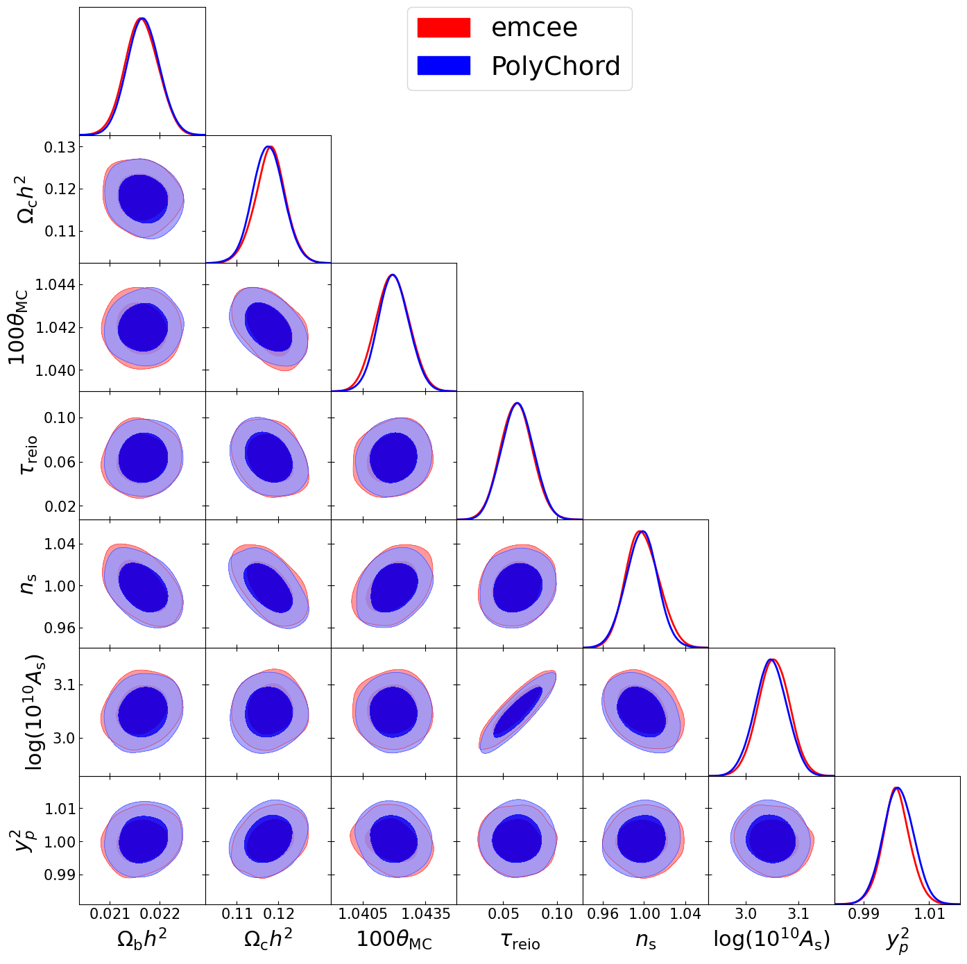
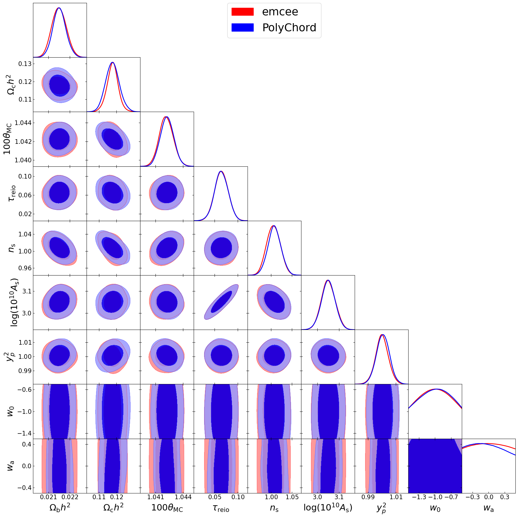
Fig. 9 and 10 show the posterior contours for the CDM and CDM model, respectively. Each figure compares contours obtained with the emcee (red) and PolyChord (blue) sampler. For the CDM runs, we obtain a value of the log-evidence
| (105) |
while for CDM we obtain
| (106) |
Combined, these measurements lead to a Bayes factor
| (107) |
We can see from these results that the learnt harmonic mean estimator leads to numerical conclusions on the comparison between the CDM and CDM models in excellent agreement with those derived from running PolyChord, i.e. mildly favouring CDM. Note also that by virtue of its independence from the sampling method, the learnt harmonic mean estimator allows the user to resort to the emcee sampler which leads to 3 to 6 times more samples than PolyChord in 1/3 of the time, using the same hardware resources.
5 Software package
The learnt harmonic mean estimator is implemented in the harmonic software package555https://github.com/astro-informatics/harmonic, which is open source and publicly available. Careful consideration has been given to the design and implementation of the code, following software engineer best practices (for example, at the time of release test coverage is over 96%).
Since the learnt harmonic mean estimator requires samples from the posterior distribution only, the harmonic code is agnostic to the method or code used to generate posterior samples. That said, harmonic works exceptionally well with MCMC sampling techniques that naturally provide samples from multiple chains by their ensemble nature, such as affine invariance ensemble samplers (Goodman and Weare, 2010). As discussed in Sec. 2, we advocate running a number of independent MCMC chains and using all of the correlated samples within a chain to avoid the loss of efficiency that otherwise results from thinning an MCMC chain. The emcee code666https://emcee.readthedocs.io/en/stable/ (Foreman-Mackey et al, 2013) provides an excellent implementation of the affine invariance ensemble samplers proposed by Goodman and Weare (2010). emcee is thus a natural choice for use with harmonic and we have specifically designed harmonic to ensure it works seamlessly with emcee (although of course other samplers can also be considered). In code Listing 1 we give an example of usage of harmonic with emcee to demonstrate how easy it is to use the combination for marginal likelihood estimation.
6 Conclusions
We present the learnt harmonic mean estimator to solve the problematic large variance of the original estimator. The construction of our estimator follows by interpreting the harmonic mean estimator as importance sampling and introducing a new target distribution that is learned to approximate the optimal but inaccessible target (the normalised posterior), while minimising the variance of the resulting estimator. We discuss techniques to compute the variance of the estimator, its variance and to perform a number of additional computational sanity checks. The estimator is implemented in the publicly available harmonic software code. We demonstrate the application of our learnt harmonic mean estimator on numerous benchmark problems, including a number of pathological examples where the original harmonic mean estimator fails catastrophically. In all cases our estimator is robust and highly accurate. The current work opens up a number of avenues for future research. For example, similar approaches can be taken in MCMC sampling more generally were appropriate target, sampling densities or proposal distributions may be learned. Alternative more effective target models can be developed that better scale to higher dimensional settings. Since the learnt harmonic mean estimator is agnostic to the sampling strategy, it is also an ideal solution for computing the marginal likelihood for model comparison in simulation-based inference. We are already actively pursuing this avenue of research, with promising preliminary results.
Acknowledgments
This work was supported by the Leverhulme Trust and by EPSRC grant EP/W007673/1. For the purpose of open access, the authors have applied a Creative Commons Attribution (CC BY) licence to any Author Accepted Manuscript version arising.
References
- \bibcommenthead
- Aiola et al (2020) Aiola S, Calabrese E, Maurin L, et al (2020) The atacama cosmology telescope: DR4 maps and cosmological parameters. Journal of Cosmology and Astroparticle Physics 2020(12):047–047. 10.1088/1475-7516/2020/12/047, URL https://doi.org/10.1088%2F1475-7516%2F2020%2F12%2F047
- Bernardo and Smith (1994) Bernardo J, Smith A (1994) Bayesian theory. Wiley Online Library https://doi.org/10.1002/9780470316870.ch5
- Brewer et al (2011) Brewer BJ, Pártay LB, Csányi G (2011) Diffusive nested sampling. Statistics and Computing 21:649–656
- Cai et al (2021) Cai X, McEwen JD, Pereyra M (2021) High-dimensional Bayesian model selection by proximal nested sampling. SIAM Journal on Imaging Sciences, submitted https://arxiv.org/abs/arXiv:2106.03646
- Chevallier and Polarski (2001) Chevallier M, Polarski D (2001) Accelerating universes with scaling dark matter. International Journal of Modern Physics D 10(02):213–223. 10.1142/s0218271801000822, URL https://doi.org/10.1142%2Fs0218271801000822
- Chib (1995) Chib S (1995) Marginal likelihood from the gibbs output. Journal of the American Statistical Association 90(432):1313–1321
- Chib and Jeliazkov (2001) Chib S, Jeliazkov I (2001) Marginal likelihood from the Metropolis-Hastings output. Journal of the American Statistical Association 96:270–281
- Cho et al (2005) Cho E, Cho MJ, Eltinge J (2005) The variance of sample variance from a finite population. International Journal of Pure and Applied Mathematics 21(3):389
- Choi et al (2020) Choi SK, Hasselfield M, Ho SPP, et al (2020) The atacama cosmology telescope: a measurement of the cosmic microwave background power spectra at 98 and 150 GHz. Journal of Cosmology and Astroparticle Physics 2020(12):045–045. 10.1088/1475-7516/2020/12/045, URL https://doi.org/10.1088%2F1475-7516%2F2020%2F12%2F045
- Clyde et al (2007) Clyde M, Berger J, Bullard F, et al (2007) Current challenges in bayesian model choice. In: Statistical challenges in modern astronomy IV, p 224
- Feroz and Hobson (2008) Feroz F, Hobson MP (2008) Multimodal nested sampling: an efficient and robust alternative to Markov Chain Monte Carlo methods for astronomical data analyses. Mon Not Roy Astron Soc 384:449–463. 10.1111/j.1365-2966.2007.12353.x, https://arxiv.org/abs/arXiv:arXiv:0704.3704
- Feroz et al (2009) Feroz F, Hobson MP, Bridges M (2009) MultiNest: an efficient and robust bayesian inference tool for cosmology and particle physics. Mon Not Roy Astron Soc 398:1601–1614. 10.1111/j.1365-2966.2009.14548.x, https://arxiv.org/abs/arXiv:arXiv:0809.3437
- Foreman-Mackey et al (2013) Foreman-Mackey D, Hogg DW, Lang D, et al (2013) emcee: The mcmc hammer. PASP 125:306–312. 10.1086/670067, https://arxiv.org/abs/1202.3665
- Foreman-Mackey et al (2013) Foreman-Mackey D, Hogg DW, Lang D, et al (2013) emcee: The MCMC hammer. Publications of the Astronomical Society of the Pacific 125(925):306–312. 10.1086/670067, URL https://doi.org/10.1086%2F670067
- Friel and Wyse (2012) Friel N, Wyse J (2012) Estimating the evidence – a review. Statistica Neerlandica 66(3):288–308. 10.1111/j.1467-9574.2011.00515.x, URL http://dx.doi.org/10.1111/j.1467-9574.2011.00515.x, https://arxiv.org/abs/arXiv:arXiv:1111.1957
- Gelfand and Dey (1994) Gelfand AE, Dey DK (1994) Bayesian model choice: asymptotics and exact calculations. Journal of the Royal Statistical Society: Series B (Methodological) 56(3):501–514
- Goodman and Weare (2010) Goodman J, Weare J (2010) Ensemble samplers with affine invariance. Communications in applied mathematics and computational science 5(1):65–80
- Green (1995) Green PJ (1995) Reversible jump markov chain monte carlo computation and bayesian model determination. Biometrika 82(4):711–732
- van Haasteren (2014) van Haasteren R (2014) Marginal likelihood calculation with mcmc methods. In: Gravitational Wave Detection and Data Analysis for Pulsar Timing Arrays. Springer, p 99–120
- Handley et al (2015) Handley WJ, Hobson MP, Lasenby AN (2015) POLYCHORD: nested sampling for cosmology. Mon Not Roy Astron Soc 450:L61–L65. 10.1093/mnrasl/slv047, https://arxiv.org/abs/arXiv:arXiv:1502.01856
- Handley et al (2015a) Handley WJ, Hobson MP, Lasenby AN (2015a) polychord: nested sampling for cosmology. Monthly Notices of the Royal Astronomical Society: Letters 450(1):L61–L65. 10.1093/mnrasl/slv047, URL https://doi.org/10.1093%2Fmnrasl%2Fslv047
- Handley et al (2015b) Handley WJ, Hobson MP, Lasenby AN (2015b) polychord: next-generation nested sampling. Monthly Notices of the Royal Astronomical Society 453(4):4385–4399. 10.1093/mnras/stv1911, URL https://doi.org/10.1093%2Fmnras%2Fstv1911
- Hastings (1970) Hastings WK (1970) Monte Carlo sampling methods using Markov chains and their applications. Biometrika 57:97–109
- Heavens et al (2017) Heavens A, Fantaye Y, Mootoovaloo A, et al (2017) Marginal likelihoods from Monte Carlo Markov Chains. ArXiv https://arxiv.org/abs/arXiv:arXiv:1704.03472
- Lenk (2009) Lenk P (2009) Simulation pseudo-bias correction to the harmonic mean estimator of integrated likelihoods. Journal of Computational and Graphical Statistics 18(4):941–960
- Linder (2003) Linder EV (2003) Exploring the expansion history of the universe. Phys Rev Lett 90:091,301. 10.1103/PhysRevLett.90.091301, URL https://link.aps.org/doi/10.1103/PhysRevLett.90.091301
- Link and Eaton (2012) Link WA, Eaton MJ (2012) On thinning of chains in mcmc. Methods in ecology and evolution 3(1):112–115
- Marshall et al (2003) Marshall PJ, Hobson MP, Slosar A (2003) Bayesian joint analysis of cluster weak lensing and Sunyaev-Zel’dovich effect data. Mon Not Roy Astron Soc 346:489–500
- Metropolis et al (1953) Metropolis N, Rosenbluth AW, Rosenbluth MN, et al (1953) Equation of state by fast computing machines. J Chemical Physics 21:1087–1092
- Neal (2001) Neal R (2001) Annealed importance sampling. Statistics and Computing 11:125–139
- Neal (1994) Neal RM (1994) Contribution to the discussion of “Approximate Bayesian inference with the weighted likelihood bootstrap” by Newton MA, Raftery AE. JR Stat Soc Ser A (Methodological) 56:41–42
- Newton and Raftery (1994) Newton MA, Raftery AE (1994) Approximate Bayesian inference with the weighted likelihood bootstrap. Journal of the Royal Statistical Society Series B (Methodological) 56(1):3–48. URL http://www.jstor.org/stable/2346025
- O’Ruanaidh and Fitzgerald (1996) O’Ruanaidh J, Fitzgerald WJ (1996) Numerical Bayesian methods applied to signal processing. Springer-Verlag New York
- Pajor et al (2017) Pajor A, et al (2017) Estimating the marginal likelihood using the arithmetic mean identity. Bayesian Analysis 12(1):261–287
- Robert and Wraith (2009) Robert CP, Wraith D (2009) Computational methods for Bayesian model choice. In: Aip conference proceedings, American Institute of Physics, pp 251–262
- Rose and Smith (2002) Rose C, Smith MD (2002) Mathstatica: mathematical statistics with mathematica. In: Compstat, Springer, pp 437–442
- Skilling (2006) Skilling J (2006) Nested sampling for general Bayesian computation. Bayesian Analysis 1:833–859
- Smith et al (1988) Smith JW, Everhart JE, Dickson W, et al (1988) Using the adap learning algorithm to forecast the onset of diabetes mellitus. In: Proceedings of the annual symposium on computer application in medical care, American Medical Informatics Association, p 261
- Tierney and Kadane (1986) Tierney L, Kadane JB (1986) Accurate approximations for posterior moments and marginal densities. Journal of the American Statistical Association 81:82–86
- Torrado and Lewis (2019) Torrado J, Lewis A (2019) Cobaya: Bayesian analysis in cosmology. Astrophysics Source Code Library, record ascl:1910.019, 1910.019
- Torrado and Lewis (2021) Torrado J, Lewis A (2021) Cobaya: code for bayesian analysis of hierarchical physical models. Journal of Cosmology and Astroparticle Physics 2021(05):057. 10.1088/1475-7516/2021/05/057, URL https://doi.org/10.1088%2F1475-7516%2F2021%2F05%2F057
- Trotta (2007) Trotta R (2007) Applications of Bayesian model selection to cosmological parameters. Mon Not Roy Astron Soc 378:72–82
- Williams (1959) Williams EJ (1959) Regression analysis. Wiley, New York