Direct implementation of a perceptron in superconducting circuit quantum hardware

Abstract

The utility of classical neural networks as universal approximators suggests that their quantum analogues could play an important role in quantum generalizations of machine-learning methods. Inspired by the proposal in Torrontegui and García-Ripoll (2019), we demonstrate a superconducting qubit implementation of an adiabatic controlled gate, which generalizes the action of a classical perceptron as the basic building block of a quantum neural network. We show full control over the steepness of the perceptron activation function, the input weight and the bias by tuning the adiabatic gate length, the coupling between the qubits and the frequency of the applied drive, respectively. In its general form, the gate realizes a multi-qubit entangling operation in a single step, whose decomposition into single- and two-qubit gates would require a number of gates that is exponential in the number of qubits. Its demonstrated direct implementation as perceptron in quantum hardware may therefore lead to more powerful quantum neural networks when combined with suitable additional standard gates.

I Introduction

Artificial neural networks and engineered quantum systems are both quickly developing technologies with far-reaching potential applications. The promise that quantum computing can solve certain problems exponentially faster than classical computing technology and the ever growing thirst for computational power of machine learning applications has triggered substantial interest in the development of quantum machine learning methodology Biamonte et al. (2017); Rocchetto et al. (2018); Das Sarma et al. (2019); Zoufal et al. (2019); Melko et al. (2019); Abbas et al. (2021); Havlíček et al. (2019); Glick et al. (2021). Whereas some work explored the acceleration of specific computational tasks in machine learning with quantum encodings Harrow et al. (2009), a major part of the research considers quantum neural networks as counterparts to artifical neural networks in classical software. Quantum neural networks are largely implemented as variational quantum circuits Farhi et al. (2014); Peruzzo et al. (2014); Moll et al. (2018); Kandala et al. (2017), that are composed of parametrized gates and where finding optimal parameters corresponds to the training of the network. Moreover, it has been shown that quantum speed-up is possible in supervised machine learning Liu et al. (2021), providing a perspective for hardware-efficient machine learning realizations.

An important question for quantum neural networks is their expressivity, i.e. which mappings between input and output states can be realized by the network. In the classical domain, expressivity is guaranteed by the universal approximation theorem, which requires a nonlinear activation function for the perceptrons in the network. In the quantum setting, it has been shown that similar notions of universal approximation exist for functions mapping gate parameters to the state prepared by the quantum circuit Pérez-Salinas et al. (2021). However, currently there is no universally accepted way to extend the concept of classical neural networks to quantum systems Behrman et al. (2000); Schuld et al. (2014). One option is to design a quantum perceptron as a unitary whose action on a set of basis states matches a classical perceptron Torrontegui and García-Ripoll (2019). Such a building block can serve as a tool to enable experimental studies and development of quantum neural networks. Since such an approach includes the functionality of classical neural networks in limiting cases, it has the expressive power guaranteed by the universal approximation theorem in those cases and thus forms a natural starting point for exploring quantum generalizations. Another advantage of this approach is that the perceptron may be directly realized at the hardware level, rather than encoded in software: this neuromorphic approach is more hardware efficient and may thus offer significant advantages for scaling the concept to larger and more data intensive applications.

The construction of the quantum counterpart to a perceptron is easily illustrated with the example of a binary classifier perceptron. This simple classical perceptron takes a number of binary inputs $x_{i}\in\{0,1\}$, each with an associated weight $w_{i}$, and outputs another binary value $y$ depending on whether the linear combination $x_{\text{in}}=w_{1}x_{1}+\ldots$ exceeds a given threshold or not:

$$y=\left\{\begin{array}[]{l}0\text{ if }x_{\text{in}}+b<0\\ 1\text{ if }x_{\text{in}}+b\geq 0\\ \end{array}\right.,$$

or, written compactly in terms of the Heaviside step function, $y=\Theta(x_{\text{in}}+b)$ with an additional bias $b$. More generally, as illustrated in Fig. 1(a), the step function may be replaced by a continuous activation function $f$ and the inputs and outputs promoted from binary values to continuous ones. The key advantage of such continuous activation functions is that they have finite gradients which can be used for training the network in gradient descent approaches.

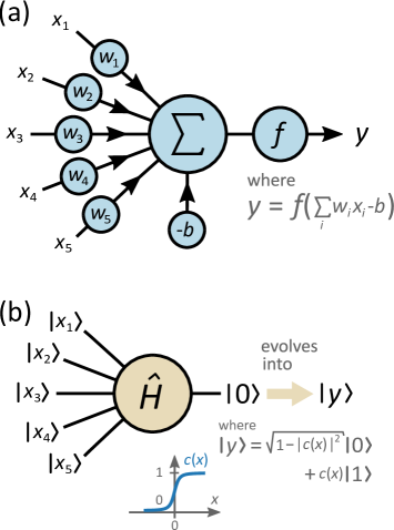
Figure 1: (a) Schematic representation of a classical perceptron with $n=5$ inputs. The perceptron output $y$ is given by a non-linear activation function $f(\cdot)$ applied to the sum of input values $x_{1},...,x_{n}$ individually weighted by $w_{1},...,w_{n}$ and biased by a term $b$. A quantum analog (b) can be constructed, where the inputs are encoded in quantum states $\ket{x_{1}},...,\ket{x_{n}}$ of $n$ qubits and an output qubit undergoes a rotation by an angle of $\theta=\arcsin[c(x)]$ determined by the inputs values, leading to an excited population of $|c(x)|^{2}$ when starting the output qubit in the ground state.

In a quantum generalization of the classifier perceptron, the binary variables can be naturally represented by qubit states, which we will label as $|0\rangle$ and $|1\rangle$. The action of the perceptron can then be represented by a gate $U$ whose effect on the output qubit depends on the states of the input qubits:

$$|x_{1}x_{2}\ldots\rangle_{\mathrm{in}}\otimes|0\rangle_{\mathrm{out}}\xrightarrow{U}\left\{\begin{array}[]{l}|x_{1}x_{2}\ldots\rangle_{\mathrm{in}}\otimes|0\rangle_{\mathrm{out}}\\ \text{ if }x_{\text{in}}+b\equiv\sum_{j}w_{j}x_{j}+b<0\\ \\ |x_{1}x_{2}\ldots\rangle_{\mathrm{in}}\otimes|1\rangle_{\mathrm{out}}\\ \text{ if }x_{\text{in}}+b\equiv\sum_{j}w_{j}x_{j}+b\geq 0\\ \end{array}\right.$$

When the input is a product state $|x_{1}x_{2}\ldots\rangle_{\mathrm{in}}$, then the unitary is simply a rotation of the output qubit by $0$ or $\pi$ depending on the sign of $x_{\text{in}}+b$ Cao et al. (2017). This concept of a quantum perceptron can be further generalized, similarly to the classical case, by letting the rotation angle have a different dependence on $x$ than a simple Heaviside function. The action of the perceptron, shown schematically in Fig. 1(b), is then described as

$$|x_{1}x_{2}\ldots\rangle_{\mathrm{in}}\otimes|0\rangle_{\mathrm{out}} \xrightarrow{U}|x_{1}x_{2}\ldots\rangle_{\mathrm{in}}\otimes|y\rangle_{\mathrm{out}},$$

$$\text{where }|y\rangle_{\mathrm{out}} =\sqrt{1-|c(x)|^{2}}|0\rangle+c(x)|1\rangle.$$ (1)

Here the excitation amplitude $c(x)$ is a continuous, step-like function of $x\equiv x_{\text{in}}+b$ such as depicted in Fig. 1. The previously described binary perceptron is the special case where $c(x)$ is the Heaviside step function $\Theta(x)$.

Since the perceptron gate is a unitary operation, it can in principle be implemented via any universal set of quantum gates, such as single-qubit rotations and controlled-NOT (CNOT) gates. However, the depth of such a decomposition in general grows exponentially in the number of input qubits. Therefore, we instead realize the perceptron gate directly, making use of an adiabatic protocol. This approach allows us to implement the gate with a single adiabatic pulse whose duration does not scale with the number of input qubits: From Eq. (1) it can be seen that the perceptron acts like a multi-qubit controlled gate. However, instead of triggering an operation on the target only when the control register is in the $\ket{1\dots 1}$ state (like a Toffoli gate Fredkin and Toffoli (1982), which applies an $X$ gate to the target only when the control qubits are in the state $\ket{11}$), the perceptron gate applies a different operation to the output qubit for each possible input basis state $\ket{x_{1}x_{2}\dots}_{\textrm{in}}$. As the number of input basis states grows exponentially in the number of qubits, a standard decomposition into elementary gates leads to an expontial growth of the circuit depth (see Section III), which is in contrast to the adiabatic implementation discussed in the following.

II The perceptron gate

II.1 Concept

We construct the perceptron unitary with an approach that is a slight modification of a theoretical proposal by Torrontegui and García-Ripoll Torrontegui and García-Ripoll (2019), as described below. An implementation of a similar operation was also proposed Cao et al. (2017) based on repeated measurements and feedback, while a gate-based approach to construction of activation functions was demonstrated in Yan et al. (2020).

Our protocol, which we implement in a device with two fixed-frequency superconducting transmon qubits Koch et al. (2007) interacting via a tunable coupler McKay et al. (2016) (schematically depicted in Fig. 2(a)) is based on an adiabatic unitary evolution applied to the output qubit. This gate $U_{\mathrm{ad}}$ is designed in such a way that the final excited state amplitude depends on the detuning $\Delta$ of a microwave drive frequency from the output qubit frequency via the step-like response function $c(\Delta)$:

$$|0\rangle_{\mathrm{out}}\xrightarrow{U_{\mathrm{ad}}}\sqrt{1-|c(\Delta)|^{2}}|0\rangle_{\mathrm{out}}+c(\Delta)|1\rangle_{\mathrm{out}}$$ (2)

Note that this becomes exactly the mapping in Eq. (1) if the detuning $\Delta$ is equal to the linear combination of inputs $\sum_{j}w_{j}x_{j}+b$. We achieve this linear dependence of $\Delta$ on the input states by subjecting the system to a $ZZ$ interaction between each of the input qubits and the perceptron qubit:

$$H_{\mathrm{int}}=-\sum_{j}w_{j}|1\rangle\langle 1|_{j}\otimes|1\rangle\langle 1|_{\mathrm{out}}$$ (3)

Here $j$ enumerates the input qubits and "$\mathrm{out}$" labels the output qubit. If the input qubits are in a product state $|x_{1}\ldots\rangle$, this is equivalent to shifting the frequency of the output by $-\sum_{j}w_{j}x_{j}$, or $-w_{1}x_{1}$ in the case of a single input.

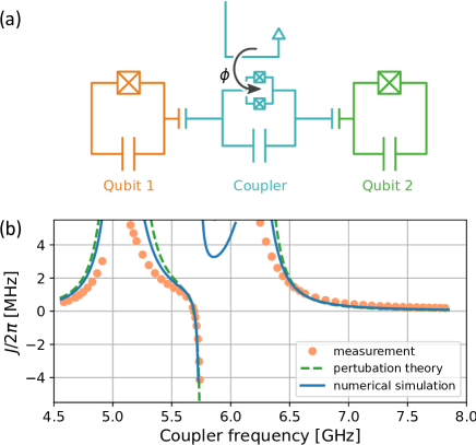
Figure 2: (a) Diagram of the two-qubit experimental setup: two fixed frequency transmons are capacitively coupled via a flux-tunable coupler whose frequency determines the ZZ coupling between the qubits. (b) Measured value of the ZZ coupling as a function of the tunable coupler’s frequency (orange dots). Here we plot the coupling strength $J$ conventionally defined via $H_{\mathrm{int}}=J|11\rangle\langle 11|$. In the perceptron context, the weight $w$ from Eq. (3) is given by $w=-J$. The solid line is the result of numerically diagonalizing the hamiltonian of the system and the dashed line is the result of the lowest order perturbative calculation (Appendix B).

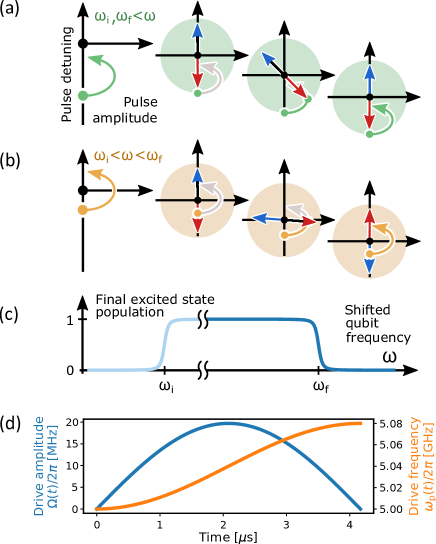
Figure 3: (a,b) Illustration of the effect of an adiabatic chirped pulse with initial and final frequencies $\omega_{\mathrm{i}}$ and $\omega_{\mathrm{f}}$ on a qubit with a frequency $\omega$. (a) If the initial and final detunings have the same sign, the basis states $|0\rangle$ and $|1\rangle$ are unchanged (up to a phase). (b) If the signs are opposite, the states get swapped. This results in a dependence of the final state on the shifted qubit frequency shown in (c). The perceptron activation function is realized by this dependence in the vicinity of $\omega\approx\omega_{\mathrm{f}}$ (darker line). (d) Time-dependence of the amplitude $\Omega(t)$ and frequency $\omega_{p}(t)$ of an exemplary adiabatic chirped pulse realizing the output-qubit rotation.

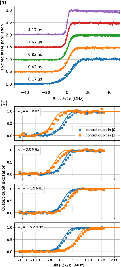
Figure 4: (a) The quantum perceptron activation functions: The excited state population $p_{\mathrm{e}}$ of the output qubit as a function of its final detuning $\Delta$ after an adiabatic chirped pulse is applied on the ground state of two-qubit system. Results for different pulse lengths $T$ are offset for visualization. The characteristic width of the activation function is inversely proportional to the pulse lengths $T$. The solid lines result from a simulation of unitary evolution under the adiabatic drive, with no fit parameters in this model. (b) Frequency shift of the activation function dependent on the state of the input qubit, for a pulse length of $T=1.67\,\mu\mathrm{s}$ Both the magnitude and sign of this shift can be varied by tuning the frequency of the coupler. In these plots, the output qubit excitations are rescaled to correct for relaxation and readout imperfections, in order to highlight the agreement of the curve’s shape with the simulation results. The frequency spacing between the simulated curves is not obtained by fitting but rather predicted from measured $J$ values (see Fig. 2(b)). The vertical lines indicate values of $b/2\pi=0.8\,\mathrm{MHz}$ (dashed) and $b/2\pi=4.0\,\mathrm{MHz}$ (dotted) which are used in Fig. 5(a).

II.2 Implementation

The ZZ interactions need to be configurable in-situ to allow training of the network. This can be achieved by using tunable couplers McKay et al. (2016) mediating interactions between the output qubit and each input qubit. When the couplers are sufficiently far detuned from the qubits, the dispersive approximation is valid and the interactions effectively introduce $ZZ$ coupling terms, giving rise to the Hamiltonian in Eq. (3). The individual interaction strengths representing the network weights can be tuned by changing the frequencies of the couplers Li et al. (2020). Using this scheme we can control the weight of each input by tuning of the respective coupler frequency and the bias point by changing the frequency of the microwave drive.

In the two-qubit device used for our experimental demonstration, qubit 1 at a frequency $\omega_{1}/2\pi=6.189\,\mathrm{GHz}$ serves as the output while qubit 2 at a frequency $\omega_{2}/2\pi=5.089\,\mathrm{GHz}$ is the single-valued input register. The qubits have anharmonicities $\alpha_{1}/2\pi=-286\,\mathrm{MHz}$ and $\alpha_{2}/2\pi=-310\,\mathrm{MHz}$. The coupler has a frequency tunable from its maximum of approximately $\omega_{\mathrm{c},\mathrm{max}}/2\pi=7.8\,\mathrm{GHz}$ to well below the frequencies of both qubits. The qubit-coupler interaction strengths are approximately $g_{1}/2\pi=142\,\mathrm{MHz}$ and $g_{2}/2\pi=116\,\mathrm{MHz}$.

Using Ramsey-type measurements with the input qubit either in $|0\rangle$ or in $|1\rangle$, we characterize the dependence of the ZZ coupling on the frequency of the coupler and observe that it can be tuned over a range of a few MHz (see Fig. 2), covering both positive and negative values. The main features of the measured dependence are well reproduced by an analytical expression obtained from 4^th order perturbation theory (see Eq. (9)), and similarly by the numerical diagonalization of the Hamiltonian (see Eq. (8)).

The single-qubit gate, expressed by Eq. (2), which underlies the quantum perceptron protocol is realized by applying an adiabatic chirped pulse to qubit 1 Roth et al. (2019); Salis et al. (2020). The pulse’s initial frequency $\omega_{\mathrm{i}}$ is far below the output qubit’s frequency $\omega_{1}$ (where $\omega_{1}$ is defined in the absence of the interaction $H_{\mathrm{int}}$) while its final frequency $\omega_{\mathrm{f}}$ is detuned from it by $b\equiv\omega_{\mathrm{f}}-\omega_{1}$. This means the initial detuning of the drive from the qubit is negative while the final detuning is $\Delta=\sum_{j}w_{j}x_{j}+b$. Note that the bias $b$, being equal to the final chirp detuning from the unshifted qubit frequency, can be tuned arbitrarily by changing $\omega_{\mathrm{f}}$.

Under perfect adiabatic conditions, as illustrated in Fig. 3(a,b), if the initial and the final detuning have the same sign, the two basis states $|0\rangle$ and $|1\rangle$ remain unchanged by the pulse (up to accumulated phases). If they have opposite signs, the states are flipped. The resulting dependence of the final excited state population on the qubit frequency is illustrated in Fig. 3(c). Since we choose the initial frequency of the chirped pulse $\omega_{\mathrm{i}}$ significantly lower than the lowest possible frequency of the output qubit ($\omega_{1}-\sum_{j,w_{j}>0}w_{j}$), we neglect the rising edge of the function. The adiabatic operation is then exactly described by Eq. (1) with $|c(\Delta)|^{2}=\Theta(\Delta)$ and $\Delta=\sum_{j}w_{j}x_{j}+b$. Smooth response functions $|c(\Delta)|^{2}$ arise naturally from imperfect adiabaticity of the chirp pulse: With a pulse of finite duration $T$, the process becomes non-adiabatic when the detuning $\Delta$ is on the order of $1/T$ or smaller. This leads to a smoothening of the step in the response function and a finite width of roughly $1/T$. In our experiment, the chirped pulse has a time-dependent frequency $\omega_{\mathrm{p}}(t)=\omega_{\mathrm{i}}+(\omega_{\mathrm{f}}-\omega_{\mathrm{i}})\sin^{2}(\pi t/2T)$ and amplitude $\Omega(t)=\Omega_{0}\sin(\pi t/T)$, (Fig. 3d). As a time-transformed version of a hyperbolic secant pulse Hioe (1984); Baum et al. (1985), for which analytical solutions of the population transfer exist, it leads to hyperbolic shaped activation functions with few fitting parameters (see Appendix C).

Fig. 4(a) shows the measured effect of the pulse on the qubit state as a function of the bias $b=\omega_{\mathrm{f}}-\omega_{1}$ for several durations, $T$, of the pulse. Since the control qubit is left in its ground state, i.e. $x_{1}=0$, the curves are independent of the weight $w_{1}$. In these measurements, performed with a pulse amplitude $\Omega_{0}/2\pi=19.7\,\mathrm{MHz}$ and initial frequency $\omega_{\mathrm{i}}=\omega_{\mathrm{f}}-80\,\mathrm{MHz}$, the qubit is initialized in its ground state and its excited state population $p_{\mathrm{e}}$ after the pulse is observed to follow a step-like curve, where the slope of the transition increases with the pulse length. The broadening of the response curve due to non-adiabatic effects is well reproduced by unitary simulations, where we simply evolve the driven two-level-system Hamiltonian in the rotating frame, taking the rotating wave approximation. We take $T=1.67\rm{\mu s}$ to be the default gate time for the following results.

The effect of the ZZ coupling between the output and the input qubit is a shift of the S-shaped activation function dependent on the input qubit being in the excited state, as demonstrated in Fig. 4(b). The curves corresponding to the input qubit being in the ground state (blue) are unshifted, while the ones for an excited input qubit (orange) show a shift which is adjustable by changing the coupler frequency. This shift equals the ZZ coupling strength $J=-w_{1}$ (where the sign flip is included in the definition of the weight such that the activation function is increasing, as per convention) in the single connection between the output and the input qubit in the quantum perceptron gate. Depending on the relative frequency of the coupler with respect to the qubit frequencies, the weight can be made positive or negative (see Fig. 2).

As the next step towards trainability of the network, we control the weight $w_{1}$ at a fixed bias (see Fig. 5(a)). For the input qubit in the ground state, the final state of the output does not depend on $w_{1}$, since $x_{1}=0$. For the control in the excited state, the dependence on $w_{1}$ is simply the activation function itself, shifted by choosing different values for the bias $b$.

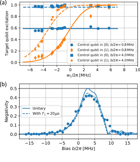
Figure 5: (a) Final population of the output qubit as a function of the weight $w_{1}=-J$ for two different bias values $b/2\pi$ of $0.8\,\mathrm{MHz}$ and $4.0\,\mathrm{MHz}$. As expected, when the input qubit is in the $|0\rangle$ state, the final output state does not depend on the weight, while for control state $|1\rangle$ it follows the nonlinear activation function. The solid and dashed lines are derived from numerical simulations with no fit parameters. (b) Negativity of the final two-qubits state after preparing the input qubit in an equal superposition state and the output qubit in its ground state and applying the perceptron gate with a weight $w_{1}/2\pi=-5.2\,\mathrm{MHz}$. Negativity of a two-qubit state can range between $0$ for a separable state to $1/2$ for a maximally entangled state. Lines show the simulated negativity for perfect unitary dynamics (solid) and when including relaxation of the qubits with decay times of $T_{1}=20\,\mathrm{\mu s}$ (dashed).

We further characterize the perceptron gate with quantum process tomography Mohseni et al. (2008) and verify several important aspect of the implemented process with the extracted process matrices: It is expected to act as a controlled gate – that is, if the input qubit is prepared in one of the basis states $|0\rangle$, $|1\rangle$, the gate should leave it in this state, independently of the output qubit’s initial state. We calculate the average fidelity with which the process $\mathcal{M}$ satisfies this condition, i.e.

$$\overline{\mathcal{F}}=\frac{1}{2}\sum_{i\in\{0,1\}}\Big{\langle}\mathrm{Tr}\big{(}|i\rangle\langle i|\otimes\mathbbm{1}\big{)}\mathcal{M}\big{[}|i\rangle\langle i|\otimes|\varphi\rangle\langle\varphi|\big{]}\Big{\rangle}_{\varphi},$$ (4)

where $\langle\cdot\rangle_{\varphi}$ denotes averaging over the initial state $|\varphi\rangle$ of the input qubit. This average is calculated from the process matrix of $\mathcal{M}$ by directly using Eq. (4) and the identity $\big{\langle}|\varphi\rangle\langle\varphi|\big{\rangle}_{\varphi}=\mathbbm{1}/2$. The obtained fidelity values are independent of the detuning $\Delta$ and lie between 0.95 and 0.97, indicating that the implemented operation is to a good approximation a controlled gate. We also evaluate the purity of the final state averaged over the initially prepared state and obtain a value around 0.78 (for a $1.7\,\mu\mathrm{s}$ long pulse), independent of the qubit-drive detuning. This confirms that the gate is mostly a unitary process, limited slightly by qubit decoherence. The average purity value is consistent with typical observed qubit dephasing times which vary in our experiment between $10~{}\mu\rm{s}$ and $20~{}\mu\rm{s}$.

Finally, to show the entangling property of the perceptron gate, we prepare the input qubit in an equal superposition state and the output qubit in its ground state. We then apply the perceptron gate, extract the density matrix of the final two-qubit state and calculate its negativity Vidal and Werner (2002), which reaches nearly the maximum value of $1/2$ for bias values at which the activation functions for the two computational states of the input qubit are well separated (Fig. 5(b)). In the limit of large weight, the ideal operation at the mid-point between the activation function slopes would become equivalent (up to local phases) to a controlled NOT gate, preparing a Bell state and reaching maximum negativity.

Figure 6: (a) A circuit that implements the equivalent of the perceptron gate with a single input and a single output qubit. A controlled-$V$ operation needs to be applied for each possible string of the inputs, in this case $x_{\text{in}}\in\{0,1\}$. (b) The circuit can be simplified by applying one of the multi-qubit controlled operations as a single-qubit gate and adjusting the following operations. Here, $W(x=1)=V(x=1)\cdot V(x=0)^{\dagger}$. (c) The controlled-$W$ gate is further decomposed into at most two CNOT gates and three single qubit gates $A$, $B$ and $C$.

III Equivalent circuit and
scaling complexity

For a general, multi-qubit input register the perceptron’s action in Eq. (1) can be considered as a generalized multi-qubit conditional gate: A separate operation $V(x)$ is applied for each of the basis states $\ket{x}\equiv\ket{x_{1}x_{2}\ldots x_{N}}$ of the $N$ input qubits. This is in contrast to a single multi-qubit controlled operation, that applies the operation $V$ to a output qubit only if all input qubits are in the state $\ket{1}$. Thus, to implement the perceptron gate requires a multi-qubit controlled gate for each input basis state, in total $2^{N}$ operations. This can be reduced to $2^{N}-1$ by implementing the $V(x)$ of one of the input strings as a single qubit gate and adjusting all multi-qubit controlled operations accordingly. For small $N\lesssim 10$, a multi-qubit controlled gate can be decomposed into $2^{N+1}-2$ two-qubit gates Barenco et al. (1995), which gives us a total gate count for the equivalent circuit of $N_{g}=(2^{N}-1)(2^{N+1}-2)$, approaching $\sim 2^{2N+1}$ for large number of input qubits.

More specifically, the single-input perceptron implemented in this paper can be decomposed into single qubit gates and two CNOT gates (Fig. 6).The fidelity and total duration of a sequence is typically limited by the number of two-qubit gates in transmon-based architectures. Hence, when ignoring single qubit gates, the sequence equivalent to the perceptron gate would be implemented in a gate time of $\sim 120~{}\rm{ns}$ and with an estimated fidelity of $\sim 99.4\%$. Here, we have assumed state of the art CNOT/CZ gates with fidelities of up to $99.7\%$ Kjaergaard et al. (2020a, b) and gate times of $60\rm{ns}$. The advantage of the adiabatic protocol, with approximately constant time, over the equivalent unitary circuit becomes apparent as the number of input qubits is increased, as discussed in Appendix A. For example, when decomposing the perceptron gate with two input qubits the best scenario estimate suggests a fidelity of $\sim 94.7\%$ with a gate time of $\sim 1.1~{}\mu\textrm{s}$.

IV Discussion and Outlook

By realizing the adiabatic perceptron dynamics that activates the output qubit depending on the state of connected input qubits directly in hardware, we have demonstrated the basic building block of a quantum feed-forward neural network. In this co-design approach, we show that by changing the length of the perceptron adiabatic qubit pulse the shape of the activation function can be modified, whereas the ZZ shift mediated by a tunable coupler and the adiabatic drive final frequency can be tuned to modify the weights and bias, which allows for training of the neural network.

As an extension of the demonstrated single-digit input scenario, an efficient implementation of a multi-input quantum perceptron can be realized by coupling multiple input qubits, each with its own tunable coupler, to a single output qubit. Its cumulative frequency shift would be of the form shown in Eq. (3) Nigg and Girvin (2013). It is noteworthy that the adiabatic gate presented here leads to complex multi-qubit operations with two-body interactions only and with a gate time that is independent of the number of inputs. In contrast, the time to run the equivalent circuit scales exponentially in the number of qubits, with significant advantage of the co-designed perceptron expected already for the three-qubit input case. While the quantum perceptron we co-design exponentially reduces the number of required conventional gates, all-to-all connectivity between the qubits of adjacent layers is desired to fully benefit from this advantage. Limitations imposed by the number of couplers that can be physically attached to a single qubit or compromises in the connectivity between layers may reduce this advantage. Therefore, multi-qubit couplers Mezzacapo et al. (2014); Chancellor et al. (2016); Paik et al. (2016); Sameti et al. (2017) may become increasingly useful, as will be architectures that combine the presented adiabatic implementation of a perceptron with standard digital gate sequences.

To ensure proper trainability of the network, the range of achievable weigths and biases should allow to probe the activation function at both limits $f(x)\approx 1$ and $f(x)\approx 0$. For our implementation, the possible range of ZZ shifts should be comparable to the charateristic width of the adiabatic curve, that is in turn limited by the ability to follow the eigenstates adiabatically given by the speed of the gate. Therefore, to reduce the perceptron gate time one could envisage either non-adiabatic versions of the perceptron Ban et al. (2021), or an extended range of achievable ZZ coupling by AC Noguchi et al. (2020); Ganzhorn et al. (2019) or DC Xu et al. (2021) pulses on the tunable coupler.

While we have demonstrated the entangling power of the perceptron gate, evaluating quantum advantage in larger networks is subject to forthcoming investigations. For instance, it will be important to understand how decoherence will affect the result and what role the entanglement between the input and output layer plays, in particular if the input layer is in a superposition state. Partially tracing out input and hidden layers and recycling qubits might allow for larger networks and protect the results from decoherence of earlier layers. Moreover, an investigation of the effects of higher connectivity on the expressivity of the nextwork will be required.

Finally, neural networks based on adiabatic perceptron gates may also have applications not directly related to machine learning. As an example, it is plausible that their quantum counterparts could serve well to parametrize unitaries in variational quantum algorithms Farhi et al. (2014); Peruzzo et al. (2014); Kandala et al. (2017), similar to the efficient approximation capability found in classical neural networks.

V Acknowledgments

We thank Stephan Paredes, Andreas Fuhrer, Matthias Mergenthaler, Peter Müller and Clemens Müller for insightful discussions and the quantum team at IBM T. J. Watson Research Center, Yorktown Heights for the provision of qubit devices. We thank R. Heller and H. Steinauer for technical support. Fabrication of samples was financially supported by the ARO under contract W911NF-14-1-0124, F.R. and M. W. acknowledge funding by the European Commission Marie Curie ETN project QuSCo (Grant Nr. 765267), and M. P., S. W. and G. S. by the European FET-OPEN project Quromorphic (Grant Nr. 828826).

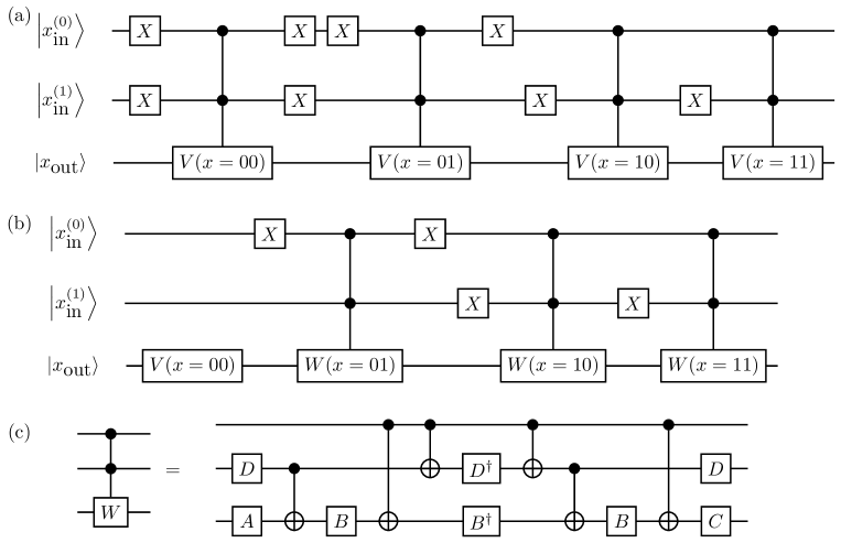
Figure 7: (a) Decomposition of the perceptron gate with two inputs and a single output qubit into controlled-controlled-$V$ operations and single-qubit operations $X$. (b) Improved circuit decomposition: one of the controlled-controlled operations, $V(00)$, is applied as a single-qubit gate with a simple adjustment $V(x)\rightarrow W(x)=V(x)V(00)^{\dagger}$ for the other controlled-controlled operations. (c) Decomposition of a controlled-controlled-$W$ gate in terms of 6 CNOT gates and 8 single-qubit gates.

Appendix A Equivalent unitary

The equivalent unitary matrix for the adiabatic perceptron can be expressed in terms of standard gates such a two-qubit controlled NOT and single qubit gates. However, the depth of the equivalent circuit grows exponentially with the number of input qubits.

The action of the perceptron in Eq. (1) can be thought of as a generalized multi-conditional gate. Whereas a ‘conventional’ N-controlled-$V$ operation applies the gate $V$ to a output qubit only if the control qubit (or qubits, for a multi-qubit controlled gate) is in the $\ket{1}$ state, in the perceptron gate for every computational basis state $\ket{x}\equiv\ket{x_{1}x_{2}\ldots x_{N}}$ with $x_{i}\in\{0,1\}$ of the control qubits a different gate $V(x)$ is applied to the output qubit. The matrix representation for such a controlled-gate has a block-diagonal structure

$$U=\begin{pmatrix}V(x=0\dots 0)&&&\\ &V(x=0\dots 1)&&\\ &&\ddots&\\ &&&V(x=1\dots 1)\end{pmatrix}$$

with each block $V(x)$ corresponding to a particular input string $x$. Thus, the perceptron gate can be expressed in terms of multi-qubit controlled unitaries as illustrated for a single input qubit in Fig. 6(a) and for two input qubits in Fig. 7(a). However, the number of multi-qubit controlled unitaries can be decreased by one by applying one the $V(x)$ gates as a single qubit gates, e.g. the unitary $V(x=0\dots 0)$ conditioned on all inputs being in the ground state, and adjusting all other multi-qubit controlled gates so as to account for the extra operation, in this example $V(x)\rightarrow W(x)=V(x)V(0\dots 0)^{\dagger}$. See Fig. 6(b) and Fig. 7(b) for one- and two-input qubits examples.

When acting on an output qubit initialized in the $\ket{0}$ state, the perceptron gate corresponds to the map

$$\ket{x}\otimes\ket{0}\rightarrow\ket{x}\otimes\left(\sqrt{1-|c(x)|^{2}}\ket{0}+c(x)\ket{1}\right).$$ (5)

By imposing unitarity, we can infer the action of the perceptron gate on a output qubit in the $\ket{1}$ state, and the controlled-$V(x)$ gate with

$$V(x)=\begin{pmatrix}\sqrt{1-|c(x)|^{2}}&c^{*}(x)\\ -c(x)&\sqrt{1-|c(x)|^{2}}.\end{pmatrix}.$$ (6)

For real $c(x)$, we can write $c(x)=\sin\theta_{x}/2$ and $\sqrt{1-c^{2}(x)}=\cos\theta_{x}/2$ and express $V(x)$ as

$$V(x)=\begin{pmatrix}\cos\theta_{x}/2&\sin\theta_{x}/2\\ -\sin\theta_{x}/2&\cos\theta_{x}/2\end{pmatrix}=R_{y}(\theta_{x}).$$ (7)

That is to say, the perceptron reduces to a sequence of rotations around the $X,Y$ and $Z$ axes. The number of multi-qubit controlled rotations in this decomposition is equal to the number of possible input bitstrings, which scales exponentially with the number of input qubits. As discussed in the main text, this may lead to a potential advantage of this protocol over more standard paramaterized gates.

Moreover, near-term quantum computers cannot generally implement multi-qubit controlled gates at once, but rather must decompose them into a series of one- and two-qubit gates as shown in  Figs. 6(c) and 7(c) by using CNOT gates as the primitive two-qubit operation.

In the main text, we use gate times and fidelities quoted for CZ instead of CNOT gates, being $F=99.7\%$ and $\tau=60~{}\rm{ns}$ as these are currently better for state-of-the-art transmon qubit architectures and since a CZ can easily be transformed to a CNOT via single qubit gates.

With these decompositions, and assuming that the two-qubit gates are the dominant source of error, we obtain estimates for the equivalent fidelities and gate times quoted in the main text: for the two-qubit (single-input, single-output) gate, 2 CNOTs are needed, leading to a fidelity of $\sim 98\%$ and a gate time of $\sim 240~{}\rm{ns}$; for the three-qubit (two inputs, one output) gate 18 CNOTs are needed, leading to a fidelity of $\sim 91\%$ and a gate time of $\sim 1.1~{}\mu\textrm{s}$. Gate time and fidelity estimates for more inputs are summarised in Table 1.

$N$	1	2	3	4
$N_{g}$	2	18	98	450
$t$ ($\mu$s)	0.12	1.1	5.9	27
$\mathcal{F}$	0.994	0.95	0.75	0.26

Table 1: Number of CNOT gates $N_{g}$ required for a circuit equivalent to the adiabatic ramp protocol with $N$ input qubits, along with estimates for the total circuit time $t$ and the circuit fidelity $\mathcal{F}$.

Appendix B Hamiltonian and Perturbation theory

The Hamiltonian describing the system is

$$H/\hbar=\sum_{i=1,2,c} \omega_{i}a_{i}^{\dagger}a_{i}+\frac{\alpha_{i}}{2}a_{i}^{\dagger}a_{i}^{\dagger}a_{i}a_{i}$$ (8)

$$+\sum_{i=1,2}g_{ic}(a_{i}-a_{i}^{\dagger})(a_{c}-a_{c}^{\dagger})$$

where $a_{i}^{\dagger}$ ($a_{i}$) are creation (annihilation) operators, $\omega_{i}$ are the frequencies and $\alpha_{i}$ are the anharmonicities of qubits ($i=1,2$) and coupler ($i=c$), and $g_{ic}$ are their respective couplings.

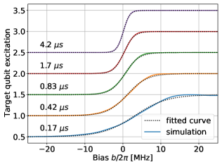
Figure 8: Comparison for different gate times of the simulated populations, solid line, and fits to the analytical (Eq. 11) from Hioe (1984). The analytical form well describes the simulated results, with small deviations for short gate times.

The anharmonicities $\alpha_{i}$ are defined as the difference $\omega_{12}-\omega_{01}$ between the $0\leftrightarrow 1$ and $1\leftrightarrow 2$ transition frequencies; values for the measured parameters can be found in Ganzhorn et al. (2019).

Using fourth-order perturbation theory, we can approximate the ZZ coupling strength $J$ as

$$J=2g_{1c}^{2}g_{2c}^{2}\frac{\alpha_{1}\alpha_{2}(\Delta_{1}+\Delta_{2})^{2}+\alpha_{2}\alpha_{c}\Delta_{1}^{2}+\alpha_{1}\Delta_{1}^{2}(\Delta_{1}+\Delta_{2})+\alpha_{2}\Delta_{2}^{2}(\Delta_{1}+\Delta_{2})+\alpha_{c}(\Delta_{1}+\Delta_{2})(\Delta_{1}-\Delta_{2})^{2}}{\Delta_{1}^{2}\Delta_{2}^{2}(\Delta_{1}+\Delta_{2}+\alpha_{c})(\Delta_{2}-\Delta_{1}-\alpha_{2})(\Delta_{1}-\Delta_{2}-\alpha_{1}),}$$ (9)

where $\Delta_{1,2}=\omega_{c}-\omega_{1,2}$ are the detunings of the coupler from the two qubits.

Appendix C Analytic solution for chirped pulses

The driven two level system, although ubiquitous, has proven to notoriously difficult to solve analytically. The most well known analytical solution is the Landau-Zener linear ramp Landau (1932); Zener (1932). Soon after another exact solution was found for a hyperbolic secant pulse Rosen and Zener (1932) and was later extensively used McCall and Hahn (1969), analysed and extended Hioe (1984). The hyperbolic secant pulse is chirped to have a detuning $\omega_{\mathrm{p}}(t)$ and modulated in amplitude $\Omega(t)$ according to:

$$\omega_{\mathrm{p}}(t) =\omega_{\mathrm{i}}+(\omega_{\mathrm{f}}-\omega_{\mathrm{i}})\tanh^{2}(\pi t/T),$$ (10)

$$\Omega(t) =\Omega_{0}\sech(\pi t/T).$$

Assuming that the pulse begins at time $t=-\infty$ and ends at time $t=+\infty$ one can find an analytical expression for the population transfer at the end of the pulse. This is given as

$$P_{1}(+\infty)=\sech\left[(\omega_{i}+\Delta_{f})T/2\right]\sech\left[(\omega_{i}-\Delta_{f})T/2\right]\left[\sin^{2}(\sqrt{\Omega_{0}^{2}+\Delta_{f}^{2}}T/2)+\sinh^{2}(\Delta_{f}T/2)\right]$$ (11)

The chirped pulses in our experiment can be obtained from the ones described above by applying the time transformation

$$t\rightarrow\mathrm{artanh}(-\cos(\pi*t^{\prime}/T))*T$$

and indeed define the same trajectory in the detuning versus amplitude plane. When we compare the analytical solution described above with the simulation results we find agreement in the curve behaviour (Fig. 8). Differences in steepness of the curves are due to the time transformation between the two cases. Nonetheless the underlying sigmoid behaviour remains, and the curves can be precisely matched by allowing for the fitting parameter $T$ and a further detuning of the whole curve $\delta$, given by $\omega_{i}\rightarrow\omega_{i}+\delta$.

References

- Torrontegui and García-Ripoll (2019) Erik Torrontegui and Juan José García-Ripoll, “Unitary quantum perceptron as efficient universal approximator,” Europhysics Letters 125, 30004 (2019).
- Biamonte et al. (2017) Jacob Biamonte, Peter Wittek, Nicola Pancotti, Patrick Rebentrost, Nathan Wiebe, and Seth Lloyd, “Quantum machine learning,” Nature 549, 195–202 (2017).
- Rocchetto et al. (2018) Andrea Rocchetto, Edward Grant, Sergii Strelchuk, Giuseppe Carleo, and Simone Severini, “Learning hard quantum distributions with variational autoencoders,” npj Quantum Information 4, 1–7 (2018).
- Das Sarma et al. (2019) Sankar Das Sarma, Dong-Ling Deng, and Lu-Ming Duan, “Machine learning meets quantum physics,” Physics Today 72, 48–54 (2019).
- Zoufal et al. (2019) Christa Zoufal, Aurélien Lucchi, and Stefan Woerner, “Quantum generative adversarial networks for learning and loading random distributions,” npj Quantum Information 5, 1–9 (2019).
- Melko et al. (2019) Roger G Melko, Giuseppe Carleo, Juan Carrasquilla, and J Ignacio Cirac, “Restricted boltzmann machines in quantum physics,” Nature Physics 15, 887–892 (2019).
- Abbas et al. (2021) Amira Abbas, David Sutter, Christa Zoufal, Aurélien Lucchi, Alessio Figalli, and Stefan Woerner, “The power of quantum neural networks,” Nature Computational Science 1, 403–409 (2021).
- Havlíček et al. (2019) Vojtěch Havlíček, Antonio D Córcoles, Kristan Temme, Aram W Harrow, Abhinav Kandala, Jerry M Chow, and Jay M Gambetta, “Supervised learning with quantum-enhanced feature spaces,” Nature 567, 209–212 (2019).
- Glick et al. (2021) Jennifer R Glick, Tanvi P Gujarati, Antonio D Corcoles, Youngseok Kim, Abhinav Kandala, Jay M Gambetta, and Kristan Temme, “Covariant quantum kernels for data with group structure,” arXiv:2105.03406 (2021).
- Harrow et al. (2009) Aram W. Harrow, Avinatan Hassidim, and Seth Lloyd, “Quantum algorithm for linear systems of equations,” Phys. Rev. Lett. 103, 150502 (2009).
- Farhi et al. (2014) Edward Farhi, Jeffrey Goldstone, and Sam Gutmann, “A quantum approximate optimization algorithm,” arXiv:1411.4028 (2014).
- Peruzzo et al. (2014) Alberto Peruzzo, Jarrod McClean, Peter Shadbolt, Man-Hong Yung, Xiao-Qi Zhou, Peter J Love, Alán Aspuru-Guzik, and Jeremy L O’Brien, “A variational eigenvalue solver on a photonic quantum processor,” Nature Communications 5, 4213 (2014).
- Moll et al. (2018) Nikolaj Moll, Panagiotis Barkoutsos, Lev S Bishop, Jerry M Chow, Andrew Cross, Daniel J Egger, Stefan Filipp, Andreas Fuhrer, Jay M Gambetta, Marc Ganzhorn, et al., “Quantum optimization using variational algorithms on near-term quantum devices,” Quantum Science and Technology 3, 030503 (2018).
- Kandala et al. (2017) Abhinav Kandala, Antonio Mezzacapo, Kristan Temme, Maika Takita, Markus Brink, Jerry M Chow, and Jay M Gambetta, “Hardware-efficient variational quantum eigensolver for small molecules and quantum magnets,” Nature 549, 242–246 (2017).
- Liu et al. (2021) Yunchao Liu, Srinivasan Arunachalam, and Kristan Temme, “A rigorous and robust quantum speed-up in supervised machine learning,” Nature Physics , 1–5 (2021).
- Pérez-Salinas et al. (2021) Adrián Pérez-Salinas, David López-Núñez, Artur García-Sáez, P. Forn-Díaz, and José I. Latorre, “One qubit as a universal approximant,” Phys. Rev. A 104, 012405 (2021).
- Behrman et al. (2000) E.C. Behrman, L.R. Nash, J.E. Steck, V.G. Chandrashekar, and S.R. Skinner, “Simulations of quantum neural networks,” Information Sciences 128, 257–269 (2000).
- Schuld et al. (2014) Maria Schuld, Ilya Sinayskiy, and Francesco Petruccione, “The quest for a quantum neural network,” Quantum Information Processing 13, 2567–2586 (2014).
- Cao et al. (2017) Yudong Cao, Gian Giacomo Guerreschi, and Alán Aspuru-Guzik, “Quantum neuron: an elementary building block for machine learning on quantum computers,” arXiv:1711.11240 (2017).
- Fredkin and Toffoli (1982) Edward Fredkin and Tommaso Toffoli, “Conservative logic,” International Journal of theoretical physics 21, 219–253 (1982).
- Yan et al. (2020) Shilu Yan, Hongsheng Qi, and Wei Cui, “Nonlinear quantum neuron: A fundamental building block for quantum neural networks,” Phys. Rev. A 102, 052421 (2020).
- Koch et al. (2007) Jens Koch, Terri M. Yu, Jay Gambetta, A. A. Houck, D. I. Schuster, J. Majer, Alexandre Blais, M. H. Devoret, S. M. Girvin, and R. J. Schoelkopf, “Charge-insensitive qubit design derived from the Cooper pair box,” Physical Review A 76, 042319 (2007).
- McKay et al. (2016) David C. McKay, Stefan Filipp, Antonio Mezzacapo, Easwar Magesan, Jerry M. Chow, and Jay M. Gambetta, “Universal gate for fixed-frequency qubits via a tunable bus,” Physical Review Applied 6, 064007 (2016).
- Li et al. (2020) X. Li, T. Cai, H. Yan, Z. Wang, X. Pan, Y. Ma, W. Cai, J. Han, Z. Hua, X. Han, Y. Wu, H. Zhang, H. Wang, Yipu Song, Luming Duan, and Luyan Sun, “Tunable coupler for realizing a controlled-phase gate with dynamically decoupled regime in a superconducting circuit,” Phys. Rev. Applied 14, 024070 (2020).
- Roth et al. (2019) Marco Roth, Nikolaj Moll, Gian Salis, Marc Ganzhorn, Daniel J. Egger, Stefan Filipp, and Sebastian Schmidt, “Adiabatic quantum simulations with driven superconducting qubits,” Phys. Rev. A 99, 022323 (2019).
- Salis et al. (2020) Gian Salis, Nikolaj Moll, Marco Roth, Marc Ganzhorn, and Stefan Filipp, “Time-resolved tomography of a driven adiabatic quantum simulation,” Phys. Rev. A 102, 062611 (2020).
- Hioe (1984) F. T. Hioe, “Solution of bloch equations involving amplitude and frequency modulations,” Phys. Rev. A 30, 2100–2103 (1984).
- Baum et al. (1985) J. Baum, R. Tycko, and A. Pines, “Broadband and adiabatic inversion of a two-level system by phase-modulated pulses,” Phys. Rev. A 32, 3435–3447 (1985).
- Mohseni et al. (2008) M. Mohseni, A. T. Rezakhani, and D. A. Lidar, “Quantum-process tomography: Resource analysis of different strategies,” Phys. Rev. A 77, 032322 (2008).
- Vidal and Werner (2002) G. Vidal and R. F. Werner, “Computable measure of entanglement,” Phys. Rev. A 65, 032314 (2002).
- Barenco et al. (1995) Adriano Barenco, Charles H. Bennett, Richard Cleve, David P. DiVincenzo, Norman Margolus, Peter Shor, Tycho Sleator, John A. Smolin, and Harald Weinfurter, “Elementary gates for quantum computation,” Phys. Rev. A 52, 3457–3467 (1995).
- Kjaergaard et al. (2020a) Morten Kjaergaard, Mollie E Schwartz, Ami Greene, Gabriel O Samach, Andreas Bengtsson, Michael O’Keeffe, Christopher M McNally, Jochen Braumüller, David K Kim, Philip Krantz, et al., “Programming a quantum computer with quantum instructions,” arXiv:2001.08838 (2020a).
- Kjaergaard et al. (2020b) Morten Kjaergaard, Mollie E. Schwartz, Jochen Braumüller, Philip Krantz, Joel I.-J. Wang, Simon Gustavsson, and William D. Oliver, “Superconducting qubits: Current state of play,” Annual Review of Condensed Matter Physics 11, 369–395 (2020b).
- Nigg and Girvin (2013) Simon E. Nigg and S. M. Girvin, “Stabilizer quantum error correction toolbox for superconducting qubits,” Phys. Rev. Lett. 110, 243604 (2013).
- Mezzacapo et al. (2014) Antonio Mezzacapo, U Las Heras, JS Pedernales, L DiCarlo, E Solano, and L Lamata, “Digital quantum rabi and dicke models in superconducting circuits,” Scientific Reports 4, 1–4 (2014).
- Chancellor et al. (2016) Nicholas Chancellor, Aleks Kissinger, Joschka Roffe, Stefan Zohren, and Dominic Horsman, “Graphical structures for design and verification of quantum error correction,” arXiv:1611.08012 (2016).
- Paik et al. (2016) Hanhee Paik, A. Mezzacapo, Martin Sandberg, D. T. McClure, B. Abdo, A. D. Córcoles, O. Dial, D. F. Bogorin, B. L. T. Plourde, M. Steffen, A. W. Cross, J. M. Gambetta, and Jerry M. Chow, “Experimental demonstration of a resonator-induced phase gate in a multiqubit circuit-qed system,” Phys. Rev. Lett. 117, 250502 (2016).
- Sameti et al. (2017) Mahdi Sameti, Anton Potočnik, Dan E. Browne, Andreas Wallraff, and Michael J. Hartmann, “Superconducting quantum simulator for topological order and the toric code,” Phys. Rev. A 95, 042330 (2017).
- Ban et al. (2021) Yue Ban, Xi Chen, E. Torrontegui, E. Solano, and J. Casanova, “Speeding up quantum perceptron via shortcuts to adiabaticity,” Scientific Reports 11, 5783 (2021).
- Noguchi et al. (2020) Atsushi Noguchi, Alto Osada, Shumpei Masuda, Shingo Kono, Kentaro Heya, Samuel Piotr Wolski, Hiroki Takahashi, Takanori Sugiyama, Dany Lachance-Quirion, and Yasunobu Nakamura, “Fast parametric two-qubit gates with suppressed residual interaction using the second-order nonlinearity of a cubic transmon,” Phys. Rev. A 102, 062408 (2020).
- Ganzhorn et al. (2019) Marc Ganzhorn, Daniel Josef Egger, Stefan Filipp, Gian R von Salis, and Nikolaj Moll, “Cross-talk compensation in quantum processing devices,” (2019), US Patent 10,452,991.
- Xu et al. (2021) Huikai Xu, Weiyang Liu, Zhiyuan Li, Jiaxiu Han, Jingning Zhang, Kehuan Linghu, Yongchao Li, Mo Chen, Zhen Yang, Junhua Wang, et al., “Realization of adiabatic and diabatic CZ gates in superconducting qubits coupled with a tunable coupler,” Chinese Physics B 30, 044212 (2021).
- Landau (1932) Lev Davidovich Landau, “Zur theorie der energieubertragung ii,” Z. Sowjetunion 2, 46–51 (1932).
- Zener (1932) Clarence Zener, “Non-adiabatic crossing of energy levels,” Proceedings of the Royal Society of London. Series A, Containing Papers of a Mathematical and Physical Character 137, 696–702 (1932).
- Rosen and Zener (1932) Nathan Rosen and Clarence Zener, “Double stern-gerlach experiment and related collision phenomena,” Physical Review 40, 502 (1932).
- McCall and Hahn (1969) Samuel Leverte McCall and Erwin L Hahn, “Self-induced transparency,” Physical Review 183, 457 (1969).