An MAP Estimation for Between-Class Variance

Abstract

Probabilistic linear discriminant analysis (PLDA) has been widely used in open-set verification tasks, such as speaker verification. A potential issue of this model is that the training set often contains limited number of classes, which makes the estimation for the between-class variance unreliable. This unreliable estimation often leads to degraded generalization. In this paper, we present an MAP estimation for the between-class variance, by employing an Inverse-Wishart prior. A key problem is that with hierarchical models such as PLDA, the prior is placed on the variance of class means while the likelihood is based on class members, which makes the posterior inference intractable. We derive a simple MAP estimation for such a model, and test it in both PLDA scoring and length normalization. In both cases, the MAP-based estimation delivers interesting performance improvement.

1 Introduction

Probabilistic linear discriminant analysis (PLDA) [1, 2, 3] has been extensively used in open-set verification tasks, such as speaker verification [4, 5, 6]. It represents the data with a linear Gaussian model, where the between-class distribution is a Gaussian and the within-class distributions of individual classes are homogeneous Gaussians. The parameters of this model involve a linear transform matrix $\mathbf{M}$ and the between-class covariance of the data after the linear transform, and they can be estimated by maximum likelihood (ML) training. Once the model has been trained, it is possible to decide whether two samples are produced from the same class or from two different classes [1], and this decision is optimal in terms of minimum Bayes risk (MBR) [7].

A potential problem of PLDA is the unreliable estimation for the between-class covariance, denoted by $S_{B}$. In many applications, the number of classes in the training data is limited. Take speaker verification as an example, the largest open-source dataset VoxCeleb contains 7,000+ speakers. Considering the high dimensionality of the data (e.g., speaker vectors in speaker verification, whose dimension is 400-600), it is difficult to estimate a reasonable between-speaker covariance with maximum likelihood training.

To have an intuition, we take a simulation experiment by sampling $n$ samples from a Gaussian distribution and a Laplacian distribution, and then compute the ML-based variance estimation for each sampling. We plot the variance’s variance to show the reliability of the estimation. As shown in Fig. 1, when the number of samples $n$ is small, the variance’s variance is large, indicating that the estimation is highly unreliable. This conclusion is more clear with the Laplacian distribution, due to its heavy-tail property.

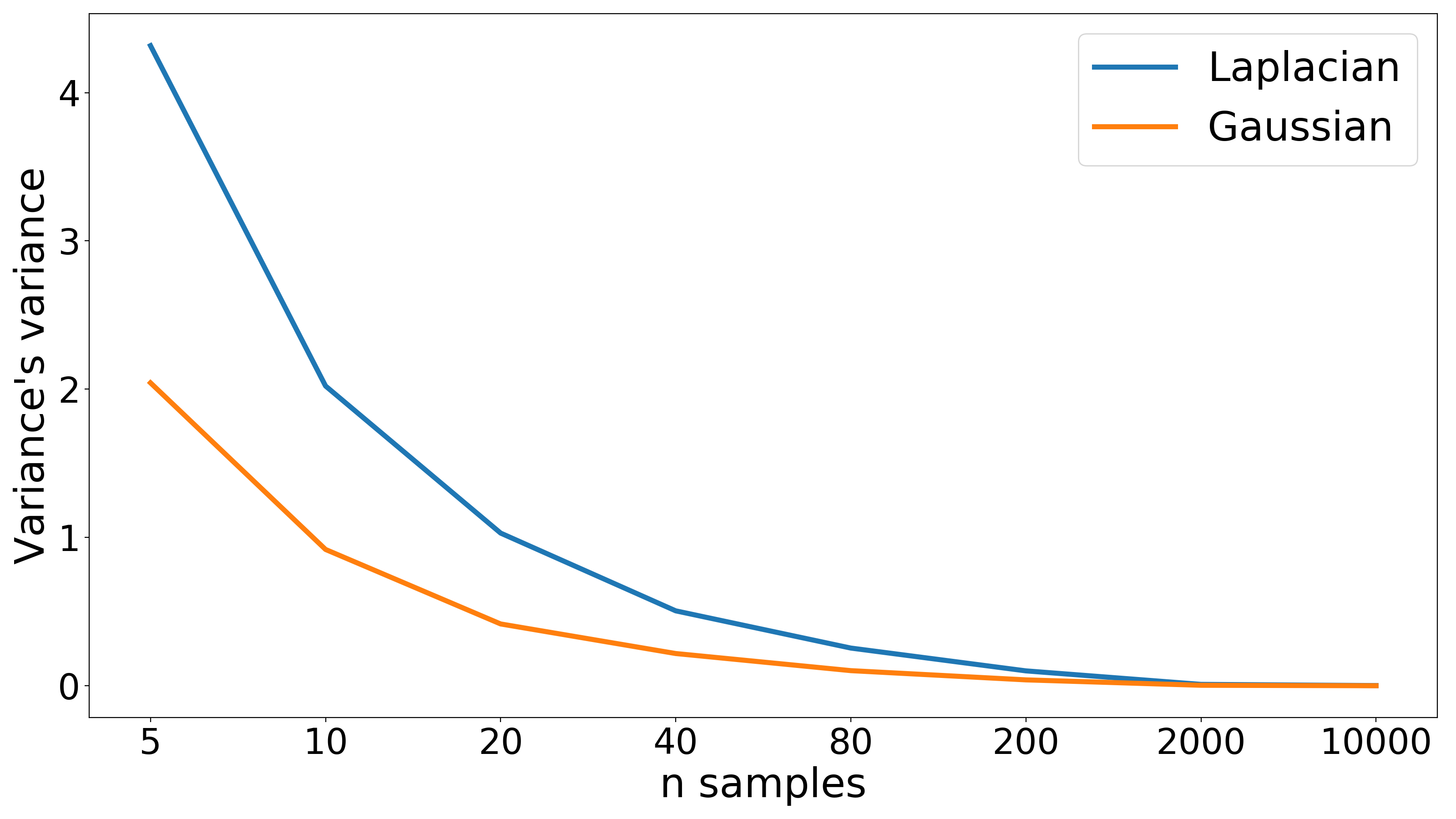
Figure 1: Variance’s variance of $n$ samples from Gaussian and Laplacian distributions. For each distribution, we firstly sample $n$ data points, and then compute their variance $\sigma$ (i.e., ML-based estimation for the underlying true variance). This process repeats 10,000 times and the variance of the 10,000 $\sigma$ values is computed. The x-axis is the number of samples $n$, and the y-axis is the value of variance’s variance. For simplicity, the data points are one-dimensional. For the sake of comparison, the true variances of two distributions are both set to 1.0.

For PLDA, the limited number of classes leads to the same unreliable estimation for the between-class covariance $S_{B}$. For speaker verification, the distribution of speaker vectors is known to be heavy-tailed [8], which makes the ML estimation for $S_{B}$ even more unreliable. Moreover, the dimensionality of speaker vectors is often as high as 400-600, which further exaggerates the problem.

In this paper, we propose a robust estimation for the between-class variance $S_{B}$, by placing an Inverse-Wishart prior on $S_{B}$ and then conduct maximum a posterior (MAP) estimation. At the first glance, the MAP estimation seems trivial if the prior and the associated conditional likelihood are given. However, for hierarchical probabilistic models such as PLDA, it is much more convolved. This is because the prior is placed on the covariance of the class means while the likelihood is based on the class members. This complication leads to intractable inference for $S_{B}$. We will prove that under some mild conditions, the MAP estimation can be reformulated to a simple linear interpolation of $S_{B}$ derived by the standard PLDA and a prior covariance.

2 Theory

2.1 Preliminary of PLDA

We consider the two-covariance form of the PLDA model [3], which assumes a linear Gaussian as follows, where $k$ indexes the class, and $i$ indexes samples of a particular class:

$$\boldsymbol{x}_{ki}=\boldsymbol{\mu}_{0}+\mathbf{M}\boldsymbol{\mu}_{k}+\boldsymbol{n}_{ki},$$ (1)

$$\boldsymbol{\mu}_{k}\sim\mathcal{N}(\mathbf{0},diag(\boldsymbol{\epsilon})),$$ (2)

$$\boldsymbol{n}_{ki}\sim\mathcal{N}(\mathbf{0},\mathbf{I}),$$ (3)

where we assume $\mathbf{M}$ is of full rank. By this assumption, the within-class covariance is the identity matrix $\mathbf{I}$, and the between-class covariance is computed as follows:

$$S_{B}=\mathbf{M}diag(\boldsymbol{\epsilon})\mathbf{M}^{T}.$$ (4)

The likelihood of the data of a particular class $k$ can be computed as follows:

$$p(\boldsymbol{x}_{1},\boldsymbol{x}_{2},...,\boldsymbol{x}_{n_{k}}) = \int p(\boldsymbol{x}_{1},...,\boldsymbol{x}_{n_{k}}|\boldsymbol{\mu}_{k})p(\boldsymbol{\mu}_{k}){\rm d}\boldsymbol{\mu}_{k}$$ (5)

$$= \int\prod_{i=1}^{n_{k}}p(\boldsymbol{x}_{i}|\boldsymbol{\mu}_{k})p(\boldsymbol{\mu}_{k}){\rm d}\boldsymbol{\mu}_{k}.$$

Since $p(\boldsymbol{x}_{i}|\boldsymbol{\mu}_{k})$ and $p(\boldsymbol{\mu}_{k})$ are both Gaussian, it is easy to show that $p(\boldsymbol{x}_{1},\boldsymbol{x}_{2},...,\boldsymbol{x}_{n_{k}})$ is Gaussian and can be computed efficiently. Collecting all the data of $K$ classes, the likelihood function can be computed as follows:

$$\mathcal{L}(\boldsymbol{\epsilon},\mathbf{M},\boldsymbol{\mu}_{0})=\prod_{k=1}^{K}p(\boldsymbol{x}^{k}_{1},...,\boldsymbol{x}^{k}_{n_{k}}),$$ (6)

where $\boldsymbol{\epsilon},\mathbf{M},\boldsymbol{\mu}_{0}$ are the parameters. Maximizing this function with respect to these parameters leads to a maximum likelihood (ML) training.

Once the model has been trained, it can be employed to perform verification tasks. According to the hypothesis test theory [9], the following likelihood ratio (LR) is optimal in terms of Bayes risk, when used to judge whether a test sample $\boldsymbol{x}$ belongs to the class represented by the enrollment samples $\{\boldsymbol{x}_{1},...,\boldsymbol{x}_{n}\}$:

$$\emph{LR}=\frac{p(\boldsymbol{x},\boldsymbol{x}_{1},...,\boldsymbol{x}_{n})}{p(\boldsymbol{x})p(\boldsymbol{x}_{1},...,\boldsymbol{x}_{n})}.$$ (7)

Thanks to the linear Gaussian form of the model, the LR score has a closed form and can be computed efficiently [1, 2].

2.2 MAP estimation for $S_{B}$

Suppose an Inverse-Wishart prior on $\boldsymbol{\epsilon}$ [10]:

$$p(\boldsymbol{\epsilon};\boldsymbol{\phi},\nu)=\frac{1}{Z}(\prod_{j=1}^{p}\epsilon_{j})^{-\frac{\nu+p+1}{2}}\exp\{-\frac{1}{2}\prod_{j=1}^{p}\phi_{j}\epsilon^{-1}_{j}\},$$ (8)

where $p$ is the dimension of the data and $Z$ is a normalization term. If there are $n$ observations following a Gaussian, it is easy to derive that the MAP estimation for $\boldsymbol{\epsilon}$ is given as follows [10]:

$$\boldsymbol{\epsilon}_{\emph{MAP}}=\frac{\boldsymbol{\phi}+n\boldsymbol{\epsilon}_{\emph{ML}}}{\nu+n+p+1},$$ (9)

where $\boldsymbol{\epsilon}_{\emph{ML}}$ denotes the ML estimation for $\boldsymbol{\epsilon}$ with $n$ observations.

If we place an Inverse-Wishart prior on $S_{B}$ of the PLDA model, the graphical representation is shown in Fig. 2. In this case, the interaction between $\bm{\epsilon}$ and the observation $\bm{x}$ is indirect, and there are no i.i.d. Gaussian samples can be used to estimate $\boldsymbol{\epsilon}_{\emph{MAP}}$ by (9). One possibility is to use the likelihood function (5) as the conditional probability, and derive the MAP estimation as follows:

$$\boldsymbol{\epsilon}_{\emph{MAP}}=\arg\max_{\boldsymbol{\epsilon}}p(\boldsymbol{\epsilon};\boldsymbol{\phi},\nu)\prod_{k}p(\boldsymbol{x}_{1},\boldsymbol{x}_{2},...,\boldsymbol{x}_{n_{k}}|\boldsymbol{\epsilon})$$ (10)

Figure 2: Graphical model of PLDA with an Inverse-Wishart prior on the between-class variance $\boldsymbol{\epsilon}$.

Since $\prod_{k}p(\boldsymbol{x}_{1},\boldsymbol{x}_{2},...,\boldsymbol{x}_{n_{k}}|\boldsymbol{\epsilon})$ involves an undetermined parameter $\mathbf{M}$ and needs to marginalize on $\boldsymbol{\mu}_{k}$, the inference for $\boldsymbol{\epsilon}_{\emph{MAP}}$ is intractable. Although a variational approach can be used [11], the iterative process leads to increased computational load. We will show that a simple MAP estimation can be derived by using $\pm{\epsilon}$ derived from the standard PLDA, under mild conditions.

Proposition 1.

If every class involves $n$ training samples, and PLDA has been well trained, the between-class covariance $\bm{\epsilon}$ can be written as $\bm{\epsilon}=\frac{\sum_{k}\bar{\bm{x}}^{\prime}_{k}}{K}-1/n$, where $\bar{\boldsymbol{x}}^{\prime}_{k}=\frac{1}{n}\sum_{i=1}^{n}\mathbf{M}^{-1}(\boldsymbol{x}_{ki}-\boldsymbol{\mu}_{0})$.

Proof.

Since the PLDA model has been well trained, $\bm{x}^{\prime}=\mathbf{M}^{-1}(\bm{x}-\bm{\mu}_{0})$ show a regulated distribution: the between-class variance is $diag(\bm{\epsilon})$, and the within-class variance is $\mathbf{I}$. Considering a particular class, the joint probability of the class members is a function of $\bm{\epsilon}$. Considering a particular dimension $j$, the probability is given by:

$$p(\bm{x}_{1},...,\bm{x}_{n};\epsilon_{j})$$ (11)

$$\propto \int\frac{1}{\epsilon_{j}^{1/2}}\exp\big{\{}-\frac{1}{2\epsilon_{j}}\mu^{2}\big{\}}\prod_{i}^{n}\exp\big{\{}-\frac{1}{2}(x^{\prime}_{ij}-\mu)^{2}\big{\}}\rm{d}\mu$$

$$= \frac{1}{\epsilon_{j}^{1/2}}\int\exp\big{\{}-\frac{1}{2\epsilon_{j}}\mu^{2}-\frac{1}{2}\sum_{i}(x^{\prime}_{ij}-\mu)^{2}\big{\}}\rm{d}\mu$$

$$= \frac{1}{\epsilon_{j}^{1/2}}\int\exp\big{\{}-\frac{(1+n\epsilon)}{2\epsilon_{j}}((\mu-\frac{\epsilon_{j}}{(1+n\epsilon_{j})}\sum_{i}x^{\prime}_{ij})^{2}$$

$$-\frac{\epsilon_{j}^{2}}{(1+n\epsilon_{j})^{2}}\sum_{i}(x^{\prime}_{ij})^{2})\big{\}}\rm{d}\mu$$

$$\propto \frac{1}{(1+n\epsilon_{j})^{1/2}}\exp\big{\{}\frac{n^{2}\epsilon_{j}}{2(1+n\epsilon_{j})}(\bar{x}^{\prime}_{j})^{2}\big{\}}$$

Considering all the classes:

$$\mathcal{L}(\epsilon_{j}) = \sum_{k=1}^{K}\ln p(x_{1}^{k},x_{2}^{k},...,x_{n}^{k};\epsilon_{j})$$

$$= -\frac{K}{2}\ln(n\epsilon_{j}+1)+\frac{n^{2}\epsilon_{j}}{2(1+n\epsilon_{j})}\sum_{k}(\bar{x}^{\prime}_{jk})^{2}+const$$

Take derivative of $\mathcal{L}(\epsilon_{j})$ with respect to $\epsilon_{j}$ and set it to 0:

$$\frac{\partial\mathcal{L}(\epsilon_{j})}{\partial\epsilon_{j}}=-\frac{K}{2}\frac{n}{n\epsilon_{j}+1}+\frac{1}{2}\sum_{k}(\bar{x}^{\prime}_{jk})^{2}\frac{n^{2}(1+n\epsilon_{j})-n^{3}\epsilon_{j}}{(1+n\epsilon_{j})^{2}}=0$$ (12)

A simple computation shows:

$$\epsilon_{j}=\frac{\sum_{k=1}^{K}(\bar{x}^{\prime}_{jk})^{2}}{K}-\frac{1}{n}$$ (13)

Since all the dimensions of $\bm{x}^{\prime}$ are independent, we have:

$$\bm{\epsilon}=\frac{\sum_{k=1}^{K}(\bar{\bm{x}}^{\prime}_{k})^{2}}{K}-\frac{1}{n}$$ (14)

∎

Obviously, if $n$ is large, the estimation for $\boldsymbol{\epsilon}$ approaches to:

$$\bm{\epsilon}\approx\frac{\sum_{k}(\bar{\bm{x}}^{\prime}_{k})^{2}}{K},$$ (15)

which can be interpreted as an ML estimation for the covariance of a Gaussian distribution represented by the $K$ virtual samples $\{\bar{\bm{x}}^{\prime}_{k}\}$.

Since $\boldsymbol{\epsilon}$ derived by PLDA is equivalent to $\boldsymbol{\epsilon}_{\emph{ML}}$ derived with the $K$ virtual samples $\{\bar{\bm{x}}^{\prime}_{k}\}$, we can use these virtual samples as the observations of the underlying Gaussian model, and derive the MAP estimation for the covariance of these samples:

$$\boldsymbol{\epsilon}_{\emph{MAP}}=\frac{\boldsymbol{\phi}+K\boldsymbol{\epsilon}}{\nu+K+p+1},$$ (16)

where $\boldsymbol{\epsilon}$ is obtained from the standard PLDA.

By defining appropriate $\boldsymbol{\phi}$ and $\nu$, the above equation can be reformulated as a simple linear interpolation:

$$\boldsymbol{\epsilon}_{\emph{MAP}}=\frac{\alpha\boldsymbol{\epsilon}_{0}+K\boldsymbol{\epsilon}}{\alpha+K},$$ (17)

where $\boldsymbol{\epsilon}_{0}$ can be interpreted as a prior covariance, and $\alpha$ is a hyper-parameter that represents the number of virtual samples associated with $\boldsymbol{\epsilon}_{0}$. We therefore derived a simple form of MAP estimation for the between-class variance with PLDA.

We highlight that although the final result (17) looks simple, it should not be regarded as trivial. In fact, to derive such a result, we have assumed that all the classes involve the same number of samples. This is even not true in most practical usage, demonstrating that (17) is not as straightforward as the first glance.

2.3 Applied to length normalization

The MAP-estimated $\bm{\epsilon}$ (and hence $S_{B}$) can be used directly in PLDA scoring, which we will call PLDA/MAP. Moreover, the more robust $S_{B}$ can be used to improve length normalization (LN) as well. LN is a simple and effective trick that has been widely used in speaker verification [12]. The key idea is that for a high-dimensional Gaussian distribution, most of the samples should concentrate on an eclipse surface defined by the covariance. Suppose the distribution has been aligned to the axes, the eclipse surface will be as follows:

$$\sum_{j}\frac{x_{j}^{2}}{\lambda_{j}}=p$$ (18)

where $\lambda_{j}$ is the variance of the $j$-th dimension. In the PLDA model, this variance consists of the between-class variance $\epsilon_{j}$ and the within-class variance $\sigma=1$, i.e., $\lambda_{j}=\epsilon_{j}+1$. LN scales the speaker vectors to this surface if they are not, with the scale factor computed by:

$$r=\frac{\sqrt{p}}{\sqrt{\sum_{j}\frac{x_{j}^{2}}{\epsilon_{j}+1}}}.$$ (19)

It has been shown that this scaling can greatly improve the Gaussianality of the speaker vectors, hence making them more suitable for PLDA modeling.

Here we encounter the same problem as in PLDA scoring: if $\boldsymbol{\epsilon}$ is not well estimated, the scaling will be incorrect. In particular for speaker vectors aligned to the directions corresponding to a large $\epsilon_{j}$, the scaling tends to be aggressive. The MAP-based estimation for $\boldsymbol{\epsilon}$ discounts large variance and thus is expected to alleviate this problem. For that purpose, we simply use $\boldsymbol{\epsilon}_{\emph{MAP}}$ to compute the scale factor $r$. We will call the revised length normalization as LN/MAP.

3 Related work

Brummer et al. [13] presented the initial idea of Bayes PLDA, with the aim to overcome the shortage associated with the point estimation for the parameters in the conventional ML-based PLDA model.

Villalba et al. [11] employed a Bayes approach to improve speaker verification with i-vectors [14]. This approach was further extended to deal with domain adaptation, where the PLDA parameters obtained in one domain were used as the prior when training PLDA in a new domain [15, 16]. Although theoretically interesting, it relies variational inference in both training and test, which is not very friendly and so is rarely used.

The Inverse-Wishart distribution was generally used as the prior for distance/correlation matrix. For example, Fang et al. [17] employed this prior to regularize the metric learning with an i-vector system. Ito et al. [16] employed this prior to adapt the covariance in the GMM-UBM architecture for speaker verification.

4 Experiments

We evaluate the proposed approach by a speaker verification task, following the deep speaker embedding framework [18, 19, 20]. Given a speech segment, a speaker vector is produced by a deep neural network which consists of frame-level feature extractor and utterance-level pooling. In this paper, we employ the x-vector model [21] to produce the speaker vectors. This model is trained using the Kaldi toolkit [22], following the SITW recipe . The dimensionality of the x-vectors was set to $512$. Once the speaker vectors are obtained, a PLDA model with LDA dimension reduction is trained and employed to score the test trials. Note that our research goal here is to demonstrate the MAP-based estimation for $S_{B}$ rather than present a SOTA speaker verification system. For this purpose, using a public recipe in Kaldi is a reasonable choice. Readers can refer to [23, 24] for SOTA performance on the same task.

Table 1: EER(%) results with different settings of PLDA and LN

	No.	Model	SITW.Dev	SITW.Eval	HI-MIA.Dev	HI-MIA.Eval
LDA[512]	1	PLDA	3.697	4.019	1.080	0.891
	2	PLDA/MAP	3.466	3.909	0.945	0.810
	3	PLDA + LN	4.005	4.647	1.484	1.296
	4	PLDA + LN/MAP	3.928	4.483	1.350	1.134
	5	PLDA/MAP + LN	3.889	4.429	1.080	0.891
	6	PLDA/MAP + LN/MAP	3.812	4.374	1.080	0.891
LDA[150]	7	PLDA	3.273	3.800	1.215	0.972
	8	PLDA/MAP	3.196	3.745	1.080	0.891
	9	PLDA + LN	2.965	3.362	1.350	1.134
	10	PLDA + LN/MAP	3.003	3.335	1.350	1.053
	11	PLDA/MAP + LN	3.003	3.417	1.215	1.134
	12	PLDA/MAP + LN/MAP	2.926	3.417	1.080	0.972

4.1 Data

Three datasets were used in our experiments: VoxCeleb, SITW, and HI-MIA. Details are as follows:

VoxCeleb [25, 26]: An open-source speaker dataset collected from media sources by University of Oxford. This dataset contains 2,000+ hours of speech signals from 7,000+ speakers. This dataset was used to train the x-vector model and the PLDA model used in the test on the SITW dataset.

SITW [27]: A standard evaluation dataset consists of 299 speakers. The core-core trials built on the SITW.Dev set was used to optimize the prior weight $\alpha$ in the MAP estimation of (17). The core-core trials built on the SITW.Eval set were used for evaluation.

HI-MIA [28]: An open-source text-dependent speaker recognition dataset. All the speech utterances contain the word ‘Hi MIA’, recorded by a microphone 3 meters away from the speaker. The development set (used for training PLDA and estimating the MAP prior weight) involves 5,062 utterances from 254 speakers, and the evaluation set involves 1,665 utterances from 86 speakers.

4.2 Behavior of the MAP estimation

In the first experiment, we study the behavior of MAP estimation using the SITW.Dev core-core trials. We set the prior covariance $\boldsymbol{\epsilon}_{0}$ = 1 in  (17), and set $K$ as the number of speakers used for training the PLDA model, which is 6,300 in our experiment. The performance of the PLDA/MAP on SITW.Dev in terms of equal error rate (EER) is reported in Fig. 3, where the prior weight $\alpha$ changes from 0 to 7,000. Note that PLDA/MAP with $\alpha$ = 0 is just the conventional PLDA. It is clear to see that PLDA/MAP can substantially improve system performance with an appropriate $\alpha$. Notice that there is an optimal $\alpha$ that best trades off the contribution of the prior and the data.

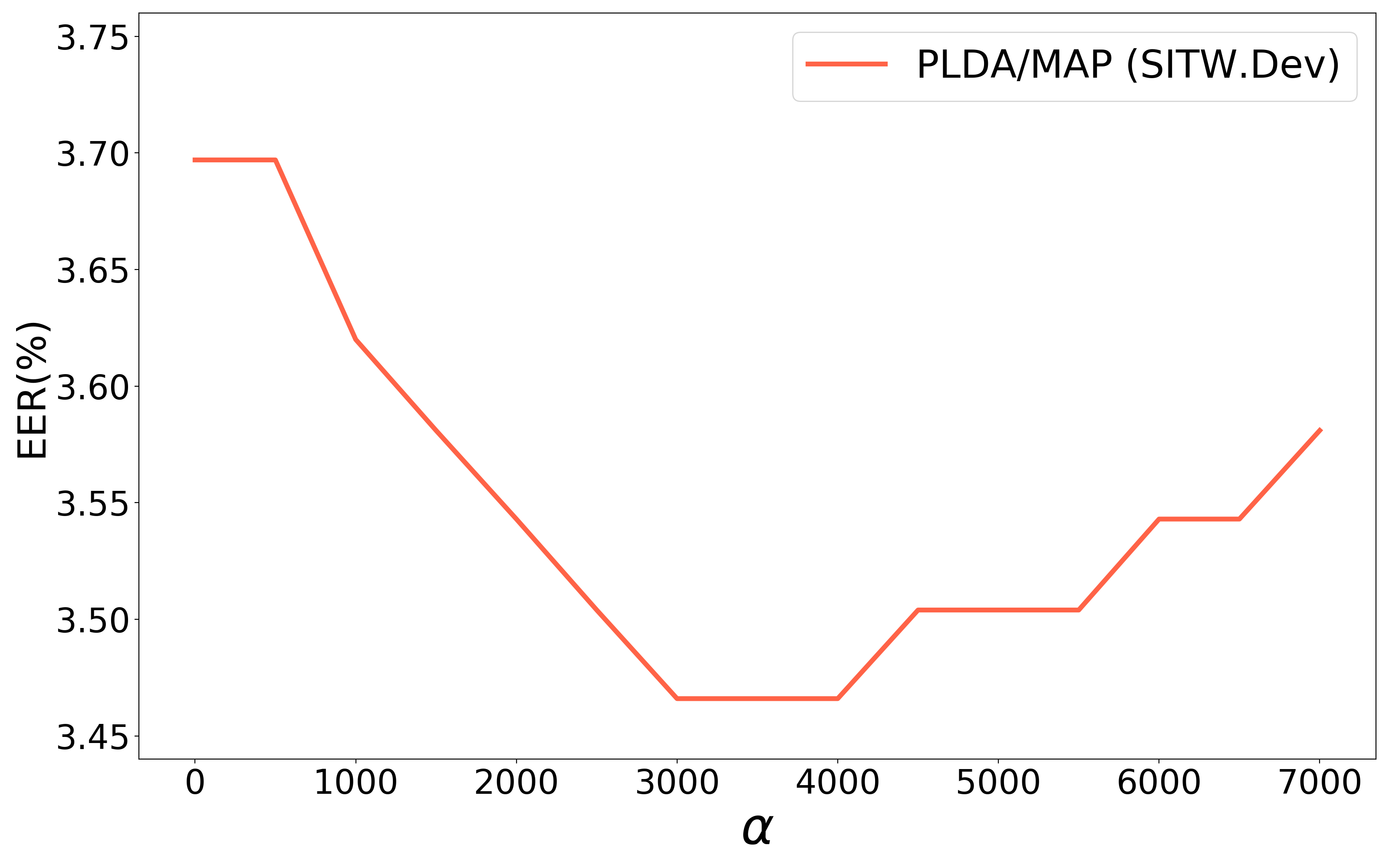
Figure 3: EER results of PLDA/MAP on SITW.Dev with different $\alpha$.

4.3 Detailed results

In this experiment, we choose $\alpha$ using the development sets (SITW.Dev for SITW.Eval test, and HI-MIA.Dev for HI-MIA.Eval test) based on the EER results with PLDA/MAP, and then apply the optimal $\alpha$ to both PLDA/MAP and LN/MAP. The EER results are reported in Table 1.

Firstly, we observe that in almost all the cases, PLDA/MAP outperforms the conventional PLDA. The general improvement obtained by PLDA/MAP implies that the MAP estimation indeed delivers a better between-class covariance.

Secondly, we found that in most tests, LN/MAP clearly outperforms the standard LN. This double confirms that the MAP estimation produces a better between-class covariance. Moreover, since the improvement was obtained by using the prior weight $\alpha$ selected based on PLDA/MAP, we conclude that the priors for PLDA/MAP and LN/MAP are consistent.

Thirdly, we observe that in the LDA[512]-dim tests, PLDA/MAP + LN (system 5) generally outperforms PLDA + LN (system 3), but this is not always the case in the LDA[150]-dim tests. For example, in the SITW test, PLDA/MAP + LN (system 11) performs worse than PLDA + LN (system 9). A possible reason is that with the LN operation, the data statistics has been changed, and so the MAP estimation based on the original statistics may be suboptimal. In general, LN/MAP is more safe than PLDA/MAP as it can improve performance in almost all the cases, though in many cases, PLDA/MAP can deliver more improvement than LN/MAP.

Finally, it seems that combining PLDA/MAP and LN/MAP (system 6) may lead to performance improvement in some cases, but this is not always the case. The improvement, even if it is observed, is not significant. This can be explained again by the suboptimum of the MAP estimation for the data after length normalization.

5 Conclusions

We presented a simple form of MAP estimation for the between-class covariance in the PLDA model. Our derivation shows that under mild conditions, the MAP estimation can be formed as a linear interpolation of the ML estimation obtained by standard PLDA and a prior covariance. We employed the MAP-estimated between-class covariance to both PLDA scoring and length normalization, and interesting performance improvement was obtained. Future work will investigate better strategies to combine MAP estimation and length normalization.

References

- [1] S. Ioffe, “Probabilistic linear discriminant analysis,” in European Conference on Computer Vision (ECCV). Springer, 2006, pp. 531–542.
- [2] S. J. Prince and J. H. Elder, “Probabilistic linear discriminant analysis for inferences about identity,” in 2007 IEEE 11th International Conference on Computer Vision. IEEE, 2007, pp. 1–8.
- [3] A. Sizov, K. A. Lee, and T. Kinnunen, “Unifying probabilistic linear discriminant analysis variants in biometric authentication,” in Joint IAPR International Workshops on Statistical Techniques in Pattern Recognition (SPR) and Structural and Syntactic Pattern Recognition (SSPR). Springer, 2014, pp. 464–475.
- [4] J. P. Campbell, “Speaker recognition: A tutorial,” Proceedings of the IEEE, vol. 85, no. 9, pp. 1437–1462, 1997.
- [5] D. A. Reynolds, “An overview of automatic speaker recognition technology,” in IEEE International Conference on Acoustics, Speech and Signal Processing (ICASSP), vol. 4. IEEE, 2002, pp. IV–4072.
- [6] J. H. Hansen and T. Hasan, “Speaker recognition by machines and humans: A tutorial review,” IEEE Signal processing magazine, vol. 32, no. 6, pp. 74–99, 2015.
- [7] D. Wang, “Remarks on optimal scores for speaker recognition,” arXiv preprint arXiv:2010.04862, 2020.
- [8] P. Kenny, “Bayesian speaker verification with heavy-tailed priors.” in Proceedings of Odyssey: The Speaker and Language Recognition Workshop, 2010, p. 14.
- [9] J. Neyman and E. S. Pearson, “Ix. on the problem of the most efficient tests of statistical hypotheses,” Philosophical Transactions of the Royal Society of London. Series A, Containing Papers of a Mathematical or Physical Character, vol. 231, no. 694-706, pp. 289–337, 1933.
- [10] K. P. Murphy, “Conjugate bayesian analysis of the gaussian distribution,” def, vol. 1, no. 22, p. 16, 2007.
- [11] J. Villalba and N. Brümmer, “Towards fully bayesian speaker recognition: Integrating out the between-speaker covariance,” in Twelfth Annual Conference of the International Speech Communication Association, 2011.
- [12] D. Garcia-Romero and C. Y. Espy-Wilson, “Analysis of i-vector length normalization in speaker recognition systems,” in Proceedings of the Annual Conference of International Speech Communication Association (INTERSPEECH), 2011.
- [13] N. Brümmer, “Bayesian plda,” Tech. Rep., Agnitio Labs, Tech. Rep., 2010.
- [14] N. Dehak, P. J. Kenny, R. Dehak, P. Dumouchel, and P. Ouellet, “Front-end factor analysis for speaker verification,” IEEE Transactions on Audio, Speech, and Language Processing, vol. 19, no. 4, pp. 788–798, 2011.
- [15] J. Villalba and E. Lleida, “Bayesian adaptation of PLDA based speaker recognition to domains with scarce development data,” in Proceedings of Odyssey: The Speaker and Language Recognition Workshop, 2012, pp. 47–54.
- [16] T. Ito, K. Hashimoto, Y. Nankaku, A. Lee, and K. Tokuda, “Speaker recognition based on variational bayesian method,” in Ninth Annual Conference of the International Speech Communication Association, 2008.
- [17] X. Fang et al., “Bayesian distance metric learning on i-vector for speaker verification,” Ph.D. dissertation, Massachusetts Institute of Technology, 2013.
- [18] L. Deng and D. Yu, “Deep learning: methods and applications,” Foundations and trends in signal processing, vol. 7, no. 3–4, pp. 197–387, 2014.
- [19] E. Variani, X. Lei, E. McDermott, I. L. Moreno, and J. Gonzalez-Dominguez, “Deep neural networks for small footprint text-dependent speaker verification,” in IEEE International Conference on Acoustics, Speech and Signal Processing (ICASSP), 2014, pp. 4052–4056.
- [20] L. Li, Y. Chen, Y. Shi, Z. Tang, and D. Wang, “Deep speaker feature learning for text-independent speaker verification,” in Proceedings of the Annual Conference of International Speech Communication Association (INTERSPEECH), 2017, pp. 1542–1546.
- [21] D. Snyder, D. Garcia-Romero, G. Sell, D. Povey, and S. Khudanpur, “X-vectors: Robust DNN embeddings for speaker recognition,” in IEEE International Conference on Acoustics, Speech and Signal Processing (ICASSP). IEEE, 2018, pp. 5329–5333.
- [22] D. Povey, A. Ghoshal, G. Boulianne, L. Burget, O. Glembek, N. Goel, M. Hannemann, P. Motlicek, Y. Qian, P. Schwarz et al., “The Kaldi speech recognition toolkit,” in IEEE workshop on automatic speech recognition and understanding, 2011.
- [23] P. Matějka, O. Plchot, H. Zeinali, L. Mošner, A. Silnova, L. Burget, O. Novotnỳ, and O. Glembek, “Analysis of but submission in far-field scenarios of voices 2019 challenge,” in Proceedings of the Interspeech. 2019, 2019, pp. 15–19.
- [24] J. Villalba, N. Chen, D. Snyder, D. Garcia-Romero, A. McCree, G. Sell, J. Borgstrom, L. P. García-Perera, F. Richardson, R. Dehak, P. A. Torres-Carrasquillo, and N. Dehak, “State-of-the-art speaker recognition with neural network embeddings in NIST SRE18 and speakers in the wild evaluations,” Computer Speech & Language, vol. 60, p. 101026, 2020.
- [25] A. Nagrani, J. S. Chung, and A. Zisserman, “VoxCeleb: a large-scale speaker identification dataset,” in Proceedings of the Annual Conference of International Speech Communication Association (INTERSPEECH), 2017.
- [26] J. S. Chung, A. Nagrani, and A. Zisserman, “VoxCeleb2: Deep speaker recognition,” in Proceedings of the Annual Conference of International Speech Communication Association (INTERSPEECH), 2018, pp. 1086–1090.
- [27] M. McLaren, L. Ferrer, D. Castan, and A. Lawson, “The speakers in the wild (sitw) speaker recognition database.” in Proceedings of the Annual Conference of International Speech Communication Association (INTERSPEECH), 2016, pp. 818–822.
- [28] X. Qin, H. Bu, and M. Li, “HI-MIA: A far-field text-dependent speaker verification database and the baselines,” in IEEE International Conference on Acoustics, Speech and Signal Processing (ICASSP). IEEE, 2020, pp. 7609–7613.