Hidden-Fold Networks: Random Recurrent Residuals Using Sparse Supermasks

Abstract

Deep neural networks (DNNs) are so over-parametrized that recent research has found them to already contain a subnetwork with high accuracy at their randomly initialized state. Finding these subnetworks is a viable alternative training method to weight learning. In parallel, another line of work has hypothesized that deep residual networks (ResNets) are trying to approximate the behaviour of shallow recurrent neural networks (RNNs) and has proposed a way for compressing them into recurrent models. This paper proposes blending these lines of research into a highly compressed yet accurate model: Hidden-Fold Networks (HFNs). By first folding ResNet into a recurrent structure and then searching for an accurate subnetwork hidden within the randomly initialized model, a high-performing yet tiny HFN is obtained without ever updating the weights. As a result, HFN achieves equivalent performance to ResNet50 on CIFAR100 while occupying 38.5x less memory, and similar performance to ResNet34 on ImageNet with a memory size 26.8x smaller. The HFN will become even more attractive by minimizing data transfers while staying accurate when it runs on highly-quantized and randomly-weighted DNN inference accelerators. Code available at: https://github.com/Lopez-Angel/hidden-fold-networks

1 Introduction

Deep neural networks (DNNs) have followed a trend of improvement in accuracy by growing in size. Current popular models, such as residual networks (ResNets) [He et al.(2016)He, Zhang, Ren, and Sun], have tens of millions of parameters. Since off-chip memory access uses much more energy and time than arithmetic computation, data transfers dominate the high cost of DNN processing. Various lines of research have found that these DNNs are much larger than they need to be and have proposed methods for compressing them without harming their accuracy.

Several initiatives have attempted to move the weight of learning away from learning weights. Perturbative neural networks [Juefei-Xu et al.(2018)Juefei-Xu, Naresh Boddeti, and Savvides] proposed substituting convolutional layers with perturbative layers: layers that add fixed random noise to the inputs. Although with lower accuracy, these fixed random modifications together with simple $1$x$1$ convolutional layers are claimed to be enough for learning. A similar approach in this direction showed that learning the parameters of the batch normalization layers while keeping the weights untouched is enough to train a neural network [Frankle et al.(2020)Frankle, Schwab, and Morcos].

Meanwhile, network pruning efforts have made it evident that most popular models are over-parametrized and that large parts of them can be pruned without affecting accuracy [Han et al.(2015)Han, Pool, Tran, and Dally], leading to highly compressed models [Han et al.(2016b)Han, Mao, and Dally] and efficient specialized hardware [Han et al.(2016a)Han, Liu, Mao, Pu, Pedram, Horowitz, and Dally]. It was generally found that the subnetworks resulting from pruning were hard to train from scratch. However, the Lottery Ticket Hypothesis [Frankle and Carbin(2018)] showed that over-parametrized DNNs contain a subnetwork—referred to as a lottery ticket—that can be trained in isolation, overperforming the whole network while being smaller, and requiring fewer iterations to learn. Its authors also proposed a way of finding these subnetworks through the iterative application of three steps: training, pruning, and re-initialization.

This idea was taken a step further with the discovery of hidden-networks (HNNs) [Zhou et al.(2019)Zhou, Lan, Liu, and Yosinski, Ramanujan et al.(2020a)Ramanujan, Wortsman, Kembhavi, Farhadi, and Rastegari]: inside a randomly initialized DNN, there is a hidden subnetwork that, without being trained, achieves similar accuracy to the whole network trained. HNNs can be found by modifying the learning algorithm to optimize a binary mask of the weights—a supermask. Reference [Ramanujan et al.(2020a)Ramanujan, Wortsman, Kembhavi, Farhadi, and Rastegari] proposes an algorithm that finds in ResNet a subnetwork with an accuracy similar to that obtained by training the whole model with dense learned weights. Moreover, a single network can be used for multiple tasks without catastrophic forgetting by finding an appropriate mask for each task or even using combinations of masks for new tasks [Wortsman et al.(2020)Wortsman, Ramanujan, Liu, Kembhavi, Rastegari, Yosinski, and Farhadi].

A different method of compressing networks is found in the hypothesis that ResNets may be approximating unrolled shallow recursive neural networks (RNNs), and that the gains from additional layers correspond to additional recursive iterations [Liao and Poggio(2016), Greff et al.(2016)Greff, Srivastava, and Schmidhuber]. This theory is supported by the authors of [Jastrzębski et al.(2017)Jastrzębski, Arpit, Ballas, Verma, Che, and Bengio], who found that ResNet’s deeper residual blocks are learning to perform iterative refinement of features. Moreover, the work in [Liao and Poggio(2016)] demonstrated that folding ResNet into a 4-layer RNN only had a moderate impact on accuracy.

This theory has roots in neuroscientific observations that have compared the DNNs used for image recognition with biological visual systems. Although DNNs are excellent models of the primate visual cortex [Yamins et al.(2014)Yamins, Hong, Cadieu, Solomon, Seibert, and DiCarlo, Cichy et al.(2016)Cichy, Khosla, Pantazis, Torralba, and Oliva], there are some essential differences. One striking difference is observed at the architectural level: where DNNs typically have tens or hundreds of layers, the visual ventral stream in primate brains has just between four and six layers [Kubilius et al.(2018)Kubilius, Schrimpf, Nayebi, Bear, Yamins, and DiCarlo]. Furthermore, the visual ventral stream layers function in a recurrent way via multiple types of lateral connections [Kar et al.(2019)Kar, Kubilius, Schmidt, Issa, and DiCarlo], unlike popular feed-forward DNN. The hypothesis conjectured on this evidence is that deep learning models are converging to structures similar to the brain’s visual system, and that this convergence can be accelerated by drawing inspiration from these differences. Following these ideas, shallow recurrent models have resulted in both more efficient [Leroux et al.(2018)Leroux, Molchanov, Simoens, Dhoedt, Breuel, and Kautz] and more brain-like [Kubilius et al.(2018)Kubilius, Schrimpf, Nayebi, Bear, Yamins, and DiCarlo] networks.

This paper blends these two research trends into a new type of network: Hidden-Fold Networks (HFNs). First, ResNets are transformed into recursive models through the use of shared weights. Inside this randomly initialized folded structure lies hidden a high-performing network—an HFN. HFNs are unearthed with supermask training. Due to its tiny number of parameters and memory requirements, the proposed method is an exceptional candidate for implementing energy-efficient DNN acceleration hardware.

2 Proposed method: Hidden-Fold Networks

There are three main intuitions for combining into HFN the research trends of learning without updating weights and folding, and for the synergy between their respective techniques.

• Both trends recognize that modern DNNs are over-parametrized and capitalize on it in a way that provides model compression with a minor loss of accuracy.

• Supermask training modifies how weights are treated, whereas folding changes the architecture. The techniques are orthogonal, and therefore it should be possible to combine them without interference.

• ResNet becomes equivalent to a recurrent model when blocks with the same shape are forced to use shared weights. Similarly, the weight initialization used for HNN initializes blocks of the same shape to values of the same modulus. Therefore, both techniques make ResNet more similar to an RNN.

To find an HFN, first a ResNet is initialized randomly. Then, blocks of identical shape within each stage are transformed into recurrent blocks by sharing their weights, except for the BatchNorm parameters. Lastly, instead of updating the weights through backpropagation, the HFN is searched for by training a supermask. The proposed method is formed by four components: architecture, weight initialization, training method, and batch normalization. We describe their details in order.

Architecture — Folded ResNet: This work uses ResNets [He et al.(2016)He, Zhang, Ren, and Sun], converting them into recurrent models via folding [Liao and Poggio(2016)]. ResNets are formed by an input convolutional layer, a main network divided in four stages, and a fully connected output layer, as depicted in Figure 1. Stages are composed of multiple bottleneck blocks, each of which is formed by three convolutional layers. ResNets are named after their total number of convolutional layers, including input and output layers. Since each stage is formed by chaining blocks of the same shape, if their weights are shared, then the function they perform becomes identical. Chaining identical functions is equivalent to applying a function iteratively. Therefore, blocks at each stage can be converted into a recurrent block by sharing their weights, as depicted in Figure 1. This process is the reverse of RNN unrolling and is referred to as folding [Liao and Poggio(2016)].

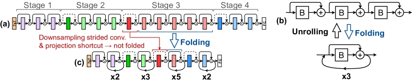
Figure 1: Architecture of HFN (a) ResNet50. ResNets are formed by an input layer, four main stages, and an output layer. (b) Repeated identical instances of a structure are equivalent to a recurrent structure. (c) In this example, identically shaped bottleneck blocks in all stages of ResNet50 are folded.

The difference between stages is the size of the feature maps. To adjust for these dimensional differences, the first block of each stage uses downsampling strided convolution and projection shortcuts. Since this first block is different from the rest, it cannot be folded. These projection blocks could be eliminated, as explored in [Liao and Poggio(2016)] and [Jastrzębski et al.(2017)Jastrzębski, Arpit, Ballas, Verma, Che, and Bengio], but following the intuition that these dimensional transformations correspond to compositional changes in the level of representation [Greff et al.(2016)Greff, Srivastava, and Schmidhuber], this paper keeps them. The rest of the blocks are folded into a single recurrent block, which is iterated a number of times equal to the number of blocks folded (see Figure 1). Since folding makes sense only with more than two blocks per stage, the smallest possible HFNs are ResNet34 and ResNet50. This paper only uses ResNets with bottleneck blocks, and therefore the smallest model used in this paper is ResNet50. The wide variants of ResNet [Zagoruyko and Komodakis(2016)] are also used to consider the depth-width tradeoff.

Weight initialization — Signed Kaiming Constant (SC): Weight initialization is done as [Ramanujan et al.(2020a)Ramanujan, Wortsman, Kembhavi, Farhadi, and Rastegari]. The network initialization process is crucial to find high-performance subnetworks. Good results are achieved using Kaiming initialization [He et al.(2015)He, Zhang, Ren, and Sun], which determines the weight’s distribution by taking into account the network’s shape. Remarkably, even better results are obtained with SC initialization, which initializes all the weights of a layer to the standard deviation $\sigma$ of Kaiming normal distribution, and sets each weight’s sign randomly. In other words, the weights are initialized by sampling uniformly from $\{-\sigma,\sigma\}$, with an independent $\sigma$ for each layer (see Figure 2(a)).

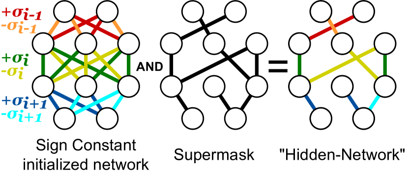
(a) Supermask application

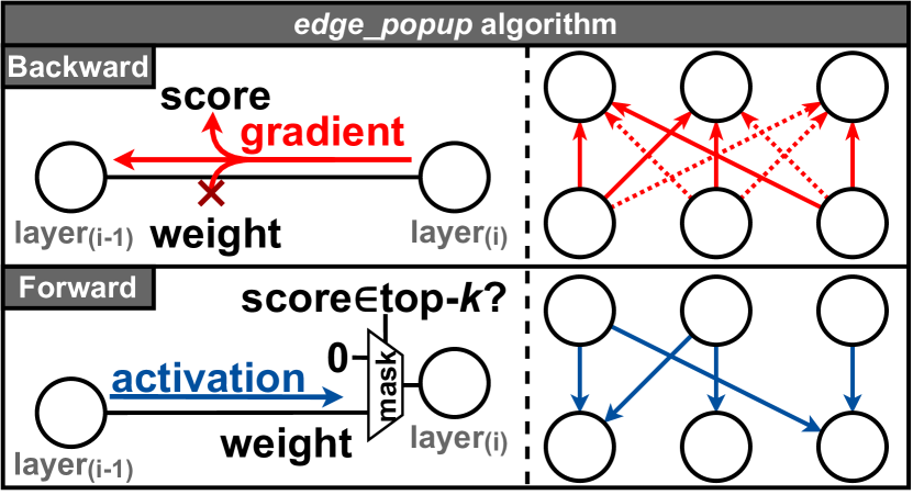
(b) The edge_popup algorithm [Ramanujan et al.(2020a)Ramanujan, Wortsman, Kembhavi, Farhadi, and Rastegari]

Figure 2: (a) The figure shows a supermask applied during inference to a network initialized with SC. Each colour represents each layer’s $\sigma_{i}$ value, with two hues for sign ($-\sigma_{i}$ and $+\sigma_{i}$). (b) Instead of the weights, backpropagation updates the score assigned to each connection. The connections with the top-$k$% scores (solid lines) of each layer form the supermask.

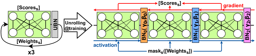
Figure 3: How a folded block is unrolled during training time. In all iterations the same mask and weights are used, and gradients update the same scores. However, an independent affine BatchNorm layer is learned for each iteration.

Training method — Supermasks and edge_popup: An HFN is found by optimizing a supermask with the edge_popup algorithm [Ramanujan et al.(2020a)Ramanujan, Wortsman, Kembhavi, Farhadi, and Rastegari], summarized in Figure 2(b). Each connection is assigned a random score in addition to a weight. In the backwards pass, backpropagation updates the scores instead of the weights, which are left in their randomly initialized state. The top-$k$% highest scores of each convolutional layer are selected in the forward pass, and only their respective connections are used. This is done by constructing a binary mask of the weights—a supermask—in which the positions corresponding to the connections with the top-$k$% highest scores are set to $1$, while the rest are deactivated by assigning them a $0$. As shown in Figure 2(a), the supermask is applied to the weight tensors through an element-wise multiplication (or a logic AND function) during the forward pass, but not during the backward pass, when gradients are propagated to all scores. Thus, top-$k$% is a measure of the model’s density. Scores are unnecessary for inference, but since supermasks are task and weight-dependent, the same random seed must be used for training and inference. This method is used for all convolutional layers of HFN. Folded blocks share a common supermask, which receives gradients from each iteration (see Figure 3).

Batch Normalization [Ioffe and Szegedy(2015)]: Following [Ramanujan et al.(2020a)Ramanujan, Wortsman, Kembhavi, Farhadi, and Rastegari], supermask training uses non-affine BatchNorm, i.e., BatchNorm whose learnable parameters are fixed (bias $\beta=0$ and scale $\gamma=1$). However, folded ResNets suffer from overfitting and exploding layer activations. Reference [Jastrzębski et al.(2017)Jastrzębski, Arpit, Ballas, Verma, Che, and Bengio] suggested using unshared batch normalization (UBN) to alleviate this problem. UBN consists of not sharing batch normalization’s learnable parameters ($\beta$ and $\gamma$) between folded blocks, having a different set for each iteration instead, as exemplified in Figure 3. This approach also proved successful in [Kubilius et al.(2018)Kubilius, Schrimpf, Nayebi, Bear, Yamins, and DiCarlo]. All BatchNorm layers used are non-affine, except for folded blocks, which use UBN.

3 Experiments

This section compares the four methods summarized in Table 1. The experiments described were developed using as a base the PyTorch [Paszke et al.(2019)Paszke, Gross, Massa, Lerer, Bradbury, Chanan, Killeen, Lin, Gimelshein, Antiga, Desmaison, Kopf, Yang, DeVito, Raison, Tejani, Chilamkurthy, Steiner, Fang, Bai, and Chintala] code released by the authors of [Ramanujan et al.(2020a)Ramanujan, Wortsman, Kembhavi, Farhadi, and Rastegari], which can be found at [Ramanujan et al.(2020b)Ramanujan, Wortsman, Kembhavi, Farhadi, and Rastegari]. After confirming the compatibility of supermasks and folding, the optimal HFN configuration is determined by comparing on the same ResNet50. Then, the obtained configuration is used to compare ResNets of different depths and widths. Lastly, the memory advantages of HFN are estimated considering compression on specialized hardware.

Experiments were carried out on the CIFAR100 [Krizhevsky(2009)] and ImageNet [Russakovsky et al.(2015)Russakovsky, Deng, Su, Krause, Satheesh, Ma, Huang, Karpathy, Khosla, Bernstein, Berg, and Fei-Fei] datasets. Since the smallest model used for HFN is the rather big ResNet50, smaller datasets were not used. Unless explicitly stated otherwise, experiments were carried using the following configurations. In experiments using CIFAR100, the $60,000$ images of the set were split into $45,000$ for training, $5,000$ for validation, and $10,000$ for the test set. Data pre-processing was done in the same way as [Ramanujan et al.(2020a)Ramanujan, Wortsman, Kembhavi, Farhadi, and Rastegari]. Models are trained during 200 epochs, using stochastic gradient descent (SGD) with weight decay $0.0005$ and momentum $0.9$. After a warmup of 5 epochs, the learning rate is reduced using cosine annealing starting from $0.1$. The batch size is $128$ for all models except for the original hidden-networks (HNNs) [Ramanujan et al.(2020a)Ramanujan, Wortsman, Kembhavi, Farhadi, and Rastegari], for which the value used is $256$. Experiments using ImageNet use the hyperparameters recommended in [NVIDIA(2021)] for 100 epochs. Reported CIFAR100 accuracies are top-1 test accuracy scores of the models with the highest validation score, while for ImageNet they correspond to top-1 validation accuracy.

Method	Architecture	Training
Standard (“Vanilla”) [He et al.(2016)He, Zhang, Ren, and Sun]	Feedforward	Weights
Folding [Liao and Poggio(2016)]	Recurrent	Weights
Hidden-Networks (HNN) [Ramanujan et al.(2020a)Ramanujan, Wortsman, Kembhavi, Farhadi, and Rastegari]	Feedforward	Supermasks
Hidden-Fold Networks (HFN)	Recurrent	Supermasks

Table 1: Summary of the four methods compared on ResNet in this paper.

3.1 Compatibility of supermasks and folding

The results of applying both supermasks and folding suddenly to the whole network would be hard to interpret. Since starting to fold from the first stages could potentially destroy the feature hierarchy at its base, and there is more evidence for the fourth stage of the visual ventral stream to have a recurrent structure [Kar et al.(2019)Kar, Kubilius, Schmidt, Issa, and DiCarlo], the first set of experiments fold progressively more stages of ResNet50 starting from the last one. Additionally, different combinations of weight initialization (Kaiming normal and SC) and BatchNorm (with and without UBN) are tested. These models were trained on CIFAR100 using dense learned weights (Figure 6(a)) and using supermasks with a fixed density value of top-$k$%$=50\%$ (Figure 6(b)).

The results show a bigger loss in accuracy as more stages are folded, which is recuperated with UBN as expected. In the case of supermask training, both SC initialization and UBN boost the accuracy when used separately, and their effect is stronger when combined. Despite having fewer parameters, SC-initialized HFNs with UBN have similar accuracies to the folded models trained with dense learned weights and higher accuracy than the non-folded HNN-ResNet50. SC and UBN are used for all HFN hereafter.

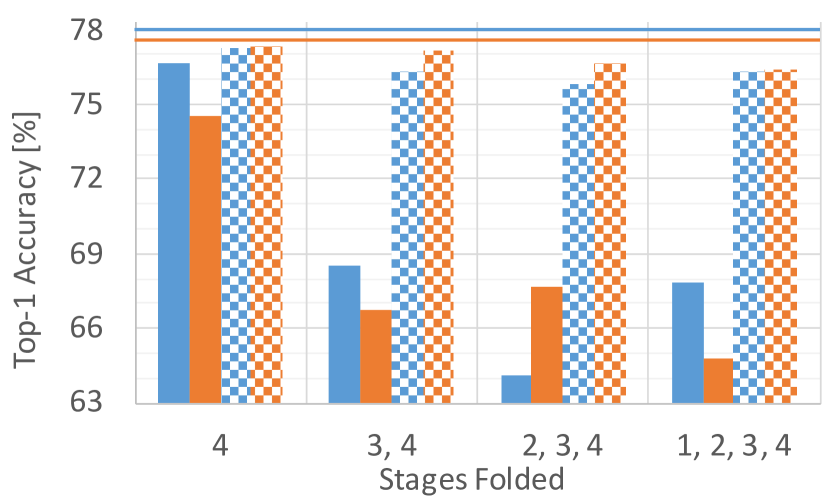
(a) Weight training

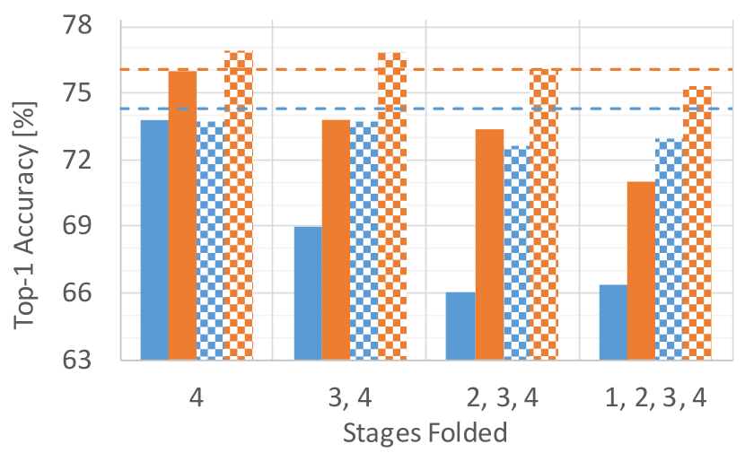
(b) Supermask training

Figure 4: ResNet50 and its hidden and/or folded variants trained on CIFAR100. KN: Kaiming normal; SC: signed Kaiming constant. (a) Vanilla and folding: standard training with weight learning. (b) HNN and HFN: training with supermasks (top-$k$%$=50\%$).

3.2 Tuning supermask density

To check the tradeoffs between accuracy, supermask density, and amount of parameters, the following experiments test a range of top-$k$% values for different configurations of folded stages. Figure LABEL:fig:topk_sweep_layers shows that the optimal top-$k$% values are between $20\%$ and $40\%$ for all cases and that folding only the last two stages (3 and 4) gives the highest accuracy.

These ResNet50 configurations are compared in Figure LABEL:fig:topk_sweep_param with HNN, folding, and vanilla. The different points for each method correspond to the different top-$k$% values in Figure LABEL:fig:topk_sweep_layers. Figure LABEL:fig:topk_sweep_param shows that HFN achieves equivalent or higher accuracy than folding or HNN with fewer parameters. Two conclusions can be drawn from these results: supermask training is as effective as weight learning for recurrent versions of ResNet, and folding ResNet improves the quality of the hidden subnetworks.

Most ResNet weights are located in stages 3 and 4 due to the bigger feature map sizes and their higher number of blocks. Although folding more stages results in smaller models, reducing the supermask density provides higher compression gains with a smaller impact on accuracy. Subsequent experiments only fold stages 3 and 4 since it provides the highest accuracy and a low number of parameters. Additionally, since optimizing top-$k$% between $20\%$ and $40\%$ has a small impact on accuracy, all subsequent experiments use top-$k$%$=30\%$.

3.3 Comparison of different model depths

HFN’s potential is seen more clearly when comparing ResNets of different sizes. Reference [Ramanujan et al.(2020a)Ramanujan, Wortsman, Kembhavi, Farhadi, and Rastegari] showed that a ResNet trained with supermasks has fewer parameters and equivalent accuracy to a deeper vanilla ResNet. Furthermore, a key advantage of folding ResNets into RNNs is that adding layers becomes equivalent to adding iterations, improving performance with few extra parameters, i.e., only those corresponding to additional UBN iterations.

Figure 5(a) compares ResNets of different depths and widths trained with the four discussed methods (vanilla, folding, HNN, and HFN). Models with more than 50 layers were trained for an additional 100 epochs, and all supermasks use top-$k$%$=30\%$. Remarkably, HFNs prove to have the highest accuracies while also being the smallest models. An HFN version of ResNet152 has similar accuracy to ResNet50 while requiring $79.4\%$ fewer parameters, and an HFN-ResNet200 has a higher accuracy with $73.8\%$ fewer parameters.

It is also worth noting that HFN accuracy grows monotonically with the number of layers. This suggests that additional iterations do improve accuracy and support the hypothesis that ResNets approximate unrolled RNNs. Nonetheless, there is also a difference in the number of non-folded blocks between these models. Future work should perform ablation studies to investigate this phenomenon more precisely.

3.4 ImageNet experiments

Figure 5(b) shows the model comparison in Section 3.3, now using the ImageNet dataset. While the results are less impressive than with CIFAR100, HFN still achieves competitive accuracy on ImageNet. HFN-ResNet200 shows similar accuracy to HNN-ResNet101 or ResNet34, with $49.2\%$ and $68.9\%$ less parameters, respectively. It is also significantly more accurate than HNN-ResNet50, which has a similar number of parameters. Even though vanilla ResNet50 achieved better accuracy, its number of parameters is much larger.

Future research on optimal training schedules for supermask training should help HFN to achieve even better results. HFN’s learning converges in all CIFAR100 cases, but in the case of ImageNet the loss kept slowly dropping without reaching convergence in a reasonable amount of epochs. RAdam [Liu et al.(2020)Liu, Jiang, He, Chen, Liu, Gao, and Han] achieved slightly better results than SGD in some cases, and extending training by 100 epochs consistently produced more accurate HFNs.

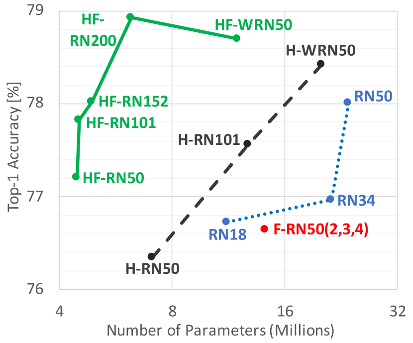
(a) CIFAR100

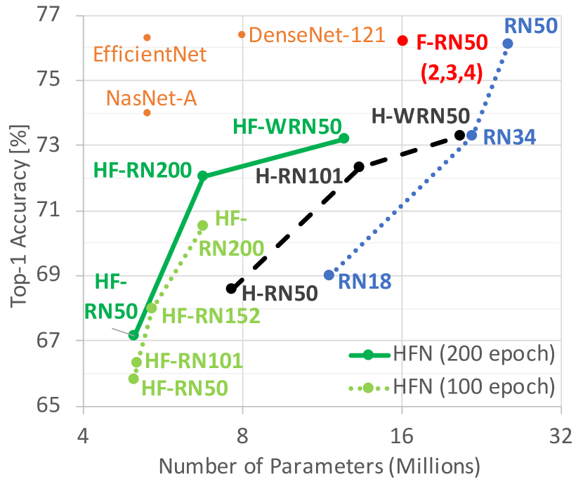
(b) ImageNet

(c) CIFAR100

(d) ImageNet

Figure 5: Top-1 Accuracy of ResNets of different depth and width. Architectures are abbreviated as RN: ResNet; WRN: Wide ResNet. Methods are indicated as F: Folded; H: HNN; HF: HFN; otherwise, vanilla. Numbers in parenthesis indicate folded stages (3 and 4 for all HFN). Models with supermask use top-$k$%$=30\%$. (a) and (b) compare number of parameters, while (c) and (d) compare model memory size. Non-ResNet models in orange.

3.5 Model memory size

All the graphs discussed above compare accuracy based on the number of parameters. Since all the discussed methods use a numeric precision of 32-bit, these graphs can be translated directly into comparisons of the memory required to store each model. However, if considering specialized hardware for inference, a more insightful comparison can be made by exploiting the compression potential of supermasks and SC initialization.

Since the weights are never updated, it is only necessary to store the supermask and the seed for generating the random signs, with the $\sigma$ values calculated on runtime from the network’s shape. Additionally, the supermask only needs one bit per weight to indicate whether if the corresponding connection is part of the subnetwork or not. This straightforward compression vastly reduces the memory needed to store a trained model. Although it is not performed in this paper, supermasks could be compressed even further by exploiting their low density with sparse coding, similarly to [Han et al.(2016b)Han, Mao, and Dally]. In the case of HFN, it is necessary to store the scales and biases of UBN. However, the reduction in weights gained from folding far outweighs the cost of the additional UBN parameters, as it can be appreciated in Figure 5(c) for CIFAR100, and in Figure 5(d) for ImageNet. Figure 5 also compares HFN to other small-sized models (EfficientNet[Tan and Le(2019)], DenseNet[Huang et al.(2017)Huang, Liu, Van Der Maaten, and Weinberger], and NasNet[Zoph et al.(2018)Zoph, Vasudevan, Shlens, and Le]), and shows that although HFN has a lower parameter efficiency, it offers much larger memory gains.

Table 2 shows the effects of the different discussed methods on the same model (ResNet50). Although there is a moderate drop in accuracy, especially in the case of ImageNet, HFN-ResNet50 reduces weight memory storage to a mere $1.95$MB on CIFAR100 and $2.18$MB on ImageNet, small enough to fit in on-chip memory. More importantly, these size gains hold in comparisons of models of similar accuracy, summarized in Table 3. Remarkably, HFN-ResNet152 has similar accuracy to ResNet50 on CIFAR100 despite being $38.5$x smaller, and on ImageNet HFN-ResNet200 has similar accuracy to ResNet34 while being $26.8$x smaller.

Dataset	Model	Top-1 Acc. [%]	Parameters (Millions)	Size [MB]	Size Reduction
CIFAR100	ResNet50	78.01	23.71	94.82	-
	Folded ResNet50 (2,3,4)	76.65	14.24	56.94	1.67x
	HNN-ResNet50	76.35	7.10	3.00	31.66x
	HFN-ResNet50	77.21	4.45	1.95	48.71x
ImageNet	ResNet50	76.10	25.55	102.22	-
	Folded ResNet50 (2,3,4)	76.20	16.08	64.34	1.59x
	HNN-ResNet50	68.60	7.65	3.19	32.04x
	HFN-ResNet50	67.70	5.00	2.18	46.89x

Table 2: Accuracy and size effects of the different methods, compared on the same model.

Dataset	Model	Top-1 Acc. [%]	Parameters (Millions)	Size [MB]	Size Reduction
CIFAR100	ResNet50	78.01	23.71	94.82	-
	HNN-WideResNet50	78.43	20.08	8.37	11.32x
	HFN-ResNet200	78.93	6.21	3.02	31.40x
	HFN-ResNet152	78.02	4.88	2.46	38.54x
ImageNet	ResNet34	73.30	21.78	87.19	-
	HNN-WideResNet50	73.30	20.64	8.60	10.14x
	HFN-WideResNet50	73.19	12.50	5.34	16.33x
	HFN-ResNet200	72.06	6.77	3.25	26.83x

Table 3: Size comparison of models of similar accuracy, using the proposed compression.

4 Discussion

HFNs are accurate models with few and highly reused random parameters. When considering specialized hardware inference accelerators with a random number generator and the capability of operating with binary supermasks, HFNs can be compressed enough to be stored on on-chip SRAM, making off-chip DRAM access for parameters unnecessary. This promises vast energy-efficiency advantages. The bulk of computations used for neural networks consists of energy-hungry multiplications. Still, this cost is minute compared to that of off-chip memory access. In the case of $45$ nm CMOS, a 32 bit floating-point multiplication consumes $3.7$ pJ, while a 32 bit DRAM read costs $640$ pJ [Horowitz(2014), Han et al.(2016a)Han, Liu, Mao, Pu, Pedram, Horowitz, and Dally]. Specialized hardware often operates with reduced numeric precision, making the contrast even starker: a 16 bit floating-point multiplication uses $291$x less energy than DRAM access. Additionally, off-chip memory also suffers from a much longer latency. With random weights, highly compressed binary supermasks, and recurrent connections reusing parameters, memory reads can be reduced to a minimum. Figure 6 shows a comparison of the estimated energy consumed by DRAM access for loading models of similar accuracy, considering an ideal accelerator implemented in $45$ nm CMOS. HFN reduces energy consumption by two orders of magnitude, making it a promising candidate for implementing energy-efficient DNN acceleration hardware.

On the other hand, it shall be noted that HFN is not aimed at CPU/GPU implementation. Since the parameters must be uncompressed at runtime and folding does not change the number or size of convolutions, HFN-ResNet50’s computational cost on standard processors is similar to ResNet50’s. HFN-ResNet152 has similar accuracy to ResNet-50 while using 4.9x less parameters (Table 3, CIFAR100), but its computational cost is almost 3x higher. This tradeoff between computation and size is avoided on specialized hardware, as the computational cost is also reduced by exploiting the model’s sparsity and processing supermasks with binary operations. For software implementations, HFN could be coupled with techniques for reducing computational cost, such as reduced numerical precision, depth-wise separable convolutions [Howard et al.(2017)Howard, Zhu, Chen, Kalenichenko, Wang, Weyand, Andreetto, and Adam], or AdderNets [Chen et al.(2020)Chen, Wang, Xu, Shi, Xu, Tian, and Xu], or by generalizing folding to be compatible with the dense connections of DenseNet [Huang et al.(2017)Huang, Liu, Van Der Maaten, and Weinberger], which would reduce HFN’s number of channels.

Several aspects of supermask training still have to be addressed. Future work should find a method for determining the optimal supermask density a priori or optimizing it during the training process. Furthermore, tuning different density values for each layer could reduce size while increasing accuracy. Alternatively, recent work has proposed using a global density value instead of constraining the density of each layer [Zhou et al.(2021)Zhou, Zhang, Xu, and Zhang]. An initialization method that eliminates the need for normalization, similar to Fixup [Zhang et al.(2019)Zhang, Dauphin, and Ma] but compatible with supermask training, could potentially remove the additional parameters introduced by UBN. Even though HFN achieves remarkable model size reduction, supermask training introduces an additional training cost by using a separate score tensor, which should be addressed. Training ResNet50 on CIFAR100 using 1xNVIDIA GeForce RTX 3090 takes $44$ s per epoch, whereas its HNN and HFN versions take $153$ s and $149$ s respectively.

(a) CIFAR100

(b) ImageNet

Figure 6: Estimation of energy consumed for loading models of similar accuracy from DRAM, considering an ideal $45$ nm CMOS inference accelerator.

5 Conclusion

Hidden-fold networks combine the advances of two recent research trends into a residual network that is small yet accurate. When using an optimal supermask density and training schedule, this method proves beneficial for both original trends: folded models are more accurate when trained with supermasks, and folding ResNets yields more accurate hidden subnetworks than strictly feed-forward models. HFN’s random weights do not need to be stored, as they are substituted with a random seed and sparse binary supermasks that can be highly compressed. Furthermore, recurrent connections can be exploited for reusing parameters. Consequently, HFN can be implemented in specialized hardware with a tiny number of off-chip memory accesses, guaranteeing an energy-efficient and faster system.

References

- [Chen et al.(2020)Chen, Wang, Xu, Shi, Xu, Tian, and Xu] Hanting Chen, Yunhe Wang, Chunjing Xu, Boxin Shi, Chao Xu, Qi Tian, and Chang Xu. Addernet: Do we really need multiplications in deep learning? In Proc. of IEEE Comput. Soc. Conf. Comput. Vis. and Pattern Recognit., pages 1468–1477, 2020.
- [Cichy et al.(2016)Cichy, Khosla, Pantazis, Torralba, and Oliva] Radoslaw M Cichy, Aditya Khosla, Dimitrios Pantazis, Antonio Torralba, and Aude Oliva. Deep neural networks predict hierarchical spatio-temporal cortical dynamics of human visual object recognition. arXiv preprint arXiv:1601.02970, 2016.
- [Frankle and Carbin(2018)] Jonathan Frankle and Michael Carbin. The lottery ticket hypothesis: Finding sparse, trainable neural networks. In Proc. of Int. Conf. Learn. Repr., 2018.
- [Frankle et al.(2020)Frankle, Schwab, and Morcos] Jonathan Frankle, David J Schwab, and Ari S Morcos. Training batchnorm and only batchnorm: On the expressive power of random features in cnns. arXiv preprint arXiv:2003.00152, 2020.
- [Greff et al.(2016)Greff, Srivastava, and Schmidhuber] Klaus Greff, Rupesh K Srivastava, and Jürgen Schmidhuber. Highway and residual networks learn unrolled iterative estimation. arXiv preprint arXiv:1612.07771, 2016.
- [Han et al.(2015)Han, Pool, Tran, and Dally] Song Han, Jeff Pool, John Tran, and William Dally. Learning both weights and connections for efficient neural network. In Proc. of Adv. Neural Inform. Process. Syst., pages 1135–1143, 2015.
- [Han et al.(2016a)Han, Liu, Mao, Pu, Pedram, Horowitz, and Dally] Song Han, Xingyu Liu, Huizi Mao, Jing Pu, Ardavan Pedram, Mark A Horowitz, and William J Dally. EIE: Efficient inference engine on compressed deep neural network. Proc. of Int. Symp. Comp. Archit., 2016a.
- [Han et al.(2016b)Han, Mao, and Dally] Song Han, Huizi Mao, and William J Dally. Deep compression: Compressing deep neural networks with pruning, trained quantization and huffman coding. Proc. of Int. Conf. Learn. Repr., 2016b.
- [He et al.(2015)He, Zhang, Ren, and Sun] Kaiming He, Xiangyu Zhang, Shaoqing Ren, and Jian Sun. Delving deep into rectifiers: Surpassing human-level performance on imagenet classification. In Proc. of IEEE Int. Conf. Comput. Vis., pages 1026–1034, 2015.
- [He et al.(2016)He, Zhang, Ren, and Sun] Kaiming He, Xiangyu Zhang, Shaoqing Ren, and Jian Sun. Deep residual learning for image recognition. In Proc. of IEEE Comput. Soc. Conf. Comput. Vis. and Pattern Recognit., pages 770–778, 2016.
- [Horowitz(2014)] Mark Horowitz. 1.1 computing’s energy problem (and what we can do about it). In Proc. of IEEE Int. Solid-State Circuits Conf., pages 10–14, 2014.
- [Howard et al.(2017)Howard, Zhu, Chen, Kalenichenko, Wang, Weyand, Andreetto, and Adam] Andrew G Howard, Menglong Zhu, Bo Chen, Dmitry Kalenichenko, Weijun Wang, Tobias Weyand, Marco Andreetto, and Hartwig Adam. Mobilenets: Efficient convolutional neural networks for mobile vision applications. arXiv preprint arXiv:1704.04861, 2017.
- [Huang et al.(2017)Huang, Liu, Van Der Maaten, and Weinberger] Gao Huang, Zhuang Liu, Laurens Van Der Maaten, and Kilian Q Weinberger. Densely connected convolutional networks. In Proc. of IEEE Comput. Soc. Conf. Comput. Vis. and Pattern Recognit., pages 4700–4708, 2017.
- [Ioffe and Szegedy(2015)] Sergey Ioffe and Christian Szegedy. Batch normalization: Accelerating deep network training by reducing internal covariate shift. In Proc. of Int. Conf. Mach. Learn., pages 448–456, 2015.
- [Jastrzębski et al.(2017)Jastrzębski, Arpit, Ballas, Verma, Che, and Bengio] Stanisław Jastrzębski, Devansh Arpit, Nicolas Ballas, Vikas Verma, Tong Che, and Yoshua Bengio. Residual connections encourage iterative inference. arXiv preprint arXiv:1710.04773, 2017.
- [Juefei-Xu et al.(2018)Juefei-Xu, Naresh Boddeti, and Savvides] Felix Juefei-Xu, Vishnu Naresh Boddeti, and Marios Savvides. Perturbative neural networks. In Proc. of IEEE Comput. Soc. Conf. Comput. Vis. and Pattern Recognit., pages 3310–3318, 2018.
- [Kar et al.(2019)Kar, Kubilius, Schmidt, Issa, and DiCarlo] Kohitij Kar, Jonas Kubilius, Kailyn Schmidt, Elias B Issa, and James J DiCarlo. Evidence that recurrent circuits are critical to the ventral stream’s execution of core object recognition behavior. Nature Neuroscience, 22(6):974–983, 2019.
- [Krizhevsky(2009)] Alex Krizhevsky. Learning multiple layers of features from tiny images. Technical report, University of Toronto, 2009.
- [Kubilius et al.(2018)Kubilius, Schrimpf, Nayebi, Bear, Yamins, and DiCarlo] Jonas Kubilius, Martin Schrimpf, Aran Nayebi, Daniel Bear, Daniel LK Yamins, and James J DiCarlo. CORnet: Modeling the neural mechanisms of core object recognition. BioRxiv preprint BioRxiv:408385, 2018.
- [Leroux et al.(2018)Leroux, Molchanov, Simoens, Dhoedt, Breuel, and Kautz] Sam Leroux, Pavlo Molchanov, Pieter Simoens, Bart Dhoedt, Thomas Breuel, and Jan Kautz. IamNN: Iterative and adaptive mobile neural network for efficient image classification. arXiv preprint arXiv:1804.10123, 2018.
- [Liao and Poggio(2016)] Qianli Liao and Tomaso Poggio. Bridging the gaps between residual learning, recurrent neural networks and visual cortex. arXiv preprint arXiv:1604.03640, 2016.
- [Liu et al.(2020)Liu, Jiang, He, Chen, Liu, Gao, and Han] Liyuan Liu, Haoming Jiang, Pengcheng He, Weizhu Chen, Xiaodong Liu, Jianfeng Gao, and Jiawei Han. On the variance of the adaptive learning rate and beyond. In Proc. of Int. Conf. Learn. Repr., April 2020.
- [NVIDIA(2021)] NVIDIA. Deeplearningexamples/pytorch/. https://github.com/NVIDIA/DeepLearningExamples/tree/master/PyTorch/Classification/ConvNets/resnet50v1.5, 2021.
- [Paszke et al.(2019)Paszke, Gross, Massa, Lerer, Bradbury, Chanan, Killeen, Lin, Gimelshein, Antiga, Desmaison, Kopf, Yang, DeVito, Raison, Tejani, Chilamkurthy, Steiner, Fang, Bai, and Chintala] Adam Paszke, Sam Gross, Francisco Massa, Adam Lerer, James Bradbury, Gregory Chanan, Trevor Killeen, Zeming Lin, Natalia Gimelshein, Luca Antiga, Alban Desmaison, Andreas Kopf, Edward Yang, Zachary DeVito, Martin Raison, Alykhan Tejani, Sasank Chilamkurthy, Benoit Steiner, Lu Fang, Junjie Bai, and Soumith Chintala. Pytorch: An imperative style, high-performance deep learning library. In Proc. of Adv. Neural Inform. Process. Syst., pages 8024–8035, 2019.
- [Ramanujan et al.(2020a)Ramanujan, Wortsman, Kembhavi, Farhadi, and Rastegari] Vivek Ramanujan, Mitchell Wortsman, Aniruddha Kembhavi, Ali Farhadi, and Mohammad Rastegari. What’s hidden in a randomly weighted neural network? In Proc. of IEEE Comput. Soc. Conf. Comput. Vis. and Pattern Recognit., pages 11893–11902, 2020a.
- [Ramanujan et al.(2020b)Ramanujan, Wortsman, Kembhavi, Farhadi, and Rastegari] Vivek Ramanujan, Mitchell Wortsman, Aniruddha Kembhavi, Ali Farhadi, and Mohammad Rastegari. What’s hidden in a randomly weighted neural network? https://github.com/allenai/hidden-networks, 2020b.
- [Russakovsky et al.(2015)Russakovsky, Deng, Su, Krause, Satheesh, Ma, Huang, Karpathy, Khosla, Bernstein, Berg, and Fei-Fei] Olga Russakovsky, Jia Deng, Hao Su, Jonathan Krause, Sanjeev Satheesh, Sean Ma, Zhiheng Huang, Andrej Karpathy, Aditya Khosla, Michael Bernstein, Alexander C. Berg, and Li Fei-Fei. ImageNet Large Scale Visual Recognition Challenge. Int. J. Comput. Vis., 2015.
- [Tan and Le(2019)] Mingxing Tan and Quoc Le. Efficientnet: Rethinking model scaling for convolutional neural networks. In Proc. of Int. Conf. Mach. Learn., pages 6105–6114, 2019.
- [Wortsman et al.(2020)Wortsman, Ramanujan, Liu, Kembhavi, Rastegari, Yosinski, and Farhadi] Mitchell Wortsman, Vivek Ramanujan, Rosanne Liu, Aniruddha Kembhavi, Mohammad Rastegari, Jason Yosinski, and Ali Farhadi. Supermasks in superposition. Proc. of Adv. Neural Inform. Process. Syst., 33, 2020.
- [Yamins et al.(2014)Yamins, Hong, Cadieu, Solomon, Seibert, and DiCarlo] Daniel LK Yamins, Ha Hong, Charles F Cadieu, Ethan A Solomon, Darren Seibert, and James J DiCarlo. Performance-optimized hierarchical models predict neural responses in higher visual cortex. In Proc. of . Natl. Acad. Sci. U.S.A., pages 8619–8624, 2014.
- [Zagoruyko and Komodakis(2016)] Sergey Zagoruyko and Nikos Komodakis. Wide residual networks. arXiv preprint arXiv:1605.07146, 2016.
- [Zhang et al.(2019)Zhang, Dauphin, and Ma] Hongyi Zhang, Yann N Dauphin, and Tengyu Ma. Fixup initialization: Residual learning without normalization. arXiv preprint arXiv:1901.09321, 2019.
- [Zhou et al.(2019)Zhou, Lan, Liu, and Yosinski] Hattie Zhou, Janice Lan, Rosanne Liu, and Jason Yosinski. Deconstructing lottery tickets: Zeros, signs, and the supermask. In Proc. of Adv. Neural Inform. Process. Syst., pages 3597–3607, 2019.
- [Zhou et al.(2021)Zhou, Zhang, Xu, and Zhang] Xiao Zhou, Weizhong Zhang, Hang Xu, and Tong Zhang. Effective sparsification of neural networks with global sparsity constraint. arXiv preprint arXiv:2105.01571, 2021.
- [Zoph et al.(2018)Zoph, Vasudevan, Shlens, and Le] Barret Zoph, Vijay Vasudevan, Jonathon Shlens, and Quoc V Le. Learning transferable architectures for scalable image recognition. In Proc. of IEEE Comput. Soc. Conf. Comput. Vis. and Pattern Recognit., pages 8697–8710, 2018.