Junction conditions for generalized hybrid metric-Palatini gravity with applications

Abstract

The generalized hybrid metric-Palatini gravity is a theory of gravitation that has an action composed of a Lagrangian given by $f(R,\cal R)$, where $f$ is a function of the metric Ricci scalar $R$ and a new Ricci scalar $\cal R$ formed from a Palatini connection, plus a matter Lagrangian. This theory can be rewritten by trading the new geometric degrees of freedom that appear in $f(R,\cal R)$ into two scalar fields, $\varphi$ and $\psi$, yielding a dynamically equivalent scalar-tensor theory. Given a spacetime theory, the next important step is to find solutions within it. To construct appropriate solutions it is often necessary to know the junction conditions between two spacetime regions at a separation hypersurface $\Sigma$, with each spacetime region being an independent solution of the theory. The junction conditions for the generalized hybrid metric-Palatini gravity are found here, both in the geometric representation and in the scalar-tensor representation, and in addition, for each representation, the junction conditions for a matching with a thin-shell of matter and for a smooth matching at the separation hypersurface are worked out. These junction conditions are then applied to three configurations, namely, a star, a quasistar with a black hole, and a wormhole. The star is made of a Minkowski interior, a thin shell at the interface with all the matter energy conditions being satisfied, and a Schwarzschild exterior with mass $M$, and unlike general relativity where the matching can be performed at any radius $r_{\Sigma}$, for this theory the matching can only be performed at a specific value of the shell radius, namely $r_{\Sigma}=\frac{9M}{4}$, that corresponds to the general relativistic Buchdahl radius. The quasistar with a black hole is made of an interior Schwarzschild black hole surrounded by a thick shell that matches smoothly to a mass $M$ Schwarzschild exterior at the light ring radius $r_{\Sigma e}=3M$, and with the matter energy conditions being satisfied for the whole spacetime. The wormhole is made of some interior with matter that contains the throat, a thin shell at the interface, and a Schwarzschild-AdS exterior with mass $M$ and negative cosmological constant $\Lambda$, with the matter null energy condition being obeyed everywhere within the wormhole.

I Introduction

I.1 Junction conditions in theories of gravitation and applications

In field theories in general, and in particular in theories of gravitation, one has to find the theory’s junctions conditions that match, through a matching surface, a solution in a given region to another solution in a neighbor region. An example is in Newtonian gravitation where, for a boundary surface it is imposed that the gravitational potential and its first derivatives are continuous across the surface, and for a surface layer, i.e., an infinitesimally thin shell, it is imposed that the gravitational potential and its first derivatives on the surface are continuous but its first derivative normal to the surface is discontinuous yielding in a simple case the shell’s mass density, the shell’s pressure being then found through the equation of motion.

General relativity has its own junction conditions. Indeed, to find solutions of the Einstein’s field equations it is often necessary to match two solutions each defined in a given region that join at some hypersurface. The whole spacetime is thus described by two or more regions with different metrics tensors expressed in different coordinate systems. The junction conditions in general relativity for a boundary surface were found by Darmois darmois by imposing that the induced metric across the hypersurface that separates the two spacetime regions must be continuous, and in addition the extrinsic curvature of that hypersurface must also be continuous. Lichnerowicz lichnerowicz also gave a set of conditions to have at a junction which are coordinate dependent, see lake for a comparison between both sets of conditions. For a surface layer, i.e., a thin-shell, Lanczos had a first go at this junction condition problem lanczos1 , which was then picked up by Sen that in matching an interior Minkowski to an exterior Schwarzschild spacetime found, in the context of a thin shell the critical radius that appears in the interior Schwarzschild solution, now called the Buchdahl radius sen . There were further developments by Lanczos himself lanczos2 and then the formalism was definitely closed when Israel put into a Gauss-Codazzi system of equations Israel:1966rt , showing that if the extrinsic curvature is not continuous, then the matching between two regions of spacetime can still be done, but implies the existence of a thin-shell of matter at the junction radius. The thin shell problem was also studied in papa , and Taub gave a very general formalism of which the thin shell fits into taub . Of course, each theory of gravitation has its own junction conditions which must be deduced from the complete set of field equations. The first modified theory of gravitation put forward was general relativity with a cosmological constant term and this theory has the same junction conditions as general relativity itself. In several other theories the junction conditions have been derived. For the Einstein-Cartan theory see firstattemptEC , for the Brans-Dicke theory and other scalar-tensor theories see suffern ; Barrabes:1997kk , for Gauss-Bonnet gravity see Davis:2002gn , for quadratic gravity theories, such as quadratic in the Riemann tensor, Ricci tensor or Ricci scalar $R$, see Senovilla:2014kua ; berezin , for theories with a gravitational Lagrangian density that is a function $f$ of $R$, i.e., $f\left(R\right)$ theories, without torsion see Deruelle:2007pt ; Senovilla:2013vra and with torsion see Vignolo:2018eco , for the hybrid metric-Palatini gravity, which is a development of $f\left(R\right)$ theories now with Lagrangian density $R+f(\cal R)$, where $\cal R$ is a new Ricci scalar derived from a new connection, see olmo , and for another development of $f\left(R\right)$ theories, namely, theories where the Lagrangian density depends on a function of both $R$ and the trace of the stress-energy tensor $T$, i.e., $f\left(R,T\right)$ theories, see Rosa:2021teg .

The junction conditions have a great many number of applications as they are used to derive new solutions and so yield new insights of the corresponding theory of gravitation. In general relativity there are applications to star solutions without and with thin shells and as models for black hole mimickers see lemoszachin ; rosafluid , to gravitational collapse with different interiors and exteriors senovilla1 and gravitational collapse of the Oppenheimer-Snyder in many different coordinate systems, see e.g., silva , to quasistars, i.e., matter surrounded a black hole that shines due to the black hole gravitational field frauendiener , and to wormholes where junctions between one side of the universe and the other side can be performed lemoswormhole1 ; lemoswormholes2 . In Einstein-Cartan theory there are applications of junction conditions to spacetimes containing compact objects luzcarloni , in Brans-Dicke theory there are applications to wormhole solutions sushkov , in Gauss-Bonnet gravity there are applications of thin shells in brane worlds ramirez , in quadratic gravity there are applications to wormholes eiroa , in $f(R)$ theories of gravitation there are applications involving thin shell stars eiroa2 , in the hybrid metric-Palatini extension to $f(R)$ gravity theories there are applications to wormholes bronnikovhybrid , and in the other extension to $f(R)$ that includes the trace of the stress-energy tensor there are applications to stars maurya , to name a few.

I.2 Junction conditions in the generalized hybrid metric-Palatini gravity and applications

The generalized hybrid metric-Palatini gravity is a theory of gravitation that generalizes the hybrid metric-Palatini Lagrangian density $R+f(\cal R)$ into a generic function $f(R,\cal R)$ Tamanini:2013ltp , so that the generalized hybrid metric-Palatini gravity theory is an extra development of $f(R)$ gravity theories. The $f(R,\cal R)$ theory can be written in two representations. One is the geometric representation given by the function $f(R,\cal R)$ itself. The other is the scalar-tensor representation where some of the degrees of freedom in the function $f$ of the geometric fields $R$ and $\cal R$ can be traded for two scalar fields, yielding a dynamically equivalent scalar-tensor theory, in the same manner as the $f\left(R\right)$ theory can be rewritten as a dynamically equivalent scalar-tensor theory with one scalar field. The generalized hybrid metric-Palatini gravity has very interesting features and has been studied in the context of cosmological solutions Rosa:2017jld , wormholes rosa2018 , scalar modes. bombacigno , dynamical systems rosa2019 , stability of Kerr black holes rosabh , cosmic strings Rosa:2021zbk , thick-brane structures rosatb , singularities in cosmological models Rosa:2021ish , weak-field regime Rosa:2021lhc , and double layers applied to wormholes Rosa:2021yym . Junction conditions must be found for any theory of gravitation, including the generalized hybrid metric-Palatini gravity.

In this work, we deduce the junction conditions of the generalized hybrid metric-Palatini gravity. We display these conditions in both the geometrical and the scalar-tensor representations. For each representation the junction conditions for a matching with a thin-shell of matter and for a smooth matching at the separation hypersurface are worked out. We show three applications: stars, quasistars with black holes, and wormholes.

The paper is organized as follows. In Sec. II, we display de action of the theory and the field equations both in the geometrical and in the scalar-tensor representations. In Sec. III, we obtain the sets of junction conditions in the geometrical and in the scalar-tensor representations and in each representation we give the conditions for thin shell matching and for smooth matching. In Sec. IV, we present the junction conditions for static spherically symmetric spacetimes. In Sec. V, the first application of the junction conditions is made to a star thin shell, more precisely, for an inner Minkowski spacetime, a thin shell in the middle, and an outer Schwarzschild spacetime. In Sec. VI, the second application is made to a quasistar with a black hole, it is an application involving smooth matching, an inner Schwarzschild black hole, a mild thin shell at the inner junction, followed by a thick shell that matches smoothly into an outer Schwarzschild vacuum spacetime. In Sec. VII, the third application is presented, to a wormhole involving a thin shell and an outer AdS spacetime. In Sec. VIII, we conclude. The Appendices B and C are used as auxiliary tools to the main text.

II Equations of the generalized hybrid metric-Palatini gravity theory

II.1 Equations of the geometrical representation of the theory

Consider the generalized hybrid metric-Palatini gravity action $S$ given by

$$S=\frac{1}{16\pi}\int_{\Omega}\sqrt{-g}f\left(R,\cal{R}\right)d^{4}x+S_{m},$$ (1)

where we have chosen a system of geometrized units for which the gravitational constant $G$ and the speed of light $c$ are set to one, $\Omega$ is the entire region of the spacetime manifold, $g$ is the determinant of the spacetime metric $g_{ab}$, $R$ is the metric Ricci scalar, $\mathcal{R}$ is the Palatini Ricci scalar, defined by $\mathcal{R}\equiv\mathcal{R}^{ab}g_{ab}$, where the the Palatini Ricci tensor $\mathcal{R}^{ab}$ is defined in terms of an independent connection $\hat{\Gamma}^{c}_{ab}$ as, $\mathcal{R}_{ab}=\partial_{c}\hat{\Gamma}^{c}_{ab}-\partial_{b}\hat{\Gamma}^{c}_{ac}+\hat{\Gamma}^{c}_{cd}\hat{\Gamma}^{d}_{ab}-\hat{\Gamma}^{c}_{ad}\hat{\Gamma}^{d}_{cb}$, $f\left(R,\cal{R}\right)$ is a well behaved function of $R$ and $\cal{R}$, $S_{m}$ is the matter action defined as $S_{m}=\int d^{4}x\sqrt{-g}\;{\cal L}_{m}$ and where ${\cal L}_{m}$ is the matter Lagrangian density considered minimally coupled to the metric $g_{ab}$. Variation of the action (1) with respect to the metric $g_{ab}$ yields the following equation of motion $f_{R}R_{ab}+f_{\cal R}\mathcal{R}_{ab}-\frac{1}{2}g_{ab}f\left(R,\cal{R}\right)-\left(\nabla_{a}\nabla_{b}-g_{ab}\Box\right)f_{R}=8\pi T_{ab}$, where, $f_{R}\equiv\frac{\partial f}{\partial R}$, $f_{\cal R}\equiv\frac{\partial f}{\partial{\cal R}}$, with $f\equiv f\left(R,\cal{R}\right)$, $\nabla_{a}$ is the $\Gamma^{c}_{ab}$ metric connection covariant derivative, with $\Gamma^{a}_{bc}=\frac{1}{2}{g}^{ad}\left(\partial_{b}{g}_{dc}+\partial_{c}{g}_{bd}-\partial_{d}{g}_{bc}\right)$, $\Box=\nabla^{a}\nabla_{a}$ is the d’Alembertian, and $T_{ab}$ is the stress-energy tensor defined as $T_{ab}=-\frac{2}{\sqrt{-g}}\frac{\delta(\sqrt{-g}\,{\cal L}_{m})}{\delta(g^{ab})}$. Varying the action (1) with respect to the independent connection $\hat{\Gamma}^{c}_{ab}$ provides the following equation $\hat{\nabla}_{c}\left(\sqrt{-g}f_{\cal{R}}g^{ab}\right)=0$. where $\hat{\nabla}_{a}$ is the $\hat{\Gamma}^{c}_{ab}$ connection covariant derivative. Now, for the scalar density $\sqrt{-g}$ of weight 1, we have that $\hat{\nabla}_{c}\sqrt{-g}=0$ and so the latter equation simplifies to $\hat{\nabla}_{c}\left(f_{\cal{R}}\,g^{ab}\right)=0$. This means that ${\hat{g}}_{ab}$, defined as ${\hat{g}}_{ab}=f_{\cal{R}}\,g_{ab}$, is a metric compatible with the connection $\hat{\Gamma}^{a}_{bc}$ which then can be written as the following Levi-Civita connection $\hat{\Gamma}^{a}_{bc}=\frac{1}{2}{\hat{g}}^{ad}\left(\partial_{b}{\hat{g}}_{dc}+\partial_{c}{\hat{g}}_{bd}-\partial_{d}{\hat{g}}_{bc}\right)$ where $\partial_{a}$ denotes partial derivative. Note also that ${\hat{g}}_{ab}$ is conformally related to $g_{ab}$ through the conformal factor $f_{\cal{R}}$. This result implies that the two Ricci tensors $R_{ab}$ and $\mathcal{R}_{ab}$, that we assumed to be independent at first, are actually related to each other by $\mathcal{R}_{ab}=R_{ab}-\frac{1}{f_{\mathcal{R}}}\left(\nabla_{a}\nabla_{b}+\frac{1}{2}g_{ab}\Box\right)f_{\mathcal{R}}+\frac{3}{2f_{\mathcal{R}}^{2}}\partial_{a}f_{\mathcal{R}}\partial_{b}f_{\mathcal{R}}$, where again $\Box=\nabla^{c}\nabla_{c}$. This relation allows us to eliminate $\mathcal{R}_{ab}$ from the equation obtained from variation of the action (1) with respect to the metric $g_{ab}$, see above, to get

$$\left(R_{ab}-\nabla_{a}\nabla_{b}+g_{ab}\Box\right)\left(f_{R}+f_{\mathcal{R}}\right)-$$

$$-\frac{3}{2}g_{ab}\Box f_{\mathcal{R}}+\frac{3}{2f_{\mathcal{R}}}\partial_{a}f_{\mathcal{R}}\partial_{b}f_{\mathcal{R}}-\frac{1}{2}g_{ab}f=8\pi T_{ab}\,.$$ (2)

The other equation of motion obtained from varying the action (1) with respect to the independent connection $\hat{\Gamma}^{c}_{ab}$, namely, $\hat{\nabla}_{c}\left(\sqrt{-g}f_{\cal{R}}g^{ab}\right)=0$, see above, can then be swapped by the equation that relates the two Ricci tensors $R_{ab}$ and $\mathcal{R}_{ab}$, namely,

$$\ \mathcal{R}_{ab}=R_{ab}-\frac{1}{f_{\mathcal{R}}}\left(\nabla_{a}\nabla_{b}+\frac{1}{2}g_{ab}\Box\right)f_{\mathcal{R}}+\frac{3}{2f_{\mathcal{R}}^{2}}\partial_{a}f_{\mathcal{R}}\partial_{b}f_{\mathcal{R}}\,,$$ (3)

see above. Considering that $f$ is a function of the two variables $R$ and $\mathcal{R}$, we can write the partial derivatives $\partial_{a}f_{X}$, and the covariant derivatives $\nabla_{a}\nabla_{b}f_{X}$, with $X$ being either $R$ or $\mathcal{R}$, as

$$\partial_{a}f_{X}=f_{XR}\partial_{a}R+f_{X\mathcal{R}}\partial_{a}\mathcal{R}\,,$$

$$\nabla_{a}\nabla_{b}f_{X}=f_{XR}\nabla_{a}\nabla_{b}R+f_{X\mathcal{R}}\nabla_{a}\nabla_{b}\mathcal{R}+$$ (4)

$$+f_{XRR}\partial_{a}R\partial_{b}R+f_{X\mathcal{R}\mathcal{R}}\partial_{a}\mathcal{R}\partial_{b}\mathcal{R}+2f_{XR\mathcal{R}}\partial_{(a}R\partial_{b)}\mathcal{R}\,.$$

These results allow us to expand the terms with derivatives of $f_{R}$ or $f_{\mathcal{R}}$ in Eq. (II.1) and write them as derivatives of either $R$ or $\mathcal{R}$. We do not write the resultant equation here due to its size, it can be found in Appendix A.

II.2 Equations of the scalar representation of the theory

It is sometimes useful to express the action (1) in a scalar-tensor representation. This can be achieved by considering an action with two auxiliary fields, $\alpha$ and $\beta$, respectively, in the following form $S=\frac{1}{16\pi}\int_{\Omega}\sqrt{-g}\Big{[}f\left(\alpha,\beta\right)+\frac{\partial f}{\partial\alpha}\left(R-\alpha\right)+\frac{\partial f}{\partial\beta}\left(\cal{R}-\beta\right)\Big{]}d^{4}x+S_{m}$. Using $\alpha=R$ and $\beta=\mathcal{R}$ we recover action (1). Therefore, we can define two scalar fields as $\varphi=\frac{\partial f}{\partial\alpha}$ and $\psi=-\frac{\partial f}{\partial\beta}$, where the negative sign is put here for convention. The equivalent action is of the form $S=\frac{1}{16\pi}\int_{\Omega}\sqrt{-g}\left[\varphi R-\psi\mathcal{R}-V\left(\varphi,\psi\right)\right]d^{4}x$, where we defined the potential $V\left(\varphi,\psi\right)$ as $V\left(\varphi,\psi\right)=-f\left(\alpha,\beta\right)+\varphi\alpha-\psi\beta$. Taking into account that ${\hat{g}}_{ab}$ is conformally related to $g_{ab}$ through the relation ${\hat{g}}_{ab}=f_{\cal{R}}\,g_{ab}$, and that it can now be written as ${\hat{g}}_{ab}=-\psi\,g_{ab}$, we have that the Ricci scalars $R$ and $\mathcal{R}$ are related through $\mathcal{R}=R+\frac{3}{\psi^{2}}\partial^{a}\psi\partial_{a}\psi-\frac{3}{\psi}\Box\psi$. So, we can replace $\cal{R}$ into the action just derived, to obtain

$$S=\frac{1}{16\pi}\int_{\Omega}\sqrt{-g}\Big{[}\left(\varphi-\psi\right)R-\frac{3}{2\psi}\partial^{a}\psi\partial_{a}\psi$$

$$-V\left(\varphi,\psi\right)\big{]}d^{4}x+S_{m}\,,$$ (5)

where $S_{m}$ is the matter action defined before. Varying the action (II.2) with respect to the metric $g_{ab}$ provides the following gravitational equation

$$\left(\varphi-\psi\right)G_{ab}-\nabla_{a}\nabla_{b}\varphi-\frac{3}{2\psi}\partial_{a}\psi\partial_{b}\psi+\nabla_{a}\nabla_{b}\psi+$$

$$+\left(\Box\varphi-\Box\psi+\frac{3}{4\psi}\partial^{c}\psi\partial_{c}\psi+\frac{1}{2}V\right)g_{ab}=8\pi T_{ab}\,.$$ (6)

Varying the action with respect to the field $\varphi$ and to the field $\psi$ yields, after rearrangements,

$$\Box\varphi+\frac{1}{3}\left(2V-\psi V_{\psi}-\varphi V_{\varphi}\right)=\frac{8\pi T}{3}\,,$$ (7)

and

$$\Box\psi-\frac{1}{2\psi}\partial^{a}\psi\partial_{a}\psi-\frac{\psi}{3}\left(V_{\varphi}+V_{\psi}\right)=0\,,$$ (8)

respectively.

III Junction conditions for the generalized hybrid metric-Palatini gravity theory

III.1 Junction conditions for the geometrical representation of the theory

III.1.1 Matching with a thin-shell at $\Sigma$

Let us denote the whole four-dimensional spacetime by $\mathcal{V}$, which is divided by a hypersurface $\Sigma$ into two regions, $\mathcal{V}^{+}$ and $\mathcal{V}^{-}$. We denote the metric $g_{ab}^{+}$, given in coordinates $x^{a}_{+}$, as the metric in region $\mathcal{V}^{+}$, and the metric $g_{ab}^{-}$, given in coordinates $x^{a}_{-}$, as the metric in region $\mathcal{V}^{-}$, with latin indices running from $0$ to $3$, $0$ being in general a time index. In both sides of $\Sigma$, we define a set of coordinates $y^{\alpha}$, with greek indices running from $0$ to $2$, or some other combination of three indices out of the four latin indices. We define the projection vectors from the four-dimensional regions $\mathcal{V}^{+}$ and $\mathcal{V}^{-}$, to the three-dimensional hypersurface $\Sigma$ as $e^{a}_{\alpha}=\frac{\partial x^{a}}{\partial y^{\alpha}}$. The unit normal vector $n^{a}$ to $\Sigma$ is defined to point in the direction from $\mathcal{V}^{-}$ to $\mathcal{V}^{+}$. We denote by $l$ the proper distance or proper time along the geodesics perpendicular to $\Sigma$. The parameter $l$ is chosen equal to zero at $\Sigma$, is positive in the region $\mathcal{V}^{+}$, and is negative in the region $\mathcal{V}^{-}$. The infinitesimal displacement along the geodesics is $dx^{a}=n^{a}dl$, with $l$ parameterizing the geodesic and the normal $n_{a}$ is here given by $n_{a}=\epsilon\partial_{a}l$, with $\epsilon$ being either $-1$ or $+1$ for $n^{a}$ a timelike or spacelike vector, respectively, so $n_{a}$ satisfies $n^{a}n_{a}=\epsilon$. To match the two regions $\mathcal{V}^{+}$ and $\mathcal{V}^{-}$ through a hypersurface $\Sigma$, the distribution function formalism is in general needed, so we define $\Theta\left(l\right)$ as the Heaviside distribution function, and $\delta\left(l\right)=\partial_{l}\Theta\left(l\right)$ as the Dirac distribution function. For a quantity $X$, we write $X=X^{+}\Theta\left(l\right)+X^{-}\Theta\left(-l\right)$, where the index $+$ indicates that the quantity $X^{+}$ is the value of the quantity $X$ in the region $\mathcal{V}^{+}$, and the index $-$ indicates that the quantity $X^{-}$ is the value of the quantity $X$ in the region $\mathcal{V}^{-}$. The jump of $X$ across $\Sigma$ is denoted by $\left[X\right]=X^{+}|_{\Sigma}-X^{-}|_{\Sigma}$. The normal $n^{a}$ and the tangent vector $e^{a}_{\alpha}$ to $\Sigma$ have zero jump by definition, i.e., $\left[n^{a}\right]=0$ and $\left[e^{a}_{\alpha}\right]=0$.

We now derive the junction conditions for the geometrical representation of the generalized hybrid metric-Palatini gravity. We deal with $g_{ab}$ to start with and only after with $\hat{\Gamma}^{a}_{bc}$. We consider the general case for which a thin-shell arises at the matching hypersurface.

Let us start with $g_{ab}$. To have a spacetime with a line element, and so a metric $g_{ab}$, this has to be properly defined throughout the spacetime. In particular, the metric must have some form of continuity. In the distribution formalism, one writes the metric $g_{ab}$ as

$$g_{ab}=g_{ab}^{+}\Theta(l)+g_{ab}^{-}\Theta(-l)\,.$$ (9)

The derivative of $g_{ab}$ is $\partial_{c}g_{ab}=(\partial_{c}g_{ab}^{+})\Theta(l)+(\partial_{c}g_{ab}^{-})\Theta(-l)+\epsilon\left[g_{ab}\right]n_{c}\delta(l)$. The term proportional to $\delta\left(l\right)$ is problematic, because the Christoffel symbols corresponding to it would have products of the form $\Theta\left(l\right)\delta\left(l\right)$ which are not defined in the distribution formalism. Therefore one has to impose $\left[g_{ab}\right]=0$. Moreover, generically $g_{ab}$ induces a metric on $\Sigma$ which is given $h_{\alpha\beta}=g_{ab}e^{a}_{\alpha}e^{b}_{\beta}$, such that from the exterior the induced metric is $h_{\alpha\beta}^{+}=g_{ab}^{+}e^{a}_{\alpha}e^{b}_{\beta}$ and from the interior the induced metric is $h_{\alpha\beta}^{-}=g_{ab}^{-}e^{a}_{\alpha}e^{b}_{\beta}$. So, for $h_{\alpha\beta}$ to give a continuous metric on $\Sigma$ we must have $h_{\alpha\beta}^{+}-h_{\alpha\beta}^{-}=0$, i.e.,

$$\left[h_{\alpha\beta}\right]=0.$$ (10)

This junction condition is the same as the first junction condition in general relativity, and also should hold generically for many theories of gravitation. Then the derivative of the metric is now

$$\partial_{c}g_{ab}=(\partial_{c}g_{ab}^{+})\Theta(l)+(\partial_{c}g_{ab}^{-})\Theta(-l)\,.$$ (11)

Now, let us analyze the further junction conditions related to $g_{ab}$ that arise in the theory. Notice that Eq. (II.1) depends directly on the function $f$, which can be any general function of $R$ and $\mathcal{R}$. This means that, in general, there will be terms in $f$ that are power-laws or products of $R$ and $\mathcal{R}$. When we write these terms as distribution functions, extra junction conditions will arise in order to prevent the appearance of terms of the form $\Theta\left(l\right)\delta\left(l\right)$, undefined in the distribution formalism. Let us analyze first the zero order derivative term, $R$. In general, the Ricci tensor $R_{ab}$ of the metric $g_{ab}$ can be written in terms of distribution functions as $R_{ab}=R_{ab}^{+}\Theta\left(l\right)+R_{ab}^{-}\Theta\left(-l\right)-\big{(}\epsilon\,e_{a}^{\alpha}e_{b}^{\beta}\left[K_{\alpha\beta}\right]+n_{a}n_{b}\left[K\right]\big{)}\delta\left(l\right)$, where $K_{\alpha\beta}=\nabla_{\alpha}n_{\beta}$ is the extrinsic curvature of $\Sigma$ with $n_{\beta}=e_{\beta}^{b}n_{b}$, and $K=K^{\alpha}_{\alpha}$ is the trace of $K_{\alpha\beta}$. The Ricci scalar is then $R=R^{+}\Theta\left(l\right)+R^{-}\Theta\left(-l\right)-2\epsilon\left[K\right]\delta\left(l\right)$. To avoid the presence of singular terms of the form $\delta\left(l\right)^{2}$ in the products between Ricci scalars, say, in the function $f$, a junction condition arising from this analysis is

$$\left[K\right]=0.$$ (12)

This condition does not appear in general relativity. Using Eq. (12) the Ricci tensor is

$$R_{ab}=R_{ab}^{+}\Theta\left(l\right)+R_{ab}^{-}\Theta\left(-l\right)-\epsilon\left[K_{ab}\right]\delta\left(l\right)\,,$$ (13)

and the Ricci scalar is now

$$R=R^{+}\Theta\left(l\right)+R^{-}\Theta\left(-l\right)\,.$$ (14)

Let us analyze now the first order derivative term $\partial_{a}R$. Computing the partial derivatives of $R$ expressed in Eq. (14) leads to $\partial_{a}R=\partial_{a}R^{+}\Theta\left(l\right)+\partial_{a}R^{-}\Theta\left(-l\right)+\epsilon\left[R\right]n_{a}\delta\left(l\right)$. In the field equations in Eq. (II.1), we can see that due to the existence of the term $\partial_{a}f_{\mathcal{R}}\partial_{b}f_{\mathcal{R}}$, there will be terms depending on products of these derivatives, such as $\partial^{c}R\partial_{c}R$. Given the terms that appear in $\partial_{a}R$ these products would depend on $\delta\left(l\right)^{2}$, which are singular terms, or on $\Theta\left(l\right)\delta\left(l\right)$, which are undefined. Therefore, to avoid the presence of these terms we obtain a junction condition for $R$ as

$$\left[R\right]=0,$$ (15)

Then $\partial_{a}R$ can be written as

$$\partial_{a}R=\partial_{a}R^{+}\Theta\left(l\right)+\partial_{a}R^{-}\Theta\left(-l\right)\,.$$ (16)

Form Eq. (15) we see that $R$ must be continuous across the hypersurface $\Sigma$. We then denote the value of $R$ at $\Sigma$ as $R_{\Sigma}$.

Let us now turn to the independent connection $\hat{\Gamma}$. As we have seen, the Palatini Ricci tensor $\mathcal{R}_{ab}$ is written in terms of $\hat{\Gamma}$ and its derivatives, $\mathcal{R}_{ab}=\partial_{c}\hat{\Gamma}^{c}_{ab}-\partial_{b}\hat{\Gamma}^{c}_{ac}+\hat{\Gamma}^{c}_{cd}\hat{\Gamma}^{d}_{ab}-\hat{\Gamma}^{c}_{ad}\hat{\Gamma}^{d}_{cb}$. Consequently, the Palatini Ricci scalar $\mathcal{R}$ will also depend on $\hat{\Gamma}$ in the same way. As $\mathcal{R}$ is generally present in the field equations through the function $f\left(R,\mathcal{R}\right)$ and its derivatives, extra junction conditions will arise from $\hat{\Gamma}$. Being a fundamental field of the theory, $\hat{\Gamma}$ can be written in the distribution formalism as

$$\hat{\Gamma}^{c}_{ab}=\hat{\Gamma}^{c+}_{ab}\Theta\left(l\right)+\hat{\Gamma}^{c-}_{ab}\Theta\left(-l\right)\,,$$ (17)

where $\delta$ terms are not present to avoid the presence of undefined terms. Defining the extrinsic curvature written in terms of the independent connection $\hat{\Gamma}$ as $\mathcal{K}_{ab}=e_{a}^{\alpha}e_{b}^{\beta}\hat{\nabla}_{\alpha}n_{\beta}$, where $\hat{\nabla}$ is the covariant derivative on the boundary with respect to $\hat{\Gamma}$, the trace of $\mathcal{K}_{ab}$ as $\mathcal{K}$, and following the previous arguments for $R_{ab}$ and $R$ that led Eq. (12), we obtain

$$\left[\mathcal{K}\right]=0\,.$$ (18)

Then, the Ricci tensor is

$$\mathcal{R}_{ab}=\mathcal{R}_{ab}^{+}\Theta\left(l\right)+\mathcal{R}_{ab}^{-}\Theta\left(-l\right)-\epsilon\left[{\mathcal{K}}_{ab}\right]\delta\left(l\right)\,.$$ (19)

and with the help of Eq. (18) the corresponding Ricci scalar is

$$\mathcal{R}=\mathcal{R}^{+}\Theta\left(l\right)+\mathcal{R}^{-}\Theta\left(-l\right).$$ (20)

Let us now work with $\partial_{a}\mathcal{R}$. Computing the partial derivatives of $\mathcal{R}$ expressed in Eq. (20) leads to $\partial_{a}\mathcal{R}=\partial_{a}\mathcal{R}^{+}\Theta\left(l\right)+\partial_{a}\mathcal{R}^{-}\Theta\left(-l\right)+\epsilon\delta\left(l\right)\left[\mathcal{R}\right]n_{a}$. In the field equations in Eq. (II.1), we can see that due to the existence of the term $\partial_{a}f_{\mathcal{R}}\partial_{b}f_{\mathcal{R}}$, there will be terms depending on products of these derivatives, such as $\partial^{c}{\mathcal{R}}\partial_{c}{\mathcal{R}}$. Given the terms that appear in $\partial_{a}\mathcal{R}$, again these products would depend on $\delta\left(l\right)^{2}$, which are singular terms, or on $\Theta\left(l\right)\delta\left(l\right)$, which are undefined. Therefore, to avoid the presence of these terms we obtain the junction conditions for $\mathcal{R}$ as

$$\left[\mathcal{R}\right]=0.$$ (21)

Then $\partial_{a}\mathcal{R}$ can be written as

$$\partial_{a}\mathcal{R}=\partial_{a}\mathcal{R}^{+}\Theta\left(l\right)+\partial_{a}\mathcal{R}^{-}\Theta\left(-l\right)\,.$$ (22)

Form Eq. (21) we see that $\mathcal{R}$ must be continuous across the hypersurface $\Sigma$. We then denote the value of $\mathcal{R}$ at $\Sigma$ as $\mathcal{R}_{\Sigma}$. Clearly, Eqs. (15) and (21), imply that the terms with first derivatives of $R$ and $\mathcal{R}$, see Eqs. (16) and (22) are regular.

We now turn to the jumps of the derivatives of $R$ and $\mathcal{R}$. These jumps are not independent of each other, and the relationship between them can be obtained from Eq. (3). To find this relationship, let us first write the second order derivatives of $R$ and $\mathcal{R}$, i.e., the terms $\nabla_{a}\nabla_{b}R$, $\Box R$, $\nabla_{a}\nabla_{b}\mathcal{R}$, and $\Box\mathcal{R}$, in the distribution formalism. The second order term $\nabla_{a}\nabla_{b}R$ can be generically written in the distribution formalism as

$$\nabla_{a}\nabla_{b}R =\nabla_{a}\nabla_{b}R_{+}\Theta\left(l\right)+\nabla_{a}\nabla_{b}R_{-}\Theta\left(-l\right)+$$ (23)

$$\epsilon n_{a}\left[\partial_{b}R\right]\delta\left(l\right)\,,$$

and then $\Box R=\Box R_{+}\Theta\left(l\right)+\Box R_{-}\Theta\left(-l\right)+n^{a}\left[\partial_{a}R\right]\delta\left(l\right)$. Likewise, the second order term $\nabla_{a}\nabla_{b}{\mathcal{R}}$ can be generically written in the distribution formalism as

$$\nabla_{a}\nabla_{b}{\mathcal{R}} =\nabla_{a}\nabla_{b}{\mathcal{R}}_{+}\Theta\left(l\right)+\nabla_{a}\nabla_{b}{\mathcal{R}}_{-}\Theta\left(-l\right)+$$ (24)

$$\epsilon n_{a}\left[\partial_{b}{\mathcal{R}}\right]\delta\left(l\right)\,,$$

and then, $\Box{\mathcal{R}}=\Box{\mathcal{R}}_{+}\Theta\left(l\right)+\Box{\mathcal{R}}_{-}\Theta\left(-l\right)+\epsilon n^{a}\left[\partial_{a}{\mathcal{R}}\right]\delta\left(l\right)$. Taking the trace of Eq. (3) written in terms of the distribution functions and using the expansions given in Eqs. (23) and  (24) for the second order derivatives, one obtains

$$f_{\mathcal{R}R}n^{a}\left[\partial_{a}R\right]+f_{\mathcal{R}\mathcal{R}}n^{a}\left[\partial_{a}\mathcal{R}\right]=0\,,$$ (25)

which is the equation that relates the jumps of the derivatives of $R$ and $\mathcal{R}$.

Given the second order derivatives of $R$ and $\mathcal{R}$, in the distribution formalism, see Eqs. (23) and  (24), the left-hand side of the field equation in Eq. (II.1) thus depends on terms proportional to the delta function $\delta\left(l\right)$. These terms are associated with the presence of a thin-shell at the separation hypersurface $\Sigma$. To find the properties of the thin shell, i.e., the stress-energy tensor for this hypersurface, let us write the stress-energy tensor in the geometrical representation $T_{{\rm gr}\hskip 0.85355ptab}$, which we write simply as $T_{ab}$ to shorten the notation, as a distribution function of the form

$$T_{ab}=T_{ab}^{+}\Theta\left(l\right)+T_{ab}^{-}\Theta\left(-l\right)+\delta\left(l\right)S_{ab},$$ (26)

where $T_{ab}^{+}$ is the stress-energy tensor in the geometrical representation in the region $\mathcal{V}^{+}$, $T_{ab}^{-}$ is the stress-energy tensor in the geometrical representation in the region $\mathcal{V}^{-}$, and where $S_{ab}$ is the 4-dimensional stress-energy tensor of the thin shell in the geometrical representation, which can be written as a 3-dimensional tensor at $\Sigma$ as

$$S_{ab}=S_{\alpha\beta}e^{\alpha}_{a}e^{\beta}_{b}.$$ (27)

With these considerations, the $\delta\left(l\right)$ terms in the field equations Eq. (II.1) at the hypersurface $\Sigma$ can be written as $-\left(f_{R}+f_{\mathcal{R}}\right)\epsilon\left[K_{\alpha\beta}\right]+h_{\alpha\beta}\left[\left(f_{RR}-\frac{1}{2}f_{\mathcal{R}R}\right)\epsilon n^{c}\left[\partial_{c}R\right]+\left(f_{R\mathcal{R}}-\frac{1}{2}f_{\mathcal{R}\mathcal{R}}\right)\epsilon n^{c}\left[\partial_{c}\mathcal{R}\right]\right]\break=8\pi S_{\alpha\beta}$, where $f$ and its derivatives are evaluated considering $R=R_{\Sigma}$ and $\mathcal{R}=\mathcal{R}_{\Sigma}$. In this step, we used the property $n_{a}e^{a}_{\alpha}=0$. The jumps of the derivatives of $R$ and $\mathcal{R}$ are not independent of each other, and the relationship between them has been obtained, see Eq. (25). Inserting Eq. (25) into the expression just written for $S_{\alpha\beta}$ and raising one index using the inverse induced metric $h^{\alpha\beta}$, yields finally the equation that allows to compute the stress-energy tensor of the thin shell as

$$\epsilon\delta_{\alpha}^{\beta}n^{c}\left[\partial_{c}R\right]\left(f_{RR}-\frac{f_{\mathcal{R}R}^{2}}{f_{\mathcal{R}\mathcal{R}}}\right)-\left(f_{R}+f_{\mathcal{R}}\right)\epsilon\left[K_{\alpha}^{\beta}\right]=8\pi S_{\alpha}^{\beta}\,,$$ (28)

where $\delta_{\alpha}^{\beta}=h^{\beta\gamma}h_{\gamma\alpha}$ is the identity matrix.

Several remarks should be done. Note that the trace of the extrinsic curvature $K$ can be written in terms of the trace of the extrinsic curvature $\mathcal{K}$ and the conformal factor $f_{\mathcal{R}}$ as $\mathcal{K}=K+n^{c}\partial_{c}f_{\mathcal{R}}/f_{\mathcal{R}}$. The conformal factor $f_{\mathcal{R}}\left(R,\mathcal{R}\right)$ is a function of only $R$ and $\mathcal{R}$, and both these variables must be continuous to satisfy their own junction conditions in Eqs. (15) and (21). Consequently, we have $\left[f_{\mathcal{R}}\left(R,\mathcal{R}\right)\right]=0$. Thus, taking the jump of $\mathcal{K}$, expanding $\partial_{c}f_{\mathcal{R}}$ in terms of $\partial_{c}R$ and $\partial_{c}\mathcal{R}$, and using Eqs. (12) and (25), we recover Eq. (18). Thus, these two junction conditions are also not independent.

To conclude, the full set of independent junction conditions of the theory in the geometrical representation for a matching with a shell is thus

$$\left[h_{\alpha\beta}\right]=0\,,$$

$$\left[K\right]=0\,,$$

$$\left[R\right]=0\,,$$ (29)

$$\left[\mathcal{R}\right]=0\,,$$

$$\epsilon\delta_{\alpha}^{\beta}n^{c}\left[\partial_{c}R\right]\left(f_{RR}-\frac{f_{\mathcal{R}R}^{2}}{f_{\mathcal{R}\mathcal{R}}}\right)-\left(f_{R}+f_{\mathcal{R}}\right)\epsilon\left[K_{\alpha}^{\beta}\right]=8\pi S_{\alpha}^{\beta}\,,$$

$$f_{\mathcal{R}R}n^{a}\left[\partial_{a}R\right]+f_{\mathcal{R}\mathcal{R}}n^{a}\left[\partial_{a}\mathcal{R}\right]=0\,,$$

so composed of six equations. Note that in the case that $f\left(R,\mathcal{R}\right)$ reduces to an $f(R)$ theory the fourth and sixth equations of Eq. (III.1.1) are identically zero.

III.1.2 Matching smoothly at $\Sigma$

We have obtained the junction conditions for which two spacetimes, $\mathcal{V}^{+}$ and $\mathcal{V}^{-}$, can be matched at a given separation hypersurface $\Sigma$ with the presence of a thin-shell at $\Sigma$ described by a surface stress-energy tensor $S_{\alpha}^{\beta}$. If $S_{\alpha}^{\beta}$ vanishes, the matching between the two spacetimes is smooth, i.e., without the need for a thin shell at the separation hypersurface. A smooth matching between $\mathcal{V}^{+}$ and $\mathcal{V}^{-}$ can be achieved by imposing another set of conditions on the geometrical variables. Indeed, the presence of the thin-shell is associated with the term in the stress-energy tensor proportional to $\delta\left(l\right)$ when written in the distribution formalism, which is then reflected in the field equations.

For a smooth matching, i.e., for a matching without a thin-shell, one must guarantee that the terms proportional to $\delta\left(l\right)$ vanish. Let us now derive the conditions for such to happen in the geometrical representation of the theory.

The form of the metric for the whole spacetime as given in Eq. (9) is still valid for a smooth matching, so following the same procedure we have again that $h_{\alpha\beta}$, the induced metric on $\Sigma$, has no jump,

$$\left[h_{\alpha\beta}\right]=0.$$ (30)

Now, the Ricci tensor $R_{ab}$ of the metric $g_{ab}$ can be written in terms of distribution functions as $R_{ab}=R_{ab}^{+}\Theta\left(l\right)+R_{ab}^{-}\Theta\left(-l\right)-\big{(}\epsilon\,e_{a}^{\alpha}e_{b}^{\beta}\left[K_{\alpha\beta}\right]+n_{a}n_{b}\left[K\right]\big{)}\delta\left(l\right)$, where $K_{\alpha\beta}=\nabla_{\alpha}n_{\beta}$ is the extrinsic curvature of $\Sigma$ with $n_{\beta}=e_{\beta}^{b}n_{b}$, and $K=K^{\alpha}_{\alpha}$ is the trace of $K_{\alpha\beta}$. But the field equation Eq. (II.1) has an $R_{ab}$ term and so in general it would possess a term proportional to $\delta\left(l\right)$ which cannot be present for a smooth matching. To avoid the presence of this term in the field equation Eq. (II.1), one must impose that the jump of the extrinsic curvature $K_{ab}=e_{a}^{\alpha}e_{b}^{\beta}K_{\alpha\beta}$ must vanish, i.e., one obtains the following junction condition,

$$\left[K_{\alpha\beta}\right]=0.$$ (31)

Since $\left[K_{\alpha\beta}\right]=0$ it implies directly that its trace vanishes, $\left[K\right]=0$. Moreover $\left[K_{\alpha\beta}\right]=0$ implies that $R_{ab}=R_{ab}^{+}\Theta\left(l\right)+R_{ab}^{-}\Theta\left(-l\right)$, and thus $R=R^{+}\Theta\left(l\right)+R^{-}\Theta\left(-l\right)$. As we have done previously, computing then the partial derivatives of $R$ one finds $\partial_{a}R^{+}\Theta\left(l\right)+\partial_{a}R^{-}\Theta\left(-l\right)+\epsilon\left[R\right]n_{a}\delta\left(l\right)$, which when put into the terms $\partial_{a}f_{\mathcal{R}}\partial_{b}f_{\mathcal{R}}$ in the field equation, Eq. (II.1), gives rise to terms depending on products of these derivatives, such as $\partial^{c}R\partial_{c}R$, which are singular terms, or on $\Theta\left(l\right)\delta\left(l\right)$, which are undefined, and cannot be present in any matching, including a smooth matching, and so this leads to

$$\left[R\right]=0,$$ (32)

From Eq. (32) we see that $R$ must be continuous across the hypersurface $\Sigma$. We then denote the value of $R$ at $\Sigma$ as $R_{\Sigma}$. Also from Eq. (32) one finds that $\partial_{a}R$ can be written as $\partial_{a}R=\partial_{a}R^{+}\Theta\left(l\right)+\partial_{a}R^{-}\Theta\left(-l\right)$

Turning to the independent connection $\hat{\Gamma}$, as we have seen the Palatini Ricci tensor $\mathcal{R}_{ab}$ is written in terms of $\hat{\Gamma}$ and its derivatives, $\mathcal{R}_{ab}=\partial_{c}\hat{\Gamma}^{c}_{ab}-\partial_{b}\hat{\Gamma}^{c}_{ac}+\hat{\Gamma}^{c}_{cd}\hat{\Gamma}^{d}_{ab}-\hat{\Gamma}^{c}_{ad}\hat{\Gamma}^{d}_{cb}$. The Ricci tensor $\mathcal{R}_{ab}$ can be written in terms of distribution functions as $\mathcal{R}_{ab}=\mathcal{R}_{ab}^{+}\Theta\left(l\right)+\mathcal{R}_{ab}^{-}\Theta\left(-l\right)-\big{(}\epsilon\,e_{a}^{\alpha}e_{b}^{\beta}\left[\mathcal{K}_{\alpha\beta}\right]+n_{a}n_{b}\left[\mathcal{K}\right]\big{)}\delta\left(l\right)$, where $\mathcal{K}_{\alpha\beta}=\nabla_{\alpha}n_{\beta}$ is the extrinsic curvature of $\Sigma$ with $n_{\beta}=e_{\beta}^{b}n_{b}$, and $\mathcal{K}=\mathcal{K}^{\alpha}_{\alpha}$ is the trace of $\mathcal{K}_{\alpha\beta}$.

Let us now look at Eq. (II.1) again. We have already concluded that the term $R_{ab}$ does not have any terms proportional to $\delta\left(l\right)$ and also for a smooth matching $T_{ab}$ cannot have terms proportional to $\delta\left(l\right)$. Thus, the the differential terms on $f_{\mathcal{R}}$ in Eq. (II.1) cannot have terms proportional to $\delta\left(l\right)$. Then, from Eq. (3) it is clear that generically $\mathcal{R}_{ab}$ cannot have a term proportional to $\delta\left(l\right)$. Thus, the jump of the extrinsic curvature $\mathcal{K}_{ab}=e_{a}^{\alpha}e_{b}^{\beta}\mathcal{K}_{\alpha\beta}$ must vanish, i.e., one obtains the following junction condition,

$$\left[\mathcal{K}_{\alpha\beta}\right]=0.$$ (33)

Since $\left[\mathcal{K}_{\alpha\beta}\right]=0$ it implies directly that its trace vanishes, $\left[\mathcal{K}\right]=0$. Moreover $\left[\mathcal{K}_{\alpha\beta}\right]=0$ implies that $\mathcal{R}_{ab}=\mathcal{R}_{ab}^{+}\Theta\left(l\right)+\mathcal{R}_{ab}^{-}\Theta\left(-l\right)$, and thus ${\mathcal{R}}=\mathcal{R}^{+}\Theta\left(l\right)+\mathcal{R}^{-}\Theta\left(-l\right)$. As we have done previously, computing then the partial derivatives of $R$ one finds $\partial_{a}\mathcal{R}^{+}\Theta\left(l\right)+\partial_{a}\mathcal{R}^{-}\Theta\left(-l\right)+\epsilon\left[\mathcal{R}\right]n_{a}\delta\left(l\right)$, which when put in the field equations into the terms $\partial_{a}f_{\mathcal{\mathcal{missing}}}R\partial_{b}f_{\mathcal{\mathcal{missing}}}R$ in the field equation, Eq. (II.1), gives rise to terms depending on products of these derivatives, such as $\partial^{c}\mathcal{R}\partial_{c}\mathcal{R}$, which are singular terms, or on $\Theta\left(l\right)\delta\left(l\right)$, which are undefined, and cannot be present in any matching, including a smooth matching, and so this leads to

$$\left[\mathcal{R}\right]=0,$$ (34)

From Eq. (34) we see that $\mathcal{R}$ must be continuous across the hypersurface $\Sigma$. We then denote the value of $\mathcal{R}$ at $\Sigma$ as $\mathcal{R}_{\Sigma}$. Also from Eq. (34) one finds that $\partial_{a}\mathcal{R}$ can be written as $\partial_{a}\mathcal{R}=\partial_{a}\mathcal{R}^{+}\Theta\left(l\right)+\partial_{a}\mathcal{R}^{-}\Theta\left(-l\right)$.

Furthermore, due to the presence of the second-order derivative terms $\nabla_{a}\nabla_{b}f_{X}$ and $\Box f_{X}$ in Eq. (II.1), there will be second-order derivative terms of both $R$ and $\mathcal{R}$ in the field equations. These second-order derivatives are $\nabla_{a}\nabla_{b}R=\nabla_{a}\nabla_{b}R_{+}\Theta\left(l\right)+\nabla_{a}\nabla_{b}R_{-}\Theta\left(-l\right)+\epsilon n_{a}\left[\partial_{b}R\right]\delta\left(l\right)$ and $\Box R=\Box R_{+}\Theta\left(l\right)+\Box R_{-}\Theta\left(-l\right)+n^{a}\left[\partial_{a}R\right]\delta\left(l\right)$, see Eq. (23) and the one following it, and the same expressions for $\nabla_{a}\nabla_{b}{\mathcal{R}}$ and $\Box\mathcal{R}$, see Eq. (24) and the one following it, and they have terms proportional to $\delta\left(l\right)$. To avoid the presence of these terms in order to have a smooth matching, on has to impose that the jump of the first-order derivatives of $R$ and $\mathcal{R}$ vanish, i.e., we obtain the two following junction conditions

$$\left[\partial_{a}R\right]=0,$$ (35)

$$\left[\partial_{a}\mathcal{R}\right]=0.$$ (36)

Several remarks should be done. Note that the extrinsic curvature $\mathcal{K}_{\alpha\beta}$ can be written in terms of the extrinsic curvature $K_{\alpha\beta}$ and the conformal factor $f_{\mathcal{R}}$ as $\mathcal{K}_{\alpha\beta}=K_{\alpha\beta}-X^{c}_{ab}n_{c}$, where $X^{c}_{ab}=\frac{1}{2f_{\mathcal{R}}}\left(g^{c}_{b}\partial_{a}+g^{c}_{a}\partial_{b}-g_{ab}\partial^{c}\right)f_{\mathcal{R}}$. The conformal factor $f_{\mathcal{R}}\left(R,\mathcal{R}\right)$ is a function of only $R$ and $\mathcal{R}$, and both these variables must be continuous to satisfy their own junction conditions in Eqs. (32) and (34). Consequently, we have $\left[f_{\mathcal{R}}\left(R,\mathcal{R}\right)\right]=0$. Thus, taking the jump of $\mathcal{K}_{\alpha\beta}$, expanding $\partial_{c}f_{\mathcal{R}}$ in terms of $\partial_{c}R$ and $\partial_{c}\mathcal{R}$, and using Eqs. (30), (35) and (36), we recover Eq. (31). Thus, these two junction conditions are not independent.

To conclude, the full set of independent junction conditions of the theory in the geometrical representation for a smooth matching is thus

$$\left[h_{\alpha\beta}\right]=0\,,$$

$$\left[K_{\alpha}^{\beta}\right]=0\,,$$

$$\left[R\right]=0\,,$$ (37)

$$\left[\mathcal{R}\right]=0\,,$$

$$\left[\partial_{a}R\right]=0\,,$$

$$\left[\partial_{a}\mathcal{R}\right]=0\,,$$

so composed of six equations. Note, that the same set of extra junction conditions can be obtained from the general set in Eq. (III.1.1) by setting $S_{\alpha\beta}=0$. In this case, since the factors depending on derivatives of the function $f$ are generally nonzero, putting the second equation into the trace of the fifth equation of Eq. (III.1.1) yields the fifth equation of Eq. (III.1.2), which on putting it back into the fifth equation of Eq. (III.1.1) yields the second equation of Eq. (III.1.2). Note in addition that in the case that $f\left(R,\mathcal{R}\right)$ reduces to an $f(R)$ theory the fourth and sixth equations of Eq. (III.1.2) are identically zero.

III.2 Junction conditions for the scalar-tensor representation of the theory

III.2.1 Matching with a thin-shell at $\Sigma$

The nomenclature is the same as previously. $\mathcal{V}^{+}$ and $\mathcal{V}^{-}$ are two regions of a four-dimensional spacetime $\mathcal{V}$ separated by a hypersurface $\Sigma$. The metrics in each region are $g_{ab}^{+}$ and $g_{ab}^{-}$, respectively, the projection vectors at $\Sigma$ are $e^{a}_{\alpha}$ and the normal to $\Sigma$ is $n_{a}$. The distribution functions needed are Heaviside function and the Dirac function. As before, $\left[X\right]=X^{+}|_{\Sigma}-X^{-}|_{\Sigma}$ denotes the jump of $X$ across $\Sigma$.

We now derive the junction conditions for the scalar-tensor representation of the generalized hybrid metric-Palatini gravity. We deal with $g_{ab}$ to start with and only after we deal with the scalar fields $\varphi$ and $\psi$. Some equations are the same as in the geometrical representation of the theory, but since they arise now in the context of the scalar-tensor representation we also write them here to be complete and self-contained.

Let us start with $g_{ab}$. First of all, note that in the field equations given by Eq. (6), there is only one term that depends on derivatives of the metric $g_{ab}$, which is the Einstein’s tensor $G_{ab}$. Thus, the same reasoning as outlined in Sec.III.1.1 can be followed, i.e., we write the metric in the distribution formalism as

$$g_{ab}=g_{ab}^{+}\Theta\left(l\right)+g_{ab}^{-}\Theta\left(-l\right).$$ (38)

The derivative of $g_{ab}$ becomes $\partial_{c}g_{ab}=(\partial_{c}g_{ab}^{+})\Theta(l)+(\partial_{c}g_{ab}^{-})\Theta(-l)+\epsilon\left[g_{ab}\right]n_{c}\delta(l)$, where the term proportional to $\delta\left(l\right)$ is problematic, because the correspondent Christoffel symbols would have products of the form $\Theta\left(l\right)\delta\left(l\right)$ which are undefined in the distribution formalism. Therefore one has to impose $\left[g_{ab}\right]=0$. Moreover, as $g_{ab}$ induces a metric on $\Sigma$ which is given $h_{\alpha\beta}=g_{ab}e^{a}_{\alpha}e^{b}_{\beta}$, such that from the exterior the induced metric is $h_{\alpha\beta}^{+}=g_{ab}^{+}e^{a}_{\alpha}e^{b}_{\beta}$ and from the interior the induced metric is $h_{\alpha\beta}^{-}=g_{ab}^{-}e^{a}_{\alpha}e^{b}_{\beta}$. Consequently, for $h_{\alpha\beta}$ to give a continuous metric on $\Sigma$ we must have $h_{\alpha\beta}^{+}-h_{\alpha\beta}^{-}=0$, i.e.,

$$\left[h_{\alpha\beta}\right]=0.$$ (39)

Again this is the same as the first junction condition in general relativity and should generally hold in numerous theories of gravity. The derivative of the metric thus becomes

$$\partial_{c}g_{ab}=(\partial_{c}g_{ab}^{+})\Theta(l)+(\partial_{c}g_{ab}^{-})\Theta(-l)\,.$$ (40)

The Ricci tensor $R_{ab}$ of the metric $g_{ab}$ written in the distribution formalism is then $R_{ab}=R_{ab}^{+}\Theta\left(l\right)+R_{ab}^{-}\Theta\left(-l\right)-\big{(}\epsilon\,e_{a}^{\alpha}e_{b}^{\beta}\left[K_{\alpha\beta}\right]+n_{a}n_{b}\left[K\right]\big{)}\delta\left(l\right)$, and consequently the Ricci scalar $R$ is $R=R^{+}\Theta\left(l\right)+R^{-}\Theta\left(-l\right)-2\epsilon\left[K\right]\delta\left(l\right)$, where $K_{\alpha\beta}=\nabla_{\alpha}n_{\beta}$ is the extrinsic curvature of $\Sigma$ with $n_{\beta}=e_{\beta}^{b}n_{b}$, and $K=K^{\alpha}_{\alpha}$ is the trace of $K_{\alpha\beta}$, which will be used further down.

We now turn to the scalar fields $\varphi$ and $\psi$. We start by writing the two scalar fields in the distribution formalism in the usual way as

$$\varphi=\varphi^{+}\Theta\left(l\right)+\varphi^{-}\Theta\left(-l\right)\,,$$ (41)

$$\psi=\psi^{+}\Theta\left(l\right)+\psi^{-}\Theta\left(-l\right)\,.$$ (42)

The derivatives of the scalar fields in this distribution representation are of the form $\partial_{a}\varphi=\partial_{a}\varphi^{+}\Theta\left(l\right)+\partial_{a}\varphi^{-}\Theta\left(-l\right)+\epsilon\delta\left(l\right)\left[\varphi\right]n_{a}$, and $\partial_{a}\psi=\partial_{a}\psi^{+}\Theta\left(l\right)+\partial_{a}\psi^{-}\Theta\left(-l\right)+\epsilon\delta\left(l\right)\left[\psi\right]n_{a}$. Note that in the field equations given by Eq. (6), there are terms that depend on products of derivatives of the scalar field, such as $\partial^{c}\varphi\partial_{c}\varphi$ or $\partial^{c}\psi\partial_{c}\psi$. These products would have terms depending $\delta\left(l\right)^{2}$, which are divergent, or terms of the form $\Theta\left(l\right)\delta\left(l\right)$, which are undefined. Therefore, to avoid the presence of these terms, one has to impose the following junction conditions for the scalar fields

$$\left[\varphi\right]=0,$$ (43)

$$\left[\psi\right]=0,$$ (44)

i.e., the scalar fields must be continuous across the hypersurface $\Sigma$. Then, let us define the value of the scalar fields at $\Sigma$ to be $\varphi_{\Sigma}$ and $\psi_{\Sigma}$. Now, using Eqs. (43) and (44) we verify that the terms $\partial^{c}\varphi\partial_{c}\varphi$ and $\partial_{a}\varphi\partial_{b}\varphi$ or $\partial^{c}\psi\partial_{c}\psi$ and $\partial_{a}\psi\partial_{b}\psi$ in Eq. (6) become regular.

Let us now consider the second-order derivative terms of the scalar fields, i.e, the terms of the form $\nabla_{a}\nabla_{b}\varphi$ or $\nabla_{a}\nabla_{b}\psi$. In the distribution formalism, for the scalar field $\varphi$ these terms become

$$\nabla_{a}\nabla_{b}\varphi=\nabla_{a}\nabla_{b}\varphi_{+}\Theta\left(l\right)+\nabla_{a}\nabla_{b}\varphi_{-}\Theta\left(-l\right)+\epsilon\delta\left(l\right)n_{a}\left[\partial_{b}\varphi\right],$$ (45)

and thus we have $\Box\varphi=\Box\varphi_{+}\Theta\left(l\right)+\Box\varphi_{-}\Theta\left(-l\right)+\epsilon\delta\left(l\right)n^{a}\left[\partial_{a}\varphi\right]$. Likewise, for the scalar field $\psi$ we obtain

$$\nabla_{a}\nabla_{b}\psi=\nabla_{a}\nabla_{b}\psi_{+}\Theta\left(l\right)+\nabla_{a}\nabla_{b}\psi_{-}\Theta\left(-l\right)+\epsilon\delta\left(l\right)n_{a}\left[\partial_{b}\psi\right],$$ (46)

and also $\Box\psi=\Box\psi_{+}\Theta\left(l\right)+\Box\psi_{-}\Theta\left(-l\right)+\epsilon\delta\left(l\right)n^{a}\left[\partial_{a}\psi\right]$.

Now we deal with a thin shell that might appear. The second-order derivative terms of $\varphi$ and $\psi$ will thus contribute with terms proportional to $\delta\left(l\right)$ in the left-hand side of Eq. (6). These terms are associated with the presence of a thin-shell at the separation hypersurface $\Sigma$. To find the properties of this thin-shell, i.e., to obtain its stress-energy tensor, we write the stress-energy tensor in the scalar-tensor representation $T_{{\rm sr}\hskip 0.85355ptab}$, which we write simply as $T_{ab}$ to shorten the notation, as a distribution function of the form

$$T_{ab}=T_{ab}^{+}\Theta\left(l\right)+T_{ab}^{-}\Theta\left(-l\right)+\delta\left(l\right)S_{ab},$$ (47)

where $T_{ab}^{+}$ is the stress-energy tensor in the scalar-tensor representation in the region $\mathcal{V}^{+}$, $T_{ab}^{-}$ is the stress-energy tensor in the scalar-tensor representation in the region $\mathcal{V}^{-}$, and where $S_{ab}$ is the 4-dimensional stress-energy tensor of the thin shell in the scalar-tensor representation, which can again be written as a 3-dimensional tensor at $\Sigma$ as

$$S_{ab}=S_{\alpha\beta}e^{\alpha}_{a}e^{\beta}_{b}.$$ (48)

Using these considerations, the $\delta\left(l\right)$ factors of the modified field equations given by Eq. (6) at the hypersurface $\Sigma$ can be written as $8\pi S_{\alpha\beta}=\epsilon h_{\alpha\beta}n^{c}\left(\left[\partial_{c}\varphi\right]-\left[\partial_{c}\psi\right]\right)-\left(\varphi_{\Sigma}-\psi_{\Sigma}\right)\epsilon\left(\left[K_{\alpha\beta}\right]-\left[K\right]h_{\alpha\beta}\right)$, where $K_{\alpha\beta}$ is the extrinsic curvature and $K=K^{\alpha}_{\alpha}$ is its trace and we have used $n_{a}e^{a}_{\alpha}=0$. The terms proportional to $\delta\left(l\right)$ in the scalar field equations given by Eqs. (7) and (8) become $\epsilon n^{a}\left[\partial_{a}\varphi\right]=\frac{8\pi}{3}S$ and $n^{a}\left[\partial_{a}\psi\right]=0$, respectively. So, to perform the matching one must impose the additional junction conditions for the scalar fields

$$\epsilon n^{a}\left[\partial_{a}\varphi\right]=\frac{8\pi}{3}S\,,$$ (49)

$$n^{a}\left[\partial_{a}\psi\right]=0\,.$$ (50)

Inserting then Eqs. (49) and (50) into the field Eq. (6), we obtain $-\epsilon\left(\varphi_{\Sigma}-\psi_{\Sigma}\right)\left(\left[K_{\alpha\beta}\right]-h_{\alpha\beta}\left[K\right]\right)=8\pi\left(S_{\alpha\beta}-\frac{1}{3}h_{\alpha\beta}S\right)$. Tracing this result with the inverse induced metric $h^{\alpha\beta}$ cancels out the terms depending on $S_{\alpha\beta}$ and we obtain

$$\left[K\right]=0\,.$$ (51)

i.e., the extrinsic curvature $K_{\alpha\beta}$ does not need to be continuous at the hypersurface $\Sigma$ but it must at least have a continuous trace across $\Sigma$. Inserting Eq. (51) into the expression for $S_{\alpha\beta}$, i.e., $\epsilon h_{\alpha\beta}n^{c}\left(\left[\partial_{c}\varphi\right]-\left[\partial_{c}\psi\right]\right)-\left(\varphi_{\Sigma}-\psi_{\Sigma}\right)\epsilon\left(\left[K_{\alpha\beta}\right]-\left[K\right]h_{\alpha\beta}\right)8\pi S_{\alpha\beta}$, raising one of the indices using the inverse induced metric $h^{\alpha\beta}$, and using Eq. (49) to cancel the term proportional to $S$, yields finally the condition to compute the stress-energy tensor of the thin shell

$$\epsilon\delta_{\alpha}^{\beta}n^{a}\left[\partial_{a}\varphi\right]-\epsilon\left(\varphi_{\Sigma}-\psi_{\Sigma}\right)\left[K_{\alpha}^{\beta}\right]=8\pi S_{\alpha}^{\beta}\,,$$ (52)

where $\delta_{\alpha}^{\beta}=h^{\alpha\gamma}h_{\gamma\beta}$ is the identity matrix. A remark should be done. Equation (52) supersedes Eq. (49). Indeed, putting Eq. (51) into the trace of Eq. (52) yields Eq. (49). So this latter is not independent of Eq. (52).

To conclude, the full set of junction conditions of the generalized hybrid metric-Palatini gravity in the scalar-tensor representation for a matching with a thin shell is thus

$$\left[h_{\alpha\beta}\right]=0,$$

$$\left[K\right]=0,$$

$$\left[\varphi\right]=0,$$

$$\left[\psi\right]=0,$$ (53)

$$\epsilon\delta_{\alpha}^{\beta}n^{a}\left[\partial_{a}\varphi\right]-\epsilon\left(\varphi_{\Sigma}-\psi_{\Sigma}\right)\left[K_{\alpha}^{\beta}\right]=8\pi S_{\alpha}^{\beta},$$

$$\left[\partial_{a}\psi\right]=0,$$

so composed of six equations. The scalar-tensor representation of the theory has thus the same number of junction conditions as the geometrical representation, as expected from the equivalence between the two representations.

III.2.2 Smooth matching at $\Sigma$

We have obtained the junction conditions for which two spacetimes, $\mathcal{V}^{+}$ and $\mathcal{V}^{-}$, can be matched at a given separation hypersurface $\Sigma$ with the presence of a thin-shell at $\Sigma$. We now turn to the case of a smooth matching.

For a smooth matching between $\mathcal{V}^{+}$ and $\mathcal{V}^{-}$, i.e., for a matching without a thin-shell, one must guarantee that the terms proportional to $\delta\left(l\right)$ vanish. Let us now derive the conditions for such to happen in the scalar-tensor representation of the theory.

The metric $g_{ab}$ can still be written in the same for as in Eq. (38) for the smooth matching case. Thus, following the same arguments presented in the previous section, we conclude again that the induced metric $h_{\alpha\beta}$ on $\Sigma$ must be continuous, i.e.,

$$\left[h_{\alpha\beta}\right]=0.$$ (54)

Now, the Ricci tensor $R_{ab}$ of the metric $g_{ab}$ can be written in terms of distribution functions as $R_{ab}=R_{ab}^{+}\Theta\left(l\right)+R_{ab}^{-}\Theta\left(-l\right)-\big{(}\epsilon\,e_{a}^{\alpha}e_{b}^{\beta}\left[K_{\alpha\beta}\right]+n_{a}n_{b}\left[K\right]\big{)}\delta\left(l\right)$, where $K_{\alpha\beta}=\nabla_{\alpha}n_{\beta}$ is the extrinsic curvature of $\Sigma$ with $n_{\beta}=e_{\beta}^{b}n_{b}$, and $K=K^{\alpha}_{\alpha}$ is the trace of $K_{\alpha\beta}$. But the field equation Eq. (6) has an $R_{ab}$ term and so in general it would possess a term proportional to $\delta\left(l\right)$ which cannot be present for a smooth matching. To avoid the presence of this term in the field equation Eq. (6), one must impose that the jump of the extrinsic curvature $K_{ab}=e_{a}^{\alpha}e_{b}^{\beta}K_{\alpha\beta}$ must vanish, i.e., one obtains the following junction condition,

$$\left[K_{\alpha\beta}\right]=0.$$ (55)

Since $\left[K_{\alpha\beta}\right]=0$ it implies directly that its trace vanishes, $\left[K\right]=0$.

Furthermore, the same forms of the scalar fields $\varphi$ and $\psi$ written in the distribution formalism in Eqs. (41) and (42) are also still valid in the smooth matching case. Consequently, following the reasoning presented in the previous section, we derive that both scalar fields must be continuous across $\Sigma$, i.e.,

$$\left[\varphi\right]=0\,.$$ (56)

$$\left[\psi\right]=0\,.$$ (57)

Accordingly, the second-order derivative terms of the scalar fields $\varphi$ and $\psi$ are given by the same expressions as before, i.e., as represented in Eqs. (45) and (46). These derivatives have terms proportional to $\delta\left(l\right)$, which can not be present in a smooth matching. Consequently, to avoid the presence of these terms in the field equation Eq. (6) and the scalar field equations of motion in Eqs. (7) and (8), one must impose that the partial derivatives of $\varphi$ and $\psi$ are continuous across the hypersurface $\Sigma$, thus having the two junction conditions

$$\left[\partial_{a}\varphi\right]=0\,,$$ (58)

$$\left[\partial_{a}\psi\right]=0\,.$$ (59)

To conclude, the full set of junction conditions of the theory for a smooth matching in the scalar-tensor representation is

$$\left[h_{\alpha\beta}\right]=0,$$

$$\left[K_{\alpha}^{\beta}\right]=0,$$

$$\left[\varphi\right]=0,$$

$$\left[\psi\right]=0,$$

$$\left[\partial_{a}\varphi\right]=0,$$

$$\left[\partial_{a}\psi\right]=0,$$

so composed of six equations. Note that the same set of equations could be obtained from Eqs. (III.2.1) by setting $S_{\alpha\beta}=0$ and $S=0$. In this case, the second equation together with the trace of the fifth equation of Eq. (III.2.1) enforces the fifth equation of Eq. (III.2.2), which upon replacement back into the fifth equation of Eq. (III.2.1) then yields the second equation of Eq. (III.2.2), and one recovers the same set of junction conditions.

IV Junction conditions for the generalized hybrid metric-Palatini gravity theory for static spherically symmetric spacetimes

IV.1 Geometrical representation

IV.1.1 Matching with a thin-shell

In the geometrical representation, let us assume a static spherically symmetric spacetime with an interior, an exterior and a thin spherical shell at the junction between the two with an stress-energy tensor ${S_{\rm gr\,\alpha}}^{\beta}$. The first five matching conditions in the thin shell case given in Eq. (III.1.1) still hold, namely, $\left[h_{\alpha\beta}\right]=0$, $\left[K\right]=0$ $\left[R\right]=0$ $\left[\mathcal{R}\right]=0$, and $f_{\mathcal{R}R}n^{a}\left[\partial_{a}R\right]+f_{\mathcal{R}\mathcal{R}}n^{a}\left[\partial_{a}\mathcal{R}\right]=0$. Now, the spacetime is represented by the time $t$, and the spatial spherical coordinates, the radial coordinate $r$, and the angles $\theta$ and $\phi$. The stress-energy tensor ${S_{\rm gr\,\alpha}}^{\beta}$, which we write simply as $S_{\alpha}^{\beta}$ to shorten the notation, at the thin shell of radius $r_{\Sigma}$, can be written as a perfect fluid stress-energy tensor, i.e.,

$$S_{\alpha}^{\beta}=\text{diag}\left(-\sigma,p,p\right)\,,$$ (61)

where $\sigma$ is the surface density of the thin shell and $p$ is the transverse pressure on the thin shell. The trace of the extrinsic curvature on a spherical thin shell is $K=K_{\alpha}^{\alpha}=K_{0}^{0}+K_{\theta}^{\theta}+K_{\phi}^{\phi}$, and since $K_{\theta}^{\theta}=K_{\phi}^{\phi}$, it can be put as $K=K_{0}^{0}+2K_{\theta}^{\theta}$. Now, the second junction condition in Eq. (III.1.1) is $\left[K\right]=0$, so that for a spherically symmetric thin shell it holds that $\left[K_{0}^{0}\right]=-2\left[K_{\theta}^{\theta}\right]$. Then the last equation of Eq. (III.1.1) has two components, corresponding to $S_{0}^{0}=-\sigma$ and $S_{\theta}^{\theta}=p$, so that it reduces to

$$\frac{\epsilon}{8\pi}\left[\left(f_{R}+f_{\mathcal{R}}\right)\left[K_{0}^{0}\right]-n^{c}\left[\partial_{c}R\right]\left(f_{RR}-\frac{f_{\mathcal{R}R}^{2}}{f_{\mathcal{R}\mathcal{R}}}\right)\right]=\sigma\,,$$ (62)

$$\frac{\epsilon}{8\pi}\left[\frac{1}{2}\left(f_{R}+f_{\mathcal{R}}\right)\left[K_{0}^{0}\right]+n^{c}\left[\partial_{c}R\right]\left(f_{RR}-\frac{f_{\mathcal{R}R}^{2}}{f_{\mathcal{R}\mathcal{R}}}\right)\right]=p\,,$$ (63)

at $r_{\Sigma}$. This is the thin shell equation for a spherically symmetric matching. The other equations in Eq. (III.1.1) have to hold also.

IV.1.2 Smooth matching

If there is no shell then $\sigma=0$ and $p=0$. From Eqs. (62) and (63), we can see that if $\left[K_{0}^{0}\right]=0$ and $\left[\partial_{c}R\right]=0$, we recover $\sigma=0$ and $p=0$. Since $\left[K\right]=0$, we have that $\left[K_{\theta}^{\theta}\right]=\left[K_{\phi}^{\phi}\right]=-\frac{1}{2}\left[K_{0}^{0}\right]=0$, and thus we conclude that the jump of the extrinsic curvature vanishes identically, i.e., $\left[K_{\alpha\beta}\right]=0$. The other equations in Eq. (III.1.2) have to hold also.

IV.2 Scalar-tensor representation

IV.2.1 Matching with a thin-shell

In the scalar representation, the stress-energy tensor ${S_{{\rm sr}\;\alpha}}^{\beta}$, which we write simply as $S_{\alpha}^{\beta}$ to shorten the notation, is a diagonal matrix which can be written as

$$S_{\alpha}^{\beta}=\text{diag}\left(-\sigma,p,p\right)\,,$$ (64)

where again $\sigma$ is the surface density of the thin shell and $p$ is the transverse pressure on the thin shell. Using this representation and noticing that, since $\left[K\right]=0$, the angular components of $\left[K_{\alpha}^{\beta}\right]$ are the same and $\left[K_{0}^{0}\right]=-2\left[K_{\theta}^{\theta}\right]$, then we can use Eqs. (49) and (52) in the form $\epsilon n^{a}\left[\partial_{a}\varphi\right]=\frac{8\pi}{3}\left(2p-\sigma\right)$ and $\frac{16\pi}{3}\left(\sigma+p\right)=\epsilon\left(\varphi_{\Sigma}-\psi_{\Sigma}\right)\left[K_{0}^{0}\right]$, respectively, to solve the system for $\sigma$ and $p$ as

$$\frac{\epsilon}{8\pi}\Big{[}\left(\varphi_{\Sigma}-\psi_{\Sigma}\right)\left[K_{0}^{0}\right]-n^{a}\left[\partial_{a}\varphi\right]\Big{]}=\sigma\,,$$ (65)

$$\frac{\epsilon}{8\pi}\left[\frac{1}{2}\left(\varphi_{\Sigma}-\psi_{\Sigma}\right)\left[K_{0}^{0}\right]+n^{a}\left[\partial_{a}\varphi\right]\right]=p\,,$$ (66)

at $r_{\Sigma}$. Note that this result is equivalent to the one obtained in the geometrical representation of the theory. Indeed, when we map back $\varphi=f_{R}$, use Eq. (II.1) to expand the partial derivatives of $f_{R}$, and use Eq. (25) to relate the partial derivatives of $R$ and $\mathcal{R}$, we recover Eqs. (62) and (63). The other equations in Eq. (III.2.1) have to hold also.

IV.2.2 Smooth matching

If there is no shell then $\sigma=0$ and $p=0$. From Eqs. (65) and (66), we can see that if $\left[K_{0}^{0}\right]=0$ and $\left[\partial_{a}\varphi\right]=0$, we recover $\sigma=0$ and $p=0$. Since $\left[K\right]=0$, we have that $\left[K_{\theta}^{\theta}\right]=\left[K_{\phi}^{\phi}\right]=-\frac{1}{2}\left[K_{0}^{0}\right]=0$, and thus we conclude that the jump of the extrinsic curvature vanishes identically, i.e., $\left[K_{\alpha\beta}\right]=0$. The other equations in Eq. (III.2.2) have to hold also.

V First application: A star. Thin shell: Matching an interior Minkowski spacetime to an exterior Schwarzschild spacetime

V.1 Geometrical representation

V.1.1 The theory and the configuration

The first step is to choose a theory, i.e., a form for the function $f\left(R,\mathcal{R}\right)$. In this case, we chose

$$f\left(R,\mathcal{R}\right)=R+\mathcal{R}+\frac{R\mathcal{R}}{R_{0}}.$$ (67)

For this particular form of the function $f$, the first and second derivatives $f_{R}$, $f_{\mathcal{R}}$, $f_{RR}$, $f_{\mathcal{R}\mathcal{R}}$ and $f_{R\mathcal{R}}$ become $f_{R}=1+\bar{\mathcal{R}},\quad f_{\mathcal{R}}=1+\bar{R}$, $f_{RR}=f_{\mathcal{R}\mathcal{R}}=0,\quad f_{R\mathcal{R}}=\frac{1}{R_{0}}$. See the Appendix B for the rationale of the choice of Eq. (67).

The configuration for which we want to find a solution is a star shell. It is our first application of the use of the junction conditions for the hybrid metric-Palatini gravity theory derived above to match two different spacetimes with a thin shell in between. The interior is a Minkowski spacetime and the exterior is a Schwarzschild spacetime.

V.1.2 The interior and the exterior solutions

Considering the interior as the Minkowski spacetime and the exterior as the Schwarzschild spacetime we note that both these spacetimes are solutions of the modified field equations in vacuum with $T_{ab}=0$. Both the Minkowski and the Schwarzschild solutions have a vanishing Ricci tensor $R_{ab}=0$ and, consequently, a vanishing Ricci scalar $R=0$. Inserting the form of $f\left(R,\mathcal{R}\right)$ given in Eq. (67) and its appropriate derivatives into Eq. (II.1), one obtains that $\mathcal{R}_{ab}=0$, and thus $\mathcal{R}=0$. This means that the function $f\left(R,\mathcal{R}\right)$ vanishes both in the interior and the exterior solutions. Thus the interior and exterior spacetimes are characterized by the Minkowski and the Schwarzschild line elements, respectively, and by a function $f$ given by $f\left(R,\mathcal{R}\right)=0$.

In the usual spherical coordinates $\left(t,r,\theta,\phi\right)$ we can write for the interior

$$ds_{i}^{2}=-dt^{2}+dr^{2}+r^{2}d\Omega^{2}\,,\quad f\left(R_{i},\mathcal{R}_{i}\right)=0\,,\quad 0\leq r\leq r_{\Sigma}\,,$$ (68)

where the subscript $i$ denotes interior, with $d\Omega^{2}=d\theta^{2}+\sin^{2}\theta d\phi^{2}$ being the line element over the unit sphere, $r_{\Sigma}$ being the boundary radius between the interior and the exterior, and we have not put a subscript $i$ in the coordinates to not overcrowd the notation. Note that from this point onwards we will use the subscript $i$ for the interior region instead of the subscript - that we have used for the general formalism.

In the same spherical coordinates we can write for the exterior

$$ds_{e}^{2}= -\left(1-\frac{2M}{r}\right)\alpha dt^{2}+\dfrac{dr^{2}}{1-\frac{2M}{r}}+r^{2}d\Omega^{2},$$ (69)

$$f\left(R_{e},\mathcal{R}_{e}\right)=0\,,\quad r_{\Sigma}\leq r<\infty\,,$$

where the subscript $e$ denotes exterior, $M$ is the Schwarzschild mass, and $\alpha$ is a dimensionless constant that guarantees that the interior and exterior time coordinates are the same, and we have not put a subscript $e$ in the coordinates to not overcrowd the notation. Note that from this point onwards we will use the subscript $e$ for the interior region instead of the subscript $+$ that we have used for the general formalism.

V.1.3 The matching with a thin shell

Let us now apply the junction conditions given in Eq. (III.1.1), see also Eqs. (62) and (63), to perform a matching between these two spacetimes.

The first junction condition in Eq. (III.1.1), $\left[h_{\alpha\beta}\right]=0$, sets the expression for the constant $\alpha$ as $\alpha=\left(1-\frac{2M}{r_{\Sigma}}\right)^{-1}$ where $r_{\Sigma}$ is the radius at which we perform the matching.

The second junction condition of Eq. (III.1.1), $\left[K\right]=0$, has to be worked carefully. Using the metrics in Eqs. (68) and (69), one verifies that for a matching performed at radius $r_{\Sigma}$ we have $\left[K_{0}^{0}\right]=\frac{M}{r_{\Sigma}^{2}}\frac{1}{\sqrt{1-\frac{2M}{r_{\Sigma}}}}$, $\left[K_{\theta}^{\theta}\right]=\left[K_{\phi}^{\phi}\right]=\frac{1}{r_{\Sigma}}\left(\sqrt{1-\frac{2M}{r_{\Sigma}}}-1\right)$. The trace of the extrinsic curvature on a spherical thin shell is $K=K_{\alpha}^{\alpha}=K_{0}^{0}+K_{\theta}^{\theta}+K_{\phi}^{\phi}$, and since $K_{\theta}^{\theta}=K_{\phi}^{\phi}$, it can be put as $K=K_{0}^{0}+2K_{\theta}^{\theta}$. So, taking the trace, we obtain $\left[K\right]=-\frac{2}{r}-\frac{3M-2r}{r^{2}\sqrt{1-\frac{2M}{r}}}$ and thus this junction condition becomes effectively a constraint on the radius $r_{\Sigma}$ at which the matching must be performed, namely, $-\frac{2}{r}-\frac{3M-2r}{r^{2}\sqrt{1-\frac{2M}{r}}}=0$. Solving this constraint for $r_{\Sigma}$ yields

$$r_{\Sigma}=\frac{9}{4}M.$$ (70)

Thus $\alpha$ above has the value $\alpha=9$. Here there is a difference between general relativity and the generalized hybrid metric-Palatini gravity and it is also a feature of other $f\left(R\right)$ theories. In general relativity, the matching between these two spacetimes could be performed for any value of the radial coordinate as long as $r_{\Sigma}>2M$, i.e., $r_{\Sigma}$ is larger than the gravitational radius of the Schwarzschild solution. However, in here we are forced to perform the matching at a specific value of $r$ to satisfy the extra $\left[K\right]=0$ junction condition. Note that $\frac{9}{4}M$ in Eq. (70) corresponds to the Buchdahl limit for compactness of a fluid star. In general relativity, the same limit arises for thin-shells with surface density $\sigma$ and pressure $p$ if one imposes that the equation of state for the matter in the thin shell obeys $2p\leq\sigma$, with the Buchdahl limit arising when the inequality is saturated. In the context of thin shells in general relativity the radius given in Eq. (70) was first found in sen .

The third junction condition of Eq. (III.1.1) is $\left[R\right]=0$. Both metrics in Eqs. (68) and (69) have an identically vanishing Ricci tensor, i.e., $R_{ab}=0$. As a consequence, they both have a vanishing Ricci scalar $R=0$ and thus the condition $\left[R\right]=0$ is automatically satisfied.

The fourth junction condition of Eq.(III.1.1) is $\left[\cal R\right]=0$, and as we have seen, for a $f\left(R,\mathcal{R}\right)$ as given in Eq. (67), when $R_{ab}=0$ one has $\mathcal{R}_{ab}=0$, and consequently $\mathcal{R}=0$, for both metrics inside and outside. Thus, the condition $\left[\mathcal{R}\right]=0$ is also automatically satisfied.

The fifth junction condition of Eq. (III.1.1), namely, $\epsilon\delta_{\alpha}^{\beta}n^{c}\left[\partial_{c}R\right]\left(f_{RR}-\frac{f_{\mathcal{R}R}^{2}}{f_{\mathcal{R}\mathcal{R}}}\right)-\left(f_{R}+f_{\mathcal{R}}\right)\epsilon\left[K_{\alpha}^{\beta}\right]=8\pi S_{\alpha}^{\beta}$ is more elaborated and we need to dwell on it. Indeed, notice that the jump in the extrinsic curvature $\left[K_{ab}\right]$ is not zero, and thus we need a thin shell at $r=R_{\Sigma}$ to perform the matching. Let us now study the stress-energy tensor of this thin shell. Following the analysis from Sec. IV.1.1, the energy density $\sigma$ and the pressure $p$ of the thin-shell are given by Eqs. (62) and (63). From these two equations we obtain for our specific case, i.e., for an $f\left(R,\mathcal{R}\right)$ as given in Eq. (67) together with its derivatives, using $\epsilon=1$ since $n^{a}$ points in the radial direction and thus is a spacelike vector, and using that since $\left[K_{0}^{0}\right]=\frac{M}{r_{\Sigma}^{2}}\frac{1}{\sqrt{1-\frac{2M}{r_{\Sigma}}}}$ and $r_{\Sigma}=\frac{9}{4}M$, see Eq. (70), one has $\left[K_{0}^{0}\right]|_{r_{\Sigma}}=\frac{16}{27M}$, the following surface energy density $\sigma$ and surface pressure $p$,

$$\sigma=\frac{4}{27\pi M}\,,$$ (71)

$$p=\frac{2}{27\pi M}.$$ (72)

From these equations, one has the equation of state $\sigma=2p$. Since both $\sigma$ and $p$ are positive and $\sigma=2p$, all the energy conditions, namely, the null energy condition (NEC), the weak energy condition (WEC), the dominant energy condition (DEC), and the strong energy condition (SEC) are satisfied at the shell. Note also that in general relativity a shell with $\sigma=2p$ has to be matched at the Buchdahl radius $r_{\Sigma}=\frac{9}{4}M$. The difference from the generalized hybrid metric-Palatini gravity to general relativity, is that in the former the matching has to be done at that radius, whereas in the latter the matching can be done at any other radius with $\sigma$ and $p$ having some other equation of state.

The sixth junction condition of Eq. (III.1.1), $f_{\mathcal{R}R}n^{a}\left[\partial_{a}R\right]+f_{\mathcal{R}\mathcal{R}}n^{a}\left[\partial_{a}\mathcal{R}\right]=0$, allows us to infer that as both $R$ and $\mathcal{R}$ are identically zero for both the metrics given in Eqs. (68) and (69), then $\partial_{a}R=0$ and $\partial_{a}\mathcal{R}=0$ throughout. Consequently, this junction condition is also automatically satisfied for these two metrics.

The full solution for the star thin shell in the generalized hybrid metric-Palatini gravity in the geometrical representation is thus determined, it is given by Eqs. (68)-(72).

V.2 Scalar-tensor representation

V.2.1 The theory and the configuration

Let us start by choosing a theory. Here, we want the theory in the scalar-tensor representation that corresponds to the theory in the geometrical representation given above. So, using the same choice of the function $f$ given by Eq.(67), the scalar fields $\psi$ and $\varphi$ can be written as functions of $R$ and $\mathcal{R}$ as $\psi=-\left(1+\frac{R}{R_{0}}\right)$, $\varphi=1+\frac{\mathcal{R}}{R_{0}}$, or inverting, $R=-R_{0}\left(\psi+1\right)$ and $\mathcal{R}=R_{0}\left(\varphi-1\right)$, respectively. This invertibility allows us to find the form of the potential $V\left(\varphi,\psi\right)$ associated with the specific choice of the function $f$, using the equation $V\left(\varphi,\psi\right)=-f\left(\alpha,\beta\right)+\varphi\alpha-\psi\beta$ derived above, from which we obtain that the scalar-tensor representation of the theory we want to study is given by the potential

$$V\left(\varphi,\psi\right)=V_{0}\left(\psi+1\right)\left(\varphi-1\right),$$ (73)

where $V_{0}=-3R_{0}$ is a constant.

The configuration for which we want to find a solution in the scalar-tensor representation is again a star shell solution. In this way, the correspondence between the geometrical and the scalar-tensor representations stands out clearly. Thus, the spacetime is composed of an interior which is Minkowski, a thin shell, and an exterior which is Schwarzschild.

V.2.2 The interior and the exterior solutions

Inserting the metrics for the Minkowski and Schwarzschild spacetimes and the potential in Eq. (73), into the modified field equations for the scalar-tensor representation from Eq. (6), yields a partial differential equation for the fields $\varphi$ and $\psi$. This equation, along with the two scalar field equations given by Eqs. (8) and (7), is a set of three equations for the two scalar fields $\psi$ and $\varphi$. The solution for these equations is $\varphi=1$ and $\psi=-1$, constants. The same result can be obtained directly from the equations $\varphi=1+\frac{\mathcal{R}}{R_{0}}$ and $\psi=-\left(1+\frac{R}{R_{0}}\right)$ by setting $R=0$ and ${\mathcal{R}}=0$.

Thus the interior line element in spherical coordinates $\left(t,r,\theta,\phi\right)$, and the interior scalar fields are given by

$$ds_{i}^{2}=-dt^{2}+{dr^{2}}+r^{2}d\Omega^{2}\,,$$ (74)

$$\varphi_{i}=1,\quad\psi_{i}=-1\,,\quad 0\leq r\leq r_{\Sigma} \,,$$

where the subscript $i$ denotes interior, with $d\Omega^{2}=d\theta^{2}+\sin^{2}\theta d\phi^{2}$ being the line element over the unit sphere, $r_{\Sigma}$ being the boundary radius between the interior and the exterior, and we have not put a subscript $i$ in the coordinates to not overcrowd the notation.

Likewise, the exterior line element, and the exterior scalar fields are given by

$$ds_{e}^{2}= -\left(1-\frac{2M}{r}\right)\alpha dt^{2}+\dfrac{dr^{2}}{1-\frac{2M}{r}}+r^{2}d\Omega^{2},$$ (75)

$$\varphi_{e}=1,\quad\psi_{e}=-1\,,\quad r_{\Sigma}\leq r<\infty\,,$$

where the subscript $e$ denotes exterior, $M$ is the Schwarzschild mass, and $\alpha$ is a dimensionless constant that guarantees that the interior and exterior time coordinates are the same, and we have not put a subscript $e$ in the coordinates to not overcrowd the notation.

V.2.3 The matching with a thin shell and the full solution

Let us now apply the junction conditions given in Eq. (III.2.1), see also Eqs. (65) and (66), to perform a matching between these two spacetimes.

The first junction condition in Eq. (III.2.1), $\left[h_{\alpha\beta}\right]=0$, sets the expression for the constant $\alpha$ as $\alpha=\left(1-\frac{2M}{r_{\Sigma}}\right)^{-1}$, where $r_{\Sigma}$ is the radius at which we perform the matching.

The second junction condition of Eq. (III.2.1), $\left[K\right]=0$, has to be worked carefully. Using the metrics in Eqs. (68) and (69), one verifies that for a matching performed at radius $r_{\Sigma}$ we have $\left[K_{0}^{0}\right]=\frac{M}{r_{\Sigma}^{2}}\frac{1}{\sqrt{1-\frac{2M}{r_{\Sigma}}}}$, $\left[K_{\theta}^{\theta}\right]=\left[K_{\phi}^{\phi}\right]=\frac{1}{r_{\Sigma}}\left(\sqrt{1-\frac{2M}{r_{\Sigma}}}-1\right)$. The trace of the extrinsic curvature on a spherical thin shell is $K=K_{\alpha}^{\alpha}=K_{0}^{0}+K_{\theta}^{\theta}+K_{\phi}^{\phi}$, and since $K_{\theta}^{\theta}=K_{\phi}^{\phi}$, can be put as $K=K_{0}^{0}+2K_{\theta}^{\theta}$. So, taking the trace, we obtain $\left[K\right]=-\frac{2}{r}-\frac{3M-2r}{r^{2}\sqrt{1-\frac{2M}{r}}}$ and thus this junction condition becomes effectively a constraint on the radius $r_{\Sigma}$ at which the matching must be performed, namely, $-\frac{2}{r}-\frac{3M-2r}{r^{2}\sqrt{1-\frac{2M}{r}}}=0$. Solving this constraint for $r_{\Sigma}$ yields

$$r_{\Sigma}=\frac{9}{4}M.$$ (76)

Thus $\alpha$ above has the value $\alpha=9$. Again, in the generalized hybrid metric-Palatini gravity we are forced to perform the matching at a specific value of $r$ to satisfy the extra $\left[K\right]=0$ junction condition, whereas in general relativity this does not happen. Again, the radius $\frac{9}{4}M$ in Eq. (76) corresponds to the Buchdahl limit for compactness of a fluid star in general relativity and in the context of thin shells in general relativity this radius was first found in sen .

The third junction condition in Eq. (III.2.1), $\left[\varphi\right]=0$, is automatically satisfied since the scalar field $\varphi$ was shown to be constant in both the interior and the exterior solution, from which we obtain $\varphi_{\Sigma}=1$.

The fourth junction condition in Eq. (III.2.1), $\left[\psi\right]=0$, is automatically satisfied, since the scalar field $\psi$ was shown to be constant in both the interior and the exterior solution, from which we obtain $\psi_{\Sigma}=1$.

The fifth junction condition in Eq. (III.2.1) is $\epsilon\delta_{\alpha}^{\beta}n^{a}\left[\partial_{a}\varphi\right]-\epsilon\left(\varphi_{\Sigma}-\psi_{\Sigma}\right)\left[K_{\alpha}^{\beta}\right]=8\pi S_{\alpha}^{\beta}$. Following now the analysis from Sec. IV.2.1, the energy density $\sigma$ and the pressure $p$ of the thin-shell are given by Eqs. (65) and (66). Since the scalar fields are constant through the two spacetimes, the junction conditions $\left[\psi\right]=0$, $\left[\varphi\right]=0$, $\left[\partial_{c}\psi\right]=0$, and $\left[\partial_{c}\varphi\right]=0$ are automatically verified. Also, since the metrics are the same, then the condition $\left[K\right]=0$ also yields the constraint $r=r_{\Sigma}=\frac{9M}{4}$, and thus $\left[K_{0}^{0}\right]=\frac{16}{27M}$ at this hypersurface. The density and transverse pressure of the thin shell are then given as $\frac{1}{8\pi}\left\{\left(\varphi-\psi\right)\left[K_{0}^{0}\right]\right\}=\frac{4}{27\pi M}=\sigma=2p$, i.e.,

$$\sigma=\frac{4}{27\pi M}\,,$$ (77)

$$p=\frac{2}{27\pi M}\,.$$ (78)

This is in agreement with Eqs. (71) and (72), as expected. All the energy conditions, namely, NEC, WEC, DEC, and SEC are satisfied at the shell.

The sixth junction condition in Eq. (III.2.1), $\left[\partial_{a}\psi\right]=0$, is also automatically satisfied since the scalar field $\psi$ is a constant and thus $\partial_{a}\psi=0$ for both the interior and exterior solutions.

The full solution for the star thin shell in the generalized hybrid metric-Palatini gravity in the scalar tensor representation is thus determined, it is given by Eqs. (74)-(77). It has been made evident that both representations, geometrical and scalar-tensor, give the same results. This full correspondence between the representations is expected to hold in principle always, or at least in those cases that there are no unexpected singularities in one or more fields of one of the representations.

VI Second application: A quasistar with a black hole. Smooth matching and thin shell: Matching two Schwarzschild spacetimes using a perfect fluid thick shell

VI.1 Geometrical representation

The first step is to choose a theory, i.e., a form for the function $f\left(R,\mathcal{R}\right)$. In this case, we chose

$$f\left(R,\mathcal{R}\right)=R\,g\left(\frac{\mathcal{R}}{R}\right)+{\mathcal{R}}\,h\left(\frac{\mathcal{R}}{R}\right)\,,$$ (79)

for some well-behaved functions $g$ and $h$.

The solution we are looking for is a spherically-symmetric quasistar, i.e., a central Schwarzschild black-hole surrounded by a thick-shell of matter, which in turn is surrounded by an exterior vacuum spacetime. In this second application, one can show that the interior junction between the spacetimes just described have a thin-shell, whereas the exterior junction is a smooth one.

We have seen that the geometrical and the scalar representations of the generalized hybrid metric-Palatini theory give the same solution. So we will not do the matching in the geometrical representation and pass directly to the scalar tensor representation.

VI.2 Scalar-tensor representation

VI.2.1 The theory and the configuration

Let us start by choosing a theory. Here, we want the theory in the scalar-tensor representation that corresponds to the the theory in the geometrical representation given above in Eq. (79). The potential $V$ equivalent to Eq. (79) is using $V\left(\varphi,\psi\right)=-f\left(\alpha,\beta\right)+\varphi\alpha-\psi\beta$ derived above, given by

$$V\left(\varphi,\psi\right)=0\,.$$ (80)

Thus, the scalars $\varphi$ ans $\psi$ are massless and do not interact between themselves.

The configuration for which we want to find a solution is a quasistar, i.e., a central Schwarzschild black hole surrounded by matter in a thick shell, surrounded by vacuum, in a static spherically symmetric configuration. It is our second application of the use of the junction conditions for the hybrid metric-Palatini gravity theory derived above to match two different spacetimes with a thin shell and a smooth matching. So, the spacetime that we study here consists of an interior Schwarzschild black hole spacetime, in the middle, a shell of perfect fluid with finite thickness, and an exterior Schwarzschild spacetime.

Let us then assume a general form of a static spherically symmetric form for the metric, a symmetry also inherited by the scalar fields $\varphi$ and $\psi$. So we write the line element as

$$ds^{2}=-e^{\zeta}dt^{2}+\dfrac{dr^{2}}{1-\frac{2m}{r}}+r^{2}d\Omega^{2}\,,$$ (81)

where

$$\zeta=\zeta(r)\,,$$ (82)

is the redshift function, and

$$m=m(r)\,.$$ (83)

is the mass function. We write the scalar fields as

$$\varphi=\varphi(r)\,.$$ (84)

$$\psi=\psi(r)\,,$$ (85)

We further assume that the distribution of matter can be described by an anisotropic fluid with stress-energy tensor of the form $T_{a}^{b}=\text{diag}\left(-\rho,p_{r},p_{t},p_{t}\right)$, for some spacetime region in a range of the radial coordinate $r$, such that

$$\rho=\rho\left(r\right)\,,$$ (86)

$$p_{r}=p_{r}\left(r\right)\,,\quad p_{t}=p_{t}\left(r\right)\,,$$ (87)

are the energy density, the radial pressure, and the transverse pressure, respectively, with all being functions of the radial coordinate $r$.

Inserting Eqs. (81)-(84) and the ansatz for $T_{ab}$, Eqs. (86)-(87), into Eqs. (6)-(7) yields a set of five independent equations which read, after rearrangements,

$$\frac{2m^{\prime}}{r^{2}}\left(\varphi-\psi\right)-\frac{3}{4}\left(1-\frac{2m}{r}\right)\frac{\psi^{\prime 2}}{\psi}+$$ (88)

$$+\left(\varphi^{\prime}-\psi^{\prime}\right)\left(\frac{3m}{r}+m^{\prime}-2\right)-\left(r-2m\right)\left(\varphi^{\prime\prime}-\psi^{\prime\prime}\right)=8\pi\rho,$$

$$\frac{\varphi-\psi}{r}\left[\left(1-\frac{2m}{r}\right)\zeta^{\prime}-\frac{2m}{r^{2}}\right]+$$ (89)

$$+\left[\left(\varphi^{\prime}-\psi^{\prime}\right)\left(\frac{2}{r}+\frac{\zeta^{\prime}}{2}\right)-\frac{3}{4}\frac{\psi^{\prime 2}}{\psi}\right]\left(1-\frac{2m}{r}\right)=8\pi p_{r},$$

$$\frac{\varphi-\psi}{2}\left[\left(1-\frac{2m}{r}\right)\left(\zeta^{\prime\prime}+\frac{\zeta^{\prime 2}}{2}\right)+\frac{\zeta^{\prime}}{r}\left(1-m^{\prime}-\frac{m}{r}\right)-\right.$$

$$-\left.\frac{2}{r^{2}}\left(m^{\prime}-\frac{m}{r}\right)\right]+\left(1-\frac{2m}{r}\right)\left[\left(\varphi^{\prime\prime}-\psi^{\prime\prime}\right)+\frac{3}{4}\frac{\psi^{\prime 2}}{\psi}\right]+$$

$$+\left(\varphi^{\prime}-\psi^{\prime}\right)\left[\frac{\zeta^{\prime}}{2}\left(1-\frac{2m}{r}\right)+\frac{1-m^{\prime}}{r}-\frac{m}{r^{2}}\right]=8\pi p_{t},$$ (90)

$$\left(1-\frac{2m}{r}\right)\left(\varphi^{\prime\prime}+\frac{\zeta^{\prime}\varphi^{\prime}}{2}+\frac{3\varphi^{\prime}}{2r}\right)+\frac{\varphi^{\prime}}{2r}\left(1-2m^{\prime}\right)$$

$$=-\frac{8\pi}{3}\left(\rho-2p_{r}-p_{t}\right),$$ (91)

$$\psi^{\prime\prime}-\frac{\psi^{\prime 2}}{2\psi}+\frac{\psi^{\prime}}{2r}\left[4+r\zeta^{\prime}-\frac{2\left(m^{\prime}r-m\right)}{r-2m}\right]=0,$$ (92)

where a prime denotes a derivative with respect to $r$. We now have a set of five independent equations for seven independent variables, namely, $\zeta$, $m$, $\varphi$, $\psi$, $\rho$, $p_{r}$, and $p_{t}$, with all being functions of the radius $r$. This means that we have to impose two independent constraints to determine the system.

The system we are interested in solving is static and spherically symmetric and composed of three regions. The interior region made of a vacuum Schwarzschild black hole of mass parameter $m$ and horizon radius $r_{h}$ up to the inner radius $r_{\Sigma_{i}}$ of a thick shell, i.e., a region valid for $r_{h}\leq r\leq r_{\Sigma_{i}}$. The middle region made of a thick shell with matter, from the inner radius $r_{\Sigma_{i}}$ up to its exterior radius $r_{\Sigma_{e}}$, i.e., a region valid for $r_{\Sigma_{i}}\leq r\leq r_{\Sigma_{e}}$. The exterior region made of a vacuum Schwarzschild spacetime of mass parameter $M$, exterior to the thick shell up to infinity, i.e., a region valid for $r_{\Sigma_{e}}\leq r\leq\infty$. In brief, the system is a black hole surrounded by a finite nonaccreting matter thick shell, surrounded by vacuum, it is a quasistar.

VI.2.2 The interior, the middle, and the exterior solutions

The interior solution: Schwarzschild black hole and constant scalar fields

For the interior region we assume a vacuum solution valid up to an interior radius $r_{\Sigma_{i}}$, or $r_{{}_{\Sigma_{i}}}$. The ansätze and the equations given in Eqs. (81)-(VI.2.1) yield a consistent solution, namely, a black hole solution. Since we are interested in the exterior to the black hole, i.e., exterior to the horizon radius $r_{h}$, the solution is of interest in the region $r_{h}<r\leq r_{\Sigma_{i}}$.

The interior line element is

$$ds_{i}^{2}=-\left(1-\frac{2{m{}}}{r}\right)\alpha{}dt^{2}+ \dfrac{dr^{2}}{1-\frac{2m}{r}}+r^{2}d\Omega^{2},$$ (93)

$$r_{h}<r\leq r_{\Sigma_{i}}\,,$$

where $m$ is the mass in this region, $\alpha{}$ is a quantity that will be determined later, and we have not put an index $i$ on the coordinates to not overcrowd the formulas. Thus, the metric potentials are

$$\zeta_{i}=\ln\left(1-\frac{2{m{}}}{r}\right)+\ln\alpha\,,\quad r_{h}<r\leq r_{\Sigma_{i}}\,,$$ (94)

and

$$m_{i}=m\,,\quad\quad\quad r_{h}<r\leq r_{\Sigma_{i}}\,,$$ (95)

with $m$ here a constant, the constant mass parameter. The black hole horizon radius is given in terms of the mass by $r_{h}=2m$. To complete the solution for the fields we have for the scalar fields

$$\varphi_{i}=\varphi_{i_{0}}\,,\quad\quad r_{h}<r\leq r_{\Sigma_{i}}\,,$$ (96)

$$\psi_{i}=\psi_{i_{0}}\,,\quad\quad r_{h}<r\leq r_{\Sigma_{i}}\,.$$ (97)

Since the interior is a vacuum solution, we have $T_{ab}=0$, and this can be translated to an energy density and a pressure as

$$\rho_{i}=0\,,\quad\quad r_{h}<r\leq r_{\Sigma_{i}}\,,$$ (98)

$$p_{ri}=0\,,\quad p_{ti}=0\,,\quad r_{h}<r\leq r_{\Sigma_{i}}\,.$$ (99)

The interior solution is thus characterized by a Schwarzschild black hole, constant scalar fields, and zero matter fields, i.e., vacuum.

The middle solution: Thick shell

For the middle region we assume a thick shell solution with matter valid from the interior radius $r_{\Sigma_{i}}$ up to the exterior radius $r_{\Sigma_{e}}$. The ansätze and the equations given in Eqs. (81)-(VI.2.1) yield a consistent solution, namely, a physical thick shell. This thick shell solution thus matches the vacuum Schwarzschild interior, at $r_{\Sigma_{i}}$, to an exterior solution which we assume vacuum Schwarzschild solution at $r_{\Sigma_{e}}$. The range of the coordinate $r$ for the thick shell region is then $r_{\Sigma_{i}}\leq r\leq r_{\Sigma_{e}}$. We first present the solution for the thick shell and then show the rationale employed to obtain it. The constraint we impose is that the energy density solution is constant, inspired by the general relativistic Schwarzschild solution with matter. The other constraint that we impose is an appropriate guess for the mass function. The solution for this middle region is now presented.

The line element is

$$ds^{2}=-{\rm e}^{\zeta(r)}dt^{2}+ \dfrac{dr^{2}}{1-\frac{2m(r)}{r}}+r^{2}d\Omega^{2}\,,$$

$$r_{\Sigma_{i}}\leq r\leq r_{\Sigma_{e}}\,,$$

where we use no subscript for the variables in this middle region to distinguish between the interior $i$ and exterior $e$ regions. Defining a supplementary parameter $\beta$ as $\beta=\sqrt{\frac{1+\frac{6M}{r_{\Sigma_{e}}}}{1-\frac{2M}{r_{\Sigma_{e}}}}}$, the solutions for the fields $\zeta(r)$ and $m(r)$ of the gravitational sector are then

$$\zeta=\zeta_{0}+{(\beta-1)}\ln\left(\frac{r}{M}\right)\,,$$ (101)

$$\quad\quad\quad\quad\quad\quad\quad r_{\Sigma_{i}}\leq r\leq r_{\Sigma_{e}},$$

i.e., ${\rm e}^{\zeta\left(r\right)}={\rm e}^{\zeta_{0}}\left(\frac{r}{M}\right)^{\beta-1}$, where $\zeta_{0}$ is an integration constant, and

$$m\left(r\right)=M\,\frac{r}{r_{\Sigma_{e}}}\,,\quad\quad r_{\Sigma_{i}}\leq r\leq r_{\Sigma_{e}},$$ (102)

where $M$ is a constant with units of mass that will correspond to the Schwarzschild spacetime mass of the exterior solution, and $r_{\Sigma_{e}}$ is a constant with units of $r$ that, upon matching with the exterior Schwarzschild spacetime, will correspond to the radius of the outer surface of the thick shell. Note that here we have put the mass function as $m(r)$, and the interior part was characterized by the constant mass $m$. There is no possibility of confusion, and it will be seen nonetheless that our use of $m$ for the interior mass is appropriate. The solutions for the scalar field sector $\varphi(r)$ and $\psi(r)$ are

$$\varphi\left(r\right)= -\frac{4\pi M^{2}\rho_{0}}{3-7\frac{M}{r_{\Sigma_{e}}}}\left(\frac{r}{M}\right)^{2}+\psi_{0}+\varphi_{1}{\left(\frac{r}{M}\right)}^{-\frac{\beta+1}{2}}$$ (103)

$$+\varphi_{2}{\left(\frac{r}{M}\right)}^{\frac{\beta-1}{2}},\;\;r_{\Sigma_{i}}\leq r\leq r_{\Sigma_{e}},$$

where $\varphi_{1}$ and $\varphi_{2}$ are constants of integration, and

$$\psi(r)=\psi_{0}\,,\quad\quad r_{\Sigma_{i}}\leq r\leq r_{\Sigma_{e}},$$ (104)

where $\psi_{0}$ is a constant of integration.

The solutions for the matter sector, namely, $\rho(r)$, $p_{r}(r)$, and $p_{t}(r)$ are,

$$\rho=\rho_{0}\,,\quad\quad r_{\Sigma_{i}}\leq r\leq r_{\Sigma_{e}},$$ (105)

$$p_{r}=p_{r}(r)\,,\quad p_{t}=p_{t}(r)\,,\quad\quad r_{\Sigma_{i}}\leq r\leq r_{\Sigma_{e}},$$ (106)

where $\rho_{0}$ is a constant, the constraint providing the constant density solution, $\varphi_{1}$ and $\varphi_{2}$ are the previous mentioned constants of integration, $\psi_{0}$ is also an imposed constant, and $p_{r}(r)$ and $p_{t}(r)$ are long expressions, so we do not write them explicitly here. Instead, we put them in the Appendix C.

The thick shell solution, i.e., the solution for the middle region, is visualized in the Appendix C, where all the fields are plotted.

The rationale to find the solutions just given is the following. We have a set of five independent equations for seven independent variables, namely, $\zeta$, $m$, $\varphi$, $\psi$, $\rho$, $p_{r}$, and $p_{t}$, all functions $r$. To solve this system we have to impose two independent constraints. We assume a Schwarzschild type interior solution within the thick shell, i.e., we want to find solutions with constant density $\rho_{0}$, $\rho=\rho_{0}$, which is Eq. (105). This sets the right-hand side of Eq. (105). Then we still have a set of five independent equations for six independent variables, namely, $\zeta$, $m$, $\varphi$, $\psi$, $p_{r}$, and $p_{t}$. This means that we still can impose one further constraints to determine the system. The second constraint we choose to impose is on the function $m(r)$ of the form $m\left(r\right)=M\,\frac{r}{r_{\Sigma_{e}}}$, which is Eq. (102), where $M$ is a constant with units of mass that will correspond to the Schwarzschild spacetime mass of the exterior solution, and $r_{\Sigma_{e}}$ is the radius of the outer surface of the thick shell to be matched to the exterior Schwarzschild spacetime. We could have given, more generically, a mass function of the form $m\left(r\right)=M\left(\frac{r}{r_{\Sigma_{e}}}\right)^{\hskip-1.9919ptn}$, with $n$ an exponent. The choice $n=1$ allows one to find analytical solutions. Another interesting solution could be analyzed by setting $n=3$ and then solving the equations numerically. In any case for $n>0$ it can be seen that for $r=0$ we obtain $m=0$, i.e., there is no mass at zero radius, so there is no singularity associated to it, and also that at $r_{\Sigma_{e}}$ one has $m\left(r=r_{\Sigma_{e}}\right)=M$, which is in agreement with the value for the mass of the exterior Schwarzschild spacetime. At this point, notice that Eq. (104) features a very simple solution given by $\psi(r)=\psi_{0}$, where $\psi_{0}$ is a constant. This is just a particular solution for this equation, but we shall consider it to maintain the simplicity of the full solution. Now, an equation for $\zeta^{\prime\prime}$ that can be derived from the system of equations given in Eqs. (81)-(VI.2.1) is $\left(\zeta^{\prime\prime}+\frac{\zeta^{\prime 2}}{2}\right)\left(1-\frac{2m}{r}\right)-\frac{4m^{\prime}}{r^{2}}-\frac{\zeta^{\prime}}{r}\left(\frac{3m}{r}+m^{\prime}-2\right)=0$, which is obtained by subtracting Eq. (8) from Eq. (7), using Eqs. (88) to (VI.2.1) to cancel the terms depending on $\rho$, $p_{r}$ and $p_{t}$, and assuming $\varphi\neq\psi$. Inserting now Eqs. (102) and (104) into the equation for $\zeta^{\prime\prime}$ just derived yields the following solution for $\zeta(r)$, ${\rm e}^{\zeta\left(r\right)}={\rm e}^{\zeta_{0}}\left(\frac{r}{M}\right)^{\beta-1}$, which is Eq. (101), $\beta$ has been defined before that equation, and $\zeta_{0}$ is an integration constant. This can be seen as follows. Indeed, the equation for $\zeta^{\prime\prime}$ is a second order ordinary differential equation for the function $\zeta\left(r\right)$ which with the help of Eqs. (102) and (104) yields the solution, $\zeta\left(r\right)=\zeta_{0}-\left(1+\beta\right)\log\left(\frac{r}{M}\right)+2\log\left[\left(\frac{r}{M}\right)^{\beta}+\zeta_{1}\right]$, with $\zeta_{0}$ and $\zeta_{1}$ being constants of integration. Leaving $\zeta_{0}$ as a free parameter and setting, as an assumption, $\zeta_{1}=0$, yields Eq. (101). In order to have constant density $\rho=\rho_{0}$, we insert Eqs. (101), (102), and (104), into Eq. (88), and search for solutions for $\varphi$ that guarantee that the left hand side of it, and consequently $\rho$, is constant. The solution for $\varphi$ is $\varphi\left(r\right)=\frac{4\pi r^{2}r_{\Sigma_{e}}\rho_{0}}{7M-3r_{\Sigma_{e}}}+\psi_{0}+\varphi_{1}{r}^{-\frac{\beta+1}{2}}+\varphi_{2}{r}^{\frac{\beta-1}{2}}$, which is Eq. (103) after rearrangements. Inserting the solutions for $m$, $\zeta$, $\varphi$ and $\psi$ into Eqs. (89) and (VI.2.1) yields the results for both $p_{r}$ and $p_{t}$, $p_{r}=p_{r}(r)$, $p_{t}=p_{t}(r)$, which are in Eq. (106), and are long expressions, so we do not write them explicitly here. Instead, we put them in Appendix C.

The exterior solution: Schwarzschild spacetime and constant scalar fields

For the exterior region we assume a vacuum solution valid from an exterior radius $r_{\Sigma_{e}}$ up to infinity. Again, the ansätze and the equations given in Eqs. (81)-(VI.2.1) yield a consistent solution, namely, an exterior Schwarzschild solution.

The exterior solution line element is

$$ds_{e}^{2}=-\left(1-\frac{2{M{}}}{r}\right)dt^{2}+ \dfrac{dr^{2}}{1-\frac{2M}{r}}+r^{2}d\Omega^{2},$$ (107)

$$r_{\Sigma_{e}}\leq r<\infty\,,$$

where $M$ represents the spacetime mass, and we have not put an index $e$ on the coordinates to not overcrowd the formulas. Thus,

$$\zeta_{e}=\ln\left(1-\frac{2{M{}}}{r}\right)\,,\quad r_{\Sigma_{e}}\leq r<\infty,$$ (108)

and

$$m_{e}=M\,,\quad\quad r_{\Sigma_{e}}\leq r<\infty,$$ (109)

with $M$ here a constant, the constant spacetime mass. The gravitational radius is $r_{g}=2M$, and there is no horizon in the exterior. To complete the solution we have for the scalar fields

$$\varphi_{e}=\varphi_{e_{0}}\,,\quad r_{\Sigma_{e}}\leq r<\infty\,,$$ (110)

$$\psi_{i}=\psi_{e_{0}}\,,\quad r_{\Sigma_{e}}\leq r<\infty\,,$$ (111)

i.e., they are constants.

Since the exterior is a vacuum solution, we have $T_{ab}=0$, and this can be translated to an energy density and a pressure as

$$\rho_{e}=0\,,\quad r_{\Sigma_{e}}\leq r<\infty\,,$$ (112)

$$p_{re}=0\,,\quad p_{te}=0\,,\quad r_{\Sigma_{e}}\leq r<\infty\,.$$ (113)

The exterior solution is thus characterized by a Schwarzschild spacetime, constant scalar fields, and zero matter fields, i.e., vacuum. There is no black hole in this region.

Our solution is now fully characterized and complete in each region. We now have to do the matching of the thick shell solution to the interior and the exterior solutions to have the full solution.

VI.2.3 The matching of the thick shell solution and the full solution

Interior matching of a Schwarzschild black hole spacetime to a thick shell:

We now do the matching between the interior Schwarzschild black hole spacetime and the thick shell. The thick shell solution has divergences for small values of the radial coordinate $r$. Indeed, in the limit $r\to 0$ the redshift function $\zeta(r)$ diverges and both pressures $p_{r}(r)$ and $p_{t}(r)$ also diverge. In addition, in some regions, not in the neighborhood of the center, the energy conditions are violated. Therefore, if we want to have a nonsingular thick shell with the matter obeying the energy conditions, we have to perform a matching with some interior solution that we have chosen to be the Schwarzschild black hole spacetime together with constant fields $\varphi$ and $\psi$, see Eqs. (93)-(96). In this case, an almost smooth matching between these two spacetimes is possible, but in fact there will be a shell that appears due to the scalar fields. So, since, albeit mild, there is a thin shell, one must use the six conditions in Eq. (III.2.1).

The interior region is that of a black hole of mass $m$ and horizon radius given by

$$r_{h}=2m\,,$$ (114)

up to $r_{\Sigma_{i}}$ where the thick shell starts. To find a suitable radius $r_{\Sigma_{i}}$ to perform the matching, let us consider the validity of the energy conditions. By assumption the energy density $\rho=\rho_{0}$ is positive. It is found by inspection that for the thick shell solution for $r\gtrsim 2.09M$, besides $\rho>0$, one has $\rho+p_{r}>0$, $\rho+p_{t}>0$, $\rho>|p_{r}|$, $\rho>|p_{t}|$, and $\rho+p_{r}+2p_{t}>0$, and so all the energy conditions, i.e., NEC, WEC, DEC, and SEC, are satisfied in this region. Also, in this region we note that $p_{r}>0$ and $p_{t}>0$, so there are no tensions. We thus perform the matching for some $r=r_{\Sigma_{i}}$ such that

$$2.09M\leq r_{\Sigma_{i}}<3M\,,$$ (115)

where the number in the first inequality is a number approximated to the second decimal place, and the latter inequality comes from the fact that $r_{\Sigma_{i}}$ is always less than $r_{\Sigma_{e}}$ and the fact that $r_{\Sigma_{e}}=3M$, where $M$ is the mass of the exterior solution, as we will see.

Now, the continuity of the metric $h_{ab}$ has to be imposed, see the first equation in Eq. (III.2.1). For the continuity of the metric $h_{ab}$, one has to use the metrics in Eqs. (81) and (93) to conclude that the factor $\alpha{}$ that appears in the interior metric Eq. (93) must have the value $\alpha{}=e^{\zeta(r_{\Sigma_{i}})}\left(1-\frac{2{m{}}}{r_{\Sigma_{i}}}\right)^{-1}$.

Now, the continuity of the trace of the extrinsic curvature $K$ at $r_{\Sigma_{i}}$ has to be imposed, see the second equation in Eq. (III.2.1) at the boundary surface, i.e., at the shell, at $r_{\Sigma_{i}}$. The components of the extrinsic curvature $K_{i\,ab}(r)$ for the interior spacetime at $r_{\Sigma_{i}}$ are $K_{i\,00}=-\frac{m}{r^{2}}{\left(1-\frac{2m}{r}\right)^{-\frac{1}{2}}}$, i.e., at $r_{\Sigma_{i}}$, $K_{i\,00}=-\frac{m}{r_{\Sigma_{i}}^{2}}{\left(1-\frac{2m}{r_{\Sigma_{i}}}\right)^{-\frac{1}{2}}}$, $K_{i\,\theta\theta}=r\sqrt{1-\frac{2{m{}}}{r}}$, i.e., at $r_{\Sigma_{i}}$, $K_{i\,\theta\theta}=r_{\Sigma_{i}}\sqrt{1-\frac{2{m{}}}{r_{\Sigma_{i}}}}$, and $K_{i\,\phi\phi}=r\sqrt{1-\frac{2{m{}}}{r}}\sin^{2}\theta$, i.e., at $r_{\Sigma_{i}}$, $K_{i\,\phi\phi}=r_{\Sigma_{i}}\sqrt{1-\frac{2{m{}}}{r_{\Sigma_{i}}}}\sin^{2}\theta$. Therefore at $r_{\Sigma_{i}}$ the trace from the interior side is $K^{i}=\frac{2}{r_{\Sigma_{i}}}\left(1-\frac{3m}{2r_{\Sigma_{i}}}\right){\left(1-\frac{2{m{}}}{r_{\Sigma_{i}}}\right)^{-\frac{1}{2}}}$. The components of the extrinsic curvature $K_{ab}(r)$ for the thick shell are $K_{00}=-\frac{\beta-1}{2r}\sqrt{1-\frac{2M}{r_{\Sigma_{e}}}}$, i.e., for $r_{\Sigma_{e}}=3M$ and at $r_{\Sigma_{i}}$, $K_{00}=\sqrt{\frac{1}{3}}\frac{1}{r_{\Sigma_{i}}}$, $K_{\theta\theta}=r\sqrt{1-\frac{2M}{r_{\Sigma_{e}}}}$, i.e., for $r_{\Sigma_{e}}=3M$ and at $r_{\Sigma_{i}}$, $K_{\theta\theta}=\sqrt{\frac{1}{3}}r_{\Sigma_{i}}$, and $K_{\phi\phi}=r\sqrt{1-\frac{2M}{r_{\Sigma_{e}}}}\sin^{2}\theta$, i.e., for $r_{\Sigma_{e}}=3M$ and at $r_{\Sigma_{i}}$, $K_{\phi\phi}=\sqrt{\frac{1}{3}}r_{\Sigma_{i}}\sin^{2}\theta$. Therefore at $r_{\Sigma_{i}}$ the trace from the thick shell side is $K=\frac{\sqrt{3}}{r_{\Sigma_{i}}}$. So, $[K]=0$ implies that the matching must be performed at a radius $r_{\Sigma_{i}}$ given by

$$r_{\Sigma_{i}}=3{m{}}\,.$$ (116)

One can tune the value of ${m{}}$ to select the radius at which the matching should be performed. See also that Eq. (116) implies then that the mass function as given in Eq. (102) is continuous, and to denote the constant interior mass by $m$ was a good choice.

The field $\varphi_{i}$ is a constant $\varphi_{0_{i}}$, see Eq. (96), so at $r_{\Sigma_{i}}$ one must have $\varphi_{0_{i}}=\psi_{0}+\left(\frac{54M^{4}}{r_{\Sigma_{i}}^{2}}+40Mr_{\Sigma_{i}}-6r_{\Sigma_{i}}^{2}\right)\pi\rho_{0}$, as it will be clear when we do the matching to the exterior region. In this way the third condition in Eq. (III.2.1), $\left[\varphi\right]=0$, is satisfied. So,

$$\hskip-19.91684pt\varphi_{i}=\psi_{0}+ \left[54\left(\frac{M}{r_{\Sigma_{i}}}\right)^{2}+40\frac{M}{r_{\Sigma_{i}}}-6\left(\frac{r_{\Sigma_{i}}}{M}\right)^{2}\right]\pi M^{2}\rho_{0}\,,$$

$$\,\quad r_{h}\leq r\leq r_{\Sigma_{i}},$$

throughout the interior region.

The field $\psi_{i}$ is a constant $\psi_{0_{i}}$, see Eq. (97), so at $r_{\Sigma_{i}}$, one must have $\psi_{0_{i}}=\psi_{0}$, where we have used Eq. (104). In this way the fourth condition in Eq. (III.2.1), $\left[\psi\right]=0$, is satisfied. So,

$$\psi_{i}=\psi_{0}\,,\quad\quad r_{h}\leq r\leq r_{\Sigma_{i}},$$ (118)

throughout the interior region, and as a matter of fact throughout the thick shell and the exterior. The value $\psi_{0}$ is a free parameter.

We can now see whether there is a thin shell or not by computing the components of the stress-energy tensor $S_{\alpha}^{\beta}$ at $r_{\Sigma_{i}}$. Using the fifth equation in Eq. (III.2.1), together with the fact that the shell is assumed to be a perfect fluid such that the stress-energy tensor is $S_{\alpha}^{\beta}=\text{diag}\left(-\sigma,p,p\right)$, where $\sigma$ is the energy density and $p$ the tangential pressure at the shell one finds, $\sigma=\frac{\epsilon}{8\pi}\left(-n^{a}\left[\partial_{a}\varphi\right]+\left(\varphi-\psi\right)\left[K_{0}^{0}\right]\right)$ and $p=\frac{\epsilon}{8\pi}\left(n^{a}\left[\partial_{a}\varphi\right]+\frac{1}{2}\left(\varphi-\psi\right)\left[K_{0}^{0}\right]\right)$, all quantities evaluated at $r_{\Sigma_{i}}$, see also Eqs. (65) and (66). One considers the case $\epsilon=1$ since $n^{a}$ points in the radial direction and thus is a spacelike vector. Finally, using $\left[\partial_{c}\varphi\right]=-\partial_{r}\varphi|_{r_{\Sigma_{i}}}$, where $\partial_{r}\varphi$ is the derivative of Eq. (103) with the constants $\varphi_{1}$ and $\varphi_{2}$ correctly evaluated at the external boundary, see below, and $\left[K_{0}^{0}\right]=\frac{1}{r}\left(\frac{\frac{{m{}}}{r}}{\sqrt{1-\frac{2{m{}}}{r}}}-\sqrt{1-\frac{2M}{r_{\Sigma_{e}}}}\right)$ evaluated at $r_{\Sigma_{i}}$, i.e., $\left[K_{0}^{0}\right]=\frac{1}{r_{\Sigma_{i}}}\left(\frac{\frac{{m{}}}{r_{\Sigma_{i}}}}{\sqrt{1-\frac{2{m{}}}{r_{\Sigma_{i}}}}}-\sqrt{1-\frac{2M}{r_{\Sigma_{e}}}}\right)$, i.e., $\left[K_{0}^{0}\right]=0$ since $r_{\Sigma_{i}}=3{m{}}$, we obtain from Eqs. (65) and (66) for the energy density $\sigma$ and the pressure $p$ for the thin shell at $r_{\Sigma_{i}}$ the results

$$\hskip-25.6073pt\dfrac{\sigma}{M}=\hskip 8.5359pt\dfrac{1}{2}\left(10-\frac{27M^{3}}{r_{\Sigma_{i}}^{3}}-\frac{3r_{\Sigma_{i}}}{M}\right)\rho_{0},\,\,r=r_{\Sigma_{i}},$$ (119)

$$\hskip-24.18501pt\dfrac{p}{M}=-\dfrac{1}{2}\left(10-\frac{27M^{3}}{r_{\Sigma_{i}}^{3}}-\frac{3r_{\Sigma_{i}}}{M}\right)\rho_{0},\,\,r=r_{\Sigma_{i}}.$$ (120)

So at $r_{\Sigma_{i}}$, for the thin shell, one has $p=-\sigma$. Since $\rho_{0}>0$, one can verify that in the region $2.09M<r<3M$, see Eq. (115), $\sigma>0$, $\sigma+p=0$, and $\sigma=|p|$, from which we conclude that the NEC, WEC, and DEC are verified no matter the value of $r_{\Sigma_{i}}$ that we choose within this region. Note that this shell does not contribute to the mass. This was expected, since we have found that the mass $m$ is continuous at $r_{\Sigma_{i}}$.

From Eq. (118), the junction condition $\left[\partial_{c}\psi\right]=0$, see the sixth condition in Eq. (III.2.1), is trivially satisfied.

Exterior smooth matching of the thick shell to a Schwarzschild spacetime:

We now do the matching between the thick shell and the exterior Schwarzschild spacetime. In this case, a smooth matching between these two spacetimes is possible, so one uses the six conditions in Eq. (III.2.2). As we will see, the matching to be smooth has to be done necessarily at

$$r_{\Sigma_{e}}=3M\,,$$ (121)

i.e., at the exterior photon orbit sphere.

First the continuity of the metric $h_{ab}$ at $r_{\Sigma_{e}}$ has to be imposed, see the first equation in Eq. (III.2.2). For the continuity of the metric $h_{ab}$, note that the quantity that appears in Eq. (101) as an exponent has the value $\beta=3$ for $\frac{M}{r_{\Sigma_{e}}}=\frac{1}{3}$, see Eq. (121). Then the component within the shell $e^{\zeta}$ that appears in the metric Eq. (81), see also Eq. (101), is now given by $e^{\zeta}=e^{\zeta_{0}}\left(\frac{r}{M}\right)^{2}$. The exterior time-time component of the metric given in Eq. (107) is $1-\frac{2M}{r}$. So imposing continuity of the metric at $r_{\Sigma_{e}}$ yields $e^{\zeta_{0}}\left(\frac{r_{\Sigma_{e}}}{M}\right)^{2}=1-\frac{2M}{r_{\Sigma_{e}}}$. Since $r_{\Sigma_{e}}=3M$, one has $e^{\zeta_{0}}=\frac{1}{27}$. Thus, $e^{\zeta}=\frac{1}{27}\left(\frac{r}{M}\right)^{2}$, i.e.,

$$\zeta(r)=-\ln 27+2\ln\left(\frac{r}{M}\right)\,,\quad r_{\Sigma_{i}}\leq r\leq r_{\Sigma_{e}}\,.$$ (122)

Then, at $r_{\Sigma_{i}}$ it follows that $\zeta(r_{\Sigma_{i}})=-\ln 27+2\ln\left(\frac{r_{\Sigma_{i}}}{M}\right)$, an expression necessary to determine the quantity $\alpha$ that appears in the junction of the interior region with the inner border of the thick shell, see above. As well, from Eq. (102) we have

$$m(r)=\frac{r}{3}\,,\quad r_{\Sigma_{i}}\leq r\leq r_{\Sigma_{e}}\,.$$ (123)

Then, the continuity of the extrinsic curvature $K_{ab}$ at $r_{\Sigma_{e}}$ has to be imposed, see the second equation in Eq. (III.2.2), at the boundary, i.e., at $r_{\Sigma_{e}}$. The extrinsic curvature $K_{ab}(r)$ for the thick shell is $K_{00}=-\frac{\beta-1}{2r}\sqrt{1-\frac{2M}{r_{\Sigma_{e}}}}$, i.e., for $r_{\Sigma_{e}}=3M$, $K_{00}=\sqrt{\frac{1}{3}}\frac{1}{r_{\Sigma_{e}}}$, $K_{\theta\theta}=r\sqrt{1-\frac{2M}{r_{\Sigma_{e}}}}$, i.e., for $r_{\Sigma_{e}}=3M$, $K_{\theta\theta}=\sqrt{\frac{1}{3}}r_{\Sigma_{e}}$, and $K_{\phi\phi}=r\sqrt{1-\frac{2M}{r_{\Sigma_{e}}}}\sin^{2}\theta$, i.e., for $r_{\Sigma_{e}}=3M$, $K_{\phi\phi}=\sqrt{\frac{1}{3}}r_{\Sigma_{e}}\sin^{2}\theta$. The extrinsic curvature $K_{e\hskip 0.28436ptab}(r)$ for the exterior spacetime is $K_{e\hskip 0.28436pt00}=-\frac{M}{r^{2}}\sqrt{\left(1-\frac{2M}{r}\right)^{-1}}$, i.e., for $r_{\Sigma_{e}}=3M$, $K_{e\hskip 0.28436pt00}=\sqrt{\frac{1}{3}}\frac{1}{r_{\Sigma_{e}}}$, $K_{e\hskip 0.28436pt\theta\theta}=r\sqrt{1-\frac{2M}{r}}$, i.e., for $r_{\Sigma_{e}}=3M$, $K_{e\hskip 0.28436pt\theta\theta}=\sqrt{\frac{1}{3}}r_{\Sigma_{e}}$, and $K_{e\hskip 0.28436pt\phi\phi}=r\sqrt{1-\frac{2M}{r}}\sin^{2}\theta$, i.e., for $r_{\Sigma_{e}}=3M$, $K_{e\hskip 0.28436pt\phi\phi}=\sqrt{\frac{1}{3}}r_{\Sigma_{e}}\sin^{2}\theta$. Therefore at $r_{\Sigma_{e}}=3M$ one has $K_{ab}\left(r_{\Sigma_{e}}\right)=K_{e\hskip 0.28436ptab}$, so that $[K_{ab}]=0$, as it should for a smooth matching. Of course, the solution $r_{\Sigma_{e}}=3M$ is the only possible solution, justifying thus Eq. (121).

Now we deal with the scalar field $\varphi$. The exterior scalar field $\varphi$ is a constant $\varphi_{e_{0}}$, see Eq. (110). Within the thick shell, $\varphi$ is a varying function of $r$, $\varphi(r)$, see Eq. (103), so in order that the junction condition $\left[\varphi\right]=0$ is satisfied, see the third condition in Eq. (III.2.2), we have to impose that at the exterior boundary $r_{\Sigma_{e}}$ one has $\varphi_{e_{0}}=\varphi\left(r_{\Sigma_{e}}\right)$. As shown below we find

$$\hskip-22.76228pt\varphi\left(r\right) =\psi_{0}+\left[54\left(\frac{M}{r}\right)^{2}+40\frac{M}{r}-6\left(\frac{r}{M}\right)^{2}\right]\pi M^{2}\rho_{0}\,,$$

$$\,\quad r_{\Sigma_{i}}\leq r\leq r_{\Sigma_{e}}\,.$$

Now we deal with the scalar field $\psi$. The exterior scalar field $\psi_{e}$ is a constant $\psi_{e}=\psi_{e_{0}}$, see Eq. (111), and the thick shell $\psi$ is also constant $\psi_{0}$, see Eq. (104), so to satisfy the junction condition $\left[\psi\right]=0$, see the fourth condition in Eq. (III.2.2), we put

$$\psi_{e}=\psi_{0}\,,\quad\quad r_{\Sigma_{e}}\leq r<\infty.$$ (125)

The other junction condition on $\varphi$, namely, $\left[\partial_{c}\varphi\right]=0$, see the fifth condition in Eq. (III.2.2), follows by differentiating the solution for $\varphi$ on both sides of $r_{\Sigma_{e}}$. From the exterior one has $\partial_{r}\varphi_{e_{0}}=0$. This implies that from the interior one must have $\partial_{r}\varphi\left(r_{\Sigma_{e}}\right)=0$. The scalar field $\varphi\left(r\right)$ within the thick shell depends on two constants of integration $\varphi_{1}$ and $\varphi_{2}$. Taking the derivative of $\varphi\left(r\right)$, using $r=r_{\Sigma_{e}}=3M$, and forcing the derivative to vanish at $r_{\Sigma_{e}}$ so that the junction condition $\left[\partial_{c}\varphi\right]=0$ is obeyed, one obtains a relationship between $\varphi_{1}$ and $\varphi_{2}$ of the form $\varphi_{2}=\frac{2}{27}\left(486\pi M^{2}\rho_{0}+\varphi_{1}\right)$. Inserting these considerations into the equations for $p_{r}\left(r\right)$ and $p_{t}\left(r\right)$, one verifies that $p_{r}\left(r_{\Sigma_{e}}\right)=0$ and $p_{t}\left(r_{\Sigma_{e}}\right)=\frac{1}{4}\left(-1+\frac{\varphi_{1}}{54\pi M^{2}\rho_{0}}\right)\rho_{0}$ with $\varphi_{1}$ a free parameter. Any $\varphi_{1}$ is a good choice. In particular, the choice $\varphi_{1}=54\pi M^{2}\rho_{0}$ leads to $p_{t}\left(r_{\Sigma_{e}}\right)=0$, which is the value of the tangential pressure at $r_{\Sigma_{e}}$ we assume for the solution. For this $\varphi_{1}$ one gets in addition $\varphi_{2}=40\pi M^{2}\rho_{0}$. Using the values for $\frac{M}{r_{\Sigma_{e}}}$, $\varphi_{1}$, and $\varphi_{2}$, just obtained, means that the the scalar field $\varphi(r)$ within the thick shell, see Eq. (103), can be written as $\varphi\left(r\right)=\psi_{0}+\left[54\left(\frac{M}{r}\right)^{2}+40\frac{M}{r}-6\left(\frac{r}{M}\right)^{2}\right]\pi M^{2}\rho_{0}$ for $r_{\Sigma_{i}}\leq r\leq r_{\Sigma_{e}}$, as we have put in Eq. (VI.2.3). Thus, this $\varphi\left(r\right)$ guarantees that the junction condition $\left[\partial_{c}\varphi\right]=0$, see the fourth condition in Eq. (III.2.2), is satisfied. Now we can turn back to the junction condition $\left[\varphi\right]=0$, see the third condition in Eq. (III.2.2). At the surface, from Eq. (VI.2.3), we have $\varphi\left(r_{\Sigma_{e}}\right)=\psi_{0}+72\pi M^{2}\rho_{0}$, where Eq. (121) was used. So, to satisfy the junction condition $\left[\varphi\right]=0$ one has to impose $\varphi_{e}=\varphi_{e_{0}}=\varphi\left(r_{\Sigma_{e}}\right)$, i.e.,

$$\varphi_{e}=\psi_{0}+72\pi M^{2}\rho_{0}\,,\quad\quad r_{\Sigma_{e}}\leq r<\infty.$$ (126)

Note also that from Eq. (VI.2.3) one finds that at $r_{\Sigma_{i}}$ one obtains Eq. (VI.2.3) justifying it.

From Eq. (125), the junction condition $\left[\partial_{c}\psi\right]=0$, see the sixth condition in Eq. (III.2.2), is trivially satisfied.

For the matter fields one has the energy density $\rho$ as given in Eq. (105), $\rho=\rho_{0}$. Also, once $r_{\Sigma_{e}}=3M$, and $\varphi_{1}$, and $\varphi_{2}$ have been found, the pressures can now be written as

$$p_{r}\left(r\right)=\frac{1}{2}\left(-3-\frac{27M^{4}}{r^{4}}+\frac{10M}{r}\right)\rho_{0}\,,$$

$$p_{t}\left(r\right)=\frac{1}{4}\left(-7+\frac{27M^{4}}{r^{4}}+\frac{20M}{r}\right)\rho_{0}\,,$$ (127)

$$\quad\quad\quad r_{\Sigma_{i}}\leq r\leq r_{\Sigma_{e}}.$$

see the Appendix C. In the exterior region one has $\rho=0$ and $p=0$, for $r_{\Sigma_{e}}\leq r<\infty$.

The values found for the parameters $\frac{M}{r_{\Sigma_{e}}}=\frac{1}{3}$, $\varphi_{1}$, $\varphi_{2}$, $\varphi_{e_{0}}$, and $\zeta_{0}$, guarantee that the matching between the thick shell and the exterior Schwarzschild solution at $r_{\Sigma_{e}}$ is smooth.

The final solution has now four free parameters, namely, $m$ or $r_{\Sigma_{i}}$, $M$, $\rho_{0}$ and $\psi_{0}$ that can be chosen. One should put $\psi_{0}<\varphi$ everywhere, to guarantee that the coupling $\left(\varphi-\psi\right)$ in the field equations Eq. (6) is positive.

The full solution:

The full solution represents a quasistar, i.e., a black hole surrounded by a spherical nonaccretting star thick shell, surrounded by an exterior vacuum. The full solution is then characterized by the following expressions and quantities.

For the interior region, $r_{h}<r\leq r_{\Sigma_{i}}$, where $r_{h}=2m$, we have a Schwarzschild black hole spacetime given by the line element Eq. (93) with the mass parameter ${m{}}$ arbitrary, the field $\varphi_{i}$ is a constant, see Eq. (96), which is then found from the junction conditions, see Eq. (VI.2.3), and the field $\psi$ is a constant, see Eq. (97), with $\psi_{i}$ then found from the junction conditions, see Eq. (118). Since the interior is vacuum there are no matter fields, see Eqs. (98) and (99).

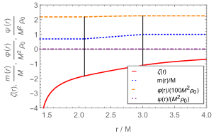
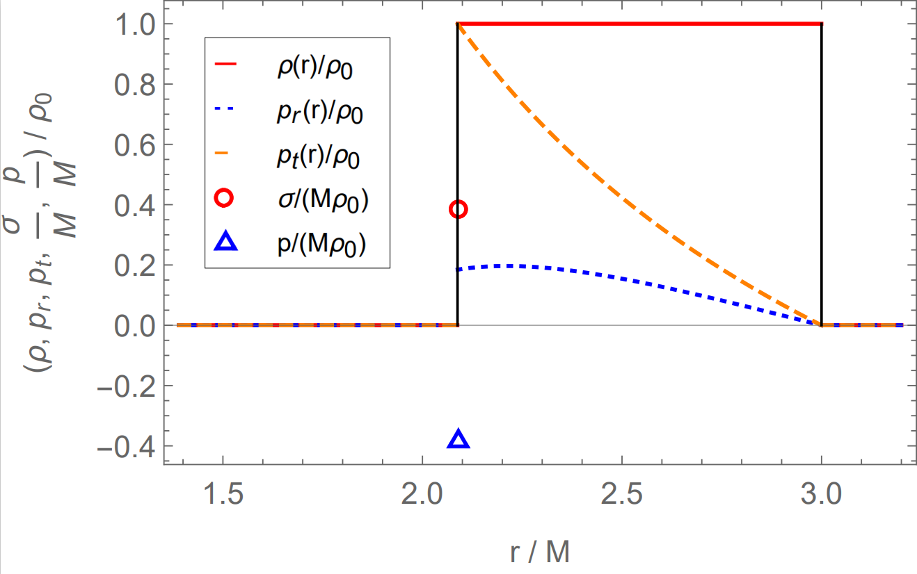
Figure 1: The full solution for the quasistar with a black hole. In the left panel it is plotted the metric fields $\zeta(r)$ and $m(r)$ in units of exterior spacetime mass $M$, and the scalar fields $\varphi(r)$ and $\psi(r)$ in units of $M^{2}\rho_{0}$, which is a dimensionless quantity, as functions of $r$, more precisely of $\frac{r}{M}$, and in the right panel it is plotted the matter fields $\rho(r)$, $p_{r}(r)$, $p_{t}(r)$, $\frac{\sigma}{M}$, and $\frac{p}{M}$, in units of $\rho_{0}$, as functions of $r$, more precisely of $\frac{r}{M}$, for the full solution, i.e., for $r_{h}<r<\infty$, where $r_{h}=2m$. Note that $\sigma$ and $p$ reveal the presence of a thin shell, a mild one, at $r_{\Sigma_{i}}$, whereas at $r_{\Sigma_{e}}$ the solution is smooth. The value chosen for $r_{\Sigma_{i}}$ is $r_{\Sigma_{i}}=2.09M$. Since $r_{h}$ is given by $r_{h}=\frac{2}{3}r_{\Sigma_{i}}$ one has $r_{h}=1.39M$. The value for $r_{\Sigma_{e}}$ is mandatorily $r_{\Sigma_{e}}=3M$. The values chosen for the other free parameters are $\psi_{0}=0$, $\rho_{0}=1$, and $M=1$, i.e., all is normalized to $M$. The NEC, WEC, and DEC, are satisfied for the full solution. See text for further details.

For the inferior border of the thick shell one has $r=r_{\Sigma_{i}}$, where to satisfy all the energy conditions $r_{\Sigma_{i}}$ is in the range given by Eq. (115) which can be put in terms of $m$ using Eq. (116). The line element can be taken from Eq. (93) evaluated at $r_{\Sigma_{i}}$, $\varphi$ has the value given in Eq. (VI.2.3), $\psi$ has the value given in Eq. (118), and there is a thin shell with $\sigma$ and $p$ given in Eqs. (119) and (120), respectively.

For the middle region, i.e., the thick shell solution, $r_{\Sigma_{i}}\leq r\leq r_{\Sigma_{e}}$, the line element is given in Eq. (VI.2.2) together with Eqs. (122) and (123). In addition, $\varphi$ is the function given in Eq. (VI.2.3), $\psi$ has the value given in Eq. (104), and the matter functions $\rho$, and $p_{r}$ and $p_{t}$, are given in Eqs. (105), and (VI.2.3), respectively.

For the superior border of the thick shell, one has $r=r_{\Sigma_{e}}$, and in terms of $M$ is given by Eq. (121). The line element is given in Eq. (107) evaluated at $r_{\Sigma_{e}}$, $\varphi$ has the value given in Eq. (126), $\psi$ has the value given in Eq. (125), and there is no thin shell, the matching is smooth.

For the exterior region, $r_{\Sigma_{e}}\leq r<\infty$, we have an exterior Schwarzschild spacetime given by the line element Eq. (107) with $M$ the spacetime mass, the field $\varphi$ is a constant given in Eq. (126), the field $\psi$ is a constant given in Eq. (125), and since it is vacuum there are no matter fields, see Eqs. (112) and (113).

The full solution is then given by all the equations cited above. The full solution is shown in Fig. 1, where plots of $\zeta(r)$, $m(r)$, $\varphi(r)$, $\psi(r)$, $\rho(r)$, $p_{r}(r)$, $p_{t}(r)$, $\sigma(r_{\Sigma_{i}})$, and $p(r_{\Sigma_{i}})$, are given as function of the radius $r$. The radius $r=r_{\Sigma_{i}}$ can be in the range $2.09M\leq r_{\Sigma_{i}}<3M$, where $3M=r_{\Sigma_{e}}$. For the plots we have chosen the free parameter $r_{\Sigma_{i}}$ as $r_{\Sigma_{i}}=2.09M$. The other free parameters left are chosen as $\psi_{0}=0$, $\rho_{0}=1$, and the rest is in terms of $M$, i.e., $M=1$. All other cases for $r_{\Sigma_{i}}$ different from $2.09M$ are similar. The only particular case worth of note is when $r_{\Sigma_{i}}=r_{\Sigma_{e}}=3M$, in which case the thick and thin shells disappear, there is no thick and no thin shell, and the solution is a Schwarzschild vacuum black hole with $M=m$.

VII Third application: A wormhole. Thin shell: Matching a matter interior to a Schwarzschild-AdS exterior

A third application for the use of junction conditions in the generalized hybrid metric-Palatini matter theory is to a wormhole solution. In the generalized hybrid metric-Palatini matter theory, as in theories of gravitation in which the gravitational sector is enlarged, there is the possibility that the energy conditions, in particular the NEC, for the matter sector are obeyed. In this manner, the wormhole is not exotic and the flaring out geometry necessary in every wormhole solution is supported by the higher-order curvature terms in the geometrical representation, or by the two fundamental scalar fields in the scalar-tensor representation. These terms can then be interpreted as a gravitational fluid, and in building such a wormhole one gets exoticity in the gravitational sector from a trade with exoticity in the matter sector.

We display here a wormhole solution using the scalar-tensor representation of the theory, knowing that in the geometrical representation we obtain the same expressions and quantities for the solution. The wormhole solution we want to work out is composed of three regions. The first region is the inside region containing matter, where the wormhole throat is situated. It has two branches that develop out from the throat as is usual in a wormhole solution. The second region, the middle region, is composed of a thin shell made of matter, actually, two similar shells, that join each interior branch to each exterior part. The third region, the exterior region, is a vacuum Schwarzschild-AdS region that extends up to infinity. This wormhole solution has the important feature that the NEC for the matter is verified for the entire spacetime. Its existence reinforces the believe that additional fundamental gravitational fields, such as the scalar fields used here, are behind the construction of wormholes that do not need exotic matter. Nonetheless, the engineering of these wormholes is hard to realize, even theoretically, and so these solutions are probably scant. This wormhole solution has been presented before rosa2018 . Here we refer briefly to the solution. We use consistently the nomenclature that we have been using for the metric fields, the scalar fields, and matter fields. The scalar tensor theory that we employ is one in which the potential for the scalar fields $\varphi(r)$ and $\psi(r)$ is $V(\varphi,\psi)$ of the form $V\left(\varphi,\psi\right)=V_{0}\left(\varphi-\psi\right)^{2}$, where $V_{0}$ is some free constant potential.

Let us start to present the interior region, $r_{0}\leq r\leq r_{\Sigma}$. This interior starts at the wormhole throat with radius $r_{0}$ and is composed of two symmetric branches, each branch is in the range $r_{0}\leq r\leq r_{\Sigma}$ and continues in a symmetric manner up to $r_{\Sigma}$ where the two branches are then connected to two independent exterior regions. The metric function $\zeta(r)$ is given by $\zeta(r)=\zeta_{0}$, where $\zeta_{0}$ is a free constant, and the other metric function $m(r)$ is given by $m(r)=\frac{r_{0}^{2}}{r}$, where $r_{0}$ is the radius of the wormhole throat, so that the line element is $ds^{2}=-e^{\zeta_{0}}dt^{2}+\left(1-\frac{r_{0}^{2}}{r^{2}}\right)^{-1}dr^{2}+r^{2}d\Omega^{2}$. The scalar field $\varphi(r)$ is given by $\varphi(r)=\psi_{0}-\frac{r_{0}^{2}}{V_{0}r^{4}}$, and the scalar field $\psi(r)$ is $\psi(r)=\psi_{0}$, where $\psi_{0}$ is a constant. The matter fields in this interior region, i.e., the energy density $\rho$, the radial pressure $p_{r}$, and the tangential pressure $p_{t}$ of the fluid, are given by $\rho=\frac{M^{6}}{4r^{6}}\left(\,{\mbox{\scriptsize 31}}\frac{r_{0}^{2}}{r^{2}}-{\mbox{\scriptsize 24}}\right)\rho_{0}$, $p_{r}=\frac{M^{6}}{4r^{6}}\left(\,{\mbox{\scriptsize 13}}\frac{r_{0}^{2}}{r^{2}}-{\mbox{\scriptsize 16}}\right)\rho_{0}$, and $p_{t}=\frac{M^{6}}{4r^{6}}\left(-{\mbox{\scriptsize 39}}\frac{r_{0}^{2}}{r^{2}}+{\mbox{\scriptsize 32}}\right)\rho_{0}$, where we have defined for convenience a standard density $\rho_{0}$ by $\rho_{0}\equiv\frac{r_{0}^{2}}{4\pi(-V_{0})M^{6}}$. Let us now present the solution at the thin shell, i.e., at $r=r_{\Sigma}$. There are two thin shells actually, each one at an $r_{\Sigma}$ that joins each exterior branch of the wormhole solution. At $r_{\Sigma}$ the metric function $\zeta(r)$ has the value $\zeta(r_{\Sigma})=\zeta_{0}$, the metric function $m(r)$ suffers a jump due to the fact that the shell has some energy-density, actually negative so that the mass decreases, the field $\varphi(r)$ is continuous and thus it has the value $\varphi(r_{\Sigma})=\psi_{0}-\frac{r_{0}^{2}}{V_{0}r_{\Sigma}^{4}}$, and the field $\psi(r)$ is continuous and thus it has the value $\psi(r_{\Sigma})=\psi_{0}$. There is matter in the thin shell, it has surface energy density given by $\frac{\sigma}{M}=\frac{M^{5}}{2r_{\Sigma}^{5}}\left(\,r_{\Sigma}k(r_{\Sigma})-4\right)\rho_{0}$, and surface pressure given by $\frac{p}{M}=\frac{M^{5}}{2r_{\Sigma}^{5}}\left(4+\frac{1}{2}\,r_{\Sigma}k(r_{\Sigma})\right)\rho_{0}$, where $k(r_{\Sigma})=\frac{r_{0}\zeta_{0}}{2r_{\Sigma}^{2}}\sqrt{1-\frac{r_{0}^{2}}{r_{\Sigma}^{2}}}+\frac{\frac{r_{0}^{2}}{r_{\Sigma}}-6M}{6r_{\Sigma}^{2}\sqrt{1-\frac{2M}{r_{\Sigma}}+\frac{r_{0}^{2}}{6r_{\Sigma}^{2}}}}$, and again $\rho_{0}=\frac{r_{0}^{2}}{4\pi(-V_{0})M^{6}}$. The NEC at the thin shell is obeyed if $\sigma+p>0$. One has to be careful in choosing $r_{\Sigma}$ since it has to be greater than the gravitational radius of the solution, otherwise there would be a horizon and the solution would be invalid. For this one has to bear in mind that the gravitational radius $r_{g}$ of an exterior Shwarzschild-AdS spacetime always obeys $r_{g}<2M$. Let us continue with the exterior region, $r_{\Sigma}\leq r<\infty$. The exterior region is composed of two symmetric parts each joining the interior region at a$r_{\Sigma}$. The metric function $\zeta(r)$ in the exterior is given by $e^{\zeta(r)}=\frac{1-\frac{2M}{r}-\Lambda r^{2}}{1-\frac{2M}{r_{\Sigma}}-\Lambda{r_{\Sigma}}^{2}}e^{\zeta_{0}}$, where $\Lambda$ is a cosmological constant given by $\Lambda=\frac{V_{0}(\varphi_{e}-\psi_{e})}{6}$, and the metric function $m(r)$ is $m(r)=2M+\Lambda r^{3}$, where $M$ is the exterior spacetime mass, so that the exterior line element is $ds^{2}=-\frac{1-\frac{2M}{r}-\Lambda r^{2}}{1-\frac{2M}{r_{\Sigma}}-\Lambda r_{\Sigma}^{2}}e^{\zeta_{0}}dt^{2}+\frac{dr^{2}}{1-\frac{2M}{r}-\Lambda r^{2}}+r^{2}d\Omega^{2}$, $r_{\Sigma}\leq r\leq\infty$. The scalar field $\varphi_{e}(r)$ is $\varphi_{e}(r)=\psi_{0}-\frac{r_{0}^{2}}{V_{0}{r_{\Sigma}}^{4}}$, and so is a constant, and the scalar field $\psi_{e}(r)$ is given by $\psi_{e}(r)=\psi_{0}$, also a constant. Thus, $\Lambda=-\frac{r_{0}^{2}}{6r_{\Sigma}^{4}}$. Then, $\Lambda$ is negative and the exterior spacetime is Schwarzschild-AdS. The matter fields in the exterior region are given by $\rho=0$, $p_{r}=0$, and $p_{t}=0$.

To have a definite solution we choose $r_{0}={\mbox{\scriptsize 2}}\sqrt{\frac{10}{11}}M$, $r_{\Sigma}=2M$, $\zeta_{0}=-10.96$, $\psi_{0}=1$, and $V_{0}=-42$. The choice for a negative $V_{0}$ is that it makes the quantity $\sigma+p$ positive and so the NEC is satisfied. Indeed, $\sigma=-0.0605\rho_{0}M$ and $p=0.0632\rho_{0}M$, so that $\sigma+p=0.0027\rho_{0}M$, is positive, and the matter in the shell obeys the NEC. $\Lambda$ is negative, it is $\Lambda=-0.03788$, thus the exterior is a Schwarzschild-AdS spacetime. We normalize all quantities to the spacetime mass $M$, which amounts to put $M=1$. The matter WEC does not hold on the shell but holds everywhere else. The matter NEC, which is the most important energy condition, is obeyed everywhere in conformity with our aim. This completes our full wormhole solution. Figure 2 displays the solution. For a full account of this wormhole solution see rosa2018 .

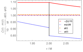
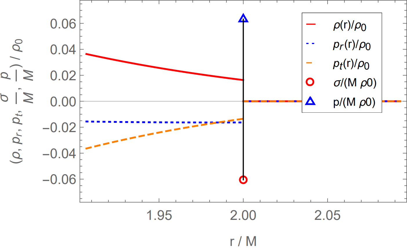
Figure 2: The full solution for the wormhole. In the left panel it is plotted the metric fields $\zeta(r)$ and $m(r)$ in units of exterior spacetime mass $M$, and the scalar fields $\varphi(r)$ and $\psi(r)$ which have no units, as functions of $r$, more precisely of $\frac{r}{M}$, and in the right panel it is plotted the matter fields $\rho(r)$, $p_{r}(r)$, $p_{t}(r)$, $\frac{\sigma}{M}$, and $\frac{p}{M}$, in units of $\rho_{0}$, as functions of $r$, more precisely of $\frac{r}{M}$, for the full solution, i.e., for $r_{0}<r<\infty$, where $r_{0}$ is the throat radius and there are two copies of $r$. Note that $\sigma$ and $p$ reveal the presence of thin shell at $r_{\Sigma}$. The value chosen for the throat radius $r_{0}$ is $r_{0}={\mbox{\scriptsize 2}}\sqrt{\frac{10}{11}}M$. The value chosen for $r_{\Sigma}$ is $r_{\Sigma}=2M$. The values chosen for the other free parameters are $\zeta_{0}=-10.96$, $\psi_{0}=1$, $V_{0}=-42$, and $M=1$, i.e., all is normalized to $M$. Since we have defined $\rho_{0}=\frac{r_{0}^{2}}{4\pi(-V_{0})M^{6}}$, one gets $\rho_{0}=0.00689$. $\Lambda=-\frac{r_{0}^{2}}{6r_{\Sigma}^{4}}$, so $\Lambda=-0.03788$. Also, $\frac{\sigma}{M}=-0.0605\rho_{0}$, and $\frac{p}{M}=0.0632\rho_{0}$. The matter NEC is satisfied for the full wormhole solution. See text for further details.

VIII Conclusions

The generalization from the general relativity action containing the Ricci scalar $R$ alone plus matter to generalized hybrid metric-Palatini gravity action containing in the geometric representation a function of the Ricci scalars $R$ and $\cal R$, and in the scalar-tensor representation a function of the Ricci scalar $R$ and two scalar fields $\psi$ and $\phi$, in which one can add matter fields to both, leads to new junction conditions in both representations. We have presented the junction conditions for the generalized hybrid metric-Palatini gravity, for both the geometrical and the scalar-tensor representation of the theory, in the cases of a thin shell junction and of a smooth matching.

In the geometrical representation of the generalized hybrid metric-Palatini gravity, in the case of a matching with a thin shell, the conformal relation between $R$ and $\mathcal{R}$, implies that the jump of the derivatives of $R$ and $\mathcal{R}$ do not contribute independently to the stress energy tensor of the shell. In fact, the two quantities must have a specific relation. It also follows that the normal derivative of the Ricci scalar being not continuous, gives rise to the existence of the matter thin shell. In the case of a smooth matching, we obtained that the trace of the extrinsic curvature and the Ricci scalar must be continuous, and also that the normal derivative of the Ricci scalar must be continuous. Moreover, given the conformal relation between $R$ and $\mathcal{R}$, it follows that the continuity of $R$ implies the continuity of $\mathcal{R}$.

In the scalar-tensor representation of the generalized hybrid metric-Palatini gravity, some interesting results also appeared which can be compared with the junction conditions for the Brans-Dicke theory. In the case of a matching with a thin shell, the trace of the extrinsic curvature must be continuous, on one hand emphasizing the relation between the geometrical and the scalar-tensor representation of the theory, on the other hand showing its difference to the Brans-Dicke theory where the trace of the extrinsic curvature does not need to be continuous. Moreover, since only the scalar field $\varphi$ is coupled to matter, only the derivative of $\varphi$ is allowed to be discontinuous in which case it contributes to the stress energy of the thin shell. In the case of a smooth matching, it turns out that the scalar fields and their normal derivatives must be continuous. As well, the trace of the extrinsic curvature must be continuous.

The importance and usefulness of these junction conditions is explicit, as it helped to find three different solutions, one for a spacetime with a thin shell as a simplified model of a star, other for a three-region spacetime with a thick shell as a simplified model of a quasistar, and yet another for a wormhole.

The use of the junction conditions allowed us to satisfy all the energy conditions for the star thin shell and the quasistar thick shell solutions, and to satisfy the matter NEC for the wormhole spacetime solution which generically is something very hard to achieve. These results point towards the physical relevance of the solutions obtained. Of course, to progress further with the physical meaningfulness of the solutions found, one has to perform a stability study to radial perturbations to start with, and then a full stability analysis.

It should be mentioned that, although the equivalence between the two representations, geometrical and scalar-tensor, can be unambiguous in some results, such as the continuity of the trace of the extrinsic curvature or the direct implication between the continuity of the scalar fields to the continuity of $R$ and $\mathcal{R}$, the equivalence of the remaining results is not so clear cut. For instance, in the second application of a quasistar which has a thick shell, although not obvious and not made explicitly, one can show that the transformation $f_{R}=\varphi$ yields the same expression in both representations, geometric and scalar-tensor, in what concerns the density and transverse pressure of the inner thin shell. Moreover, the relation between the derivatives of $R$ and $\mathcal{R}$ in the geometrical representation can also be found in the scalar tensor representation since a replacement $f_{\mathcal{R}}=\psi$ leads to the correct relation. We may then conclude that the junction conditions in both representations are indeed equivalent.

It has been also made clear that matched solutions in the generalized hybrid metric-Palatini gravity have more restrictions than matched solutions in general relativity. This means that matched solutions in general relativity may not necessarily be solutions in the generalized hybrid metric-Palatini gravity, a simple example of this fact is for self-gravitating thin shells of matter that in the generalized hybrid metric-Palatini gravity are constrained to have a specific radius $r_{\Sigma}=\frac{9M}{4}$, whereas in general relativity the shells can have any radius $r_{\Sigma}$ as long as $r_{\Sigma}$ is greater than the gravitational radius.

The restriction on the matching radius arises from the extra junction condition $\left[K\right]=0$, which does not exist in general relativity. This extra junction condition is common in metric theories of gravity where the Lagrangian has an arbitrary dependence on the metric Ricci scalar $R$, from which $f\left(R\right)$ and $f\left(R,T\right)$ are other known examples. To avoid the $\left[K\right]=0$ junction condition, one must recur to metric-affine theories of gravity, a well-known example being the case of the pure Palatini $f\left(\mathcal{R}\right)$ theory, and another possible example being the case of the Palatini $f\left(\mathcal{R},T\right)$ gravity theory.

Appendix A Explicit equation of Sec. II

We have derived the field equations of the generalized hybrid metric-Palatini gravity in the geometrical representation in terms of derivatives of the function $f\left(R,\mathcal{R}\right)$ in Sec. II. As shown in Eq. (II.1), these derivatives can be expanded in terms of derivatives of $R$ and $\mathcal{R}$. Since the complete expanded field equation is big, we opted to not write it there, we do it here. For that, we insert the set of equations given in Eq. (II.1) into the field equation given in Eq. (II.1), and obtain the fully extended field equation in the form

$$R_{ab}\left(f_{R}+f_{\mathcal{R}}\right)-\left(f_{RR}+f_{\mathcal{R}R}\right)\nabla_{a}\nabla_{b}-\left(f_{R\mathcal{R}}+f_{\mathcal{R}\mathcal{R}}\right)\nabla_{a}\nabla_{b}\mathcal{R}-\left(f_{RRR}+f_{R\mathcal{R}\mathcal{R}}\right)\partial_{a}R\partial_{b}R-\left(f_{R\mathcal{R}\mathcal{R}}+f_{\mathcal{R}\mathcal{R}\mathcal{R}}\right)\partial_{a}\mathcal{R}\partial_{b}\mathcal{R}-$$

$$-2\left(f_{R\mathcal{R}R}+f_{\mathcal{R}\mathcal{R}R}\right)\partial_{(a}R\partial_{b)}\mathcal{R}+g_{ab}\left[\left(f_{RR}-\frac{1}{2}f_{\mathcal{R}R}\right)\Box R+\left(f_{R\mathcal{R}}-\frac{1}{2}f_{\mathcal{R}\mathcal{R}}\right)\Box\mathcal{R}+\left(f_{RRR}-\frac{1}{2}f_{R\mathcal{R}\mathcal{R}}\right)\partial_{c}R\partial^{c}R+\right.$$

$$+\left.\left(f_{R\mathcal{R}\mathcal{R}}-\frac{1}{2}f_{\mathcal{R}\mathcal{R}\mathcal{R}}\right)\partial_{c}\mathcal{R}\partial^{c}\mathcal{R}+\left(2f_{R\mathcal{R}R}-f_{\mathcal{R}\mathcal{R}R}\right)\partial_{c}R\partial^{c}\mathcal{R}\right]+\frac{3}{2f_{\mathcal{R}}}\left(f_{\mathcal{R}R}^{2}\partial_{a}R\partial_{b}R+f_{\mathcal{R}\mathcal{R}}^{2}\partial_{a}\mathcal{R}\partial_{b}\mathcal{R}+2f_{\mathcal{R}R}f_{\mathcal{R}\mathcal{R}}\partial_{(a}R\partial_{b)}\mathcal{R}\right)-$$

$$-\frac{1}{3}g_{ab}f=8\pi T_{ab}.$$ (128)

Appendix B A more general theory for the star shell application of Sec. V

In Sec. V, in the first application of the junction conditions formalism in generalized hybrid metric-Palatini gravity, on a star thin shell matching an interior Minkowski spacetime to an exterior Schwarzschild spacetime, we have chosen a specific theory for $f\left(R,\mathcal{R}\right)$, namely, $f\left(R,\mathcal{R}\right)=R+\mathcal{R}+\frac{R\mathcal{R}}{R_{0}}$. Here we give a more general $f\left(R,\mathcal{R}\right)$ and find the matter properties for the thin shell in the geometrical representation.

We consider the following form of the function $f\left(R,\mathcal{R}\right)$,

$$f\left(R,\mathcal{R}\right)=g\left(R\right)+\mathcal{R}h\left(\dfrac{R}{R_{0}}\right)$$ (129)

where $g\left(R\right)$ and $h\left(\dfrac{R}{R_{0}}\right)$ are well behaved functions of their arguments, and $R_{0}$ is a constant with units of $R$. For this specific choice of the function $f$, we can write the derivatives $f_{R}$ and $f_{\mathcal{R}}$ as

$$f_{R}=g^{\prime}\left(R\right)+h^{\prime}\left(\bar{R}\right)\bar{\mathcal{R}},\quad\quad f_{\mathcal{R}}=h\left(\bar{R}\right),$$ (130)

and the second derivatives $f_{RR}$, $f_{R\mathcal{R}}$ and $f_{\mathcal{R}\mathcal{R}}$ as

$$f_{RR}=g^{\prime\prime}\left(R\right)+h^{\prime\prime}\left(\bar{R}\right)\frac{\bar{\mathcal{R}}}{R_{0}},\;f_{{\mathcal{R}}R}=h^{\prime}\left(\bar{R}\right)\frac{1}{R_{0}},\;f_{{\mathcal{R}}{\mathcal{R}}}=0\,,$$ (131)

where $\bar{\mathcal{R}}=\frac{\mathcal{R}}{R_{0}}$ and $\bar{R}=\frac{R}{R_{0}}$ are dimensionless variables. Eq. (3) becomes an equation for $\mathcal{R}_{ab}$ as a function of $R_{ab}$ and $R$ as

$$\mathcal{R}_{ab}= R_{ab}-\frac{1}{h\left(\bar{R}\right)}\left(\nabla_{a}\nabla_{b}+\frac{1}{2}g_{ab}\Box\right)h\left(\bar{R}\right)+$$ (132)

$$+\frac{3}{2h\left(\bar{R}\right)^{2}}\partial_{a}h\left(\bar{R}\right)\partial_{b}h\left(\bar{R}\right).$$

Notice that the specific choice of the function $f$ in Eq. (129) allows us to write $\mathcal{R}_{ab}$ as a function of $R_{ab}$ and $R$ only, implying that we can use Eq. (132) and its trace, and use Eqs. (129) and (130) to cancel the terms depending on $\mathcal{R}_{ab}$ and $\mathcal{R}$ in the field equation given in Eq. (II.1) and obtain an equation that only depends on the metric $g_{ab}$ and its derivatives. The simplification presented in Eq. (132) is not possible in general. Indeed, for a generic choice of the function $f$ for which $f_{\mathcal{R}}$ depends on $\mathcal{R}$, Eq. (3) becomes a partial differential equation for $\mathcal{R}$ and the problem is much more complicated.

Considering a Minkowski spacetime inside and a Schwarzschild spacetime outside, we can find the matter properties of the shell at $r_{\Sigma}$ for the theory given in Eq. (129). All we have worked out in Sec. V for the geometrical representation follows apart the the sixth junction condition of Eq. (III.1.1). The two components of Eq. (III.1.1) correspond to $S_{0}^{0}=-\sigma$ and $S_{\theta}^{\theta}=p$. Since, the the second junction condition in Eq. (III.1.1) is $\left[K\right]=0$, for a spherically symmetric thin shell one can write $\left[K_{0}^{0}\right]=-2\left[K_{\theta}^{\theta}\right]$, and so the sixth junction condition of Eq. (III.1.1) is given by the two independent components, namely, $\frac{\epsilon}{8\pi}\left[\left(f_{R}+f_{\mathcal{R}}\right)\left[K_{0}^{0}\right]-n^{c}\left[\partial_{c}R\right]\left(f_{RR}-\frac{f_{\mathcal{R}R}^{2}}{f_{\mathcal{R}\mathcal{R}}}\right)\right]=\sigma$ and $\frac{\epsilon}{8\pi}\left[n^{c}\left[\partial_{c}R\right]\left(f_{RR}-\frac{f_{\mathcal{R}R}^{2}}{f_{\mathcal{R}\mathcal{R}}}\right)+\frac{1}{2}\left(f_{R}+f_{\mathcal{R}}\right)\left[K_{0}^{0}\right]\right]=p$, see Eqs. (62) and (63). From these two equations we obtain for our specific case, i.e., from Eqs. (129), (130), and (131), and using $\epsilon=1$ since $n^{a}$ points in the radial direction and thus is a spacelike vector,

$$\sigma=\frac{1}{8\pi}\left\{\left[g^{\prime}\left(R\right)+h\left(\bar{R}\right)\right]\frac{16}{27M}\right\}\,,$$ (133)

$$p=\frac{1}{16\pi}\left\{\left[g^{\prime}\left(R\right)+h\left(\bar{R}\right)\right]\frac{16}{27M}\right\}\,,$$ (134)

where we have used that since $\left[K_{0}^{0}\right]=\frac{M}{r_{\Sigma}^{2}}\frac{1}{\sqrt{1-\frac{2M}{r_{\Sigma}}}}$ and $r_{\Sigma}=\frac{9}{4}M$, see Eq. (70), one has $\left[K_{0}^{0}\right]|_{r_{\Sigma}}=\frac{16}{27M}$. Thus, from these equations, one has $\sigma=2p$, which is the expected result as the matching is being performed at the Buchdahl radius, as stated before.

To have a direct comparison of the geometrical representation results with the scalar-tensor representation results one has to specify form for $f\left(R,\mathcal{R}\right)$. It is at this point that we choose $g\left(R\right)$ and $h\left(\bar{R}\right)$ as

$$g\left(R\right)=R,\qquad h\left(\frac{R}{R_{0}}\right)=1+\frac{R}{R_{0}},$$ (135)

for which the function $f\left(R,\mathcal{R}\right)$ is

$$f\left(R,\mathcal{R}\right)=R+\mathcal{R}+\frac{R\mathcal{R}}{R_{0}}\,,$$ (136)

the one given in Eq. (67). For this particular form of the function $f$, one has $g^{\prime}\left(R\right)=1$ and $h\left(\bar{R}\right)=1$, and the first and second derivatives $f_{R}$, $f_{\mathcal{R}}$, $f_{RR}$, $f_{\mathcal{R}\mathcal{R}}$ and $f_{R\mathcal{R}}$ become $f_{R}=1+\bar{\mathcal{R}}$, $f_{\mathcal{R}}=1+\bar{R}$, $f_{RR}=f_{\mathcal{R}\mathcal{R}}=0$, $f_{R\mathcal{R}}=\frac{1}{R_{0}}$. Then, Eqs. (133) and  (134) give $\sigma=\frac{4}{27\pi M}$ and $p=\frac{2}{27\pi M}$, respectively, which are Eqs. (71) and (72) of Sec. V.

Appendix C Solution for the radial and tangential pressures of the thick shell of Sec. VI

In Sec. VI we have seen that the matter energy density $\rho$ of the thick shell is a constant $\rho=\rho_{0}$. Before performing the matching, the radial and tangential pressures on the thick shell presented succinctly in Eq. (106) are here displayed explicitly. They are

$$p_{r}\left(r\right)=\frac{1}{64\pi r_{\Sigma_{e}}\left(7M-3r_{\Sigma_{e}}\right)r^{\frac{1}{2}\left(5+\beta\right)}}\left\{\left(r_{\Sigma_{e}}\right)^{2}\left[32\pi r^{\frac{5+\beta}{2}}\left(1+\beta\right)\rho_{0}+3\left(7+\beta^{2}\right)\varphi_{1}-3r^{\beta}\left(\beta^{2}+6\beta-7\right)\varphi_{2}\right]\right.$$

$$+14M^{2}\Big{[}\left(3+\beta^{2}\right)\varphi_{1}-r^{\beta}\left(\beta^{2}+6\beta-3\right)\varphi_{2}\Big{]}-Mr_{\Sigma_{e}}\left[32\pi r^{\frac{5+\beta}{2}}\left(3+2\beta\right)\rho_{0}+\left(67+13\beta^{2}\right)\varphi_{1}\right.$$

$$\left.\left.-r^{\beta}\left(13\beta^{2}+78\beta-67\right)\varphi_{2}\right.\right.\Big{]}\Big{\}}\,,$$

$$p_{t}\left(r\right)=-\frac{1}{64\pi r_{\Sigma_{e}}\left(7M-3r_{\Sigma_{e}}\right)r^{\frac{1}{2}\left(5+\beta\right)}}\left[8\pi r^{r_{\Sigma_{e}}\frac{5+\beta}{2}}\left(\beta^{2}+2\beta+13\right)\rho_{0}+2\left(7M-3r_{\Sigma_{e}}\right)\left(3+\beta^{2}\right)\varphi_{1}\right.$$

$$\left.+6r^{\beta}\left(7M-3r_{\Sigma_{e}}\right)\left(\beta-1\right)^{2}\varphi_{2}\right]\,,\quad\quad\quad r_{\Sigma_{i}}\leq r\leq r_{\Sigma_{e}}\,,$$ (137)

where $\beta=\sqrt{\frac{r_{\Sigma_{e}}+6M}{r_{\Sigma_{e}}-2M}}$, $\rho_{0}$ is the constant energy density of the thick shell, $M$ is the exterior spacetime mass, $r_{\Sigma_{e}}$ is the exterior radius of the thick shell, and $\varphi_{1}$ and $\varphi_{2}$ are constants of integration that appear is the solution for $\varphi(r)$, see Eq. (VI.2.3). For the values obtained using the junction conditions, i.e., $r_{\Sigma_{e}}=3M$, $\varphi_{1}=54\pi M^{2}\rho_{0}$, and $\varphi_{2}=40\pi M^{2}\rho_{0}$, one finds $p_{r}\left(r\right)=\frac{1}{2}\left(-3-\frac{27M^{4}}{r^{4}}+\frac{10M}{r}\right)\rho_{0}$ and $p_{t}\left(r\right)=\frac{1}{4}\left(-7+\frac{27M^{4}}{r^{4}}+\frac{20M}{r}\right)\rho_{0}$, which are the expressions given in Eq. (VI.2.3).

The unprocessed solution for the middle region, i.e., the thick shell solution without taking into account the junction conditions, is visualized in Fig. C1, where all the fields are plotted.

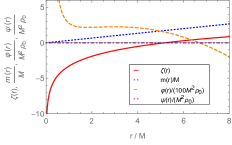
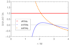
Figure C1: The unprocessed solution for the thick shell. In the left panel it is plotted the metric fields $\zeta(r)$ and $m(r)$ in units of exterior spacetime mass $M$, and the scalar fields $\varphi(r)$ and $\psi(r)$ in units of $M^{2}\rho_{0}$, which is a dimensionless quantity, as functions of $r$, more precisely of $\frac{r}{M}$, and in the right panel it is plotted the matter fields $\rho(r)$, $p_{r}(r)$, $p_{t}(r)$, in units of $\rho_{0}$, as functions of $r$, more precisely of $\frac{r}{M}$, valid for $0\leq r<\infty$. The values chosen for the free parameters are $\psi_{0}=0$, $\rho_{0}=1$, and $M=1$, i.e., all is normalized to $M$.

References

- (1) G. Darmois, “Les équations de la gravitation einsteinienne”, Memorial des Sciences Mathématiques, 25, 1 (1927).
- (2) A. Lichnerowicz, Théories Relativistes de la Gravitation et de l’Électromagnétisme (Masson, Paris 1955).
- (3) K. Lake, “Revisiting the Darmois and Lichnerowicz junction conditions”, Gen. Relativ. Gravit. 49, 134 (2017); arXiv:1705.01090 [gr-qc].
- (4) K. Lanczos, “Bemerkungen zur de Sitterschen Welt”, Physikalische Zeitschrift 23, 539, (1922).
- (5) N. Sen, “Über die Grenzbedingungen des Schwerefeldes an Unstetigkeitsflächen”, Annalen der Physik 378, 365 (1924).
- (6) K. Lanczos, “Flächenhafte Verteiliung der Materie in der Einsteinschen Gravitationstheorie”, Annalen der Physik 379, 518, (1924).
- (7) W. Israel, “Singular hypersurfaces and thin shells in general relativity”, Nuovo Cim. B 44, 1 (1966).
- (8) A. Papapetrou and A. Hamoui, “Couches simples de matière en relativité générale”, Annales de l’Institute Henri Poincaré A 9, 179 (1968).
- (9) A. H. Taub, “Space-times with distribution valued curvature tensors”, Journal of Mathematical Physics 21, 1423 (1980).
- (10) W. Arkuszewski, W. Kopczyński, and V. N. Ponomariev, “Matching conditions in the Einstein-Cartan theory of gravitation”, Commun. Math. Phys. 45, 183 (1975).
- (11) K. G. Suffern, “Singular hypersurfaces in the Brans-Dicke theory of gravity”, Journal of Physics A: Mathematical and General 15, 1599 (1982).
- (12) C. Barrabès and G. F. Bressange, “Singular hypersurfaces in scalar-tensor theories of gravity”, Classical Quantum Gravity 14, 805 (1997); arXiv:gr-qc/9701026.
- (13) S. C. Davis, “Generalized Israel junction conditions for a Gauss-Bonnet brane world”, Phys. Rev. D 67, 024030 (2003); arXiv:hep-th/0208205.
- (14) J. M. M. Senovilla, “Gravitational double layers”, Classical Quantum Gravity 31, 072002 (2014); arXiv:1402.1139 [gr-qc].
- (15) V. A. Berezin, V. I. Dokuchaev, Yu. N. Eroshenko, and A. L. Smirnov, “Double layer from least action principle”, Classical and Quantum Gravity 38, 045014 (2021); arXiv:2008.01813 [gr-qc].
- (16) N. Deruelle, M. Sasaki, and Y. Sendouda, “Junction conditions in theories of gravity”, Prog. Theor. Phys. 119, 237 (2008); arXiv:0711.1150 [gr-qc].
- (17) J. M. M. Senovilla, “Junction conditions for -gravity and their consequences”, Phys. Rev. D 88, 064015 (2013); arXiv:1303.1408 [gr-qc].
- (18) S. Vignolo, R. Cianci, and S. Carloni, “On the junction conditions in -gravity with torsion”, Class. Quant. Grav. 35, 095014 (2018); arXiv:1801.08344 [gr-qc].
- (19) G. J. Olmo and D. Rubiera-Garcia, “Junction conditions in Palatini gravity”, Classical Quantum Gravity 37, 215002 (2020); arXiv:2007.04065 [gr-qc].
- (20) J. L. Rosa, “Junction conditions and thin shells in perfect-fluid gravity”, Phys. Rev. D 103, 104069 (2021); arXiv:2103.11698 [gr-qc].
- (21) J. P. S. Lemos and V. T. Zanchin, “Plethora of relativistic charged spheres: The full spectrum of Guilfoyle’s static, electrically charged spherical solutions”, Phys. Rev. D 95, 104040 (2017); arXiv:2007.04065 [gr-qc].
- (22) J. L. Rosa and P. Piçarra, “Existence and stability of relativistic fluid spheres supported by thin shells”, Phys. Rev. D 102, 064009 (2020); arXiv:2006.09854 [gr-qc].
- (23) F. Fayos, J. M. M. Senovilla, and R. Torres, “General matching of two spherically symmetric spacetimes”, Phys. Rev. D 54, 4862 (1996).
- (24) D. L. F. G. Silva, Gravitational Collapse and Black Holes (MSc Thesis, Instituto Superior Técnico, 2020).
- (25) J. Frauendiener, C Hoenselaers, and W. Konrad, “A shell around a black hole”, Classical Quantum Gravity 7, 585 (1990).
- (26) G. A. S. Dias and J. P. S. Lemos, “Thin-shell wormholes in -dimensional general relativity: Solutions, properties, and stability”, Phys. Rev. D 82, 084023 (2010); arXiv:1008.3376 [gr-qc].
- (27) J. C. Feng, J. P. S. Lemos, and R. A. Matzner, “Self-collision of a portal wormhole”, Physical Review D 103, 124037 (2021); arXiv:2105.03433 [gr-qc].
- (28) P. Luz and S. Carloni, “Static compact objects in Einstein-Cartan theory”, Phys. Rev. D 100, 08403 (2019); arXiv:1907.11489 [gr-qc].
- (29) S. V. Sushkov and S. M. Kozyrev, “Applications in Brans-Dicke by composite vacuum Brans-Dicke wormholes”, Phys. Rev. D, 84, 124026 (2011); arXiv:1109.2273 [gr-qc].
- (30) M. A. Ramirez, “Vacuum thin shells in Einstein–Gauss-Bonnet brane-world cosmology”, Classical Quantum Gravity 35, 085004 (2018); arXiv:1709.05577 [gr-qc].
- (31) E. F. Eiroa and G. Figueroa-Aguirre, “Thin-shell wormholes with a double layer in quadratic gravity”, Phys. Rev. D 94, 044016 (2016); arXiv:1605.07089 [gr-qc].
- (32) E. F. Eiroa and G. Figueroa-Aguirre, “Thin shells in gravity with non-constant scalar curvature”, Eur. Phys. J. Plus 135, 774 (2020); arXiv:2005.10694 [gr-qc].
- (33) K. A. Bronnikov “Spherically symmetric black holes and wormholes in hybrid metric-Palatini gravity”, Gravitation and Cosmology 25, 331 (2019); arXiv:1908.02012 [gr-qc].
- (34) S. K. Maurya, A. Errehymy, D. Deb, F. Tello-Ortiz, and M. Daoud, “Study of anisotropic strange stars in gravity: An embedding approach under the simplest linear functional of the matter-geometry coupling”, Phys. Rev. D 100, 044014 (2019); arXiv:1907.10149 [gr-qc].
- (35) N. Tamanini and C. G. Boehmer, “Generalized hybrid metric-Palatini gravity”, Phys. Rev. D 87, 084031 (2013); arXiv:1302.2355 [gr-qc].
- (36) J. L. Rosa, S. Carloni, J. P. S. Lemos, and F. S. N. Lobo, “Cosmological solutions in generalized hybrid metric-Palatini gravity”, Phys. Rev. D 95, 124035 (2017); arXiv:1703.03335 [gr-qc].
- (37) J. L. Rosa, J. P. S. Lemos, and F. S. N. Lobo, “Wormholes in generalized hybrid metric-Palatini gravity obeying the matter null energy condition everywhere”, Phys. Rev. D 98, 064054 (2018); arXiv: 1808.08975 [gr-qc].
- (38) F. Bombacigno, F. Moretti, and G. Montani, “Scalar modes in extended hybrid metric-Palatini gravity: weak field phenomenology”, Phys. Rev. D 100, 124036 (2019); arXiv:1907.11949 [gr-qc].
- (39) J. L. Rosa, S. Carloni, and J. P. S. Lemos, “The cosmological phase space of generalized hybrid metric-Palatini theories of gravity”, Phys. Rev. D 101, 104056 (2020); arXiv:1908.07778 [gr-qc].
- (40) J. L. Rosa, J. P. S. Lemos, and F. S. N. Lobo, “Stability of Kerr black holes in generalized hybrid metric-Palatini gravity”, Phys. Rev. D 101, 044055 (2020); arXiv:2003.00090 [gr-qc].
- (41) H. M. R. da Silva, T. Harko, F. S. N. Lobo, and J. L. Rosa, “Cosmic strings in generalized hybrid metric-Palatini gravity”, Phys. Rev. D 101, 124050 (2020); arXiv:2104.12126 [gr-qc].
- (42) J. L. Rosa, D. A. Ferreira, D. Bazeia, and F. S. N. Lobo, “Thick brane structures in generalized hybrid metric-Palatini gravity”, European Physical Journal C 81, 20 (2021); arXiv:2010.10074 [gr-qc].
- (43) J. L. Rosa, F. S. N. Lobo, and D. Rubiera-Garcia, “Sudden singularities in generalized hybrid metric-Palatini cosmologies”, J. Cosmol. Astropart. Phys JCAP 07 (2021) 009 ; arXiv:2103.02580 [gr-qc].
- (44) J. L. Rosa, F. S. N. Lobo, and G. J. Olmo, “Weak-field regime of the generalized hybrid metric-Palatini gravity” (2021); arXiv:2104.10890 [gr-qc].
- (45) J. L. Rosa, “Double gravitational layer traversable wormholes in hybrid metric-Palatini gravity”, Phys. Rev. D 104, 064002 (2021); arXiv:2107.14225 [gr-qc].