RIS-Assisted Receive Quadrature Space-Shift Keying: A New Paradigm and Performance Analysis

Abstract

RIS represent a promising candidate for sixth-generation (6G) wireless networks, as the RIS technology provides a new solution to control the propagation channel in order to improve the efficiency of a wireless link through enhancing the received signal power. In this paper, we propose -assisted receive quadrature space-shift keying (-RQSSK), which enhances the spectral efficiency of an RIS-based index modulation (IM) system by using the real and imaginary dimensions independently for the purpose of IM. Therefore, the error rate performance of the system is improved as all RIS elements reflect the incident transmit signal toward both selected receive antennas. At the receiver, a low-complexity but effective greedy detector (GD) can be employed which determines the maximum energy per dimension at the receive antennas. A max-min optimization problem is defined to maximize the received signal-to-noise ratio (SNR) components at both selected receive antennas; an analytical solution is provided based on Lagrange duality. In particular, the multi-variable optimization problem is shown to reduce to the solution of a single-variable equation, which results in a very simple design procedure. In addition, we investigate the average bit error probability (ABEP) of the proposed -RQSSK system and derive a closed-form approximate upper bound on the ABEP. We also provide extensive numerical simulations to validate our derivations. Numerical results show that the proposed -RQSSK scheme substantially outperforms recent prominent benchmark schemes. This enhancement considerably increases with an increasing number of receive antennas.

I Introduction

In wireless communications, the recent emergence of many new applications and services necessitates the advent of new technologies in order to support a very large number of mobile devices as well as massive machine-type communications. To this end, several new technologies have emerged in fifth-generation (5G) wireless networks, including massive (mMIMO), millimeter-wave (mmWave) communications and small cells. However, these technologies intensify the use of energy and the hardware cost, which makes practical targets difficult to reach. In addition, 5G appears to be insufficient to meet the forthcoming requirements of next-generation wireless communications, as 5G technologies only target the endpoints of a wireless link, and make no attempt to influence or design the wireless environment which plays a major role in degrading the link’s efficiency. Therefore, controlling the propagation channel has received growing attention in the last few years, and accordingly the technology of RISs is a potentially key approach for 6G wireless networks [1, 2, 3, 4, 5, 6, 7, 8].

RIS are electromagnetic surfaces that can be electronically controlled by the network operator. An RIS consists of an array of small, low-cost and nearly-passive scattering elements that can induce a pre-designed phase shift in the incident wave. Thus RISs can modify in an energy-efficient manner the scattering, reflection and refraction of the environment with a view to enhancing the efficiency of a wireless network.

In [9], an RIS was deployed to enhance a communication system in two different scenarios: an RIS-based single-input single-output (SISO) scheme, where an RIS acts as a reflector and helps to perform beamforming, and an RIS-access point (RIS-AP) scheme, in which an RIS is utilized as a transmitter (access point) to convey the information bits through the phases of the RIS elements. For each scheme, the symbol error probability (SEP) of the system was analyzed and an enormous benefit was demonstrated compared to the conventional wireless system without the RIS. An RIS was deployed in a multiple-input single-output (MISO) system in [10], where the RIS, in addition to beamforming, also conveys its own information data via reflection pattern modulation (RPM). An alternating optimization (AO) algorithm was used to optimize active and passive beamforming, respectively, at the transmitter and RIS, in order to maximize the signal power at the receiver. A multi-user RIS-based downlink communication system was considered in [11] and an optimization problem was defined to maximize the energy efficiency of the system; again, an AO algorithm was applied to optimize both the transmit power allocation and the phases of the RIS elements. In [12], the projected gradient method (PGM) was used to maximize the achievable rate in an RIS-based MIMO communication system.

On the other hand, SM, or more generally IM, has been widely under investigation in the last decade due to its inherent energy efficiency. Massive connectivity results in enormously increasing energy consumption, while in IM part of the information is conveyed by the indices of the available resources, e.g. transmit or receive antennas, frequency-domain subcarriers, etc., such that only a subset of the energy-consuming resources are activated at any time; this characterizes IM as an energy-efficient solution. Therefore, IM has been recognized as another promising technology in 6G systems, thus motivating researchers to develop RIS-based IM systems. In particular, - (RIS-SSK) and - (RIS-SM) systems were introduced in [13], where indices of receive antennas can be considered to realize IM, while an RIS was deployed at the transmitter as an access point. The bit error rate (BER) performance of these systems was investigated and compared to that of the RIS-AP scheme in [9]. Inspired by [13], the authors in [14] analyzed the BER performance of a MISO RIS-assisted SSK system where the index of the transmit antenna conveyed the information. In [15], a new RIS-based SM paradigm was proposed in which the indices of both the transmit and receive antennas are selected in order to convey information; hence, the spectral efficiency is increased at the expense of a higher receiver complexity. Inspired by quadrature spatial modulation (QSM) proposed in [16], which implements SM independently on the real (in-phase) and imaginary (quadrature) dimensions, RIS-aided receive quadrature reflecting modulation (RIS-RQRM) was proposed in [17]. In this approach, the RIS elements are divided into two equal groups each of which independently performs SM. Although this technique doubles the spectral efficiency, it suffers from a degraded BER performance compared to RIS-SM. The concept of SM has been extended to GSM in [18] and [19] to increase the spectral efficiency of the RIS-based wireless system. However, in these schemes, the RIS elements are divided into a number of groups in order to maintain beamforming toward multiple selected receive antennas, which yields a reduction in the received signal power. Another RIS-based SSK scheme (SSK at the transmitter side, similar to [14]) was proposed in [20]. In this scheme, however, the RIS was assumed to have no knowledge regarding the transmit data, and therefore an optimization problem was defined to maximize the minimum squared channel-imprinted Euclidean distance at the receiver. The authors also proposed an extension to the scheme such that the RIS, in addition to reflecting the incident SSK signal, also transmits its own information via an Alamouti STBC. In [21] and [22], the concept of IM has been applied within the RIS entity, in which the RIS elements are divided into two groups so that IM can be implemented on these groups in order to transmit environmental data to the receiver, similar to the reflection pattern modulation (RPM) scheme of [10].

However, in all of the aforementioned studies, each group of RIS elements separately targets one receive or transmit antenna for the purpose of implementing SM. Despite the advantages of SM, the spectral efficiency of SM needs to be improved, and this can be performed by introducing other variants of SM such as quadrature spatial modulation (QSM) or GSM, which require two or more antennas to be activated. The proposed solutions so far, however, cut down the effective number of RIS elements. Hence, the spectral efficiency increases only at the cost of a reduction in the received signal power.

Against this background, in this paper we introduce a new paradigm for RIS-based IM in which the information is conveyed through the indices of two selected receive antennas. The resulting approach has the property that all RIS elements can independently perform beamforming onto the two selected receive antennas. The contributions of this paper are as follows:

• Inspired by QSM, we propose a novel RIS-assisted IM scheme, namely -RQSSK, in which all RIS elements simultaneously maximize the SNR of the in-phase and quadrature components of the received signal at the selected antennas. That is, the SNR associated to the real part of the signal at one antenna and the SNR associated to the imaginary part of the signal at the second antenna are maximized in order to be detectable by a simple GD. Therefore, the spectral efficiency is increased compared to conventional SSK, without significant additional complexity or cost.

• We propose a max-min optimization problem in order to maximize the two relevant SNR components. Since this problem is non-convex, we determine its dual problem, which is convex and admits an analytical solution. Specifically, the joint optimization of the RIS phase shifts reduces to solving a single-variable equation in order to determine each optimal RIS phase shift. We also show that with a large number of RIS elements the solution of this equation tends to a constant value, thus providing a very simple design procedure to control the phase of the RIS elements.

• We analyze the ABEP of the -RQSSK system. We also use approximations in order to derive a closed-form approximate ABEP which is tight in the SNR range of interest for a large number of RIS elements.

• Finally, we investigate the BER performance of the -RQSSK system through numerical simulations and compare the results with those of the most prominent recently proposed schemes. The results show that the proposed -RQSSK system significantly outperforms these benchmark schemes, and that the performance enhancement improves with an increasing number of receive antennas.

The rest of this paper is organized as follows. We describe the -RQSSK system model in Section II. In Section III, we formulate the optimization problem and investigate its analytical solution. The ABEP performance of the proposed -RQSSK system with and without polarity bits is analyzed in Section IV. Numerical simulations and comparisons with the benchmark schemes are provided in Section V. Finally, Section VI concludes this paper.

Notation: Boldface lower-case letters denote column vectors, and boldface upper-case letters denote matrices. $\mathbf{v}>0$ (resp., $\mathbf{v}\geq 0$) indicates that all elements in vector $\mathbf{v}$ are positive (resp., non-negative). $\mathbf{u}\odot\mathbf{v}$ represents the element-wise product of two equal-sized vectors $\mathbf{u}$ and $\mathbf{v}$. The superscripts $\left(\cdot\right)^{T}$ and $\left(\cdot\right)^{H}$ denote transpose and Hermitian transpose, respectively. $\left(\cdot\right)^{\mathcal{R}}$ and $\left(\cdot\right)^{\mathcal{I}}$ denote the real and imaginary components of a scalar/vector, respectively. $\mathsf{\mathbb{E}}\left\{\cdot\right\}$ and $\mathbb{V}\left\{\cdot\right\}$, respectively, denote the expectation and variance operator. $\mathcal{N}\left(\mu,\sigma^{2}\right)$ (resp., $\mathcal{CN}\left(\mu,\sigma^{2}\right)$) represents the normal (resp., complex normal) distribution with mean $\mu$ and variance $\sigma^{2}$. $\chi_{d}^{2}$ and $\chi_{d}^{2}\left(\lambda\right)$ denote central and non-central chi-square distributions, respectively, with $d$ degrees of freedom and non-centrality parameter $\lambda$. Finally, the set of complex matrices of size $m\times n$ is denoted by $\mathbb{C}^{m\times n}$.

II System Model

The proposed -assisted receive quadrature space-shift keying (-RQSSK) system is illustrated in Fig. 1. In this scenario, we consider an RIS-AP scheme in which the RIS forms part of the transmitter and it reflects the incident wave emitted from a single RF source which is located in the vicinity of the RIS such that the path loss of the link between the RIS and the RF source is negligible. The RIS is equipped with $N$ reflecting elements whose phases are controlled by the transmitter through the RIS controller. We assume that the receiver, which is equipped with $N_{r}$ antennas, can only receive the signal reflected from the RIS elements. The concept of RIS-AP was first introduced in [1] and [9]; later, in [13], this model was extended to cover RIS-aided wireless communication systems using IM techniques.

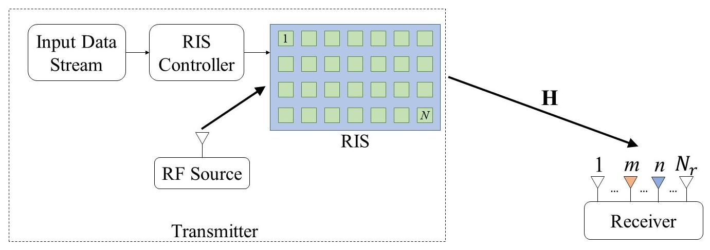
Figure 1: A schematic representation of the proposed -RQSSK system.

The baseband receive signal at receive antenna $l$ is given by

$$y_{l}=\sqrt{E_{s}}\mathbf{h}_{l}\boldsymbol{\theta}+n_{l},$$ (1)

where $\mathbf{h}_{l}=\left[h_{l,1},h_{l,2},\dots,h_{l,N}\right]\in\mathbb{C}^{1\times N}$ is the $l$-th row of $\mathbf{H}\in\mathbb{C}^{N_{r}\times N}$, which is the channel matrix of the link between the RIS and the receiver whose elements are i.i.d and distributed according to $\mathcal{CN}\left(0,1\right)$. $\boldsymbol{\theta}\in\mathbb{C}^{N\times 1}$ is the vector that consists of the reflection coefficients of the RIS elements, such that $\left|\theta_{i}\right|=1$ for $i=1,2,\dots,N$ (here we assume lossless reflection from the RIS). $E_{s}$ is the transmitted energy from the RF source per IM symbol, and $n_{l}\in\mathbb{C}$ is the additive white Gaussian noise at the $l$-th receive antenna that is distributed according to $\mathcal{CN}\left(0,N_{0}\right)$. Hence, the SNR is equal to $E_{s}/N_{0}$.

In the proposed RIS-RQSSK system, the input data bit stream is split into blocks of $R=2\left(\log_{2}N_{r}+1\right)$ bits; one packet of $\log_{2}N_{r}+1$ bits is mapped to an in-phase (real) signal, while the other packet of $\log_{2}N_{r}+1$ bits is mapped to a quadrature (imaginary) signal. In each of the two constituent packets of $(\log_{2}N_{r}+1)$ bits, the first $\log_{2}N_{r}$ bits are mapped to one receive antenna index and the final bit determines the corresponding polarity. In fact, the transmitted data bits determine the indices of two selected receive antennas. Unlike RIS-SSK [13], where the transmitter aims to maximize the SNR at one specific receive antenna, in the proposed scheme the transmitter independently selects two receive antennas. That is, the transmitter aims to simultaneously maximize the SNR of the real part of the signal at the first selected receive antenna, while also maximizing the SNR of the imaginary part of the signal at the second selected receive antenna. Recalling RSM techniques within MIMO systems, receive antenna selection can be performed via implementing a precoding matrix along with a transmit vector at the transmitter; however, in the RIS-AP scheme, where the transmitter (RF source) is equipped with only one antenna, passive beamforming via adjusting the phase of the RIS elements conducts the antenna selection task. In the next section, we will show in detail how the RIS reflection coefficient vector $\boldsymbol{\theta}$ is optimized to perform the so-called passive beamforming. Note that in this work, we assume that the transmitter has perfect knowledge of the channel state information (CSI) that is needed in order to calculate the optimal RIS phase shifts.

Suppose that $m$ and $n$ are the selected antenna indices for the real and imaginary parts, respectively. After expanding (1) for selected antennas $m$ and $n$, and separating the real and imaginary parts, we have

$$y_{m}^{\mathcal{R}} =\sqrt{E_{s}}\left[\mathbf{h}_{m}^{\mathcal{R}}\boldsymbol{\theta}^{\mathcal{R}}-\mathbf{h}_{m}^{\mathcal{I}}\boldsymbol{\theta}^{\mathcal{I}}\right]+n_{m}^{\mathcal{R}},$$ (2)

$$y_{n}^{\mathcal{I}} =\sqrt{E_{s}}\left[\mathbf{h}_{n}^{\mathcal{R}}\boldsymbol{\theta}^{\mathcal{I}}+\mathbf{h}_{n}^{\mathcal{I}}\boldsymbol{\theta}^{\mathcal{R}}\right]+n_{n}^{\mathcal{I}}.$$ (3)

The receive signal components (2) and (3) suggest that $\boldsymbol{\theta}$ needs to be optimized in order to maximize the relevant SNRs. After this SNR maximization has been performed, a simple but effective greedy detector (GD) can be employed to detect the selected receive antennas without the need for any knowledge of the CSI at the receiver. Then, the GD operates via

$$\hat{m} =\arg\max_{m\in\{1,2,\dots,N_{r}\}}\left\{\left(y_{m}^{\mathcal{R}}\right)^{2}\right\},$$ (4)

$$\hat{n} =\arg\max_{n\in\{1,2,\dots,N_{r}\}}\left\{\left(y_{n}^{\mathcal{I}}\right)^{2}\right\}.$$ (5)

That is, the GD estimates the antenna indices by independently searching over the instantaneous energy of the real and imaginary parts of the signal at the receive antennas and choosing the one with highest energy in each case (note that we may have $\hat{m}=\hat{n}$). After this, the polarity bits can be detected simply by testing the sign of each of the values $y_{\hat{m}}^{\mathcal{R}}$ and $y_{\hat{n}}^{\mathcal{I}}$.

While the GD, being a low-complexity and energy-efficient detector, is considered as the superior approach for symbol detection at the user side, optimum maximum likelihood (ML) detection can also be implemented at the receiver. The ML detector operates via

$$\left(\hat{m},\hat{n},\hat{d}_{m},\hat{d}_{n}\right)=$$

$$\arg\min_{m,n,d_{m},d_{n}}\sum_{l=1}^{N_{r}}\left(y_{l}-\sqrt{E_{s}}\mathbf{h}_{l}\boldsymbol{\theta}^{\star}\left(m,n,d_{m},d_{n}\right)\right)^{2},$$ (6)

where $\boldsymbol{\theta}^{\star}\left(m,n,d_{m},d_{n}\right)$ is the vector of optimum phase shifts of the RIS elements corresponding to both the selected pair of antennas $\left(m,n\right)$ and the pair of polarity bits $\left(d_{m},d_{n}\right)$. In the next section we will show how $\boldsymbol{\theta}^{\star}$ is related to $\left(m,n,d_{m},d_{n}\right)$. We will see later in Section V that the performance of the ML detector is considerably close to that of the GD, especially for large values of $N$, so that the additional complexity of ML is not worthy of being implemented.

III Problem Formulation

In this section, we define the optimization problem for the proposed -RQSSK system to find the optimum phase shifts of the RIS elements. Here $m$ and $n$ denote the selected antenna indices based on the input data bits for the real and imaginary parts, respectively (note that we may have $m=n$). Therefore, the transmitter aims to maximize the SNR of the real part of the signal at antenna $m$, denoted by $\mathrm{SNR}_{m}^{(R)}$, and the SNR of the imaginary part of the signal at antenna $n$, denoted by $\mathrm{SNR}_{n}^{(I)}$, at the same time. Recalling (2) and (3), $\mathrm{SNR}_{m}^{(R)}$ and $\mathrm{SNR}_{n}^{(I)}$ may be expressed as

$$\mathrm{SNR}_{m}^{(R)}=\frac{2E_{s}\left(\mathbf{h}_{m}^{\mathcal{R}}\boldsymbol{\theta}^{\mathcal{R}}-\mathbf{h}_{m}^{\mathcal{I}}\boldsymbol{\theta}^{\mathcal{I}}\right)^{2}}{N_{0}},$$ (7)

$$\mathrm{SNR}_{n}^{(I)}=\frac{2E_{s}\left(\mathbf{h}_{n}^{\mathcal{R}}\boldsymbol{\theta}^{\mathcal{I}}+\mathbf{h}_{n}^{\mathcal{I}}\boldsymbol{\theta}^{\mathcal{R}}\right)^{2}}{N_{0}}.$$ (8)

Note that the same variables exist in (7) and (8), therefore, it is not feasible to separately maximize these SNR values. Hence, we define a max-min optimization problem to maximize the minimum of these two SNRs. This optimization problem can be defined as

$$\underset{\boldsymbol{\theta}^{\mathcal{R}},\boldsymbol{\theta}^{\mathcal{I}}}{\max} \ \min\left(\left|\mathbf{h}_{m}^{\mathcal{R}}\boldsymbol{\theta}^{\mathcal{R}}-\mathbf{h}_{m}^{\mathcal{I}}\boldsymbol{\theta}^{\mathcal{I}}\right|,\left|\mathbf{h}_{n}^{\mathcal{R}}\boldsymbol{\theta}^{\mathcal{I}}+\mathbf{h}_{n}^{\mathcal{I}}\boldsymbol{\theta}^{\mathcal{R}}\right|\right)$$ (9)

s.t. $$\ \left(\theta_{i}^{\mathcal{R}}\right)^{2}+\left(\theta_{i}^{\mathcal{I}}\right)^{2}=1,\ \mbox{for all}\;i=1,2,\dots,N.$$

Then, re-expressing in the standard form by defining an auxiliary parameter $t$, the optimization problem can be defined as

$$\underset{\boldsymbol{\theta}^{\mathcal{R}},\boldsymbol{\theta}^{\mathcal{I}},t}{\mathrm{\min}} \;f_{0}\left(\boldsymbol{\theta}^{\mathcal{R}},\boldsymbol{\theta}^{\mathcal{I}},t\right)\triangleq t$$ (10)

s.t. $$\;f_{1}\left(\boldsymbol{\theta}^{\mathcal{R}},\boldsymbol{\theta}^{\mathcal{I}},t\right)\triangleq-\left|\mathbf{h}_{m}^{\mathcal{R}}\boldsymbol{\theta}^{\mathcal{R}}-\mathbf{h}_{m}^{\mathcal{I}}\boldsymbol{\theta}^{\mathcal{I}}\right|-t\leq 0,$$

$$\;f_{2}\left(\boldsymbol{\theta}^{\mathcal{R}},\boldsymbol{\theta}^{\mathcal{I}},t\right)\triangleq-\left|\mathbf{h}_{n}^{\mathcal{R}}\boldsymbol{\theta}^{\mathcal{I}}+\mathbf{h}_{n}^{\mathcal{I}}\boldsymbol{\theta}^{\mathcal{R}}\right|-t\leq 0,$$

$$\;h_{i}\left(\boldsymbol{\theta}^{\mathcal{R}},\boldsymbol{\theta}^{\mathcal{I}},t\right)\triangleq\left(\theta_{i}^{\mathcal{R}}\right)^{2}+\left(\theta_{i}^{\mathcal{I}}\right)^{2}-1=0,$$

$$\;\forall i=1,2,\dots,N.$$

This problem is a non-convex optimization problem, as there exist non-linear equality constraints. Hence, to reformulate this problem in the form of a convex optimization problem, we consider the Lagrange dual of this problem. Then, we investigate the analytical solution of the resulting convex problem. Moreover, it is worth noting that due to the appearance of the absolute value operation in the definitions of $f_{1}$ and $f_{2}$, the Lagrange dual function needs to be calculated in four cases:

1. $$\mathbf{h}_{m}^{\mathcal{R}}\boldsymbol{\theta}^{\mathcal{R}}-\mathbf{h}_{m}^{\mathcal{I}}\boldsymbol{\theta}^{\mathcal{I}}\geq 0\;\mbox{and}\;\mathbf{h}_{n}^{\mathcal{R}}\boldsymbol{\theta}^{\mathcal{I}}+\mathbf{h}_{n}^{\mathcal{I}}\boldsymbol{\theta}^{\mathcal{R}}\geq 0,$$

2. $$\mathbf{h}_{m}^{\mathcal{R}}\boldsymbol{\theta}^{\mathcal{R}}-\mathbf{h}_{m}^{\mathcal{I}}\boldsymbol{\theta}^{\mathcal{I}}\geq 0\;\mbox{and}\;\mathbf{h}_{n}^{\mathcal{R}}\boldsymbol{\theta}^{\mathcal{I}}+\mathbf{h}_{n}^{\mathcal{I}}\boldsymbol{\theta}^{\mathcal{R}}<0,$$

3. $$\mathbf{h}_{m}^{\mathcal{R}}\boldsymbol{\theta}^{\mathcal{R}}-\mathbf{h}_{m}^{\mathcal{I}}\boldsymbol{\theta}^{\mathcal{I}}<0\;\mbox{and}\;\mathbf{h}_{n}^{\mathcal{R}}\boldsymbol{\theta}^{\mathcal{I}}+\mathbf{h}_{n}^{\mathcal{I}}\boldsymbol{\theta}^{\mathcal{R}}\geq 0,$$

4. $$\mathbf{h}_{m}^{\mathcal{R}}\boldsymbol{\theta}^{\mathcal{R}}-\mathbf{h}_{m}^{\mathcal{I}}\boldsymbol{\theta}^{\mathcal{I}}<0\;\mbox{and}\;\mathbf{h}_{n}^{\mathcal{R}}\boldsymbol{\theta}^{\mathcal{I}}+\mathbf{h}_{n}^{\mathcal{I}}\boldsymbol{\theta}^{\mathcal{R}}<0,$$

where each case corresponds to a particular combination of the polarity bits, and it is then required to solve for the optimum phase angles. In the following, we show in detail how this problem can be solved for Case 1; the solution for the other three cases proceeds similarly. In Case 1, the Lagrange function associated with the problem in (10) is defined as [23]

$$L\left(\boldsymbol{\theta}^{\mathcal{R}},\boldsymbol{\theta}^{\mathcal{I}},t,\boldsymbol{\lambda},\boldsymbol{\nu}\right)=$$

$$f_{0}\left(\boldsymbol{\theta}^{\mathcal{R}},\boldsymbol{\theta}^{\mathcal{I}},t\right)+\sum_{j=1}^{2}\lambda_{j}f_{j}\left(\boldsymbol{\theta}^{\mathcal{R}},\boldsymbol{\theta}^{\mathcal{I}},t\right)+\sum_{i=1}^{N}\nu_{i}h_{i}\left(\boldsymbol{\theta}^{\mathcal{R}},\boldsymbol{\theta}^{\mathcal{I}},t\right)=$$

$$\left(1-\lambda_{1}-\lambda_{2}\right)t-\lambda_{1}\left(\mathbf{h}_{m}^{\mathcal{R}}\boldsymbol{\theta}^{\mathcal{R}}-\mathbf{h}_{m}^{\mathcal{I}}\boldsymbol{\theta}^{\mathcal{I}}\right)-\lambda_{2}\left(\mathbf{h}_{n}^{\mathcal{R}}\boldsymbol{\theta}^{\mathcal{I}}+\mathbf{h}_{n}^{\mathcal{I}}\boldsymbol{\theta}^{\mathcal{R}}\right)$$

$$+\sum_{i=1}^{N}\nu_{i}\left(\left(\theta_{i}^{\mathcal{R}}\right)^{2}+\left(\theta_{i}^{\mathcal{I}}\right)^{2}-1\right),$$ (11)

where $\boldsymbol{\lambda}=\left[\lambda_{1},\lambda_{2}\right]^{T}\geq 0$ and $\boldsymbol{\nu}=\left[\nu_{1},\nu_{2},\dots,\nu_{N}\right]^{T}$ are vectors of Lagrange multipliers. Considering the Lagrange function, the objective function of the Lagrange dual problem is computed as

$$g\left(\boldsymbol{\lambda},\boldsymbol{\nu}\right)=\inf_{\boldsymbol{\theta}^{\mathcal{R}},\boldsymbol{\theta}^{\mathcal{I}},t}L\left(\boldsymbol{\theta}^{\mathcal{R}},\boldsymbol{\theta}^{\mathcal{I}},t,\boldsymbol{\lambda},\boldsymbol{\nu}\right).$$ (12)

The Lagrange function in (11) is a quadratic function of $\bigl{(}\boldsymbol{\theta}^{\mathcal{R}},\boldsymbol{\theta}^{\mathcal{I}}\bigr{)}$, therefore, it is lower bounded if $\boldsymbol{\nu}>0$, i.e., if the function is convex quadratic in $\bigl{(}\boldsymbol{\theta}^{\mathcal{R}},\boldsymbol{\theta}^{\mathcal{I}}\bigr{)}$. Therefore, we can find the minimizing $\bigl{(}\boldsymbol{\theta}^{\mathcal{R}},\boldsymbol{\theta}^{\mathcal{I}}\bigr{)}$ from the optimality conditions

$$\nabla_{\boldsymbol{\theta}^{\mathcal{R}}}L\left(\boldsymbol{\theta}^{\mathcal{R}},\boldsymbol{\theta}^{\mathcal{I}},t,\boldsymbol{\lambda},\boldsymbol{\nu}\right)=$$

$$-\lambda_{1}\left(\mathbf{h}_{m}^{\mathcal{R}}\right)^{T}-\lambda_{2}\left(\mathbf{h}_{n}^{\mathcal{I}}\right)^{T}+2\boldsymbol{\nu}\odot\boldsymbol{\theta}^{\mathcal{R}}=0,$$ (13)

and

$$\nabla_{\boldsymbol{\theta}^{\mathcal{I}}}L\left(\boldsymbol{\theta}^{\mathcal{R}},\boldsymbol{\theta}^{\mathcal{I}},t,\boldsymbol{\lambda},\boldsymbol{\nu}\right)=$$

$$\lambda_{1}\left(\mathbf{h}_{m}^{\mathcal{I}}\right)^{T}-\lambda_{2}\left(\mathbf{h}_{n}^{\mathcal{R}}\right)^{T}+2\boldsymbol{\nu}\odot\boldsymbol{\theta}^{\mathcal{I}}=0.$$ (14)

Thus, we obtain

$$\theta_{i}^{\mathcal{R}^{\star}} =\frac{\lambda_{1}h_{m,i}^{\mathcal{R}}+\lambda_{2}h_{n,i}^{\mathcal{I}}}{2\nu_{i}},\ i=1,2,\dots,N,$$ (15)

$$\theta_{i}^{\mathcal{I}^{\star}} =\frac{-\lambda_{1}h_{m,i}^{\mathcal{I}}+\lambda_{2}h_{n,i}^{\mathcal{R}}}{2\nu_{i}},\ i=1,2,\dots,N.$$ (16)

In addition, $L\left(\boldsymbol{\theta}^{\mathcal{R}},\boldsymbol{\theta}^{\mathcal{I}},t,\boldsymbol{\lambda},\boldsymbol{\nu}\right)$ is a linear function of $t$; therefore, it is bounded below only when the coefficient of $t$ is equal to zero, i.e.,

$$1-\lambda_{1}-\lambda_{2}=0.$$ (17)

Then, by substituting (15), (16) and (17) into (11), the Lagrange dual can be written as (18) shown on the next page.

$$g\left(\boldsymbol{\lambda},\boldsymbol{\nu}\right)=\begin{cases}-\frac{1}{4}\sum_{i=1}^{N}\frac{1}{\nu_{i}}\left[\left(\lambda_{1}h_{m,i}^{\mathcal{R}}+\lambda_{2}h_{n,i}^{\mathcal{I}}\right)^{2}+\left(-\lambda_{1}h_{m,i}^{\mathcal{I}}+\lambda_{2}h_{n,i}^{\mathcal{R}}\right)^{2}\right]-\sum_{i=1}^{N}\nu_{i},&\begin{array}[]{l}\lambda_{1}+\lambda_{2}=1,\boldsymbol{\lambda}\geq 0,\boldsymbol{\nu}>0,\end{array}\\ -\infty,&\mbox{otherwise.}\end{cases}$$ (18)

As a result, the Lagrange dual problem is defined as

$$\underset{\boldsymbol{\lambda},\boldsymbol{\nu}}{\mathrm{\min}} -g\left(\boldsymbol{\lambda},\boldsymbol{\nu}\right)$$ (19)

s.t. $$\lambda_{1}+\lambda_{2}-1=0$$

$$\lambda_{1},\lambda_{2}\geq 0$$

$$\nu_{i}>0,\ i=1,2,\dots,N.$$

Note that $g\left(\boldsymbol{\lambda},\boldsymbol{\nu}\right)$ is a concave function of $\boldsymbol{\nu}$ with $\boldsymbol{\nu}>0$, thus, the optimal point over $\boldsymbol{\nu}$ can be found from the optimality condition $\nabla_{\boldsymbol{\nu}}g\left(\boldsymbol{\lambda},\boldsymbol{\nu}\right)=0$, which yields

$$\nu_{i}^{\star}=\frac{1}{2}\sqrt{\left(\lambda_{1}h_{m,i}^{\mathcal{R}}+\lambda_{2}h_{n,i}^{\mathcal{I}}\right)^{2}+\left(-\lambda_{1}h_{m,i}^{\mathcal{I}}+\lambda_{2}h_{n,i}^{\mathcal{R}}\right)^{2}},$$ (20)

for all $i=1,2,\dots,N$. Substituting (20) into (18), the problem (19) is updated as

$$\underset{\boldsymbol{\lambda}}{\mathrm{\min}} \ \sum_{i=1}^{N}\sqrt{\left(\lambda_{1}A_{i}+\lambda_{2}B_{i}\right)^{2}+\left(\lambda_{1}C_{i}+\lambda_{2}D_{i}\right)^{2}}$$ (21)

s.t. $$\ \lambda_{1},\lambda_{2}\geq 0,$$

$$\ \lambda_{1}+\lambda_{2}-1=0,$$

where we define $A_{i}=h_{m,i}^{\mathcal{R}}$, $B_{i}=h_{n,i}^{\mathcal{I}}$, $C_{i}=-h_{m,i}^{\mathcal{I}}$ and $D_{i}=h_{n,i}^{\mathcal{R}}$, to simplify the notation. $\lambda_{2}$ also can be eliminated, hence the problem can be expressed as

$$\underset{\lambda_{1}}{\min} \ \sum_{i=1}^{N}\sqrt{\left(\lambda_{1}A_{i}+\left(1-\lambda_{1}\right)B_{i}\right)^{2}+\left(\lambda_{1}C_{i}+\left(1-\lambda_{1}\right)D_{i}\right)^{2}}$$ (22)

s.t. $$\ 0\leq\lambda_{1}\leq 1.$$

The Lagrange function associated with this problem is given by

$$L^{(1)}\left(\lambda_{1},\alpha,\beta\right)=$$

$$\sum_{i=1}^{N}\sqrt{\left(\lambda_{1}A_{i}+\left(1-\lambda_{1}\right)B_{i}\right)^{2}+\left(\lambda_{1}C_{i}+\left(1-\lambda_{1}\right)D_{i}\right)^{2}}$$

$$-\alpha\lambda_{1}+\beta\left(\lambda_{1}-1\right),$$ (23)

where $\alpha\geq 0$ and $\beta\geq 0$ are the Lagrange multipliers for this problem. We know that for a convex problem, any points that satisfy the Karush-Kuhn-Tucker (KKT) conditions [23] are both primal and dual optimal. Hence, we write the Karush-Kuhn-Tucker (KKT) conditions for the problem (22) with respect to the primal and dual optimal points $\left(\lambda_{1}^{\star},\alpha^{\star},\beta^{\star}\right)$ as in (24) shown on the next page,

$$1.\;\lambda_{1}^{\star}\geq 0\ ;\ 2.\;\lambda_{1}^{\star}-1\leq 0\ ;\ 3.\;\alpha^{\star}\geq 0\ ;\ 4.\;\beta^{\star}\geq 0\ ;\ 5.\;\alpha^{\star}\lambda_{1}^{\star}=0\ ;\ 6.\;\beta^{\star}\left(\lambda_{1}^{\star}-1\right)=0\ ;$$

$$7.\;\sum_{i=1}^{N}\frac{\left(A_{i}-B_{i}\right)\left(\lambda_{1}^{\star}A_{i}+\left(1-\lambda_{1}^{\star}\right)B_{i}\right)+\left(C_{i}-D_{i}\right)\left(\lambda_{1}^{\star}C_{i}+\left(1-\lambda_{1}^{\star}\right)D_{i}\right)}{\sqrt{\left(\lambda_{1}^{\star}A_{i}+\left(1-\lambda_{1}^{\star}\right)B_{i}\right)^{2}+\left(\lambda_{1}^{\star}C_{i}+\left(1-\lambda_{1}^{\star}\right)D_{i}\right)^{2}}}-\alpha^{\star}+\beta^{\star}=0;$$ (24)

where the KKT condition 7 is equivalent to $\nabla_{\lambda_{1}}L^{(1)}\left(\lambda_{1},\alpha,\beta\right)=0$; therefore, the resulting $\lambda_{1}^{\star}$ minimizes $L^{(1)}\left(\lambda_{1},\alpha^{\star},\beta^{\star}\right)$ over $\lambda_{1}$. We can now directly solve these equations to find $\left(\lambda_{1}^{\star},\alpha^{\star},\beta^{\star}\right)$.

To analyze KKT conditions 5 and 6 in (24), we consider four possible cases: 1) $\alpha^{\star}=0$, $\beta^{\star}\neq 0$, 2) $\alpha^{\star}\neq 0$, $\beta^{\star}=0$, 3) $\alpha^{\star}=0$, $\beta^{\star}=0$ and 4) $\alpha^{\star}\neq 0$, $\beta^{\star}\neq 0$. It is easy to see that the final case is not feasible; therefore, we investigate the other three cases, as follows:

1) $\alpha^{\star}=0$, $\beta^{\star}\neq 0$ ; In this case, from KKT condition 6 in (24) we find $\lambda_{1}^{\star}=1$. Since $\beta^{\star}>0$, the following condition must be satisfied:

$$\beta^{\star}=\sum_{i=1}^{N}\frac{A_{i}B_{i}+C_{i}D_{i}-\left(A_{i}^{2}+C_{i}^{2}\right)}{\sqrt{A_{i}^{2}+C_{i}^{2}}}>0.$$ (25)

2) $\alpha^{\star}\neq 0$, $\beta^{\star}=0$ ; Since $\alpha^{\star}\neq 0$, we find $\lambda_{1}^{\star}=0$ from KKT condition 5 in (24). The condition $\alpha^{\star}>0$ only holds if

$$\alpha^{\star}=\sum_{i=1}^{N}\frac{A_{i}B_{i}+C_{i}D_{i}-\left(B_{i}^{2}+D_{i}^{2}\right)}{\sqrt{B_{i}^{2}+D_{i}^{2}}}>0.$$ (26)

3) $\alpha^{\star}=0$, $\beta^{\star}=0$ ; In this case, from KKT condition 7 in (24) we deduce (27) shown on the next page.

$$f(\lambda_{1}^{\star}) \triangleq\sum_{i=1}^{N}\frac{\left(A_{i}-B_{i}\right)\left(\lambda_{1}^{\star}A_{i}+\left(1-\lambda_{1}^{\star}\right)B_{i}\right)+\left(C_{i}-D_{i}\right)\left(\lambda_{1}^{\star}C_{i}+\left(1-\lambda_{1}^{\star}\right)D_{i}\right)}{\sqrt{\left(\lambda_{1}^{\star}A_{i}+\left(1-\lambda_{1}^{\star}\right)B_{i}\right)^{2}+\left(\lambda_{1}^{\star}C_{i}+\left(1-\lambda_{1}^{\star}\right)D_{i}\right)^{2}}}=0.$$ (27)

Since $\left\{A_{i}\right\}$, $\left\{B_{i}\right\}$, $\left\{C_{i}\right\}$ and $\left\{D_{i}\right\}$ are independent random variables distributed according to $\mathcal{N}\left(0,\frac{1}{2}\right)$, it can be shown using the central limit theorem (CLT) that it is extremely unlikely for conditions (25) and (26) to be satisfied for large values of $N$. Hence, solving the optimization problem (10) reduces to solving the equation (27). However, considering the fact that the function in (23) is convex in $\lambda_{1}$ and since $f(\lambda_{1}^{\star}=1)>0$ and $f(\lambda_{1}^{\star}=0)<0$, the solution to (27) must be unique. Since (27) does not admit an analytical solution, it can be solved numerically to find $\lambda_{1}^{\star}$.

After the optimum $\lambda_{1}^{\star}$ has been determined, $\left\{\nu_{i}^{\star}\right\}$ can be obtained via (20). Substituting $\nu_{i}^{\star}$ into (15) and (16), we have

$$\theta_{i}^{\mathcal{R}^{\star}}=\frac{\lambda_{1}^{\star}A_{i}+\left(1-\lambda_{1}^{\star}\right)B_{i}}{\sqrt{\left(\lambda_{1}^{\star}A_{i}+\left(1-\lambda_{1}^{\star}\right)B_{i}\right)^{2}+\left(\lambda_{1}^{\star}C_{i}+\left(1-\lambda_{1}^{\star}\right)D_{i}\right)^{2}}},$$ (28)

for all $i=1,2,\dots,N$, and

$$\theta_{i}^{\mathcal{I}^{\star}}=\frac{\lambda_{1}^{\star}C_{i}+\left(1-\lambda_{1}^{\star}\right)D_{i}}{\sqrt{\left(\lambda_{1}^{\star}A_{i}+\left(1-\lambda_{1}^{\star}\right)B_{i}\right)^{2}+\left(\lambda_{1}^{\star}C_{i}+\left(1-\lambda_{1}^{\star}\right)D_{i}\right)^{2}}},$$ (29)

for all $i=1,2,\dots,N$.

The optimization procedure can be summarized as follows; first, parameters $\left\{A_{i}\right\}$, $\left\{B_{i}\right\}$, $\left\{C_{i}\right\}$ and $\left\{D_{i}\right\}$ are given by

$$A_{i}=\pm h_{m,i}^{\mathcal{R}},\;B_{i}=\pm h_{n,i}^{\mathcal{I}},\;C_{i}=\mp h_{m,i}^{\mathcal{I}},\;D_{i}=\pm h_{n,i}^{\mathcal{R}},$$

for all $i=1,2,\dots,N,$ where the polarity of the real part of the desired received signal determines the sign used for defining parameters $\left\{A_{i}\right\}$ and $\left\{C_{i}\right\}$, and the sign used for $\left\{B_{i}\right\}$ and $\left\{D_{i}\right\}$ depends on the polarity of the imaginary part of the received signal. Then, $\lambda_{1}^{\star}$ is derived by solving the equation (27). After this, the reflection coefficients $\left\{\theta_{i}^{\star}\right\}$ can be calculated using (28) and (29).

It is worth noting that there is a symmetry between $\lambda_{1}^{\star}$ and $\lambda_{2}^{\star}=1-\lambda_{1}^{\star}$ in (27); considering the fact that all variables $\left\{A_{i}\right\}$, $\left\{B_{i}\right\}$, $\left\{C_{i}\right\}$ and $\left\{D_{i}\right\}$ are RVs identically distributed as $\mathcal{N}\left(0,\frac{1}{2}\right)$, this reveals that $\lambda_{1}^{\star}$ and $\lambda_{2}^{\star}$ have equal mean, i.e., $\mathbb{E}\left\{\lambda_{1}^{\star}\right\}=\mathbb{E}\left\{\lambda_{2}^{\star}\right\}$, which results in $\mathbb{E}\left\{\lambda_{1}^{\star}\right\}=\frac{1}{2}$. To gain further insights, we present the histogram of the optimum $\lambda_{1}^{\star}$ in Fig. 2. This figure shows the average number of occurrences of the value of $\lambda_{1}^{\star}$ in a specific interval in the domain $\left[0,1\right]$. Here, we used $10^{4}$ channel realizations, and for each channel realization (27) has been numerically solved to find the optimum $\lambda_{1}^{\star}$. It can be observed that $\lambda_{1}^{\star}$ closely follows a Gaussian with mean $\frac{1}{2}$, i.e., $\lambda_{1}^{\star}\sim\mathcal{N}\left(\frac{1}{2},\sigma_{\lambda_{1}^{\star}}^{2}\right)$, and that the variance $\sigma_{\lambda_{1}^{\star}}^{2}$ decreases with an increasing number of RIS elements $N$, such that it can be neglected for large values of $N$ (e.g., with $N=256$, we have $\sigma_{\lambda_{1}^{\star}}^{2}\approxeq 6.2\times 10^{-4}$).

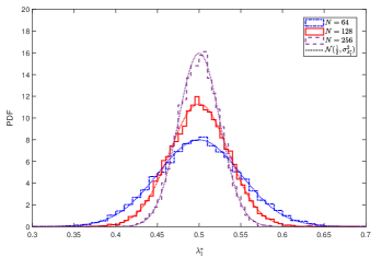
Figure 2: Histogram of the parameter $\lambda_{1}^{\star}$.

The previous observation will help us to derive an upper bound on the error rate performance of the -RQSSK system with optimized $\lambda_{1}^{\star}$. To see this, we present the BER performance of the -RQSSK system in Fig. 3. In this figure, for each value of $N$ we plot the simulation result for the system with optimized $\lambda_{1}^{\star}$ and also for a system which simply uses $\lambda_{1}=\frac{1}{2}$. As expected, the performance of the system with $\lambda_{1}=\frac{1}{2}$ provides an upper bound on the performance of the system with optimized $\lambda_{1}^{\star}$. This upper bound becomes very tight at low SNR, and also for larger values of $N$. In practice, the optimized $\lambda_{1}^{\star}$ is exactly equal to $\frac{1}{2}$ only when $m=n$, i.e., the same antenna is selected for both the real and imaginary parts.

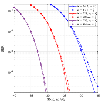
Figure 3: Impact of unoptimized $\lambda_{1}=\frac{1}{2}$ on the error rate performance of the -RQSSK system without polarity bits, for the case $N_{r}=4$.

IV Performance Analysis

IV-A RQSSK system without polarity bits

In this section, we analyze the theoretical ABEP of the -RQSSK system. For ease of exposition, we will initially assume that there are no polarity bits, i.e., $2\log_{2}N_{r}$ bits are transmitted per IM symbol, while the polarities are fixed and are not “detected” at the receiver. This analysis will focus on the GD receiver given by (4) and (5). Here we only perform the analysis for the detection of the antenna $m$ with active real part; due to the inherent symmetry in the expressions, it is easy to show that the ABEP expression for the detection of the antenna $n$ with active imaginary part is identical. Considering (4), the pairwise error probability (PEP) associated with the selected antenna $m$ and the detected antenna $\hat{m}\neq m$ is given by

$$\mbox{PEP}_{\mathrm{SSK}}\left(m,\hat{m}\right)=\Pr\left(\left(y_{m}^{\mathcal{R}}\right)^{2}<\left(y_{\hat{m}}^{\mathcal{R}}\right)^{2}\right)$$

$$=\Pr\left\{\left(\sqrt{E_{s}}\sum_{i=1}^{N}\left(h_{m,i}^{\mathcal{R}}\theta_{i}^{\mathcal{R}}-h_{m,i}^{\mathcal{I}}\theta_{i}^{\mathcal{I}}\right)+n_{m}^{\mathcal{R}}\right)^{2}<\right.$$

$$\quad\left.\left(\sqrt{E_{s}}\sum_{i=1}^{N}\left(h_{\hat{m},i}^{\mathcal{R}}\theta_{i}^{\mathcal{R}}-h_{\hat{m},i}^{\mathcal{I}}\theta_{i}^{\mathcal{I}}\right)+n_{\hat{m}}^{\mathcal{R}}\right)^{2}\right\}.$$ (30)

Considering $\left\{\theta_{i}^{\mathcal{R}}\right\}$ and $\left\{\theta_{i}^{\mathcal{I}}\right\}$ given in (28) and (29), and based on our discussion in the previous section regarding the average value of $\lambda_{1}^{\star}$, the PEP can be upper bounded as

$$\mbox{PEP}_{\mathrm{SSK}}\left(m,\hat{m}\right)\leq$$

$$\Pr\left(\left(\sqrt{E_{s}}Y+n_{m}^{\mathcal{R}}\right)^{2}<\left(\sqrt{E_{s}}\hat{Y}+n_{\hat{m}}^{\mathcal{R}}\right)^{2}\right),$$ (31)

where $Y=\sum_{i=1}^{N}Y_{i}=\sum_{i=1}^{N}\frac{A_{i}^{2}+C_{i}^{2}+A_{i}B_{i}+C_{i}D_{i}}{\sqrt{\left(A_{i}+B_{i}\right)^{2}+\left(C_{i}+D_{i}\right)^{2}}}$, $\hat{Y}=\sum_{i=1}^{N}\hat{Y}_{i}=\sum_{i=1}^{N}\left(\hat{A}_{i}\theta_{i}^{\mathcal{R}}+\hat{C}_{i}\theta_{i}^{\mathcal{I}}\right)$, and we define $\hat{A}_{i}=h_{\hat{m},i}^{\mathcal{R}}$ and $\hat{C}_{i}=-h_{\hat{m},i}^{\mathcal{I}}$ to simplify the notation. According to the CLT, $Y$ and $\hat{Y}$ both follow a normal distribution, i.e., $Y\sim\mathcal{N}\left(N\mathbb{E}\left\{Y_{i}\right\},N\mathbb{V}\left\{Y_{i}\right\}\right)$ and $\hat{Y}\sim\mathcal{N}\left(N\mathbb{E}\left\{\hat{Y}_{i}\right\},N\mathbb{V}\left\{\hat{Y}_{i}\right\}\right)$. Hence, the expected value and the variance of $Y_{i}$ and $\hat{Y}_{i}$ need to be evaluated. Since $B_{i}$ and $D_{i}$ depend on the selected antenna $n$ with active imaginary part, we need to consider three different cases: (i) $m\neq n$, $\hat{m}\neq n$, (ii) $m\neq n$, $\hat{m}=n$, and (iii) $m=n$, $\hat{m}\neq n$. For all three cases, the expected value and variance of $Y_{i}$ and $\hat{Y}_{i}$ can be derived analytically. Hence, by introducing RVs $Z_{1}=\sqrt{E_{s}}Y+n_{m}^{\mathcal{R}}$ and $Z_{2}=\sqrt{E_{s}}\hat{Y}+n_{\hat{m}}^{\mathcal{R}}$, the following theorems can be used to further analyze the PEP.

Theorem 1.

For case (i) where we have $m\neq n$ and $\hat{m}\neq n$, $Z_{1}$ and $Z_{2}$ follow a normal distribution as

$$Z_{1}\sim\mathcal{N}\left(\frac{N\sqrt{\pi E_{s}}}{2\sqrt{2}},\frac{\left(6-\pi\right)NE_{s}}{8}+\frac{N_{0}}{2}\right)$$

and

$$Z_{2}\sim\mathcal{N}\left(0,\frac{NE_{s}}{2}+\frac{N_{0}}{2}\right).$$

Proof:

The proof is provided in Appendix A. ∎

Theorem 2.

For case (ii) where we have $m\neq n$ and $\hat{m}=n$, $Z_{1}$ and $Z_{2}$ follow a normal distribution as

$$Z_{1}\sim\mathcal{N}\left(\frac{N\sqrt{\pi E_{s}}}{2\sqrt{2}},\frac{\left(6-\pi\right)NE_{s}}{8}+\frac{N_{0}}{2}\right)$$

and

$$Z_{2}\sim\mathcal{N}\left(0,\frac{NE_{s}}{4}+\frac{N_{0}}{2}\right).$$

Proof:

See Appendix B. ∎

Theorem 3.

For case (iii) where we have $m=n$ and $\hat{m}\neq n$, $Z_{1}$ and $Z_{2}$ follow a normal distribution as

$$Z_{1}\sim\mathcal{N}\left(\frac{N\sqrt{\pi E_{s}}}{2\sqrt{2}},\frac{\left(4-\pi\right)NE_{s}}{8}+\frac{N_{0}}{2}\right)$$

and

$$Z_{2}\sim\mathcal{N}\left(0,\frac{NE_{s}}{2}+\frac{N_{0}}{2}\right).$$

Proof:

See Appendix C. ∎

Therefore, the PEP can be expressed as

$$\mbox{PEP}_{\mathrm{SSK}}\left(m,\hat{m}\right)\leq \frac{N_{r}-2}{N_{r}}\Pr\left(Q<0|m\neq n,\hat{m}\neq n\right)$$

$$+\frac{1}{N_{r}}\Pr\left(Q<0|m\neq n,\hat{m}=n\right)$$

$$+\frac{1}{N_{r}}\Pr\left(Q<0|m=n,\hat{m}\neq n\right),$$ (32)

where $Q=Q_{1}-Q_{2}$ is the difference of the two non-central chi-square RVs $Q_{1}=Z_{1}^{2}$ and $Q_{2}=Z_{2}^{2}$ each having one degree of freedom. It can be easily proved that $Z_{1}$ and $Z_{2}$ are uncorrelated, i.e., $\mathbb{E}\left\{Z_{1}Z_{2}\right\}=\mathbb{E}\left\{Z_{1}\right\}\mathbb{E}\left\{Z_{2}\right\}=0$, and are therefore independent (recall that $Z_{1}$ and $Z_{2}$ are both normal RVs). The probability density function (PDF) and cumulative distribution function (CDF) of $Q$ can both be expressed in the form of an infinite series expansion; however, for odd values of the number of degrees of freedom the resulting expression is prohibitively complex [24]. Hence, we implement numerical methods and approximations to obtain the exact or approximated upper bounds on the PEP results. The Gil-Pelaez inversion formula [25, Eq. 4.4.1] is a numerical method that can be used to calculate the CDF of $Q$ as

$$F_{Q}\left(q\right)=\Pr\left(Q<q\right)=\frac{1}{2}-\frac{1}{\pi}\int_{0}^{\infty}t^{-1}\left(\phi_{Q}\left(t\right)e^{-jtq}\right)^{\mathcal{I}}\mathrm{d}t,$$ (33)

where $\phi_{Q}\left(t\right)$ is the characteristic function (CF) of $Q$ which can be derived from the Laplace transform (LT) of the PDF (see (47) in Appendix A, i.e., $\phi_{Q}\left(t\right)=\mathcal{L}_{-jt}\left(f_{Q}\left(q\right)\right)$. Hence, the exact upper bound expression on the PEP in (32) can be obtained by numerically evaluating the integral in (33) for $q=0$. However, to obtain further insight into the resulting PEP, we use Pearson’s approximation approach [26], where the distribution of a linear combination of non-central quadratic form of standard normal RVs $\left\{X_{i}\right\}$, i.e. $Q^{\prime}=\sum_{i=1}^{n}\delta_{i}\left(X_{i}+b_{i}\right)^{2}$, is approximated by that of a central chi-square RV, i.e.,

$$Q^{\prime}\approx\frac{c_{3}}{c_{2}}\chi_{v}^{2}-\frac{c_{2}^{2}}{c_{3}}+c_{1},$$ (34)

where $\approx$ here means “approximately distributed”,

$$c_{k}=\sum_{i=1}^{n}\delta_{i}^{k}\left(1+kb_{i}^{2}\right),\ k=1,2,3,$$ (35)

and

$$v=\frac{c_{2}^{3}}{c_{3}^{2}}.$$ (36)

We use this approach as it is simple yet remarkably accurate in both tails of the distribution. Hence, we obtain

$$\Pr\left(Q^{\prime}<q\right)\approxeq\Pr\left(\chi_{v}^{2}<\bar{q}\right),$$ (37)

where

$$\bar{q}=\left(q-c_{1}\right)\sqrt{\frac{v}{c_{2}}}+v.$$

Expressing $Q$ as the quadratic form $Q^{\prime}$, for case (i) where we have $m\neq n$ and $\hat{m}\neq n$, we obtain

$$\delta_{1}=\frac{\left(6-\pi\right)NE_{s}}{8}+\frac{N_{0}}{2},\ \delta_{2}=-\frac{NE_{s}}{2}-\frac{N_{0}}{2},$$

$$b_{1}^{2}=\frac{\pi N^{2}E_{s}}{\left(6-\pi\right)NE_{s}+4N_{0}},\ b_{2}=0.$$

These expressions can be similarly derived for cases (ii) and (iii). Substituting the corresponding variables for each case into (35) and (36), the details of the approximated chi-square RV can be derived accordingly. Hence, considering $q=0$ in (37), then for each case we have

$$\Pr\left(Q<0\right)\approxeq\Pr\left(\chi_{v}^{2}<\bar{q}\right)$$

$$=F\left(\bar{q};v\right)=\frac{\gamma\left(\frac{v}{2},\frac{\bar{q}}{2}\right)}{\Gamma\left(\frac{v}{2}\right)}=\frac{\gamma\left(\frac{v}{2},\frac{-c_{1}\sqrt{\nicefrac{{v}}{{c_{2}}}}+v}{2}\right)}{\Gamma\left(\frac{v}{2}\right)},$$ (38)

where $F\left(x;k\right)$ is the CDF of a chi-square RV with $k$ degrees of freedom, and $\gamma\left(s,x\right)=\int_{0}^{x}u^{s-1}e^{-s}du$ is the lower incomplete gamma function. Calculating (38) for all three cases in (32), we obtain an approximate upper bound on the PEP.

Considering the SNR range $N\frac{E_{s}}{N_{0}}\ll 1$ (which is of interest for large values of $N$; note that $N\gg 1$), then we have

$$v\approxeq\frac{2\left(\pi N^{2}\frac{E_{s}}{N_{0}}+4\right)^{3}}{9\left(\pi N^{2}\frac{E_{s}}{N_{0}}\right)^{2}},$$

$$\bar{q}\approxeq\frac{2\left(\pi N^{2}\frac{E_{s}}{N_{0}}+4\right)^{3}}{9\left(\pi N^{2}\frac{E_{s}}{N_{0}}\right)^{2}}-\frac{1}{6}\left(\pi N^{2}\frac{E_{s}}{N_{0}}+4\right).$$

Note that these approximate values of $v$ and $\bar{q}$ are equal in all three cases (i)-(iii). Then, for SNR values in the range $N^{2}\frac{E_{s}}{N_{0}}\gg 1$ (which is also valid in the range of interest for large values of $N$), we can write

$$v\approxeq\frac{2\pi N^{2}}{9}\frac{E_{s}}{N_{0}},\ \bar{q}\approxeq\frac{1}{4}v.$$

Then, it can be shown that the Chernoff bound on the lower tail of the CDF of a chi-square distribution $F\left(x;k\right)$, where $x=zk$, is given by

$$F\left(zk;k\right)\leq\left(ze^{1-z}\right)^{\frac{k}{2}},$$

hence, (38) can be expressed as

$$\mbox{PEP}_{\mathrm{SSK}}\left(m\rightarrow\hat{m}\right)\leq\Pr\left(Q<0\right)\lessapprox\left(\frac{2}{e^{\nicefrac{{3}}{{8}}}}\right)^{\frac{-2\pi N^{2}}{9}\frac{E_{s}}{N_{0}}},$$ (39)

which indicates the nature of the error rate performance enhancement that is obtained by increasing $N$. It is worth noting that (39) is similar in form to the Chernoff bound on the Q-function. Hence, we can conclude that the RIS-RQSSK system model behaves like a Gaussian channel with an average power gain that is proportional to $N^{2}$.

Finally, according to the union bound, the ABEP can be expressed as

$$\mbox{ABEP}\leq\frac{1}{N_{r}\log_{2}N_{r}}\sum_{m}\sum_{\hat{m}}\mbox{PEP}_{\mathrm{SSK}}\left(m\rightarrow\hat{m}\right)e\left(m\rightarrow\hat{m}\right),$$

where $e\left(m\rightarrow\hat{m}\right)$ is the Hamming distance between the binary representations of symbols $m$ and $\hat{m}$. It is worth pointing out that the PEP is independent of $m$ and $\hat{m}$; hence the ABEP can be re-expressed as

$$\mbox{ABEP}\leq\frac{N_{r}}{2}\mbox{PEP}_{\mathrm{SSK}}.$$ (40)

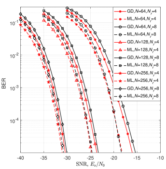
Figure 4: Comparison of the performance of the GD and ML detector in the proposed RIS-RQSSK system.

IV-B RQSSK including polarity bits

Next, we consider the case where two bits in each data packet of $2\left(\log_{2}N_{r}+1\right)$ bits is transmitted by the polarities of the real and imaginary “active” received signals. Similar to the case without polarity bits, we focus only on the real part (the analysis for the imaginary part is the same by symmetry). The pair $\left(m,d_{m}\right)$ represents the super-symbol comprised of SSK bits and the polarity bit, where $m$ denotes the antenna index with active real part and $d_{m}$ denotes the polarity bit. Hence, considering erroneous and correct detection of the antenna index separately, an upper bound on the ABEP can be derived as

$$\mbox{ABEP}\leq \frac{1}{2N_{r}\left(\log_{2}N_{r}+1\right)}$$

$$\sum_{(m,d)}\sum_{(\hat{m},\hat{d})}\mbox{PEP}\left(m,d\rightarrow\hat{m},\hat{d}_{m}\right)e\left(m,d\rightarrow\hat{m},\hat{d}_{m}\right)$$

$$= \frac{1}{\log_{2}N_{r}+1}\left[1-\left(N_{r}-1\right)\mbox{PEP}_{\mathrm{SSK}}\right]\mbox{PEP}_{\mathrm{POL}|m=\hat{m}}$$

$$+\frac{N_{r}\log_{2}N_{r}}{2\left(\log_{2}N_{r}+1\right)}\mbox{PEP}_{\mathrm{SSK}}\left(1-\mbox{PEP}_{\mathrm{POL}|m\neq\hat{m}}\right)$$

$$+\frac{\frac{N_{r}}{2}\log_{2}N_{r}+N_{r}-1}{\log_{2}N_{r}+1}\mbox{PEP}_{\mathrm{SSK}}\mbox{PEP}_{\mathrm{POL}|m\neq\hat{m}},$$ (41)

where $\mbox{PEP}_{\mathrm{POL}|m=\hat{m}}$ and $\mbox{PEP}_{\mathrm{POL}|m\neq\hat{m}}$ are the average PEP associated with the pair of polarity symbols $\left(d_{m},\hat{d}_{m}\right)$ conditioned on correct and erroneous detection of $m$, respectively, which are given by (42) and (43) shown on the next page.

$$\mbox{PEP}_{\mathrm{POL}|m=\hat{m}} =\frac{1}{N_{r}}\mathbb{E}_{Y}\left\{\mbox{Q}\left(\sqrt{Y^{2}\frac{2E_{s}}{N_{0}}}\right)|m=n\right\}+\frac{N_{r}-1}{N_{r}}\mathbb{E}_{Y}\left\{\mbox{Q}\left(\sqrt{Y^{2}\frac{2E_{s}}{N_{0}}}\right)|m\neq n\right\},$$ (42)

$$\mbox{PEP}_{\mathrm{POL}|m\neq\hat{m}} =\frac{1}{N_{r}-1}\mathbb{E}_{\hat{Y}}\left\{\mbox{Q}\left(\sqrt{\hat{Y}^{2}\frac{2E_{s}}{N_{0}}}\right)|\hat{m}=n\right\}+\frac{N_{r}-2}{N_{r}-1}\mathbb{E}_{\hat{Y}}\left\{\mbox{Q}\left(\sqrt{\hat{Y}^{2}\frac{2E_{s}}{N_{0}}}\right)|\hat{m}\neq n\right\}.$$ (43)

To calculate these average PEP, we use Craig’s alternative formula for the Q-function [27]. Hence, for an RV $V$ we can write

$$\mathbb{E}_{V}\left\{\mbox{Q}\left(\sqrt{V}\right)\right\}=\frac{1}{\pi}\int_{0}^{\nicefrac{{\pi}}{{2}}}\mathcal{M}_{V}\left(\frac{-1}{2\sin^{2}\phi}\right)\mathrm{d}\phi,$$ (44)

where $\mathcal{M}_{V}\left(s\right)$ is the moment generating function (MGF) of RV $V$. For each case in (42) and (43), the MGF of the received SNR can be calculated from the LT of the distribution function (see (47) in Appendix A). Finally, by computing the integral in (44) for all Q-functions in (42) and (43) and substituting (42) and (43), and exact (based on Gil-Pelaez formula) or approximate (based on Pearson approach or Chernoff bound) upper bound on $\mbox{PEP}_{\mathrm{SSK}}$ into (41), the desired ABEP for the -RQSSK system with polarity bits can be derived.

V Numerical Results

In this section, we demonstrate the performance of the proposed -RQSSK system through numerical results. As benchmarks, we consider the most prominent recently proposed RIS-based schemes which incorporate the concept of SM, namely RIS-RQRM [17] and RIS-SM [13] systems. First, in Fig. 4 we compare the performance of the RIS-RQSSK system where the GD and ML detector are implemented at the receiver. It can be seen that the GD performs fairly close to the ML detector in terms of the error rate. The performance gap between GD and ML detector reduces with an increasing number of RIS elements.

Then, Fig. 5 shows the BER performance of the proposed -RQSSK system as well as that of the benchmark schemes with $N_{r}=4$, for different values of the number of RIS elements $N$. The phase shifts for the proposed system are optimized according to the solution provided in Section III. Both the -RQSSK and RIS-RQRM systems exploit the polarity of the signals at the receiver to transmit two additional bits; however, in order to have a fair comparison, the RIS-SM system uses 16-QAM modulation in order to compensate for the additional bits transmitted by the quadrature branch. Hence, the data rate is $R=6$  bits per channel use (bpcu) in all of the considered schemes. We perform GD at the receiver in all scenarios to detect the spatial symbols, and hence CSI is not required in the -RQSSK and RIS-RQRM systems, while RIS-SM needs to know the channel amplitudes in order to detect the QAM symbols, i.e., partial channel knowledge is required.

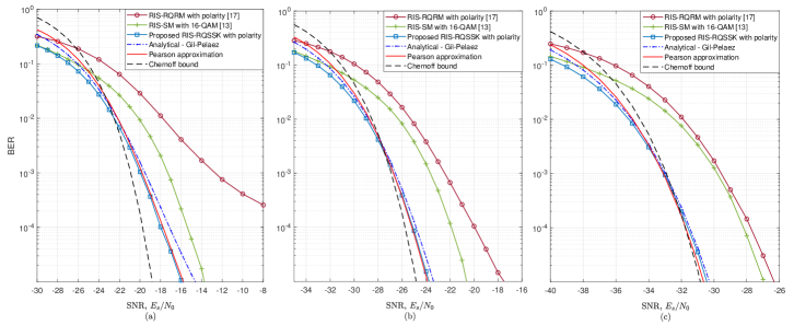
Figure 5: Analytical and simulation results of the proposed -RQSSK system, and comparison of the performance with that of RIS-RQRM and RIS-SM systems. Here $N_{r}=4$ and $R=6$. (a) $N=64$, (b) $N=128$, (c) $N=256$.

It can be observed that the proposed system significantly outperforms the RIS-RQRM system which is an alternative quadrature-based approach for spatial modulation. However, in RIS-RQRM, the RIS elements are divided into two equal groups each of which targets either the real or the imaginary part of the selected receive antenna, which clearly deteriorates the performance of the system. The gain of the proposed scheme over RIS-RQRM is 6.2 dB and 4.1 dB for systems with $N=128$ and $N=256$, respectively, at a BER of $10^{-5}$. In the system with $N=64$, a larger gain is obtained, since in the RIS-RQRM system, the number of RIS elements assisting each activated real/imaginary part is $N=32$, which results in an error floor in the moderate BER range. The proposed -RQSSK also provides superior performance to RIS-SM. This superiority is due to the fact that the RIS-SM system uses 16-QAM modulation to achieve $R=6$ bpcu, which results in a diminishing BER performance due to the smaller minimum Euclidean distance between different constellation points. The proposed -RQSSK system achieves 2.4 dB, 3.2 dB and 3.5 dB performance improvement over the RIS-SM system for systems with $N=64$, $N=128$ and $N=256$, respectively. In this figure, we also plot the analytical and approximate results discussed in the previous section. The exact results based on the Gil-Pelaez inversion formula validate the simulation curves for the proposed system. The tiny difference between the simulation and Gil-Pelaez curves is caused by the fact that we use $\lambda_{1}=\frac{1}{2}$ in the theoretical analysis, while the optimized $\lambda_{1}^{\star}$ is used in the simulations. This difference becomes smaller with increasing $N$, as expected (c.f., Fig. 3). In addition, it can be seen that the results based on the Pearson approximation approach are very close to that of the Gil-Pelaez formula, especially for larger values of $N$. However, as expected, the resulting Chernoff bounds are not quite valid at small values of $N$, as in this case the conditions on the SNR range are not satisfied. However, for large values of $N$, i.e., $N\geq 256$, the gap between the Chernoff bound and the theoretical curve becomes small enough that it can be neglected.

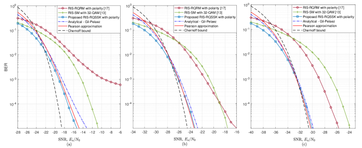
Figure 6: Analytical and simulation results of the proposed -RQSSK system, and comparison of the performance with that of RIS-RQRM and RIS-SM systems. Here $N_{r}=8$ and $R=8$. (a) $N=64$, (b) $N=128$, (c) $N=256$.

In Fig. 6, we plot the corresponding results for a system with $N_{r}=8$. Here the RIS-SM system uses 32-QAM, and hence the data rate is $R=8$ bpcu in all scenarios. The results show that the BER of the proposed -RQSSK system significantly outperforms that of the other schemes. Also, we see that this improvement increases with increasing $N_{r}$. This is due to the fact that the number of RIS elements in the RIS-RQRM system becomes smaller compared to the number of receive antennas, and therefore the RIS system cannot efficiently perform beamforming toward the target receive antenna. Besides, the use of 32-QAM in the RIS-SM system results in a very small minimum Euclidean distance which degrades the performance of the system, such that it performs even worse than RIS-RQRM in the case where $N=256$. The proposed -RQSSK designs provide 7.2 dB and 4.4 dB improvement over RIS-RQRM with $N=128$ and $N=256$, respectively, and 4.5 dB, 5.6 dB and 6.2 dB gain over RIS-SM with $N=64$, $N=128$ and $N=256$, respectively. It is worth noting that the RIS-SM scheme requires partial CSI at the receiver, while the GD in the proposed -RQSSK system performs CSI-free detection. Finally, it can be seen that compared to the system with $N_{r}=4$, the gap between the theoretical and numerical curves is slightly increased. The reason for this is that in a system with $N_{r}=4$, the coincidence of $m=n$ is more likely to occur, which, as previously mentioned, yields $\lambda_{1}^{\star}=\frac{1}{2}$, the same value that is used in the theoretical analysis.

VI Conclusion

In this paper, we introduced a novel IM scheme for RIS-assisted wireless communications, called -RQSSK, in which SSK was performed independently in both the real and imaginary dimensions. The key advantage of this approach is that all RIS elements perform beamforming onto the real and imaginary part of the received signal at the selected antennas, respectively. Therefore, in addition to realizing an enhancement in the spectral efficiency, the error rate performance is also improved. We also defined and formulated a max-min optimization problem to maximize the instantaneous SNR components at the selected antennas. We provided an analytical solution for this non-convex problem, such that the multi-variable optimization problem can be transformed to a simple single-variable equation. We analyzed the ABEP of the proposed scheme, and derived analytical upper bounds on the approximate ABEP. The BER performance of the proposed -RQSSK system has been demonstrated through extensive numerical simulations. Our numerical results have shown that the proposed -RQSSK system enormously outperforms the recent prominent benchmark schemes such as RIS-SM and RIS-RQRM, thus providing an approach for RIS-aided wireless communications which exhibits a high energy efficiency without compromising on spectral efficiency. This low-powered single-antenna AP system can be a potential candidate for small cells in cellular networks. Moreover, in addition to the use of a simple GD at the receiver, reliable communications can be achieved with simpler channel codes which require lower complexity at the receiver. As a result, the proposed approach can be adopted to serve user devices in the downlink that are energy-constrained and require low-complexity receiver algorithms. Finally, an interesting direction of future research is to develop the proposed system in order to support IQ modulation as well as index modulation to obtain higher data rates.

Appendix A Proof of Theorem 1

Here we analyze the expected value and variance of $Y_{i}$ and $\hat{Y}_{i}$ where $m\neq n$ and $\hat{m}\neq n$ (case (i)), which are further used to evaluate the expected value and variance of $Z_{1}$ and $Z_{2}$.

A-A Expected value of $Y_{i}=\frac{A_{i}^{2}+C_{i}^{2}+A_{i}B_{i}+C_{i}D_{i}}{\sqrt{\left(A_{i}+B_{i}\right)^{2}+\left(C_{i}+D_{i}\right)^{2}}}$

$Y_{i}$ consists of four terms defined as

$$W_{1}\triangleq\frac{A^{2}}{\sqrt{Z}},\;W_{2}\triangleq\frac{C^{2}}{\sqrt{Z}},\;W_{3}\triangleq\frac{AB}{\sqrt{Z}},\;W_{4}\triangleq\frac{CD}{\sqrt{Z}},$$

where we define $Z\triangleq(A+B)^{2}+(C+D)^{2}$ and also we omit the index $i$ in order to simplify the notation. In the following, we evaluate the expected value of each term individually.

According to the law of total expectation, the expected value of $W_{1}$ can be given by

$$\mathbb{E}\left\{W_{1}\right\}=\mathbb{E}_{A}\left\{\mathbb{E}_{W_{1}|A}\left\{W_{1}|A\right\}\right\}$$

$$=\mathbb{E}_{A}\left\{\mathbb{E}_{W_{1}|A}\left\{\frac{A^{2}}{\sqrt{Z}}|A\right\}\right\}=\mathbb{E}_{A}\left\{A^{2}\mathbb{E}_{Z|A}\left\{Z^{-\frac{1}{2}}|A\right\}\right\},$$ (45)

where $\mathbb{E}_{Z|A}\left\{Z^{-\frac{1}{2}}|A\right\}$ is the inverse-fractional moment of $Z$ where $A$ is given, i.e., where $A$ is a constant. For a given $A$, the RV $(A+B)$ is normal with mean $A$ and variance $\frac{1}{2}$, i.e., $\left(A+B\right)\sim\mathcal{N}\left(A,\frac{1}{2}\right)$, and also $\left(C+D\right)$ is distributed according to $\mathcal{N}\left(0,1\right)$. Hence, the RV $(Z|A)$ is the sum of two independent chi-square RVs each having one degree of freedom, i.e.,

$$\left(Z|A\right)\sim\chi_{1}^{2}\left(A^{2}\right)+\chi_{1}^{2}.$$

To compute the inverse and fractional moment of $\left(Z|A\right)$, we use the definition of the gamma function to write [25]

$$\mathbb{E}_{Z|A}\left\{Z^{-c}|A\right\} =\mathbb{E}_{Z|A}\left\{\frac{1}{\Gamma\left(c\right)}\int_{0}^{\infty}s^{c-1}e^{-sZ}\mathrm{d}s|A\right\}$$

$$=\frac{1}{\Gamma\left(c\right)}\int_{0}^{\infty}s^{c-1}\mathbb{E}_{Z|A}\left\{e^{-sZ}|A\right\}\mathrm{d}s.$$ (46)

However, $\mathbb{E}_{Z|A}\left\{e^{-sZ}|A\right\}$ is the MGF of $\left(Z|A\right)$, $\mathcal{M}_{Z|A}\left(-s\right)$, or the LT of $f_{Z}\left(Z|A\right)$, $\mathcal{L}_{s}\left(f_{Z}\left(Z|A\right)\right)$. We know that the LT of the PDF of the sum of independent RVs is the multiplication of the LT of their individual PDFs, and that the LT of the PDF of an RV $X=\sum_{i=1}^{n}X_{i}^{2}$ with $X_{i}\sim\mathcal{N}\left(\mu_{i},\sigma^{2}\right)$ is given by

$$\mathcal{L}_{s}\left(f_{X}(X)\right)=\left(\frac{1}{1+2\sigma^{2}s}\right)^{\frac{n}{2}}\exp\left(\frac{-\mu^{2}s}{1+2\sigma^{2}s}\right),$$ (47)

where $\mu^{2}=\sum_{i=1}^{n}\mu_{i}^{2}$. Hence, the LT of $f_{Z}\left(Z|A\right)$ can be expressed as

$$\mathcal{L}_{s}\left(f_{Z}\left(Z|A\right)\right)=\left(\frac{1}{1+2s}\right)^{\frac{1}{2}}\left(\frac{1}{1+s}\right)^{\frac{1}{2}}\exp\left(\frac{-A^{2}s}{1+s}\right).$$ (48)

Then, (45) can be written as (49) shown on the next page.

$$\mathbb{E}\left\{W_{1}\right\} =\mathbb{E}_{A}\left\{\frac{A^{2}}{\Gamma\left(\frac{1}{2}\right)}\int_{0}^{\infty}s^{\frac{1}{2}-1}\left(\frac{1}{1+2s}\right)^{\frac{1}{2}}\left(\frac{1}{1+s}\right)^{\frac{1}{2}}\exp\left(\frac{-A^{2}s}{1+s}\right)\mathrm{d}s\right\}$$

$$=\frac{1}{\Gamma\left(\frac{1}{2}\right)}\int_{-\infty}^{\infty}A^{2}\left(\int_{0}^{\infty}s^{\frac{1}{2}-1}\left(\frac{1}{1+2s}\right)^{\frac{1}{2}}\left(\frac{1}{1+s}\right)^{\frac{1}{2}}\exp\left(\frac{-A^{2}s}{1+s}\right)\mathrm{d}s\right)f_{A}\left(A\right)\mathrm{d}A.$$ (49)

Considering $f_{A}\left(A\right)=\frac{1}{\Gamma\left(\frac{1}{2}\right)}\exp\left(-A^{2}\right)$, and changing the order of integrals we have

$$\mathbb{E}\left\{W_{1}\right\}= \frac{1}{\Gamma^{2}\left(\frac{1}{2}\right)}\int_{0}^{\infty}s^{\frac{1}{2}-1}\left(\frac{1}{1+2s}\right)^{\frac{1}{2}}\left(\frac{1}{1+s}\right)^{\frac{1}{2}}$$

$$\left(\int_{-\infty}^{\infty}A^{2}\exp\left(-A^{2}\frac{1+2s}{1+s}\right)\mathrm{d}A\right)\mathrm{d}s.$$

Since $\int_{-\infty}^{\infty}x^{2}\exp\left(-\frac{x^{2}}{2\sigma^{2}}\right)\mathrm{d}x=\Gamma\left(\frac{1}{2}\right)\sigma^{2}\sqrt{2\sigma^{2}}$, we have $\int_{-\infty}^{\infty}A^{2}\exp\left(-A^{2}\frac{1+2s}{1+s}\right)\mathrm{d}A=\frac{\Gamma\left(\frac{1}{2}\right)}{2}\left(\frac{1+s}{1+2s}\right)^{\frac{3}{2}}$; hence

$$\mathbb{E}\left\{W_{1}\right\}= \frac{1}{2\Gamma\left(\frac{1}{2}\right)}\int_{0}^{\infty}s^{\frac{1}{2}-1}\frac{1+s}{\left(1+2s\right)^{2}}\mathrm{d}s$$

$$= \frac{1}{2\Gamma\left(\frac{1}{2}\right)}\left(\frac{1}{2}\int_{0}^{\infty}s^{\frac{1}{2}-1}\left(1+2s\right)^{-1}\mathrm{d}s\right.$$

$$\left.+\frac{1}{2}\int_{0}^{\infty}s^{\frac{1}{2}-1}\left(1+2s\right)^{-2}\mathrm{d}s\right).$$

Considering the type-2 beta function defined as $B\left(\alpha,\beta\right)=\int_{0}^{\infty}\frac{t^{\alpha-1}}{\left(1+t\right)^{\alpha+\beta}}\mathrm{d}t=\frac{\Gamma\left(\alpha\right)\Gamma\left(\beta\right)}{\Gamma\left(\alpha+\beta\right)}$, with some minor manipulation we obtain

$$\mathbb{E}\left\{W_{1}\right\} =\frac{1}{2\Gamma\left(\frac{1}{2}\right)}\left(\frac{1}{2\sqrt{2}}\frac{\Gamma\left(\frac{1}{2}\right)\Gamma\left(\frac{1}{2}\right)}{\Gamma\left(1\right)}+\frac{1}{2\sqrt{2}}\frac{\Gamma\left(\frac{1}{2}\right)\Gamma\left(\frac{3}{2}\right)}{\Gamma\left(2\right)}\right)$$

$$=\frac{3\sqrt{\pi}}{8\sqrt{2}}.$$

By symmetry it is clear that $\mathbb{E}\left\{W_{2}\right\}=\mathbb{E}\left\{W_{1}\right\}$.

Next we determine $\mathbb{E}\left\{W_{3}=\frac{AB}{\sqrt{Z}}\right\}$. Considering the law of total expectation and expanding this for multiple RVs, we have

$$\mathbb{E}\left\{W_{3}\right\} =\mathbb{E}_{(A,B)}\left\{\mathbb{E}_{W_{3}|(A,B)}\left\{W_{3}|(A,B)\right\}\right\}$$

$$=\mathbb{E}_{A}\left\{A\mathbb{E}_{B}\left\{B\mathbb{E}_{Z|(A,B)}\left\{Z^{-\frac{1}{2}}|(A,B)\right\}\right\}\right\}.$$

Now, given $(A,B)$, $Z$ is the sum of the central chi-square RV $\left(C+D\right)^{2}$ and the constant $\left(A+B\right)^{2}$. Hence, $Z=\bar{Z}+\left(A+B\right)^{2}$, where $\bar{Z}=(C+D)^{2}$, then we have $f_{Z}\left(Z|(A,B)\right)=f_{\bar{Z}}\left(Z-\left(A+B\right)^{2}\right)$. Therefore,

$$\mathcal{L}_{s}\left(f_{Z}\left(Z|(A,B)\right)\right) =\mathcal{L}_{s}\left(f_{\bar{Z}}\left(Z-\left(A+B\right)^{2}\right)\right)$$

$$=\exp\left(-\left(A+B\right)^{2}s\right)\mathcal{L}_{s}\left(f_{\bar{Z}}\left(\bar{Z}\right)\right).$$

Hence, given (47), the LT of $f_{Z}\left(Z|(A,B)\right)$ can be expressed as

$$\mathcal{L}_{s}\left(f_{Z}\left(Z|(A,B)\right)\right) =\exp\left(-\left(A+B\right)^{2}s\right)\mathcal{L}_{s}\left(f_{\bar{Z}}\left(\bar{Z}\right)\right)$$

$$=\left(\frac{1}{1+2s}\right)^{\frac{1}{2}}\exp\left(-\left(A+B\right)^{2}s\right).$$ (50)

Using (46), we have

$$\mathbb{E}\left\{W_{3}\right\}= \mathbb{E}_{A}\left\{A\mathbb{E}_{B}\left\{\frac{B}{\Gamma\left(\frac{1}{2}\right)}\int_{0}^{\infty}s^{\frac{1}{2}-1}\left(\frac{1}{1+2s}\right)^{\frac{1}{2}}\right.\right.$$

$$\exp\left(-\left(A+B\right)^{2}s\right)\mathrm{d}s\Biggr{\}}\Biggr{\}}.$$

Using $f_{A}\left(A\right)=\frac{1}{\Gamma\left(\frac{1}{2}\right)}\exp\left(-A^{2}\right)$ and $f_{B}\left(B\right)=\frac{1}{\Gamma\left(\frac{1}{2}\right)}\exp\left(-B^{2}\right)$, and after some manipulation we can write

$$\mathbb{E}\left\{W_{3}\right\}= \frac{1}{\Gamma^{3}\left(\frac{1}{2}\right)}\int_{0}^{\infty}s^{\frac{1}{2}-1}\left(\frac{1}{1+2s}\right)^{\frac{1}{2}}\Biggl{[}\int_{-\infty}^{\infty}A\exp\Biggl{(}-A^{2}\frac{1+2s}{1+s}\Biggr{)}$$

$$\Biggl{(}\int_{-\infty}^{\infty}B\exp\Biggl{(}-\frac{\left(B+\frac{As}{1+s}\right)^{2}}{\frac{1}{1+s}}\Biggr{)}\mathrm{d}B\Biggr{)}\mathrm{d}A\Biggr{]}\mathrm{d}s.$$ (51)

Since $\int_{-\infty}^{\infty}x\exp\left(-\frac{\left(x-\mu\right)^{2}}{2\sigma^{2}}\right)\mathrm{d}x=\Gamma\left(\frac{1}{2}\right)\mu\sqrt{2\sigma^{2}}$, the inner integral over $B$ can be evaluated as

$$\int_{-\infty}^{\infty}B\exp\left(-\frac{\left(B+\frac{As}{1+s}\right)^{2}}{\frac{1}{1+s}}\right)\mathrm{d}B=-\Gamma\left(\frac{1}{2}\right)\frac{As}{1+s}\left(\frac{1}{1+s}\right)^{\frac{1}{2}}.$$

Substituting this into (51), the expected value of $W_{3}$ is given by

$$\mathbb{E}\left\{W_{3}\right\}= \frac{-1}{\Gamma^{2}\left(\frac{1}{2}\right)}\int_{0}^{\infty}s^{\frac{3}{2}-1}\left(\frac{1}{1+2s}\right)^{\frac{1}{2}}\left(\frac{1}{1+s}\right)^{\frac{3}{2}}$$

$$\left(\int_{-\infty}^{\infty}A^{2}\exp\left(-A^{2}\frac{1+2s}{1+s}\right)\mathrm{d}A\right)\mathrm{d}s$$

$$= \frac{-1}{2\Gamma\left(\frac{1}{2}\right)}\int_{0}^{\infty}s^{\frac{3}{2}-1}\left(\frac{1}{1+2s}\right)^{2}\mathrm{d}s$$

$$= \frac{-1}{4\sqrt{2}\Gamma\left(\frac{1}{2}\right)}B\left(\frac{3}{2},\frac{1}{2}\right)=-\frac{\sqrt{\pi}}{8\sqrt{2}}.$$

Also, by symmetry we have $\mathbb{E}\{W_{4}\}=\mathbb{E}\{W_{3}\}$. Therefore, the expected value of $Y_{i}$ is given by

$$\mathbb{E}\left\{Y_{i}\right\}=2\left(\mathbb{E}\left\{W_{1}\right\}+\mathbb{E}\left\{W_{3}\right\}\right)=\frac{\sqrt{\pi}}{2\sqrt{2}}.$$ (52)

A-B Variance of $Y_{i}=\frac{A_{i}^{2}+C_{i}^{2}+A_{i}B_{i}+C_{i}D_{i}}{\sqrt{\left(A_{i}+B_{i}\right)^{2}+\left(C_{i}+D_{i}\right)^{2}}}$

The variance of $Y_{i}$ is given by

$$\mathbb{V}\left\{Y_{i}\right\}=\mathbb{E}\left\{Y_{i}^{2}\right\}-\mathbb{E}\left\{Y_{i}\right\}^{2}.$$

However, $\mathbb{E}\left\{Y_{i}\right\}$ is given in (52); hence, only the expected value of $Y_{i}^{2}$ needs to be evaluated. We separate the expression of $Y_{i}^{2}$ into 4 terms as

$$U_{1}\triangleq\frac{A^{4}+A^{2}B^{2}+2A^{3}B}{Z},\;U_{2}\triangleq\frac{C^{4}+C^{2}D^{2}+2C^{3}D}{Z},$$

$$U_{3}\triangleq\frac{2A^{2}CD+2A^{2}C^{2}}{Z},\;U_{4}\triangleq\frac{2ABC^{2}+2ABCD}{Z}.$$

We can analyze the expected values of $U_{1}$ to $U_{4}$ separately. However, it is trivial that $\mathbb{E}\left\{U_{1}\right\}=\mathbb{E}\left\{U_{2}\right\}$. Therefore, in the following we calculate the expected values of $U_{1}$, $U_{3}$ and $U_{4}$.

• Expected value of $U_{1}=\frac{A^{4}+A^{2}B^{2}+2A^{3}B}{Z}$

According to the law of total expectation, we have

$$\mathbb{E}\left\{U_{1}\right\}=$$

$$\mathbb{E}_{(A,B)}\left\{\left(A^{4}+A^{2}B^{2}+2A^{3}B\right)\mathbb{E}_{Z|(A,B)}\left\{Z^{-1}|(A,B)\right\}\right\}.$$

From (46) and (50), $\mathbb{E}\left\{U_{1}\right\}$ can be expressed as

$$\mathbb{E}\left\{U_{1}\right\}=$$

$$\frac{1}{\Gamma^{2}\left(\frac{1}{2}\right)}\int_{0}^{\infty}\left(\frac{1}{1+2s}\right)^{\frac{1}{2}}\Biggl{[}\int_{-\infty}^{\infty}\int_{-\infty}^{\infty}\left(A^{4}+A^{2}B^{2}+2A^{3}B\right)$$

$$\exp\Biggl{(}-\frac{\left(B+\frac{As}{1+s}\right)^{2}}{\frac{1}{1+s}}\Biggr{)}\exp\biggl{(}-A^{2}\frac{1+2s}{1+s}\biggr{)}\mathrm{d}B\mathrm{d}A\Biggr{]}\mathrm{d}s$$

$$=\frac{\Gamma\left(\frac{5}{2}\right)}{\Gamma\left(\frac{1}{2}\right)}\int_{0}^{\infty}\frac{1}{\left(1+2s\right)^{3}}\mathrm{d}s+\frac{1}{4}\int_{0}^{\infty}\frac{1}{\left(1+2s\right)^{2}}\mathrm{d}s$$

$$=\frac{3}{4}\cdot\frac{1}{4}+\frac{1}{4}\cdot\frac{1}{2}=\frac{5}{16}.$$

• Expected value of $U_{3}=\frac{2A^{2}CD+2A^{2}C^{2}}{Z}$

$\mathbb{E}\left\{U_{3}\right\}$ can be evaluated as (53) shown on the next page.

$$\mathbb{E}\left\{U_{3}\right\}= \mathbb{E}_{(A,C,D)}\left\{\left(2A^{2}CD+2A^{2}C^{2}\right)\mathbb{E}_{Z|(A,C,D)}\left\{Z^{-1}|(A,C,D)\right\}\right\}$$

$$= \frac{2}{\Gamma^{3}\left(\frac{1}{2}\right)}\int_{-\infty}^{\infty}\int_{-\infty}^{\infty}\int_{-\infty}^{\infty}\left(A^{2}CD+A^{2}C^{2}\right)\left(\int_{0}^{\infty}\mathcal{L}_{s}\left(f_{Z|(A,C,D)}\right)\mathrm{d}s\right)\exp\left(-D^{2}\right)\exp\left(-C^{2}\right)\exp\left(-A^{2}\right)\mathrm{d}D\mathrm{d}C\mathrm{d}A$$

$$= \frac{2}{\Gamma^{3}\left(\frac{1}{2}\right)}\int_{0}^{\infty}\left(\frac{1}{1+s}\right)^{\frac{1}{2}}\left(\int_{-\infty}^{\infty}A^{2}\exp\left(-A^{2}\frac{1+2s}{1+s}\right)\mathrm{d}A\right)$$

$$\left(\int_{-\infty}^{\infty}\int_{-\infty}^{\infty}\left(CD+C^{2}\right)\exp\left(-\frac{\left(D+\frac{Cs}{1+s}\right)^{2}}{\frac{1}{1+s}}\right)\exp\left(-C^{2}\frac{1+2s}{1+s}\right)\mathrm{d}D\mathrm{d}C\right)\mathrm{d}s$$

$$= \frac{1}{2}\int_{0}^{\infty}\frac{1+s}{\left(1+2s\right)^{3}}\mathrm{d}s=\frac{3}{16}.$$ (53)

• Expected value of $U_{4}=\frac{2ABC^{2}+2ABCD}{Z}$

We can write

$$\mathbb{E}\left\{U_{4}\right\}=$$

$$\mathbb{E}_{(A,B,C)}\left\{2ABC\mathbb{E}_{(U_{4}/2ABC)|(A,B,C)}\left\{\frac{C+D}{Z}|(A,B,C)\right\}\right\}.$$

In contrast to the previous calculations where an inverse-fractional moment of a quadratic function of an RV or RVs were required, here the first moment of a quotient of two functions of an RV needs to be evaluated. Positive integer moments of $R=\frac{Q_{1}}{Q_{2}}$ can be calculated by [25, Eq. 4.5a.2]

$$\mathbb{E}\left\{R^{c}\right\}=\frac{1}{\Gamma\left(c\right)}\int_{0}^{\infty}s_{2}^{c-1}\left.\left[\frac{\partial^{c}}{\partial s_{1}^{c}}\mathcal{M}_{Q_{1},Q_{2}}\left(s_{1},-s_{2}\right)\right]\right|_{s_{1}=0}\mathrm{d}s_{2},$$ (54)

where $\mathcal{M}_{Q_{1},Q_{2}}\left(s_{1},s_{2}\right)$ is the joint MGF of $Q_{1}$ and $Q_{2}$. Further, the joint MGF of quadratic forms $Q_{1}=\mathbf{x}^{T}\mathbf{A}_{1}\mathbf{x}+\mathbf{a}_{1}^{T}\mathbf{x}+d_{1}$ and $Q_{2}=\mathbf{x}^{T}\mathbf{A}_{2}\mathbf{x}+\mathbf{a}_{2}^{T}\mathbf{x}+d_{2}$, where $\mathbf{x}\sim\mathcal{N}_{p}\left(\boldsymbol{\mu},\boldsymbol{\Sigma}\right)$ is a length-$p$ normal random vector, is given by (55) shown on the next page [25, Eq. 3.2c.5].

$$\mathcal{M}_{Q_{1},Q_{2}}\left(s_{1},s_{2}\right)= \det\left(\mathbf{I}-2s_{1}\mathbf{A}_{1}\boldsymbol{\Sigma}-2s_{2}\mathbf{A}_{2}\boldsymbol{\Sigma}\right)^{-\frac{1}{2}}\exp\left[-\frac{1}{2}\left(\boldsymbol{\mu}^{T}\boldsymbol{\Sigma}^{-1}\boldsymbol{\mu}-2s_{1}d_{1}-2s_{2}d_{2}\right)+\right.$$

$$\left.\frac{1}{2}\left(s_{1}\boldsymbol{\Sigma}\mathbf{a}_{1}+s_{2}\boldsymbol{\Sigma}\mathbf{a}_{2}+\boldsymbol{\mu}\right)^{T}\left(\mathbf{I}-2s_{1}\mathbf{A}_{1}\boldsymbol{\Sigma}-2s_{2}\mathbf{A}_{2}\boldsymbol{\Sigma}\right)^{-1}\boldsymbol{\Sigma}^{-1}\left(s_{1}\boldsymbol{\Sigma}\mathbf{a}_{1}+s_{2}\boldsymbol{\Sigma}\mathbf{a}_{2}+\boldsymbol{\mu}\right)\right].$$ (55)

Hence, the joint MGF of $Q_{1}=C+D$ and $Q_{2}=\left(A+B\right)^{2}+\left(C+D\right)^{2}$, where $(A,B,C)$ is given, can be expressed as

$$\mathcal{M}_{(Q_{1},Q_{2})|(A,B,C)}\left(s_{1},s_{2}\right)=$$

$$\frac{1}{\left(1-s_{2}\right)^{\frac{1}{2}}}\exp\left(-C^{2}+s_{2}\left(A+B\right)^{2}+\frac{\left(\frac{1}{2}s_{1}+C\right)^{2}}{\left(1-s_{2}\right)}\right).$$

Substituting this into (54) and considering $c=1$, we can write

$$\mathbb{E}_{(U_{4}/2ABC)|(A,B,C)}\left\{\frac{C+D}{Z}|(A,B,C)\right\}=$$

$$\int_{0}^{\infty}\frac{C}{\left(1+s_{2}\right)^{\frac{3}{2}}}\exp\left(-C^{2}\frac{s_{2}}{1+s_{2}}\right)\exp\left(-\left(A+B\right)^{2}s_{2}\right)\mathrm{d}s_{2}.$$

Then, $\mathbb{E}\left\{U_{4}\right\}$ can be evaluated as (56) shown on the next page.

$$\mathbb{E}\left\{U_{4}\right\}= \frac{2}{\Gamma^{3}\left(\frac{1}{2}\right)}\int_{-\infty}^{\infty}\int_{-\infty}^{\infty}\int_{-\infty}^{\infty}ABC\Biggl{[}\int_{0}^{\infty}\frac{C}{\left(1+s_{2}\right)^{\frac{3}{2}}}\exp\biggl{(}-C^{2}\frac{s_{2}}{1+s_{2}}\biggr{)}\exp\left(-\left(A+B\right)^{2}s_{2}\right)\mathrm{d}s_{2}\Biggr{]}$$

$$\exp\left(-C^{2}\right)\exp\left(-B^{2}\right)\exp\left(-A^{2}\right)\mathrm{d}C\mathrm{d}B\mathrm{d}A$$

$$= \frac{2}{\Gamma^{3}\left(\frac{1}{2}\right)}\int_{0}^{\infty}\frac{1}{\left(1+s_{2}\right)^{\frac{3}{2}}}\Biggl{[}\int_{-\infty}^{\infty}\int_{-\infty}^{\infty}AB\exp\Biggl{(}-\frac{\Bigl{(}B+\frac{As_{2}}{1+s_{2}}\Bigr{)}^{2}}{\frac{1}{1+s_{2}}}\Biggr{)}\exp\left(-A^{2}\frac{1+2s_{2}}{1+s_{2}}\right)\mathrm{d}B\mathrm{d}A\Biggr{]}$$

$$\biggl{(}\int_{-\infty}^{\infty}C^{2}\exp\Bigl{(}-C^{2}\frac{1+2s_{2}}{1+s_{2}}\Bigr{)}\mathrm{d}C\biggr{)}\mathrm{d}s_{2}$$

$$= -\frac{1}{2}\int_{0}^{\infty}\frac{s_{2}}{\left(1+2s_{2}\right)^{3}}\mathrm{d}s_{2}=-\frac{1}{16}.$$ (56)

Therefore, the variance of $Y_{i}$ is calculated as

$$\mathbb{V}\left\{Y_{i}\right\} =\mathbb{E}\left\{Y_{i}^{2}\right\}-\mathbb{E}\left\{Y_{i}\right\}^{2}$$

$$=\left(2\cdot\frac{5}{16}+\frac{3}{16}-\frac{1}{16}\right)-\left(\frac{\sqrt{\pi}}{2\sqrt{2}}\right)^{2}=\frac{6-\pi}{8}.$$

A-C Expected value of $\hat{Y}_{i}=\hat{A}_{i}\theta_{i}^{\mathcal{R}}+\hat{C}_{i}\theta_{i}^{\mathcal{I}}$

Since $\theta_{i}^{\mathcal{R}}$ and $\theta_{i}^{\mathcal{I}}$ are independent of $\hat{A}_{i}$ and $\hat{C_{i}}$, then $\mathbb{E}\left\{\hat{Y}_{i}\right\}$ is calculated as

$$\mathbb{E}\left\{\hat{Y}_{i}\right\}=\mathbb{E}\left\{\hat{A}_{i}\right\}\mathbb{E}\left\{\theta_{i}^{\mathcal{R}}\right\}+\mathbb{E}\left\{\hat{C}_{i}\right\}\mathbb{E}\left\{\theta_{i}^{\mathcal{I}}\right\}=0.$$

A-D Variance of $\hat{Y}_{i}=\hat{A}_{i}\theta_{i}^{\mathcal{R}}+\hat{C}_{i}\theta_{i}^{\mathcal{I}}$

The variance of $\hat{Y}_{i}$ is given by

$$\mathbb{V}\left\{\hat{Y}_{i}\right\}= \mathbb{E}\left\{\hat{Y}_{i}^{2}\right\}$$

$$= \mathbb{E}\left\{\hat{A}_{i}^{2}\right\}\mathbb{E}\left\{\left(\theta_{i}^{\mathcal{R}}\right)^{2}\right\}+\mathbb{E}\left\{\hat{C}_{i}^{2}\right\}\mathbb{E}\left\{\left(\theta_{i}^{\mathcal{I}}\right)^{2}\right\}$$

$$+2\mathbb{E}\left\{\hat{A}_{i}\right\}\mathbb{E}\left\{\hat{C}_{i}\right\}\mathbb{E}\left\{\theta_{i}^{\mathcal{R}}\theta_{i}^{\mathcal{I}}\right\}$$

$$= \frac{1}{2}\mathbb{E}\left\{\left(\theta_{i}^{\mathcal{R}}\right)^{2}+\left(\theta_{i}^{\mathcal{I}}\right)^{2}\right\}=\frac{1}{2}.$$

A-E Expected value and variance of $Z_{1}$ and $Z_{2}$

Finally, the expected value and variance of $Z_{1}=\sqrt{E_{s}}Y+n_{m}^{\mathcal{R}}$ and $Z_{2}=\sqrt{E_{s}}\hat{Y}+n_{\hat{m}}^{\mathcal{R}}$ can be derived as

$$\mathbb{E}\left\{Z_{1}\right\}=\mathbb{E}\left\{\sqrt{E_{s}}Y+n_{m}^{\mathcal{R}}\right\}=\frac{N\sqrt{\pi E_{s}}}{2\sqrt{2}},$$

$$\mathbb{V}\left\{Z_{1}\right\}=\mathbb{V}\left\{\sqrt{E_{s}}Y+n_{m}^{\mathcal{R}}\right\}=\frac{\left(6-\pi\right)NE_{s}}{8}+\frac{N_{0}}{2},$$

$$\mathbb{E}\left\{Z_{2}\right\}=\mathbb{E}\left\{\sqrt{E_{s}}\hat{Y}+n_{m}^{\mathcal{R}}\right\}=0,$$

$$\mathbb{V}\left\{Z_{2}\right\}=\mathbb{V}\left\{\sqrt{E_{s}}\hat{Y}+n_{\hat{m}}^{\mathcal{R}}\right\}=\frac{NE_{s}}{2}+\frac{N_{0}}{2},$$

thus completing the proof of Theorem 1.

Appendix B Proof of Theorem 2

Here we investigate the expected value and variance of $Y_{i}$ and $\hat{Y}_{i}$ where $m\neq n$ and $\hat{m}=n$ (case (ii)).

In this case, the expected value and variance of $Y_{i}$ are equal to the corresponding values derived for case (i); however, since $\hat{m}=n$, then we have $\hat{A}_{i}=D_{i}$ and $\hat{C}_{i}=-B_{i}$. Hence, $\hat{Y}_{i}$ is given by

$$\hat{Y}_{i}=\frac{D_{i}\left(A_{i}+B_{i}\right)-B_{i}\left(C_{i}+D_{i}\right)}{\sqrt{\left(A_{i}+B_{i}\right)^{2}+\left(C_{i}+D_{i}\right)^{2}}}.$$

Therefore, $\mathbb{E}\left\{\hat{Y}_{i}\right\}$ and $\mathbb{V}\left\{\hat{Y}_{i}\right\}$ need to be evaluated. It is trivial that $\mathbb{E}\left\{\hat{Y}_{i}\right\}=0$, hence, in the following, we calculate $\mathbb{V}\left\{\hat{Y}_{i}\right\}=\mathbb{E}\left\{\hat{Y}_{i}^{2}\right\}$.

Considering the terms in $\hat{Y}_{i}^{2}$ (omitting index $i$), i.e.,

$$\hat{U}_{1}\triangleq\frac{D^{2}\left(A+B\right)^{2}}{Z},\ \hat{U}_{2}\triangleq\frac{B^{2}\left(C+D\right)^{2}}{Z},$$

$$\hat{U}_{3}\triangleq-\frac{2BD\left(A+B\right)\left(C+D\right)}{Z},$$

expected value of $\hat{U}_{1}$ can be evaluated as (57) shown on the next page,

$$\mathbb{E}\left\{\hat{U}_{1}\right\}= \mathbb{E}_{(A+B,D)}\left\{D^{2}\left(A+B\right)^{2}\mathbb{E}_{Z|(A+B,D)}\left\{Z^{-1}|(A+B,D)\right\}\right\}$$

$$= \frac{1}{\sqrt{2}\Gamma^{2}\left(\frac{1}{2}\right)}\int_{-\infty}^{\infty}\int_{-\infty}^{\infty}D^{2}E^{2}\left(\int_{0}^{\infty}\mathcal{L}_{s}\left(f_{Z|(A+B,D)}\right)\mathrm{d}s\right)\exp\left(-D^{2}\right)\exp\left(-\frac{E^{2}}{2}\right)\mathrm{d}D\mathrm{d}E$$

$$= \frac{1}{\sqrt{2}\Gamma^{2}\left(\frac{1}{2}\right)}\int_{0}^{\infty}\left(\frac{1}{1+s}\right)^{\frac{1}{2}}\left(\int_{-\infty}^{\infty}D^{2}\exp\left(-D^{2}\frac{1+2s}{1+s}\right)\mathrm{d}D\right)\left(\int_{-\infty}^{\infty}E^{2}\exp\left(-E^{2}\frac{1+2s}{2}\right)\mathrm{d}E\right)\mathrm{d}s$$

$$= \frac{1}{2}\int_{0}^{\infty}\frac{1+s}{\left(1+2s\right)^{3}}\mathrm{d}s=\frac{3}{16}.$$ (57)

where we define $E=A+B$, which is distributed according to $\mathcal{N}\left(0,1\right)$. By a similar calculation we can show that $\mathbb{E}\left\{\hat{U}_{2}\right\}=\mathbb{E}\left\{\hat{U}_{1}\right\}$. For the expected value of $\hat{U}_{3}$, we can write

$$\mathbb{E}\left\{\hat{U}_{3}\right\}= \mathbb{E}_{(B,D)}\Biggl{\{}-2BD\times$$

$$\mathbb{E}_{(-\hat{U}_{3}/2BD)|(B,D)}\left\{\frac{\left(A+B\right)\left(C+D\right)}{\left(A+B\right)^{2}+\left(C+D\right)^{2}}|(B,D)\right\}\Biggr{\}}.$$

Using (55), the joint MGF of $Q_{1}=\left(A+B\right)\left(C+D\right)$ and $Q_{2}=\left(A+B\right)^{2}+\left(C+D\right)^{2}$ for given $B$ and $D$ can be expressed as (58) shown on the next page.

$$\mathcal{M}_{(Q_{1},Q_{2})|(B,D)}\left(s_{1},s_{2}\right) =\frac{2}{\left(4\left(1-s_{2}\right)^{2}-s_{1}^{2}\right)^{\frac{1}{2}}}\exp\Biggl{[}-B^{2}-D^{2}+\frac{4B^{2}\left(1-s_{2}\right)+4BDs_{1}+4D^{2}\left(1-s_{2}\right)}{4\left(1-s_{2}\right)^{2}-s_{1}^{2}}\Biggr{]}.$$ (58)

Then, considering (54), $\mathbb{E}\left\{\hat{U}_{3}\right\}$ is given by (59) shown on the next page.

$$\mathbb{E}\left\{\hat{U}_{3}\right\}= \frac{-2}{\Gamma^{2}\left(\frac{1}{2}\right)}\int_{-\infty}^{\infty}\int_{-\infty}^{\infty}BD\left(\int_{0}^{\infty}\frac{BD}{\left(1+s_{2}\right)^{3}}\exp\left(-B^{2}-D^{2}+\frac{B^{2}}{1+s_{2}}+\frac{D^{2}}{1+s_{2}}\right)\mathrm{d}s_{2}\right)$$

$$\exp\left(-B^{2}\right)\exp\left(-D^{2}\right)\mathrm{d}B\mathrm{d}D$$

$$= \frac{-2}{\Gamma^{2}\left(\frac{1}{2}\right)}\int_{0}^{\infty}\frac{1}{\left(1+s_{2}\right)^{3}}\left(\int_{-\infty}^{\infty}B^{2}\exp\left(-B^{2}\frac{1+2s_{2}}{1+s_{2}}\right)\mathrm{d}B\right)\left(\int_{-\infty}^{\infty}D^{2}\exp\left(-D^{2}\frac{1+2s_{2}}{1+s_{2}}\right)\mathrm{d}D\right)\mathrm{d}s_{2}$$

$$= -\frac{1}{2}\int_{0}^{\infty}\frac{1}{\left(1+2s_{2}\right)^{3}}\mathrm{d}s_{2}=-\frac{1}{8}.$$ (59)

Therefore, $\mathbb{V}\left\{\hat{Y}_{i}\right\}$ is derived as

$$\mathbb{V}\left\{\hat{Y}_{i}\right\}=\mathbb{E}\left\{\hat{Y}_{i}^{2}\right\}=2\cdot\frac{3}{16}-\frac{1}{8}=\frac{1}{4}.$$

This is then used to determine the variance of $Z_{2}$, thus completing the proof of Theorem 2.

Appendix C Proof of Theorem 3

Here we analyze the expected value and variance of $Y_{i}$ and $\hat{Y}_{i}$ where $m=n$ and $\hat{m}\neq n$ (case (iii)).

In this case, the expected value and variance of $\hat{Y}_{i}$ are the same as the corresponding values derived in case (i). Since $m=n$, we have $A_{i}=D_{i}$ and $C_{i}=-B_{i}$. Hence, $Y_{i}$ is given by

$$Y_{i}=\frac{1}{\sqrt{2}}\sqrt{A_{i}^{2}+B_{i}^{2}},$$

which is a Rayleigh RV with $\mathbb{E}\left\{Y_{i}\right\}=\frac{\sqrt{\pi}}{2\sqrt{2}}$ and $\mathbb{V}\left\{Y_{i}\right\}=\frac{4-\pi}{8}$. The proof of Theorem 3 then follows.

References

• [1] E. Basar, M. Di Renzo, J. De Rosny, M. Debbah, M.-S. Alouini, and R. Zhang, “Wireless communications through reconfigurable intelligent surfaces,” IEEE Access, vol. 7, pp. 116753–116773, 2019.
• [2] M. Di Renzo et al., “Smart radio environments empowered by reconfigurable AI meta-surfaces: An idea whose time has come,” EURASIP J. Wireless Commun. Netw., vol. 2019, pp. 1–20, May 2019.
• [3] H. Gacanin and M. Di Renzo, “Wireless 2.0: Toward an intelligent radio environment empowered by reconfigurable meta-surfaces and artificial intelligence,” IEEE Veh. Technol. Mag., vol. 15, pp. 74–82, Dec. 2020.
• [4] M. Di Renzo et al., “Smart radio environments empowered by reconfigurable intelligent surfaces: How it works, state of research, and the road ahead,” IEEE J. Sel. Areas Commun., vol. 38, pp. 2450–2525, Nov. 2020.
• [5] R. Alghamdi et al., “Intelligent surfaces for 6G wireless networks: A survey of optimization and performance analysis techniques,” IEEE Access, vol. 8, pp. 202795–202818, 2020.
• [6] Y. Liu et al., “Reconfigurable intelligent surfaces: Principles and opportunities,” IEEE Commun. Surveys Tuts., 3rd qtr. 2021.
• [7] Y.-C. Liang et al., “Reconfigurable intelligent surfaces for smart wireless environments: Channel estimation, system design and applications in 6G networks,” Sci. China Inf. Sci., vol. 64, pp. 1–21, Jul. 2021.
• [8] Q. Wu, S. Zhang, B. Zheng, C. You, and R. Zhang, “Intelligent reflecting surface-aided wireless communications: A tutorial,” IEEE Trans. Commun., vol. 69, pp. 3313–3351, May 2021.
• [9] E. Basar, “Transmission through large intelligent surfaces: A new frontier in wireless communications,” in Proc. Eur. Conf. Netw. Commun. (EuCNC), Valencia, Spain, Jun. 2019, pp. 112–117.
• [10] S. Lin, B. Zheng, G. C. Alexandropoulos, M. Wen, M. Di Renzo, and F. Chen, “Reconfigurable intelligent surfaces with reflection pattern modulation: Beamforming design and performance analysis,” IEEE Trans. Wireless Commun., vol. 20, pp. 741–754, Feb. 2021.
• [11] C. Huang, A. Zappone, G. C. Alexandropoulos, M. Debbah, and C. Yuen, “Reconfigurable intelligent surfaces for energy efficiency in wireless communication,” IEEE Trans. Wireless Commun., vol. 18, pp. 4157–4170, Aug. 2019.
• [12] N. S. Perović, L.-N. Tran, M. Di Renzo, and M. F. Flanagan, “Achievable rate optimization for MIMO systems with reconfigurable intelligent surfaces,” IEEE Trans. Wireless Commun., vol. 20, pp. 3865–3882, Jun. 2021.
• [13] E. Basar, “Reconfigurable intelligent surface-based index modulation: A new beyond MIMO paradigm for 6G,” IEEE Trans. Commun., vol. 68, pp. 3187–3196, May 2020.
• [14] A. E. Canbilen, E. Basar, and S. S. Ikki, “Reconfigurable intelligent surface-assisted space shift keying,” IEEE Wireless Commun. Lett., vol. 9, pp. 1495–1499, Sep. 2020.
• [15] T. Ma, Y. Xiao, X. Lei, P. Yang, X. Lei, and O. A. Dobre, “Large intelligent surface assisted wireless communications with spatial modulation and antenna selection,” IEEE J. Sel. Areas Commun., vol. 38, pp. 2562–2574, Nov. 2020.
• [16] R. Mesleh, S. S. Ikki, and H. M. Aggoune, “Quadrature spatial modulation,” IEEE Trans. Veh. Technol., vol. 64, pp. 2738–2742, Jun. 2015.
• [17] J. Yuan, M. Wen, Q. Li, E. Basar, G. C. Alexandropoulos, and G. Chen, “Receive quadrature reflecting modulation for RIS-empowered wireless communications,” IEEE Trans. Veh. Technol., vol. 70, pp. 5121–5125, May 2021.
• [18] H. Albinsaid, K. Singh, A. Bansal, S. Biswas, C.-P. Li, and Z. J. Haas, “Multiple antenna selection and successive signal detection for SM-based IRS-aided communication,” IEEE Signal Process. Lett., vol. 28, pp. 813–817, 2021.
• [19] L. Zhang, X. Lei, Y. Xiao, and T. Ma, “Large intelligent surface-based generalized index modulation,” IEEE Commun. Lett., vol. 25, pp. 3965–3969, Dec. 2021.
• [20] Q. Li, M. Wen, S. Wang, G. C. Alexandropoulos, and Y.-C. Wu, “Space shift keying with reconfigurable intelligent surfaces: Phase configuration designs and performance analysis,” IEEE Open J. Commun. Soc., vol. 2, pp. 322–333, 2021.
• [21] S. Lin, M. Wen, M. Di Renzo, and F. Chen, “Reconfigurable intelligent surface-based quadrature reflection modulation,” in Proc. IEEE Int. Conf. Commun. (ICC), Montreal, QC, Canada, Jun. 2021, pp. 1–6.
• [22] S. Lin, F. Chen, M. Wen, Y. Feng, and M. Di Renzo, “Reconfigurable intelligent surface-aided quadrature reflection modulation for simultaneous passive beamforming and information transfer,” IEEE Transactions on Wireless Communications, vol. 21, pp. 1469–1481, Mar. 2022.
• [23] S. Boyd and L. Vandenberghe, Convex Optimization. Cambridge, U.K.: Cambridge Univ. Press, 2004.
• [24] M. Simon, Probability Distributions Involving Gaussian Random Variables. New York, NY, USA: Springer, 2002.
• [25] A. M. Mathai and S. B. Provost, Quadratic Forms in Random Variables: Theory and Applications. New York, NY, USA: Marcel Dekker, 1992.
• [26] J.-P. Imhof, “Computing the distribution of quadratic forms in normal variables,” Biometrika, vol. 48, pp. 419–426, Dec. 1961.
• [27] J. W. Craig, “A new, simple and exact result for calculating the probability of error for two-dimensional signal constellations,” in Conf. Rec. Mil. Commun. Conf. (MILCOM), vol. 2, McLean, VA, USA, 1991, pp. 571–575.
• [28] LTE; Requirements for further advancements for Evolved Universal Terrestrial Radio Access (E-UTRA) (LTE-Advanced), document 3GPP TR 36.913, version 17.0.0, Release 17, European Telecommunications Standards Institute, May 2022. Accessed: June 16, 2022. [Online]. Available: https://www.etsi.org/deliver/etsi_tr/136900_136999/136913/17.00.00_60/tr_136913v170000p.pdf.