Instantaneous normal modes of glass-forming liquids during the athermal relaxation process of the steepest descent algorithm

Abstract

Understanding glass formation by quenching remains a challenge in soft condensed matter physics. Recent numerical studies on steepest descent dynamics, which is one of the simplest models of quenching, revealed that quenched liquids undergo slow relaxation with a power law towards mechanical equilibrium and that the late stage of this process is governed by local rearrangements of particles. These advances motivate the detailed study of instantaneous normal modes during the relaxation process because the glassy dynamics is considered to be governed by stationary points of the potential energy landscape. Here, we performed a normal mode analysis of configurations during the steepest descent dynamics and found that the dynamics is driven by almost flat directions of the potential energy landscape at long times. These directions correspond to localized modes and we characterized them in terms of their statistics and structure using methods developed in the study of local minima of the potential energy landscape.

I Introduction

Glasses are typically made by quenching liquids [1, 2]. The non-equilibrium relaxation dynamics after quenching is highly non-trivial and has attracted much interest in the field of glassy systems. The equilibration time of quenched liquids exceeds the experimental timescale below the glass transition temperature $T_{g}$, i.e., quenched liquids are always out of equilibrium. The complexity of this process is most vividly demonstrated in a phenomenon called aging [3, 4, 5]. Below $T_{g}$, the two-time correlation functions depend on the waiting time after the system is quenched. This behavior is usually not observed in equilibrium systems and is a characteristic of non-equilibrium glassy systems.

To further understand the relaxation after quenching, recent numerical studies have focused on steepest descent dynamics [6, 7, 8, 9]. This is the Langevin equation with the noise term suppressed and one of the simplest models of quenching to zero temperature. This algorithm is of particular importance because there is, at least in principle, a one-to-one correspondence between initial states and mechanically stable final states, called inherent structures. In Ref. [6], packings of athermal particles slightly above jamming were studied in both two and three spatial dimensions. The authors of this study focused on the root mean squared particle speed, which is a square root of the mean squared force

$$W=\frac{1}{N}\sum_{i=1}^{N}\boldsymbol{f}_{i}^{2},$$ (1)

where $N$ is the number of particles and $\boldsymbol{f}_{i}$ is the force acting on particle $i$. This $W$-function was first introduced to study the so-called geometrical transition discussed in the context of the mode-coupling theory [10, 11]. It was found in Ref. [6] that the root mean squared particle speed decays with a power law $\propto t^{-\beta}$, where $t$ is the time after quenching. The exponent $\beta$ depends on the spatial dimension: $\beta=0.92$ for two dimensions and $\beta=0.85$ for three dimensions. This power-law relaxation of liquids into inherent structures is governed by temporally intermittent and spatially localized spots of non-affine displacements, which are called hot spots in Ref. [6]. The hot spots are surrounded by backgrounds exhibiting swirling motion and become more prominent and sparser with time, resembling local plastic events in glasses under shear known as shear transformation zones [12, 13, 14, 15].

Soon after the research reported in Ref. [6], Nishikawa et al. investigated the steepest descent dynamics in several glass-forming models over a broad range of temperatures and spatial dimensions [7]. The results showed that a mean-field Mari-Kurchan (MK) model undergoes a qualitative change in the relaxation dynamics. The root mean squared particle speed follows a power-law decay at high temperatures and an exponential decay at low temperatures. The exponent of the power-law decay at high temperatures is $\beta=0.75$, which is different from the ones mentioned in the previous paragraph [6].

In contrast, the root mean squared particle speed decays algebraically even much below the mode-coupling transition temperature $T_{\mathrm{MCT}}$ in all the finite-dimensional models considered in Ref. [7]. The exponent of this decay is the same as $\beta$ reported in Ref. [6] at high temperatures, $\beta=0.92$ for two dimensions and $\beta=0.85$ for three dimensions. This exponent varies with the temperature and spatial dimension, but it is universal for systems with different pairwise interactions. It was found that these relaxation processes of the finite-dimensional models are dominated by spatially localized hot spots as observed in Ref. [6]. The density of the hot spots rapidly decreases with decreasing temperature, but it remains finite and does not exhibit singular behavior. This means that hot spots dominate the relaxation dynamics at all temperatures in the finite-dimensional models.

The time evolution of the mean squared particle speed was also investigated theoretically using a mean-field spin glass model, the mixed $p$-spin model [16]. The transition from the power-law to exponential decay observed in the MK model [7] was predicted though the power-law exponent $\beta=0.83$ is slightly different from the one of the MK model. The transition temperature is called the state-following temperature $T_{\mathrm{SF}}$ and the exponent $\beta$ does not depend on the temperature above $T_{\mathrm{SF}}$. It was also pointed out that a temperature called the onset temperature $T_{\mathrm{onset}}(>T_{\mathrm{MCT}})$ separates a high-temperature memoryless regime and a low-temperature memorious regime.

In view of this progress, it is essential to explore the spatial structure of the hot spots in depth. Unlike equilibrium liquids, it is predicted that configurations during relaxation are close to stationary points of the potential energy landscape [4]. At long times, almost all directions of such stationary points are stable; namely, their curvatures are positive. The dynamics of the system is driven by few almost flat directions with positive and negative curvatures and the relaxation proceeds slowly along a “gorge” of the potential energy landscape. Thus, investigating instantaneous normal modes, whose eigenvalues give the curvatures of the directions of the corresponding eigenvectors, of these transient stationary points is a reasonable approach to study hot spots. These regions with high mobility will be linked to almost flat but slightly unstable directions. Although several studies have investigated instantaneous normal modes of equilibrium liquids [17, 11, 18, 19, 1, 20, 21, 22] and glasses under finite-rate shear [23], there are relatively few studies [24] that explored instantaneous modes during the relaxation process after quenching.

Contrary to instantaneous normal modes, there have been a large number of studies on normal modes of inherent structures. Since the low-frequency modes of inherent structures have been extensively studied [25, 26, 27], it is important to compare them with instantaneous modes during the athermal relaxation described above. In the lowest-frequency tail of the spectrum of inherent structures, spatially localized modes whose cores are surrounded by algebraically decaying far fields are observed for a broad class of glasses, in addition to acoustic phonons [25]. These modes, known as quasi-localized modes, are attributed to several anomalous low-energy properties of glasses, including plastic events under shear [28, 29, 30] and low-temperature thermal properties [31, 32]. Recently, comparing the quasi-localized modes and unstable modes found at saddle points, it was also established that these two types of modes are deeply interlinked in terms of their structures [33]. Therefore, it is meaningful to analyze instantaneous modes during relaxation using the methods adopted to analyze the quasi-localized modes.

In this study, we explored instantaneous normal modes of transient configurations during relaxation using typical glass-forming liquids. Instead of the ensemble average at a fixed time, we considered the average at a fixed mean squared force $W$. Since many observables exhibit rapid time dependences in the final stage of the dynamics, the latter average is easier to treat. Using numerical methods that have been developed in the study of inherent structures, we investigated unstable instantaneous normal modes, which can be seen as “bare” hot spots [6, 7]. We verified that the dynamics is driven by few almost flat directions of the potential energy landscape as predicted in Ref. [4] and found that these directions correspond to unstable localized modes, particularly in the late stage in accordance with the previous observations [6, 7]. Furthermore, focusing on the most unstable mode of each sample, we revealed that its core remains mechanically unstable while the overall system, i.e., the core plus far field, is rapidly stabilized. The correlation length of the far field follows a non-trivial stretched exponential law. These findings can help us understand the steepest descent dynamics by bridging two different descriptions: one based on real space and the other based on the potential energy landscape.

This paper is organized as follows. In Sec. II, we delineate the model and numerical methods. In Sec. III.1, we investigate the time evolution of the mean squared force and the fraction of unstable modes. In Sec. III.2, we investigate the unstable part of the spectrum and perform a finite-size scaling analysis to distinguish localized and delocalized modes. In Sec. III.3, we focus on the most unstable mode and analyze its spatial structure. In Sec. IV, we conclude this paper. In Appendix A, we examine the system size dependence of several quantities. In Appendix B, we show raw data for the participation ratio, which is used for the finite-size scaling analysis in Sec. III.2. In Appendix C, we give the detailed definitions of the decay and energy profiles introduced in Sec. III.3. In Appendix D, we show the data that suggest that the most unstable mode of a configuration has only a single core. In Appendix E, we investigate weakly jammed packings interacting via a harmonic potential and show that the results in the main text do not change qualitatively.

II Model and methods

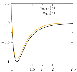
Figure 1: The original KA potential in Eq. (2) and the modified potential in Eq. (3) between species A and A.

Our model is based on the three-dimensional Kob-Andersen binary Lennard-Jones (KALJ) model [34, 35], which has been widely used in the context of the glass transition because of its particularly high glass-forming ability. This model has two types of particles, $A$ and $B$, with a composition ratio of 80:20. Our system is a cubic box with periodic boundary conditions applied in all directions. Both types of particles have the same mass $m$, and the particles interact with each other via a pair potential

$$v_{0,ab}(r)=4\epsilon_{ab}\left[\left(\frac{\sigma_{ab}}{r}\right)^{12}-\left(\frac{\sigma_{ab}}{r}\right)^{6}\right],$$ (2)

where $r$ is the distance between a pair and the parameters are as follows: $\epsilon_{AB}=1.5\epsilon_{AA}$, $\epsilon_{BB}=0.5\epsilon_{AA}$, $\sigma_{AB}=0.8\sigma_{AA}$, and $\sigma_{BB}=0.88\sigma_{AA}$. In this paper, length, mass, and time are reported in units of $\sigma_{AA}$, $m$, and $\sqrt{m\sigma_{AA}^{2}/\epsilon_{AA}}$, respectively. The total number density is fixed at $\rho=1000/(9.4)^{3}\approx 1.204$ [34, 35]. In the KALJ model, Eq. (2) is conventionally cut at a distance $r_{\mathrm{cut},ab}=2.5\sigma_{ab}$. However, the discontinuity of the pair force $v_{0,ab}^{\prime}$ at the cutoff distance strongly affects the low-frequency modes [36]. Thus, we modified Eq. (2) so that its derivative tends to zero continuously

$$v_{ab}(r)=\begin{cases}v_{0,ab}(r)-v_{0,ab}(r_{\mathrm{cut},ab})-(r-r_{\mathrm{cut},ab})v^{\prime}_{0,ab}(r_{\mathrm{cut},ab})&(r<r_{\mathrm{cut},ab}),\\ 0&(r>r_{\mathrm{cut},ab})\end{cases}.$$ (3)

Compare $v_{0,AA}(r)$ and $v_{AA}(r)$ in Fig. 1. Using Eq. (3), we carried out molecular dynamics (MD) simulations. First, the system was equilibrated at a sufficiently high temperature $T=2.0$ in the NVT ensemble for a time interval of $t=500$, and then we performed simulations in the NVE ensemble for the same time interval. At this high temperature, the equilibration time is about unity. Independent liquid configurations were sampled in the subsequent NVE simulation. The time interval between two consecutive configurations is $t=50$. Note that in Sec. III.1.2 we will show the results at much lower temperatures to compare them with the results in Sec. III.1.1. The algorithm for generating these low-temperature samples is explained in detail at the beginning of Sec. III.1.2.

Table 1: The number of samples for each $N$. The number of samples used to plot Figs. 11 and 12 is given in parentheses. See the text for details.

$N$	#samples
1000	1000 (10000)
2000	1000
4000	1000
8000	500
32000	498 (10000)
128000	495

Starting from these liquid states, we performed simulations of the steepest descent dynamics [6, 7]; namely, we numerically solved the following equation of motion:

$$\gamma\derivative{\boldsymbol{r}_{i}}{t}=-\partialderivative{V}{\boldsymbol{r}_{i}},$$ (4)

where $\boldsymbol{r}_{i}$ is the position of particle $i$, and $V=\sum_{i<j}v_{ab}(r_{ij})$ is the total potential energy. The discretized time step was set at $\Delta t=0.0001$ and the friction coefficient $\gamma$ at unity. This dynamics stops at the time when the system reaches an inherent structure, at which $\partialderivative*{V}{\boldsymbol{r}_{i}}=0$ for all $i$, but since our purpose was to investigate transient configurations during the dynamics, we did not need to wait for the system to reach an inherent structure. The number of configurations used for each $N$ is listed in Tab. 1. To plot Figs 11 and 12, we needed a particularly large sample size and the number of configurations is given in the parentheses in Tab. 1. All simulations were performed using Large-scale Atomic/Molecular Massively Parallel Simulator (LAMMPS) [37, 38].

We performed a normal mode analysis [39] of instantaneous configurations during the steepest descent dynamics. The dynamical matrix, the Hessian matrix of the total potential $V$, was diagonalized to obtain its eigenvalues $\lambda_{\alpha}$ and eigenvectors $\boldsymbol{e}_{\alpha}=(\boldsymbol{e}_{\alpha,1},\dots,\boldsymbol{e}_{\alpha,N})$, where $\alpha=1,2,\dots,3N-3$. The three modes corresponding to the global translations were excluded. The eigenvalues are sorted in ascending order: $\lambda_{1}<\lambda_{2}<\dots<\lambda_{3N-3}$, and the eigenvectors are normalized as $|\boldsymbol{e}_{\alpha}|=1$.

III Results

III.1 Mean squared force and fraction of unstable modes

In this subsection we investigate the time evolution of the mean squared force $W$ and the fraction of unstable modes

$$f_{u}=\int_{-\infty}^{0}\differential{\lambda}D(\lambda),$$ (5)

where $D(\lambda)$ is the spectrum, or the density of states, defined as

$$D(\lambda)=\frac{1}{3N-3}\sum_{\alpha=1}^{3N-3}\delta\quantity(\lambda-\lambda_{\alpha}).$$ (6)

As mentioned in the introduction, the mean squared force $W$ is an important quantity to characterize the steepest-descent dynamics and we will first confirm that our results are consistent with the previous results [6, 7] below by using $W$.

However, we emphasize that our main purpose in this subsection is not to determine the detailed time-dependence of $W$, which has been studied intensively in Refs. [6, 7], but to investigate the qualitative relation between $W$ and $f_{u}$. In particular, we verify the prediction in Ref. [4]; namely, the relaxation dynamics after quenching proceeds slowly because the system travels along an almost flat gorge in the potential energy landscape. From $W$ and $f_{u}$, one can estimate the dependence of the potential energy $V$ on $f_{u}$ at long times [1, 11, 40, 19], which is necessary to evaluate the flatness of the potential energy landscape as will be described in the next paragraph.

The $f_{u}$-derivative of the potential energy $\partialderivative*{(V/N)}{f_{u}}$ gives the difference of the potential energy between stationary points with different numbers of unstable modes and has been well studied in terms of saddle modes [41, 1, 11, 40, 19]. We have

$$V_{n+1}-V_{n} =\frac{1}{3N-3}\frac{V_{n+1}-V_{n}}{f_{u,n+1}-f_{u,n}}=\frac{N}{3N-3}\frac{V_{n+1}/N-V_{n}/N}{f_{u,n+1}-f_{u,n}}\xrightarrow{N\to\infty}\frac{1}{3}\partialderivative{(V/N)}{f_{u}},$$ (7)

where $\bullet_{n}$ denotes the value measured at a stationary point with $n$ unstable directions, i.e., modes with negative eigenvalues. The first equality is a consequence of $f_{u,n}=n/(3N-3)$. The derivative in Eq. (7) measures how much energy the system releases when an unstable mode disappears and the system is slightly stabilized. This is the meaning of the flatness, i.e., the smaller this derivative, the flatter the potential energy landscape. Note that, for the rightmost expression in Eq. (7) to be meaningful, we assumed $V_{n+1}-V_{n}=\order{N^{0}}$, which is plausible for finite-dimensional systems because the dynamics is driven by localized modes as will be shown in Sec. III.2. Also, Eq. (7) is strictly justified only for stationary points and should be used as an approximation for instantaneous normal modes. We nevertheless expect that this approximation improves as $t\to\infty$ during the steepest descent dynamics because the system stays close to stationary points for a long time in the last stage of the dynamics [4]. Thus in this section, we investigate the flatness of the potential energy landscape at long times using Eq. (7).

In Sec. III.1.1, we explain the difficulty in computing the ensemble average at a fixed time and introduce an ensemble with a fixed $W$. Then we show high-temperature results at $T=2.0$ and discuss $\partialderivative*{(V/N)}{f_{u}}$ in the limit $t\to\infty$. In Sec. III.1.2, we show the same results at low temperatures.

III.1.1 High temperature

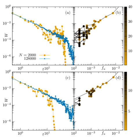
Figure 2: (a, c) Mean squared force $W$ for $N=2000$ and 128000 as functions of the time. (b, d) Mean squared force $W$ versus fraction $f_{u}$ of unstable modes corresponding to the data for $N=2000$ in the panels (a, c). The color bars indicate the time.

We first show raw data at $T=2.0$ in Fig. 2 to introduce the averaging procedure adopted in this study. Figure 2(a) shows the mean squared force $W$ for $N=2000$ and 128000 as functions of the time and Fig. 2(b) is a parametric plot of $W$ versus the fraction of unstable modes $f_{u}$. The data in Fig. 2(b) were taken from the same trajectory of $N=2000$ in Fig. 2(a). In Fig. 2(c, d), we present the same plots for different samples, to be compared in the next paragraph. Although the data in Fig. 2 is noisy, one can see that the mean squared force $W$ first exhibits an almost algebraic decay followed by a precipitous drop at a particular time point. The system finds an inherent structure and the dynamics stops immediately after the drop. For larger $N$, the range of the algebraic decay extends and the convergence to an inherent structure slows down. The fraction of unstable modes decreases with decreasing $W$, but the decay is not monotonic and the value of $f_{u}$ oscillates randomly.

Figure 2 indicates the difficulty in carrying out an ensemble average; because of the strong fluctuations of the time at which $W$ converges to zero, the ensemble average at a fixed time will suffer from significant uncertainties in the late stage. Compare Fig. 2(a,b) and (c,d). In addition, we point out a conceptual problem of the fixed time average. Because of the fluctuations of the convergence time, there is a time interval, in which some samples already converged to inherent structures while the others have not converged yet and are migrating in the potential energy landscape. If we adopt the fixed time average, these two kinds of samples are mixed within this interval. However, they are in physically different states and such mixing may lead to unclear, or possibly incorrect, results because instantaneous normal modes strongly reflect the structure of the potential energy landscape. To avoid these issues, we averaged the data at fixed $W$. During simulations, we sampled a configuration every time $W$ reaches a specific value and averaged observables over configurations with the same $W$.

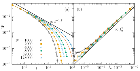
Figure 3: (a) Average mean squared force as functions of the time. The solid line represents a power law $W\propto t^{-1.7}$ [6, 7]. Note that $W$ is controlled in this plot, see the text for details. The errors are smaller than the symbols and thus not shown. (b) Average mean squared force versus fraction of unstable modes. The solid line represents a power law $W\propto f_{u}^{2}$.

Figure 3 shows the same data as in Fig. 2, which are averaged with $W$ fixed. The average mean squared force in Fig. 3(a) decays algebraically and drops mildly at a time depending on the system size $N$. The algebraic decay in the middle stage is compared by a power law $W\propto t^{-1.7}$ [6, 7], as shown by the solid line. Note that this is twice the exponent $\beta=0.85$ reported in Refs. [6, 7] because $\sqrt{W}$ was measured in these studies. Since it is difficult to investigate how the power-law relation $W\sim t^{-1.7}$ breaks down in the late stage of the dynamics for our limited system sizes, understanding this final regime quantitatively is left for future work. Figure 3(b) shows another power law, $W\propto f_{u}^{2}$, which holds down to $W\sim 10^{-8}$. The system approaches a stable inherent structure $W\to 0$ as the fraction of unstable modes $f_{u}$ becomes smaller. It seems that the power law $W\propto f_{u}^{2}$ breaks down slightly in the smallest-$W$ region $W\sim 10^{-8}$. One needs much larger systems to establish the precise functional form $W(f_{u})$ in this region. However, the details of these data will not affect the analysis of the $f_{u}$-derivative of the potential energy described at the beginning of this section. Likewise, the exponents of the power laws observed in Fig. 3 are not generally universal as will be discussed in Sec. III.1.2 (see also Refs. [6, 7]), but the results below do not strongly depend on the values of the exponents.

Related to these results, we note that similar scaling relations were reported for the spherical Sherrington-Kirkpatrick (SK) model [4]. This simple mean-field model does not show a glass transition, but it is characterized by slow relaxation similar to that of the spherical $p$-spin model with $p>2$, which has a spin-glass phase. In Ref. [4], it was shown that $W\sim t^{-2}$ and $f_{u}\sim t^{-3/2}$, which leads to $W\sim f_{u}^{4/3}$ in the spherical SK model.

We apply Eq. (7) to the regime after the power law $W\sim t^{-1.7}$ in Fig. 3(a). From Eq. (4), we have

$$\gamma\quantity|\derivative{(V/N)}{t}|=-\frac{\gamma}{N}\sum_{i=1}^{N}\partialderivative{V}{\boldsymbol{r}_{i}}\derivative{\boldsymbol{r}_{i}}{t}=\frac{1}{N}\sum_{i=1}^{N}\boldsymbol{f}_{i}^{2}=W.$$ (8)

Using the power law $W\propto f_{u}^{2}$, we obtain

$$\partialderivative{(V/N)}{f_{u}}=\frac{\derivative{(V/N)}{t}}{\derivative{f_{u}}{t}}\sim-\frac{W}{\frac{1}{\sqrt{W}}\derivative{W}{t}}=\frac{W^{3/2}}{\quantity|\derivative{W}{t}|}.$$ (9)

As shown in Fig. 3(a), the mean squared force finally decays to zero very fast. For example, one can assume an exponential decay $W(t)\sim e^{-\tau/\tau_{0}}$ or an algebraic decay $W(t)\sim t^{-\upsilon}$ with a sufficiently large exponent $\upsilon>2$. Thus, it is reasonable to assume that $W^{3/2}\ll\quantity|\derivative*{W}{t}|$, which leads to $\partialderivative*{(V/N)}{f_{u}}\xrightarrow{t\to\infty}0$. The fact that the $f_{u}$-derivative of the potential energy tends to zero in the final stage of the dynamics indicates that the potential energy landscape becomes flatter as the system approaches an inherent structure [1] as explained above. This is direct evidence of the almost flat gorge of the potential energy landscape predicted in Ref. [4]. We again emphasize that the details of the functional forms of $W(t)$ and $W(f_{u})$ in Fig. 3 are not relevant unless the value of the limit $\lim_{t\to\infty}\partialderivative*{(V/N)}{f_{u}}$ changes.

To conclude this subsection, we make a remark on the measurement of the potential energy $V$. As seen in the analysis of $\partialderivative*{(V/N)}{f_{u}}$, the most important observable is the potential energy itself rather than the mean squared force $W$. However, the potential energy does not vanish at inherent structures in general and its value $V_{\mathrm{inh}}$ fluctuates while $W$ converges to zero. The measurement of $W$ can be more precise than that of $V$. This is a reason why the $W$-function was chosen in this and related studies [6, 7]. Also, this $W$-function has been used to locate saddle points in the potential energy landscape to verify the prediction of the mode-coupling theory as mentioned in the introduction [10, 42].

III.1.2 Low temperatures

Here, we present the results at low temperatures $T=0.4500$, 0.4308, and 0.3971, which correspond to those in Fig. 3, to investigate how the above results change at sufficiently low temperatures. For $T=0.4500$, equilibrium configurations were prepared by the MD simulations in the NVT ensemble using the Nosé-Hoover thermostat [43]. Starting from configurations equilibrated at $T=2.0$, the MD simulations in the NVT ensemble were performed for $t=10^{5}$, and then we performed simulations in the NVE ensemble for the same time interval. We used time-reversible integrator [44, 43] with a time step of 0.005. The number of samples prepared at this temperature is 1000. To sample the equilibrium configurations at lower temperatures, $T=0.4308$ and 0.3971, we used the replica exchange method [45, 46]. In our MD simulations, 18 replicas were used and each replica corresponded to a temperature ranging from 0.7800 to 0.3971. Exchange trials were performed every 2800 MD steps using the Metropolis criterion. We checked that all replicas were equilibrated after 350000 exchange trials and sampling was performed every 10000 trials thereafter. All calculations were carried out in an in-house code that uses MPI to handle parallel computations of exchanging replicas. Because of the high computational cost, we were only able to prepare 45 samples of $N=1000$.

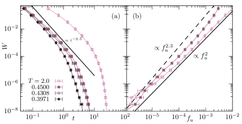
Figure 4: (a) Time evolution of mean squared force from different temperatures $T$. The system size is $N=1000$. The solid line represents a power law $W\propto t^{-2.5}$. (b) Mean squared force versus fraction of unstable modes. The solid and dashed lines represent power law $W\propto f_{u}^{2}$ and $W\propto f_{u}^{2.3}$, respectively.

Using these low-temperature configurations, we performed the same analysis as described in the previous subsection. Figure 4 corresponds to Fig. 3. The solid line in Fig. 4(a) represents a power law $W\propto t^{-2.5}$, which was observed in Ref. [7]. This is not inconsistent with the data, though we cannot verify this power law because of the small system size. Also, it is possible to generalize the discussion of $\partialderivative*{(V/N)}{f_{u}}$. Setting $W\sim f_{u}^{b}$, where $b>0$, yields

$$\partialderivative{(V/N)}{f_{u}}\sim\frac{W^{2-1/b}}{\quantity|\derivative{W}{t}|}.$$ (10)

As shown in Fig. 4(a), $W$ drops similarly to the high-temperature data in Fig. 3(a) in the last stage of the dynamics and thus we conclude that $\partialderivative*{(V/N)}{f_{u}}\xrightarrow{t\to\infty}0$. Larger systems are necessary to establish this result.

In summary, the data in Figs. 3 and 4 indicate that the system moves on an almost flat gorge of the potential energy landscape at long times, which is consistent with the results of mean-field models in Ref. [4]. This result does not strongly depend on the precise functional forms of $W(t)$ and $W(f_{u})$, which may not be universal. In Appendix E, we will show the corresponding results for weakly jammed solids and confirm that $\lim_{t\to\infty}\partialderivative*{(V/N)}{f_{u}}=0$, though the specific exponents of the power laws change.

III.2 Spectrum and localization

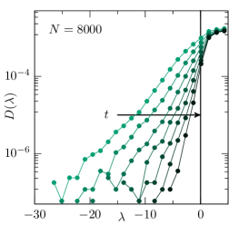
Figure 5: Unstable parts of the spectra for $N=8000$ during the dynamics. The values of the mean squared force are $\log_{10}W=-4.5,-4.0,-3.5,-3.0,-2.5,-2.0$, and $-1.5$ from right to left. The arrow indicates the direction of time, which is the opposite of $W$.

The spectrum $D(\lambda)$ in Eq. (6) is a fundamental quantity for characterizing stationary points of the potential energy landscape. Though Figs. 2 and 3 show an integrated version of it, $f_{u}$, direct investigation of the spectrum gives more insight into the dynamics. In this subsection, we also investigate the degree of localization of unstable modes and show that all unstable modes are localized at long times, which is consistent with the fact that the relaxation dynamics is governed by spatially localized hot spots [6, 7].

Figure 5 shows unstable parts of the spectra for $N=8000$ during the dynamics. As in Sec. III.1, each spectrum is labeled by the value of $W$ and the specific values are $\log_{10}W=-4.5,-4.0,-3.5,-3.0,-2.5,-2.0$, and $-1.5$ from right to left. Note that, however, the arrow in Fig. 5 indicates the direction of time, which is the opposite of $W$. In Appendix A, we will confirm that the spectrum does not depend on the system size $N$. From Fig. 5, one can see that the unstable part of the spectrum always shows an exponential tail.

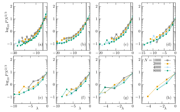
Figure 6: $\log_{10}PN^{2/3}$ versus $\lambda$. The values of $\log_{10}W$ are (a) $-1.5$, (b) $-2$, (c) $-2.5$, (d) $-3$, (e) $-3.5$, (f) $-4$, (g) $-4.5$, and (h) $-5$. For panels (a), (b), (c), and (d), the estimated mobility edges are shown by the solid lines.

The exponential tail of the spectrum is a characteristic of localized modes found at saddle points [42]. The level spacing distribution of such localized modes is a Poisson distribution, which means that these eigenvalues are uncorrelated with each other [42]. These saddle modes are truly localized, meaning that their particle motions strongly decay far from the localized cores, while the quasi-localized modes found at inherent structures have algebraically decaying far fields and its density follows a quartic law $g(\omega^{4})=\omega D(\omega^{2})\propto\omega^{4}$, where $\omega=\sqrt{\lambda}$ is the frequency [25, 26]. Thus it is important to understand the degree of localization of the unstable modes observed in Fig. 5. This motivated us to perform a finite-size scaling analysis of the participation ratio [47, 48, 49]

$$P_{\alpha}=\frac{1}{N}\left(\sum_{i=1}^{N}|\boldsymbol{e}_{\alpha,i}|^{4}\right)^{-1},$$ (11)

which measures the degree of localization of a given mode $\alpha$. If all particles vibrate equally, $P_{\alpha}=1$ and if only a single particle vibrates, $P_{\alpha}=1/N$. Thus, $NP_{\alpha}$ gives the number of particles participating in the mode, enabling us to determine the mobility edge $\lambda_{e}$, which separates localized and delocalized modes. Specifically, the average participation ratio $NP=N\langle P_{\alpha}\rangle_{\lambda}$ at $\lambda$, for delocalized modes grows at least linearly with $L$, where $L$ is the linear size of the system, whereas it is independent of $L$ for localized modes [50, 42]. Namely, delocalized modes expand throughout the system at least in a direction. Thus, the mobility edge, the border between these two species of modes, is defined as a fixed point of $NP/L\propto NP/N^{1/3}=N^{2/3}P$, by changing $N$ [50, 42]. Figure 6 shows $N^{2/3}P$ as functions of the eigenvalue $\lambda$ and the values of $\log_{10}W$ are (a) $-1.5$, (b) $-2$, (c) $-2.5$, (d) $-3$, (e) $-3.5$, (f) $-4$, (g) $-4.5$, and (h) $-5$. We will show scatter plots of $PN^{2/3}$ versus $\lambda$ in Appendix B. The mobility edge, estimated as the mean intersection of pairs of data for different $N$, is shown by the solid line in each of Fig 6(a–d). Figure 6 shows that the modes are localized for $\lambda<\lambda_{e}$ and delocalized for $\lambda>\lambda_{e}$. It can be seen that the mobility edge converges to zero $\lambda_{e}\to 0$ long before the system falls into an inherent structure. See also Fig. 7, in which we plot the mobility edge as a function of $W$. This result suggests that all unstable modes are localized during most of the relaxation process in the limit $N\to\infty$; namely, localized modes dominate the dynamics. Note that the mobility edge cannot be positive because of the phonons that are always delocalized. To further corroborate this result, it is helpful to compute the level spacing distribution [18, 21, 42], although the number of samples used in this study is too small to obtain precise data, particularly for small $W$.

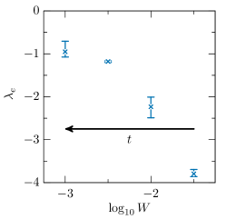
Figure 7: Mobility edge as a function of $W$. The arrow indicates the direction of time, which is the opposite of $W$. The errors are estimated as minimum and maximum values of the intersections of pairs of data for different $N$ in Fig. 6.

III.3 The most unstable mode

In Sec. III.2, we found that the steepest descent dynamics is controlled mostly by unstable localized modes. Here we focus on the most unstable mode, which is the most localized. The most unstable mode of a configuration is often well isolated from the other modes [25, 51, 33] and thus one can extract characteristics of localized modes cleanly. We investigate the time evolution of the most unstable mode and how it is stabilized. Obviously, the most unstable mode is the last unstable mode to disappear and thus its understanding gives us insight into what happens in the late stage of the dynamics.

III.3.1 Decay profile and correlation length

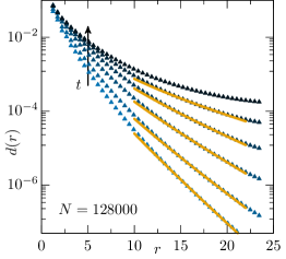
Figure 8: Decay profiles for $N=128000$. The values of $W$ are $\log_{10}W=-7$, $-6$, $-5$, $-4$, $-3$, and $-2$ from top to bottom. The arrow indicates the direction of time. The errors are smaller than the symbols and thus not shown. The solid lines indicate Eq. (12).

First, we consider the decay profile $d(r)$ [52, 25]. It quantifies how an eigenvector decays from its localized core, defined as the particle with the largest norm (see Appendix C for the detailed definition). Figure 8 shows the decay profiles of the most unstable modes for $N=128000$ at several values of $W$. As in Fig. 5, the arrow shows the direction of time, which is the opposite of $W$. We present the corresponding data for $N=8000$ and 32000 in Appendix A to examine the system size dependence. In the early stage of the dynamics, or the large-$W$ regime, the profile decays exponentially with distance $r$ from the core. This behavior resembles that of unstable localized modes found at saddle points [33]. As $W$ decreases with time, this decay becomes slower and the far field develops.

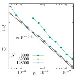
Figure 9: The logarithm of the correlation length $\ln\xi$ as a function of the mean squared force $W$. The solid line represents a stretched exponential law $\ln\xi\propto W^{-0.11}$.

In the case of inherent structures, the lowest-frequency modes are quasi-localized and it has been pointed out that they resemble the elastic response to a local dipolar force [53, 27, 54], which is the gradient of Green’s function, or the displacement correlation function, of an elastic medium [55]. This fact motivates us to fit the decay profiles in Fig. 8 using Green’s function. Since one cannot directly use Green’s function of an elastic medium to fit the data of non-equilibrium transient states during the relaxation dynamics, we tentatively assume that Green’s function is written in the simplest form $G(r)\sim e^{-r/\xi}/r$, where $\xi$ is the correlation length [56]. Then the decay profile is expected to follow

$$d(r)\sim\quantity|\partialderivative{r}G(r)|\sim\quantity(\frac{1}{r^{2}}+\frac{1}{\xi r})e^{-r/\xi}.$$ (12)

As will be seen below, the correlation length diverges in the long-time limit $\xi\xrightarrow{t\to\infty}\infty$. This is consistent with the result of inherent structures $d_{\mathrm{inh}}(r)\sim 1/r^{2}$, which corresponds to the elastic field of Eshelby inclusion [27]. Thus so to speak, the system behaves like a solid for $r\ll\xi$ and a liquid for $r\gg\xi$.

We fitted Eq. (12) to the data in Fig. 8, see the solid lines. Although the fitting was performed over a range of $r\in[15,20]$, the solid lines are shown over a larger range of $r\in[10,22]$. We plotted the logarithm of the correlation length $\ln\xi$ as a function of the mean squared force $W$ for $N=8000$, 32000, and 128000 in Fig. 9. The data depend on the system size, but appear to converge rapidly as $N\to\infty$ except for the smallest-$W$ regime, $W\sim 10^{-7}$. Larger systems are necessary to investigate this regime. For all $N$, $\xi$ diverges as $W\to 0$, or $t\to\infty$, and it obeys a stretched exponential law $\xi\propto e^{W^{-0.11}}$ over four decades in $W$ for $N=128000$. This simply means that the solid-like region expands during the relaxation process. However, this non-trivial time dependence has not been reported in the context of relaxation dynamics, at least to our knowledge, and its underlying mechanism remains to be explored in future work.

III.3.2 Energy profile and its statistics

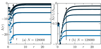
Figure 10: (a) Energy profiles for $N=128000$. The values of $W$ are $\log_{10}W=-7$, $-6$, $-5$, $-4$, $-3$, and $-2$ from top to bottom. The arrow indicates the direction of time. (b) Energy profiles normalized by the minimum values $\Lambda_{\mathrm{min}}$.

It is possible to investigate the local mechanical stability based on the spatial distribution of the eigenenergies of unstable modes. Thus, we next study the energy profile $\Lambda(r)$ [51, 33, 57] of the most unstable mode. It is a function of the distance $r$ from the particle that has the most negative local harmonic energy $\delta E_{i}$ for a given mode [51]. Note that the total sum of the local energies is equal to the eigenenergy $\lambda=\sum_{i}\delta E_{i}$. The particle with the most negative local energy usually has the largest norm and thus it can also be understood as a core. Also, the data in Appendix D suggest that the most unstable mode of each configuration has only a single core in terms of the local energy. The energy profile $\Lambda(r)$ is the partial harmonic energy of a mode integrated from the core to the distance $r$. In other words, $\Lambda(r)$ is the harmonic energy that the mode would have if the system were cut at a distance $r$ from the core, and $\Lambda(r\to\infty)$ converges to the eigenvalue of the mode (see Appendix C for the detailed definition).

Figure 10 presents the results for $N=128000$ at the same values of $W$ as in Fig. 8. Figure 10(a) shows the average energy profile of the most unstable modes. Roughly speaking, the overall shape of the profile does not change within this range of $W$ and it only shifts upward as a whole with decreasing $W$. It starts from a negative value by definition, reaches a minimum $\Lambda_{\mathrm{min}}$, shows an upturn, and finally converges to the average eigenenergy. The length at which the energy profile reaches its minimum $\Lambda_{\mathrm{min}}$ is a useful definition of the localization length. The unstable localized modes are interpreted as defects with the energy scale $\Lambda_{\mathrm{min}}$, similar to the modes observed in saddle configurations [42, 33]. Figure 10(a) indicates that the localization length of the most unstable mode is determined in the early stage of the dynamics. This behavior should be compared with the results in Ref. [6], that is, the size of the hot spots increases with time. Probably non-affine displacements in a hot spot involve surrounding particles and thus its size appears to grow in the late stage because the surrounding far field develops as shown in Fig. 8.

Also, one can see that the core and far field evolve on different timescales. Figure 10(b) shows the energy profile normalized by the minimum value $|\Lambda_{\mathrm{min}}|$. While the data with different $W$ almost collapse around the origin, they shift upward far from it. Thus, the far field of the most unstable mode is stabilized more rapidly than the core.

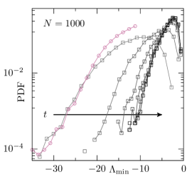
Figure 11: PDFs of $\Lambda_{\mathrm{min}}$ shown by the black squares for $N=1000$. The values of $W$ are $\log_{10}W=-9$, $-7.5$, $-6$, $-4.5$, $-3$, and $-1.5$ from right to left. The arrow indicates the direction of time. The shifted spectrum $100D(\lambda+15.5)$ for $\log_{10}W=-1.5$ is also shown by the pink circles.

Finally, we analyze the core energy $\Lambda_{\mathrm{min}}$ in detail. Figure 11 shows the probability distribution functions (PDFs) of $\Lambda_{\mathrm{min}}$ for $N=1000$ by the black squares. For large values of $W$, the function shows a clear exponential tail. In particular, the shifted spectrum $100D(\lambda+15.5)$ for $\log_{10}W=-1.5$, indicated by the pink circles, almost collapses onto the corresponding data; the functional form of $D(\lambda)$ is almost determined by the statistics of the core energy $\Lambda_{\mathrm{min}}$ and the far field only shifts the spectrum. For small values of $W$, the PDF still appears to decay exponentially. This should be contrasted with the PDF of the eigenvalues of the lowest-frequency quasi-localized modes of inherent structures, which perfectly obeys a Weibull distribution with a power law $g(\omega)\propto\omega^{4}$ [25, 26, 27].

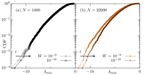
Figure 12: CDFs of $\Lambda_{\mathrm{min}}$ for (a) $N=1000$ and (b) 32000. The arrows indicate the direction of time.

To precisely determine the PDF of the core energy $\Lambda_{\mathrm{min}}$ for small $W$, we computed its cumulative distribution function (CDF), which is free from the binning error unlike the PDF. Figure 12 shows the CDFs of $\Lambda_{\mathrm{min}}$ for (a) $N=1000$ and (b) $N=32000$. The values of $W$ are $10^{-9}$ and $10^{-16}$. These values of $W$ are very small and the system of $W=10^{-16}$ has no unstable modes, i.e., it is an inherent structure. For any $N$ and $W$, the CDF exhibits an exponential tail. Figures 11 and 12 show that the distribution of $\Lambda_{\mathrm{min}}$ remains exponential, whereas that of the eigenenergy $\lambda=\Lambda(r\to\infty)$ gradually develops an algebraic tail [25, 26, 27]. For small $W$, the far field essentially contributes to the statistics of the localized modes while it only shifts the spectrum in the large-$W$ regime.

IV Summary and conclusion

In this paper, we numerically studied the steepest descent dynamics as one of the simplest models of quenching. We focused on unstable normal modes of instantaneous configurations during the dynamics and investigated how their statistics and spatial structure change toward mechanically stable final configurations called inherent structures.

In Sec. III.1, we examined the time evolution of the mean squared force $W$ and the fraction of unstable modes $f_{u}$. We compared our data with power laws $W\propto t^{-1.7}$ [6, 7] and $W\propto f_{u}^{2}$ at a sufficiently high temperature $T=2.0$. These data lead to the vanishing $f_{u}$-derivative of the total potential energy, $\partialderivative*{(V/N)}{f_{u}}\xrightarrow{t\to\infty}0$, meaning that paths in the potential energy landscape passed by quenched liquids become flatter as the dynamics proceeds, i.e., the system moves on a gorge [4]. The same analysis of low-temperature configurations revealed that the value of the limit $\lim_{t\to\infty}\partialderivative*{(V/N)}{f_{u}}$ does not change.

The results in Sec. III.1 are intimately related to the notion of marginal stability [58, 59, 60], which assumes an increasingly important role in understanding anomalous behavior of glasses. The marginal stability of amorphous materials is often characterized by the flat free energy landscape predicted by replica theory as full replica symmetry breaking [59, 60]. In terms of mechanical stability, marginally stable systems have low-energy excitations with a gapless spectrum and are extremely susceptible to perturbations [58]. Thus the observed flatness of the potential energy landscape strongly calls for the investigation of other related properties of marginal stability during the relaxation dynamics after quenching.

In Sec. III.2, we found that the spectrum of unstable normal modes exhibits an exponential tail, a known characteristic of localized modes at saddle points [42]. Performing a finite-size scaling analysis, we located the mobility edge, which appears to converge to zero long before the system falls into an inherent structure. Thus, the motion of the particles is mainly governed by localized modes in the late stage of the dynamics. This finding is consistent with the previous studies [6, 7].

In Sec III.3, we focused on the most unstable modes of instantaneous configurations and investigated how their structure develops during the relaxation process. The decay and energy profiles revealed that the core length of these modes is already determined in the early stage of the dynamics. In contrast, the surrounding far field significantly develops during the dynamics with the correlation length $\xi$, which separates the solid-like and liquid-like regimes. The correlation length diverges with a non-trivial stretched exponential law $\ln\xi\propto W^{0.11}$. Moreover, the PDF of the core energy $\Lambda_{\mathrm{min}}$ remains exponential in contrast to the power-law distribution of the smallest eigenvalues of inherent structures [25, 26, 27]. These results mean that the cores of the quasi-localized modes are hot spots left to be unstable during the dynamics while the overall system is rapidly stabilized. The results in Sec. III.2 and III.3 indicate that standard methods of normal mode analysis are quite effective to investigate hot spots, which were originally defined by directly observing particle displacements [6, 7].

To the best of our knowledge, many of the results reported in this paper, such as the stretched exponential law of the correlation length $\xi$, have not been observed in previous studies of the relaxation dynamics and no theory predicts them. It would be interesting to study whether several theoretical models such as the elastoplastic model discussed in Refs. [61, 62, 63, 64] can reproduce them. Also, it would be worth investigating different quenching algorithms such as the conjugate gradient method or fast inertial relaxation engine [65]. Although most studies [6, 7], including this work, have focused on the steepest descent dynamics, which is the overdamped Langevin equation, realistic systems often have inertia and their relaxation dynamics can be modeled as those other algorithms. Since different algorithms lead to different inherent structures even if the system starts from the same initial state [7], it might be the case that some of the results in this paper are modified. It is then possible to classify the non-equilibrium relaxation dynamics after quenching.

Conflicts of interest

There are no conflicts of interest to declare.

Appendix A System size dependence

We examine the system size dependence of the spectrum, decay profile, and energy profile. Figure 13 shows the spectra for $N=1000$, 2000, 4000, and 8000 at several values of $W$. In Figs. 14 and 15, we show the decay profiles for $N=8000$ and 32000 corresponding to Fig. 8. In Figs. 16 and 17, we show the energy profiles for $N=8000$ and 32000 corresponding to Fig. 10. From these figures, it is evident that the data do not qualitatively depend on the system size.

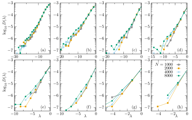
Figure 13: Unstable parts of the spectra for $N=1000$, 2000, 4000, and 8000. The values of $\log_{10}W$ are (a) $-1.5$, (b) $-2$, (c) $-2.5$, (d) $-3$, (e) $-3.5$, (f) $-4$, (g) $-4.5$, and (h) $-5$.

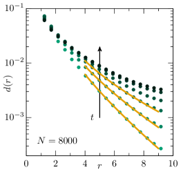
Figure 14: Decay profiles for $N=8000$. The values of $W$ are $\log_{10}W=-7$, $-6$, $-5$, $-4$, $-3$, and $-2$ from top to bottom. The arrow indicates the direction of time. The errors are smaller than the symbols and thus not shown. The solid lines indicate Eq. (12). The fitting was performed over a range of $r\in[5,8]$, but the solid lines are shown over a larger range of $r\in[4,9]$.

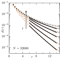
Figure 15: Decay profiles for $N=32000$. The values of $W$ are $\log_{10}W=-7$, $-6$, $-5$, $-4$, $-3$, and $-2$ from top to bottom. The arrow indicates the direction of time. The errors are smaller than the symbols and thus not shown. The solid lines indicate Eq. (12). The fitting was performed over a range of $r\in[8,12]$, but the solid lines are shown over a larger range of $r\in[6,14]$.

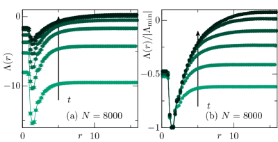
Figure 16: (a) Energy profiles for $N=8000$. The values of $W$ are $\log_{10}W=-7$, $-6$, $-5$, $-4$, $-3$, and $-2$ from top to bottom. The arrow indicates the direction of time. (b) Energy profiles normalized by the minimum values $\Lambda_{\mathrm{min}}$.

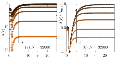
Figure 17: (a) Energy profiles for $N=32000$. The values of $W$ are $\log_{10}W=-7$, $-6$, $-5$, $-4$, $-3$, and $-2$ from top to bottom. The arrow indicates the direction of time. (b) Energy profiles normalized by the minimum values $\Lambda_{\mathrm{min}}$.

Appendix B Raw data for the participation ratio

Figure 18 shows raw data corresponding to Fig. 6(a–d). We show the data of a single sample for each $N$ and $W$. The data points look quite scattered, but one can obtain clean data by averaging over a large number of samples as in Fig. 6

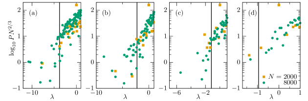
Figure 18: Raw data corresponding to Fig. 6. The solid lines indicate the mobility edges defined in Sec. III.2.

Appendix C Definitions of decay and energy profiles

We give the detailed definitions of the decay and energy profiles introduced in Sec. III.3.

C.1 Decay profile

The decay profile [25, 52] $d(r)$ of a mode $\boldsymbol{e}$ is a function of the distance $r$ from the particle with the largest norm $|\boldsymbol{e}_{i}|$, the position of which is denoted by $\boldsymbol{r}_{d}$. It is defined as

$$d(r)=\underset{\begin{subarray}{c}i\\ |\boldsymbol{r}_{i}-\boldsymbol{r}_{d}|\in[r-\Delta r/2,r+\Delta r/2]\end{subarray}}{\operatorname{median}}|\boldsymbol{e}_{i}|,$$ (13)

where $\Delta r$ is the bin width. The distance $r$ used here differs slightly from the one in the original paper by Gartner and Lerner [52]. They defined the center of an eigenmode using $w$ particles with the largest norms and measured the distance $r$ from this center. They mainly used $w=4$ while our definition corresponds to $w=1$. However, this difference does not affect the results qualitatively in the case of spatially localized modes.

C.2 Energy profile

The local vibrational energy of the $i$-th particle in a mode $\boldsymbol{e}$ is

$$\delta E_{i} =\frac{1}{2}\sum_{j=1}^{N}\left[v^{\prime\prime}_{ij}(r_{ij})(\boldsymbol{n}_{ij}\cdot\boldsymbol{e}_{ij})^{2}+\frac{v^{\prime}_{ij}(r_{ij})}{r_{ij}}(\boldsymbol{e}_{ij}^{\perp})^{2}\right],$$ (14)

where $\boldsymbol{n}_{ij}$ is the unit vector pointing from $i$ to $j$, $\boldsymbol{e}_{ij}=\boldsymbol{e}_{i}-\boldsymbol{e}_{j}$ is the relative displacement between the pair, and $(\boldsymbol{e}_{ij}^{\perp})^{2}=(\boldsymbol{e}_{ij})^{2}-(\boldsymbol{n}_{ij}\cdot\boldsymbol{e}_{ij})^{2}$ is the squared transverse relative displacement. The energy profile [51] $\Lambda(r)$ is a function of the distance $r$ from the particle with the most negative $\delta E_{i}$, the position of which is denoted by $\boldsymbol{r}_{e}$. It is defined as

$$\Lambda(r) =\sum_{i=1}^{N}\Theta(r-|\boldsymbol{r}_{i}-\boldsymbol{r}_{e}|)\delta E_{i}=\int_{|\boldsymbol{x}|<r}d\boldsymbol{x}\delta E(\boldsymbol{x}),$$ (15)

where $\Theta(x)$ is the Heaviside step function. In the rightmost expression, we rewrote the function using a spatial integral of the local energy density $\delta E(\boldsymbol{r})=\sum_{i}\delta E_{i}\delta[\boldsymbol{r}-(\boldsymbol{r}_{i}-\boldsymbol{r}_{e})]$. Thus, the energy profile is the vibrational energy that the mode would have if the system was cut at a distance $r$ from the center $\boldsymbol{r}_{e}$. It converges to the eigenvalue of the mode $\lambda$ as $r\to\infty$. Finally, note that the difference between $\boldsymbol{r}_{d}$ and $\boldsymbol{r}_{e}$ does not matter in practice because they usually coincide [51].

Appendix D Number of cores

We show data that suggest that there is a single core in the most unstable mode of each configuration on average. By the term “core”, we mean the particle with the most negative harmonic energy $\delta E_{i}$. In this appendix, the particles are sorted in the ascending order of $\delta E_{i}$, i.e., $\delta E_{1}<\delta E_{2}<\cdots$. In Fig. 19, the average distance from the core $r_{i}$ is plotted against the average harmonic energy $\delta E_{i}$ for several values of $W$ indicated by the colors. Each panel shows only the data for the ten particles with the most negative harmonic energies for each $W$. This figure indicates that these unstable particles are close to the core particles $i=1$ and thus, it is unlikely that they constitute other independent cores.

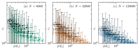
Figure 19: The average distance from the core $r_{i}$ versus the harmonic energy $\delta E_{i}$ for (a) $N=8000$, (b) 32000, and (c) 128000. The error bar indicates the standard deviation of each data point and not the error itself. The values of $W$ are $\log_{10}W=-2$, $-3$, $-4$, $-5$, $-6$, and $-7$ from light to dark colors.

Appendix E Weakly jammed packings

We investigate instantaneous normal modes of weakly jammed packings during the relaxation dynamics after quenching for comparison with the results of the KALJ model in the main text. This system is composed of monodisperse athermal particles with mass $m$ interacting via a purely repulsive potential. Here we adopted a harmonic potential

$$v(r)=\frac{\epsilon}{2}\quantity(1-\frac{r}{\sigma})^{2}\Theta\quantity(1-\frac{r}{\sigma}).$$ (16)

In this section, length, mass, and time are reported in units of $\sigma$, $m$, and $\sqrt{m\sigma^{2}/\epsilon}$, respectively. The packing fraction is fixed at the same value $\phi=0.73$ as in Ref. [7]. Starting from random configurations, which are equivalent to infinite-temperature states, we performed simulations of the steepest descent dynamics in Eq. (4). We repeated some of the analysis in the main text. The number of configurations used for each $N$ is listed in Tab. 2.

Table 2: The number of samples for each $N$.

$N$	#samples
2000	1000
8000	500
32000	200
128000	100

E.1 Mean squared force and fraction of unstable modes

Figure 20 corresponds to Fig. 3. One can observe power laws $W\propto t^{-1.7}$ and $W\propto f_{u}^{2.3}$. The former is already known [6, 7]. Although the exponent of the latter power law is different from those of the KALJ model, it is easy to repeat the same discussion in Sec. III.1, which leads to

$$\partialderivative{(V/N)}{f_{u}}\xrightarrow{t\to\infty}0.$$ (17)

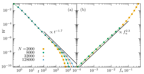
Figure 20: (a) Average mean squared force as functions of the time. The solid line represents a power law $W\propto t^{-1.7}$ [6, 7]. Note that $W$ is controlled in this plot. See the text for details. The errors are smaller than the symbols and thus not shown. (b) Average mean squared force versus fraction of unstable modes. The solid line represents a power law $W\propto f_{u}^{2.3}$.

E.2 Spectrum and localization

Figures 21 and 22 correspond to Figs. 5 and 6, respectively. Although we did not compute the mobility edge, it is obvious from Fig. 22 that the delocalized modes gradually disappear.

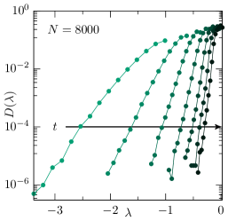
Figure 21: Unstable parts of the spectra for $N=8000$ during the dynamics. The values of the mean squared force are $\log_{10}W=-4.5,-4.0,-3.5,-3.0,-2.5,-2.0$, and $-1.5$ from right to left. The time is indicated by the arrow, which is the opposite of $W$.

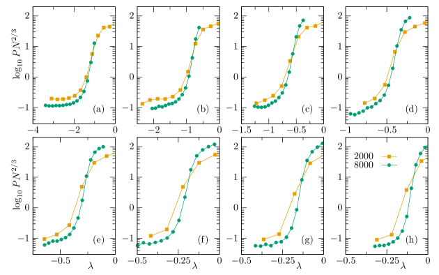
Figure 22: $\log_{10}PN^{2/3}$ versus $\lambda$. The values of $\log_{10}W$ are (a) $-1.5$, (b) $-2$, (c) $-2.5$, (d) $-3$, (e) $-3.5$, (f) $-4$, (g) $-4.5$, and (h) $-5$.

E.3 The most unstable mode

Figures 23, 24, and 25 correspond to Figs. 8, 9, and 10, respectively. In general, the behavior of these functions is qualitatively the same as that for the KALJ model, but the decay profile decays more rapidly in the early stage of the dynamics, or the large-$W$ regime. As a result, the correlation length becomes shorter and does not obey the stretched exponential law $\ln\xi\propto W^{0.10}$ for large $W$. A possible explanation is that a contact network of particles does not percolate in this early stage; namely, the system is composed of small clusters of particles. Such states are not possible in systems with long-range interactions including the KALJ model.

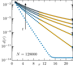
Figure 23: Decay profiles for $N=128000$. The values of $W$ are $\log_{10}W=-10$, $-9$, $-8$, $-6$, $-4$, and $-2$ from top to bottom. The arrow indicates the direction of time. The errors are smaller than the symbols and thus not shown. The solid lines indicate Eq. (12). The fitting was performed over a range of $r\in[15,20]$, but the solid lines are shown over a larger range of $r\in[10,22]$.

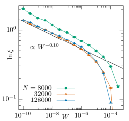
Figure 24: The logarithm of the correlation length $\ln\xi$ as a function of the mean squared force $W$. The solid line represents a stretched exponential law $\ln\xi\propto W^{-0.10}$.

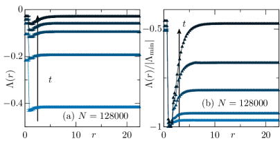
Figure 25: (a) Energy profiles for $N=128000$. The values of $W$ are $\log_{10}W=-10$, $-9$, $-8$, $-6$, and $-4$ from top to bottom. The arrow indicates the direction of time. (b) Energy profiles normalized by the minimum values $\Lambda_{\mathrm{min}}$.

E.4 System size dependence

Figures 26, 27, 28, 29, and 30 correspond to Figs. 13, 14, 15, 16, and 17, respectively. One can see that the data do not depend on the system size qualitatively.

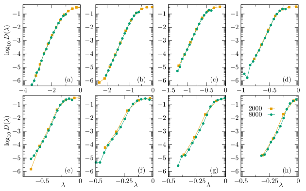
Figure 26: Unstable parts of the spectra for $N=2000$ and 8000. The values of $\log_{10}W$ are (a) $-1.5$, (b) $-2$, (c) $-2.5$, (d) $-3$, (e) $-3.5$, (f) $-4$, (g) $-4.5$, and (h) $-5$.

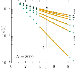
Figure 27: Decay profiles for $N=8000$. The values of $W$ are $\log_{10}W=-10$, $-9$, $-8$, $-6$, $-4$, and $-2$ from top to bottom. The arrow indicates the direction of time. The errors are smaller than the symbols and thus not shown. The solid lines indicate Eq. (12). The fitting was performed over a range of $r\in[5,7.5]$, but the solid lines are shown over a larger range of $r\in[4,8]$.

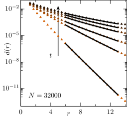
Figure 28: Decay profiles for $N=32000$. The values of $W$ are $\log_{10}W=-10$, $-9$, $-8$, $-6$, $-4$, and $-2$ from top to bottom. The arrow indicates the direction of time. The errors are smaller than the symbols and thus not shown. The solid lines indicate Eq. (12). The fitting was performed over a range of $r\in[8,12]$, but the solid lines are shown over a larger range of $r\in[6,13]$.

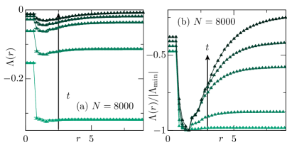
Figure 29: (a) Energy profiles for $N=8000$. The values of $W$ are $\log_{10}W=-10$, $-9$, $-8$, $-6$, and $-4$ from top to bottom. The arrow indicates the direction of time. (b) Energy profiles normalized by the minimum values $\Lambda_{\mathrm{min}}$.

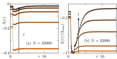
Figure 30: (a) Energy profiles for $N=32000$. The values of $W$ are $\log_{10}W=-10$, $-9$, $-8$, $-6$, and $-4$ from top to bottom. The arrow indicates the direction of time. (b) Energy profiles normalized by the minimum values $\Lambda_{\mathrm{min}}$.

References

- Cavagna [2009] A. Cavagna, Phys. Rep. 476, 51 (2009), arXiv:0903.4264 [cond-mat] .
- Berthier and Biroli [2011] L. Berthier and G. Biroli, Rev. Mod. Phys. 83, 587 (2011), arXiv:1011.2578 [cond-mat] .
- Cugliandolo and Kurchan [1993] L. F. Cugliandolo and J. Kurchan, Phys. Rev. Lett. 71, 173 (1993), arXiv:cond-mat/9303036 .
- Kurchan and Laloux [1996] J. Kurchan and L. Laloux, J. Phys. A: Math. Gen. 29, 1929 (1996), arXiv:cond-mat/9510079 .
- Kob et al. [2000] W. Kob, J.-L. Barrat, F. Sciortino, and P. Tartaglia, Journal of Physics: Condensed Matter 12, 6385 (2000).
- Chacko et al. [2019] R. N. Chacko, P. Sollich, and S. M. Fielding, Phys. Rev. Lett. 123, 108001 (2019), arXiv:1903.00991 [cond-mat] .
- Nishikawa et al. [2022] Y. Nishikawa, M. Ozawa, A. Ikeda, P. Chaudhuri, and L. Berthier, Phys. Rev. X 12, 021001 (2022), arXiv:2106.01755 [cond-mat] .
- González-López and Lerner [2020] K. González-López and E. Lerner, The Journal of Chemical Physics 153, 241101 (2020), arXiv:2010.07153 [cond-mat] .
- Folena et al. [2021] G. Folena, S. Franz, and F. Ricci-Tersenghi, Journal of Statistical Mechanics: Theory and Experiment 2021, 033302 (2021), arXiv:2007.07776 [cond-mat] .
- Angelani et al. [2000] L. Angelani, R. Di Leonardo, G. Ruocco, A. Scala, and F. Sciortino, Phys. Rev. Lett. 85, 5356 (2000), arXiv:cond-mat/0007241 .
- Broderix et al. [2000] K. Broderix, K. K. Bhattacharya, A. Cavagna, A. Zippelius, and I. Giardina, Phys. Rev. Lett. 85, 5360 (2000), arXiv:cond-mat/0007258 .
- Argon [1979] A. Argon, Acta Metallurgica 27, 47 (1979).
- Falk and Langer [1998] M. L. Falk and J. S. Langer, Phys. Rev. E 57, 7192 (1998).
- Tanguy et al. [2006] A. Tanguy, F. Leonforte, and J.-L. Barrat, The European Physical Journal E 20, 355 (2006).
- Schall et al. [2007] P. Schall, D. A. Weitz, and F. Spaepen, Science 318, 1895 (2007).
- Folena et al. [2020] G. Folena, S. Franz, and F. Ricci-Tersenghi, Phys. Rev. X 10, 031045 (2020), arXiv:1903.01421 [cond-mat] .
- Seeley and Keyes [1989] G. Seeley and T. Keyes, The Journal of Chemical Physics 91, 5581 (1989).
- Ciliberti and Grigera [2004] S. Ciliberti and T. S. Grigera, Phys. Rev. E 70, 061502 (2004), arXiv:cond-mat/0404469 .
- Grigera [2006] T. S. Grigera, The Journal of Chemical Physics 124, 064502 (2006), arXiv:cond-mat/0509301 .
- Widmer-Cooper et al. [2009] A. Widmer-Cooper, H. Perry, P. Harrowell, and D. R. Reichman, J. Chem. Phys. 131, 194508 (2009), arXiv:0907.0222 [cond-mat] .
- Clapa et al. [2012] V. I. Clapa, T. Kottos, and F. W. Starr, J. Chem. Phys. 136, 144504 (2012), arXiv:1103.4113 [cond-mat] .
- Palyulin et al. [2018] V. V. Palyulin, C. Ness, R. Milkus, R. M. Elder, T. W. Sirk, and A. Zaccone, Soft Matter 14, 8475 (2018), arXiv:1711.10597 [cond-mat] .
- Oyama et al. [2021] N. Oyama, H. Mizuno, and A. Ikeda, Phys. Rev. Lett. 127, 108003 (2021), arXiv:2011.12568 [cond-mat] .
- Donati et al. [2000] C. Donati, F. Sciortino, and P. Tartaglia, Phys. Rev. Lett. 85, 1464 (2000).
- Lerner et al. [2016] E. Lerner, G. Düring, and E. Bouchbinder, Phys. Rev. Lett. 117, 035501 (2016), arXiv:1604.05187 [cond-mat] .
- Mizuno et al. [2017] H. Mizuno, H. Shiba, and A. Ikeda, Proc. Natl. Acad. Sci. USA 114, E9767 (2017), arXiv:1703.10004 [cond-mat] .
- Lerner and Bouchbinder [2021] E. Lerner and E. Bouchbinder, arXiv:2108.13859 (2021).
- Maloney and Lemaitre [2006] C. E. Maloney and A. Lemaitre, Phys. Rev. E 74, 016118 (2006), arXiv:cond-mat/0510677 .
- Tanguy et al. [2010] A. Tanguy, B. Mantisi, and M. Tsamados, Europhys. Lett. 90, 16004 (2010).
- Manning and Liu [2011] M. L. Manning and A. J. Liu, Phys. Rev. Lett. 107, 108302 (2011), arXiv:1012.4822 [cond-mat] .
- Zeller and Pohl [1971] R. C. Zeller and R. O. Pohl, Phys. Rev. B 4, 2029 (1971).
- Anderson et al. [1972] P. W. Anderson, B. I. Halperin, and C. M. Varma, Philosophical Mag. 25, 1 (1972).
- Shimada et al. [2021] M. Shimada, D. Coslovich, H. Mizuno, and A. Ikeda, SciPost Phys. 10, 1 (2021), arXiv:2009.07972 [cond-mat] .
- Kob and Andersen [1995a] W. Kob and H. C. Andersen, Phys. Rev. E 51, 4626 (1995a).
- Kob and Andersen [1995b] W. Kob and H. C. Andersen, Phys. Rev. E 52, 4134 (1995b).
- Shimada et al. [2018a] M. Shimada, H. Mizuno, and A. Ikeda, Phys. Rev. E 97, 022609 (2018a), arXiv:1711.04929 [cond-mat] .
- Plimpton [1995] S. Plimpton, Journal of Computational Physics 117, 1 (1995), LAMMPS website: http://lammps.sandia.gov, LAMMPS GitHub repository: https://github.com/lammps/lammps.
- Thompson et al. [2022] A. P. Thompson, H. M. Aktulga, R. Berger, D. S. Bolintineanu, W. M. Brown, P. S. Crozier, P. J. in ’t Veld, A. Kohlmeyer, S. G. Moore, T. D. Nguyen, R. Shan, M. J. Stevens, J. Tranchida, C. Trott, and S. J. Plimpton, Computer Physics Communications 271, 108171 (2022).
- Kittel [2004] C. Kittel, Introduction to Solid State Physics, 8th ed. (John Wiley and Sons, New York, 2004).
- Grigera et al. [2002] T. S. Grigera, A. Cavagna, I. Giardina, and G. Parisi, Phys. Rev. Lett. 88, 055502 (2002), arXiv:cond-mat/0107198 .
- Cavagna [2001] A. Cavagna, Europhys. Lett. (EPL) 53, 490 (2001), arXiv:cond-mat/9910244 .
- Coslovich et al. [2019] D. Coslovich, A. Ninarello, and L. Berthier, SciPost Phys. 7, 77 (2019), arXiv:1811.03171 [cond-mat] .
- Frenkel and Smit [2001] D. Frenkel and B. Smit, Understanding Molecular Simulation, 2nd ed. (Academic Press, San Diego, CA, 2001).
- Martyna et al. [1996] G. J. Martyna, M. E. Tuckerman, D. J. Tobias, and M. L. Klein, Molecular Physics 87, 1117 (1996).
- Hukushima and Nemoto [1996] K. Hukushima and K. Nemoto, Journal of the Physical Society of Japan 65, 1604 (1996), arXiv:cond-mat/9512035 .
- Yamamoto and Kob [2000] R. Yamamoto and W. Kob, Physical Review E 61, 5473 (2000).
- Mazzacurati et al. [1996] V. Mazzacurati, G. Ruocco, and M. Sampoli, Europhys. Lett. 34, 681 (1996).
- Schober and Ruocco [2004] H. R. Schober and G. Ruocco, Philos. Mag. 84, 1361 (2004).
- Taraskin and Elliott [1999] S. N. Taraskin and S. R. Elliott, Phys. Rev. B 59, 8572 (1999).
- Shklovskii et al. [1993] B. I. Shklovskii, B. Shapiro, B. R. Sears, P. Lambrianides, and H. B. Shore, Phys. Rev. B 47, 11487 (1993).
- Shimada et al. [2018b] M. Shimada, H. Mizuno, M. Wyart, and A. Ikeda, Phys. Rev. E 98, 060901 (2018b), arXiv:1804.08865 [cond-mat] .
- Gartner and Lerner [2016] L. Gartner and E. Lerner, Phys. Rev. E 93, 011001 (2016), arXiv:1507.06931 [cond-mat] .
- Lerner and Bouchbinder [2018] E. Lerner and E. Bouchbinder, J. Chem. Phys. 148, 214502 (2018), arXiv:1802.01131 [cond-mat] .
- Shimada et al. [2020] M. Shimada, H. Mizuno, and A. Ikeda, Soft Matter 16, 7279 (2020), arXiv:1907.06851 [cond-mat] .
- Lerner et al. [2014] E. Lerner, E. DeGiuli, G. Düring, and M. Wyart, Soft Matter 10, 5085 (2014), arXiv:1312.2146 [cond-mat] .
- Hansen and McDonald [2013] J. Hansen and I. McDonald, Theory of Simple Liquids, 4th ed. (Elsevier Science, 2013).
- Shimada and Oyama [2022] M. Shimada and N. Oyama, Soft Matter 18, 8406 (2022), arXiv:2011.12489 [cond-mat] .
- Müller and Wyart [2015] M. Müller and M. Wyart, Annual Review of Condensed Matter Physics 6, 177 (2015), arXiv:1406.7669 [cond-mat] .
- Charbonneau et al. [2014] P. Charbonneau, J. Kurchan, G. Parisi, P. Urbani, and F. Zamponi, Nat Commun 5, 3725 (2014), arXiv:1404.6809 [cond-mat] .
- Parisi et al. [2020] G. Parisi, P. Urbani, and F. Zamponi, Theory of Simple Glasses: Exact Solutions in Infinite Dimensions (Cambridge University Press, 2020).
- Lin et al. [2014a] J. Lin, A. Saade, E. Lerner, A. Rosso, and M. Wyart, EPL (Europhysics Letters) 105, 26003 (2014a), arXiv:1307.1646 [cond-mat] .
- Lin et al. [2014b] J. Lin, E. Lerner, A. Rosso, and M. Wyart, Proceedings of the National Academy of Sciences 111, 14382 (2014b), arXiv:1403.6735 [cond-mat] .
- Lin et al. [2015] J. Lin, T. Gueudré, A. Rosso, and M. Wyart, Phys. Rev. Lett. 115, 168001 (2015), arXiv:1505.02571 [cond-mat] .
- Lin and Wyart [2016] J. Lin and M. Wyart, Phys. Rev. X 6, 011005 (2016), arXiv:1506.03639 [cond-mat] .
- Bitzek et al. [2006] E. Bitzek, P. Koskinen, F. Gähler, M. Moseler, and P. Gumbsch, Phys. Rev. Lett. 97, 170201 (2006).