Computing with B-series

Abstract.

We present BSeries.jl, a Julia package for the computation and manipulation of B-series, which are a versatile theoretical tool for understanding and designing discretizations of differential equations. We give a short introduction to the theory of B-series and associated concepts and provide examples of their use, including method composition and backward error analysis. The associated software is highly performant and makes it possible to work with B-series of high order.

1. Introduction

B-series are a theoretical tool related to rooted trees and developed originally for the analysis of Runge-Kutta methods (Butcher, 1972; Hairer and Wanner, 1974). These topics are described beautifully in sources such as (Hairer et al., 1993; Butcher, 2008, 2009; Hairer et al., 2013; Chartier et al., 2010; Butcher, 2021), and we follow the notation and presentation from those sources as much as possible. The purpose of the present work is to provide an introduction to this theory in the context of a computational software package that facilitates both understanding and using B-series.

There exist a number of computational tools for working with Runge-Kutta order conditions (Sofroniou, 1994; Gruntz, 1995; Bornemann, 2001, 2002; Famelis et al., 2004; Cameron, 2006; Ketcheson et al., 2020; Knoth, 2021); these use B-series implicitly or incidentally for this specific goal. In contrast, BSeries.jl was written for the purpose of computing and manipulating B-series themselves, facilitating analysis that could not be done with the above packages. The only similar library of which we are aware is the Python code pybs (Sundklakk, 2015). We developed BSeries.jl after also testing an initial prototype in Python (Ketcheson, 2021). BSeries.jl is written to be highly performant in order to enable working with high-order B-series, and includes a more comprehensive set of features such as the ability to generate elementary differentials for specific equations and thus form the full B-series for a given integrator and ODE, as well as the generation of modifying integrators (see Section 2.5).

It is possible to interface with BSeries.jl at a range of levels. Some of the features implemented in BSeries.jl, starting with lower-level functionality and working up, are:

• A realization of B-series as maps from rooted trees to the real numbers

• Generalized B-series based on colored rooted trees

• Vector space operations on B-series

• Computation of the B-series of any Runge-Kutta method

• Computation of the B-series of any additive Runge-Kutta method

• Computation of the B-series of any Rosenbrock-Wanner (ROW) method

• The composition and substitution laws for B-series, based on ordered subtrees and partitions of trees

• Computation of the modified equation for B-series methods, or for a combination of method and ODE

• Computation of a modifying integrator for B-series methods, or for a combination of method and ODE

• Human-readable output of computed B-series

All operations can be performed using symbolic inputs, for instance to study parameterized families of methods. Currently, BSeries.jl focuses on working with B-series truncated at a fixed but arbitrary order.

BSeries.jl (Ranocha and Ketcheson, 2021) is written in Julia (Bezanson et al., 2017) and builds upon the Julia package RootedTrees.jl (Ranocha and contributors, 2019), which we initiated earlier and enhanced while creating BSeries.jl. In addition to features to enable the functionality of BSeries.jl listed above, RootedTrees.jl comes with the following features.

• Computation of functions on (colored) rooted trees

• (Additive) Runge-Kutta order conditions

• Human-readable output of rooted trees in various text and graphics formats

BSeries.jl supports different packages for symbolic computations, including SymPy (Meurer et al., 2017) via SymPy.jl, Symbolics.jl (Gowda et al., 2021), and SymEngine via SymEngine.jl.

Code and documentation for BSeries.jl is available online, including an API reference and examples. The package includes a set of tests that currently cover 99% of the code and are run automatically via continuous integration. The code is distributed under an MIT license and contributions are welcomed. All code necessary to reproduce the examples shown in this article is available in our reproducibility repository (Ketcheson and Ranocha, 2021).

1.1. Rooted trees

A rooted tree is an acyclic graph with one node designated as the root. We denote the set of rooted trees with $k$ nodes by $T_{k}$, and the set of all rooted trees by $T{=\bigcup_{k\in\mathbb{N}}T_{k}}$. The first few sets $T_{k}$ are

$$T_{1} =\{\Forest{rootedtree[]}$$

(1) $$T_{2} =\{\Forest{rootedtree[[]]}\}$$

(2) $$T_{3} =\{\Forest{rootedtree[[],[]]},\Forest{rootedtree[[[]]]}\}$$

(3) $$T_{4} =\{\Forest{rootedtree[[],[],[]]},\Forest{rootedtree[[[],[]]]},\Forest{rootedtree[[],[[]],]},\Forest{rootedtree[[[[]]]]}\}$$

Note that here we are concerned with unlabeled trees, so we do not distinguish between $\Forest{rootedtree[[[]],[]]}$ and $\Forest{rootedtree[[],[[]]]}$. We will sometimes write a tree in terms of its children:

$$\tau=[\tau_{1},\dots,\tau_{m}].$$

Here $\tau_{1},\dots,\tau_{m}$ are the trees remaining when we remove the root of $\tau$; we will sometimes refer to them as the subtrees of $\tau$. We will make use of the following functions on trees:

• As discussed already, the order of a tree, denoted by $|\tau|$, is the number of nodes it contains.

• The symmetry of a tree is given recursively by

  (4) $$\sigma(\Forest{rootedtree[]})=1,\quad\quad\quad\sigma(\tau)=\sigma(\tau_{1})\cdots\sigma(\tau_{m})\cdot\mu_{1}!\mu_{2}!\cdots$$

  where the integers $\mu_{1},\mu_{2},\dots$ are the numbers of identical trees among $\tau_{1},\dots,\tau_{m}$. Thus for instance $\sigma(\Forest{rootedtree[[[]]]})=1$ and $\sigma(\Forest{rootedtree[[],[]]})=2$.

• The density of a tree is defined recursively by

  $$\gamma(\Forest{rootedtree[]}) =1, \gamma(\tau) =|\tau|\gamma(\tau_{1})\cdots\gamma(\tau_{m}).$$

Table 1. The first few rooted trees and some of their properties.

$\tau$	$|\tau|$	$\sigma(\tau)$	$\gamma(\tau)$	$F(\tau)$	$\Phi_{j}(t)$	Level sequence
$\Forest{rootedtree[]}$	1	1	1	$f^{j}$	$1$	$[1]$
$\Forest{rootedtree[[]]}$	2	1	2	$f^{j}_{k}f^{k}$	$a_{jk}$	$[1,2]$
$\Forest{rootedtree[[],[]]}$	3	2	3	$f^{j}_{kl}f^{k}f^{l}$	$a_{jk}a_{jl}$	$[1,2,2]$
$\Forest{rootedtree[[[]]]}$	3	1	6	$f^{j}_{k}f^{k}_{l}f^{l}$	$a_{jk}a_{kl}$	$[1,2,3]$
$\Forest{rootedtree[[],[],[]]}$	4	6	4	$f^{j}_{klm}f^{k}f^{l}f^{m}$	$a_{jk}a_{jl}a_{jm}$	$[1,2,2,2]$
$\Forest{rootedtree[[],[[]]]}$	4	1	8	$f^{j}_{km}f^{k}_{l}f^{l}f^{m}$	$a_{jk}a_{jm}a_{kl}$	$[1,2,3,2]$
$\Forest{rootedtree[[[],[]]]}$	4	2	12	$f^{j}_{k}f^{k}_{lm}f^{l}f^{m}$	$a_{jk}a_{kl}a_{km}$	$[1,2,3,3]$
$\Forest{rootedtree[[[[]]]]}$	4	1	24	$f^{j}_{k}f^{k}_{l}f^{l}_{m}f^{m}$	$a_{jk}a_{kl}a_{lm}$	$[1,2,3,4]$

In this paper we represent trees graphically. In code, we represent them via level sequences.

Definition 1.1.

The level of a vertex $v$ of a rooted tree $t$ is unity if $v$ is the root of $t$. Otherwise, it is one greater than the level of the parent of $v$. A level sequence $(l_{1},l_{2},\dots,l_{n})$ of a rooted tree $t$ with $n$ vertices is obtained by recording the level of each vertex of $t$ in a depth-first search starting at the root of $t$.

The set of rooted trees of a given order can be generated using the constant time algorithm of (Beyer and Hedetniemi, 1980). Ordered rooted trees can be compared via lexicographical ordering of their level sequences. However, the level sequence representation of an unordered rooted tree is not unique. For many algorithms, including the generation of rooted trees (Beyer and Hedetniemi, 1980), it is advantageous to use the canonical representation of a rooted tree $t$ based on the lexicographically biggest level sequence associated to $t$. Level sequences for a few trees are given in Table 1.

1.2. Discretizations of ordinary differential equations

The study of B-series arose from the analysis of numerical solutions of first-order systems of differential equations

(5) $$\dot{y}=f(y),$$

where $y=y(t)$ and $\dot{y}$ denotes the derivative of $y$ with respect to $t$. We are focused on the initial value problem where $y(t=0)$ is specified, but we will usually suppress $t$ to shorten the expressions appearing later in this work.

The solution of (5) is often approximated by a Runge-Kutta method, which produces a sequence of approximations $y_{n}\approx y(nh)$

(6a) $$Y_{i} =y_{n}+h\sum_{j=1}^{s}a_{ij}f(Y_{j}),$$

(6b) $$y_{n+1} =y_{n}+h\sum_{j=1}^{s}b_{j}f(Y_{j}),$$

where $h$ is the step size and $A,b$ are the coefficients that specify the method. For non-autonomous problems (with $f=f(y,t)$), a Runge-Kutta method requires the additional coefficients $c_{1},\dots,c_{s}$ and the derivatives on the right-hand side of (6) are given by $f(Y_{j},t_{n}+c_{j}h)$. We assume throughout this work that $c_{i}=\sum_{j}a_{ij}$. For non-autonomous problems, this guarantees that the method gives the same result whether it is written in autonomous or non-autonomous form. B-series analysis is most conveniently applied to the autonomous form.

A Runge-Kutta method is often represented by the Butcher tableau

(9) $$\begin{array}[]{c|c}c&A\\ \hline\cr&b^{T}\end{array}$$

where $b,c\in\mathbb{R}^{s}$ and $A\in\mathbb{R}^{s\times s}$.

Direct analysis of the numerical solution based on (6) is challenging, since it involves nested evaluations of $f$. Instead, one can write the solution as an (infinite) power series in $h$ and involving derivatives of $f$. This is known as a B-series, and takes the form

(10) $$B(u,hf,y) :=u(\varnothing)y+\sum_{\tau\in T}\frac{h^{|\tau|}}{\sigma(\tau)}u(\tau)F_{f}(\tau)(y),$$

where $T$ is the set of all rooted trees and $|\tau|$ is the order of the rooted tree $\tau$, i.e., the number of nodes in $\tau$. The factor $F_{f}(\tau)(y)$ involves the derivatives of $f$ and is referred to as an elementary differential.

We will work with B-series that represent a map:

(11) $$y_{n+1} =B(u,hf,{y_{n}})$$

and B-series that represent a flow:

$$\dot{y}(t)=B(u,hf,y).$$

In the former case consistency demands that $u(\varnothing)=1$, while in the latter we must have $u(\varnothing)=0$.

1.3. Elementary differentials

The derivatives of $f$ with respect to $t$ involve various products of the tensors of partial derivatives of $f$. The derivatives of order $k$ are in one-to-one correspondence with the set of rooted trees with $k$ nodes. The factor $F_{f}(\tau)(y)$ in (10) is an elementary differential. Here we primarily follow the notation established in (Hairer et al., 1993, 2013), which the reader may wish to consult for more details. For simplicity we will usually omit the subscript $f$. The elementary differentials for a given function $f$ are defined recursively by

(12) $$F(\Forest{rootedtree[]})(y) =f(y)$$

(13) $$F(\tau)(y) =f^{(m)}\left(F(\tau_{1})(y),\cdots,F(\tau_{m})(y)\right) \text{for }\tau=[\tau_{1},\dots,\tau_{m}].$$

From a programming perspective it is perhaps clearer to write the elementary differentials in Einstein summation form; e.g.

$$F\Bigl{(}\Forest{rootedtree[[[]],[]]}\Bigr{)}(y)=f^{\prime\prime}(f^{\prime}f,f)=f^{j}_{kl}f^{l}_{m}f^{m}f^{k}.$$

Here subscripts denote differentiation and repeated subscripts imply summation.

2. Applications of B-series to Runge-Kutta methods

2.1. Expression of the numerical solution map

As mentioned above, B-series can be used to express the operation of a numerical method in terms of an infinite series. The B-series of a Runge-Kutta method with coefficients $A,b$ is given by

(14) $$y_{n+1}=B(\Phi,hf,y_{n}),$$

where the elementary weights $\Phi(\tau)$ are defined via

(15) $$\Phi_{j}(\Forest{rootedtree[]}) =1$$

(16) $$\Phi_{j}(\tau) =\sum_{k_{1},\dots,k_{m}}^{s}(a_{j{k_{1}}}\Phi_{k_{1}}(\tau_{1}))\cdots(a_{j{k_{m}}}\Phi_{k_{m}}(\tau_{m})) \text{for }\tau=[\tau_{1},\dots,\tau_{m}]$$

(17) $$\Phi(\tau) =\sum_{j=1}^{s}b_{j}\Phi_{j}(\tau),$$

where $s$ is the number of stages in the method and $m$ is the number of subtrees of $\tau$. Some examples are given in Table 1.

2.1.1. Example: explicit second-order two-stage Runge-Kutta method

Using the expressions above, we can write down the B-series of a given method or even a whole family of methods. For instance, the one-parameter family of explicit two-stage, second-order Runge-Kutta methods is given by the Butcher arrays

(21) $$\begin{array}[]{c|cc}0&0&\\ \frac{1}{2\alpha}&\frac{1}{2\alpha}&0\\[2.84544pt] \hline\cr&1-\alpha&\alpha\\ \end{array}$$

When this method is applied to a system of ODEs, the leading terms in the resulting solution map (11) are

(24) $$y_{n+1}=y_{n}+hF_{f}\mathopen{}\left(\Forest{rootedtree[]}\right)\mathclose{}(y_{n})+\frac{1}{2}h^{2}F_{f}\mathopen{}\left(\Forest{rootedtree[[]]}\right)\mathclose{}(y_{n})+\frac{1}{8\alpha}h^{3}F_{f}\mathopen{}\left(\Forest{rootedtree[[][]]}\right)\mathclose{}(y_{n})\\ +\frac{1}{48\alpha^{2}}h^{4}F_{f}\mathopen{}\left(\Forest{rootedtree[[][][]]}\right)\mathclose{}(y_{n})+\frac{1}{384\alpha^{3}}h^{5}F_{f}\mathopen{}\left(\Forest{rootedtree[[][][][]]}\right)\mathclose{}(y_{n})+{\mathcal{O}}(h^{6})$$

which can be obtained via

    using BSeries, SymPy, Latexify
     = symbols("", real=true)
    A = [0 0; 1/(2*) 0]; b = [1-, ]; c = [0, 1/(2*)]
    coefficients = bseries(A, b, c, 5)
    println(latexify(coefficients, cdot=false))

Using such an expression, one could study for instance what choices of $\alpha$ will suppress (to leading orders) certain components of the error that are related to particular elementary differentials. Determining expressions of this kind by hand would be extremely tedious and error-prone.

2.2. Order conditions

The exact solution map for the flow $\dot{y}(t)=f(y)$ is

(25) $$y(t+h)=B(e,hf,y(t))$$

where the B-series coefficients of the exact solution are (Hairer et al., 1993, Thm. II.2.6)

(26) $$e(\tau)=\frac{1}{\gamma(\tau)}.$$

To determine the accuracy of a Runge-Kutta method, we should compare its B-series coefficients to the values of $e(\tau)$. Comparing (14) with (26) yields the conditions for a Runge-Kutta method to have order $p$:

$$\Phi(\tau)=e(\tau)\quad\forall\tau\in T\text{ with }|\tau|\leq p.$$

2.3. Composition of methods

The composition of two B-series integrators is another B-series integrator. This can be used to understand the behavior of a numerical solution when different methods are applied in sequence, or to design new numerical methods. The composition operation is the basis for viewing the Runge-Kutta methods as a group, as introduced originally by Butcher (Butcher, 1972). The algebraic relation between the B-series of the component methods and their composition is

(27) $$B(u,hf,B(v,hf,y))=B(v\cdot u,hf,y)$$

where the composition operation is

(28) $$(v\cdot u)(\varnothing) =u(\varnothing)$$

(29) $$(v\cdot u)(\tau) =\sum_{s\in S(\tau)}v(\tau\setminus s)u(s_{\tau}).$$

Definition 2.1.

Ordered subtrees, and the associated forest. An ordered subtree of a rooted tree $\tau$ is a subset of the nodes of $\tau$ such that the root is included and the nodes are connected (by edges of $\tau$). Taking these nodes along with the edges in $\tau$ that connect them gives the rooted tree $s_{\tau}$. Removing these nodes and the adjacent edges from $\tau$ gives the forest $\tau\setminus s$. The set of all ordered subtrees of $\tau$ is denoted by $S(\tau)$. These concepts are used in the definition of the composition law (28). Examples are given in Table 3. Note that the empty set is also allowed as the contents of $s_{\tau}$ or $\tau\setminus s$.

Although the formula (27) is written with equal step sizes for the two methods, we can use it to compute compositions with different step sizes by noting that

$$B(u,\mu hf,y)=B(w,hf,y)$$

where $w(\tau)=\mu^{|\tau|}u(\tau)$.

2.3.1. Composition of two second-order methods

As a first example, consider the problem of composing two 2-stage, 2nd-order Runge-Kutta methods of the form (21) (with the same step size but possibly different values of $\alpha$) in order to obtain a method of higher order. After generating the B-series for each method and storing them in series1 and series2, the composition is computed with the single line of code

    comp = compose(series1, series2, normalize_stepsize=true)

The initial terms of the resulting series are

$$y+hf(y)+\frac{1}{2}h^{2}F_{f}\mathopen{}\left(\Forest{rootedtree[[]]}\right)\mathclose{}(y)+\frac{1}{8}h^{3}F_{f}\mathopen{}\left(\Forest{rootedtree[[[]]]}\right)\mathclose{}(y)+\left(\frac{1}{8}+\frac{1}{64\alpha_{1}}+\frac{1}{64\alpha_{2}}\right)h^{3}F_{f}\mathopen{}\left(\Forest{rootedtree[[][]]}\right)\mathclose{}(y),$$

from which we see that the term corresponding to rooted tree [[[]]] is independent of the values $\alpha_{1},\alpha_{2}$ and different from $1/\gamma(t)=1/6$, the corresponding coefficient of the exact solution B-series. Thus, any such composition will have order equal to two.

2.3.2. Effective order

The concept of effective order is based on the idea of composing RK methods (Butcher, 1969). Here, we present the example of Butcher’s method of effective order 5. This is a fourth-order Runge-Kutta method that results in a fifth-order method when composed with a special starting and finishing procedure.

The Butcher tableau for the main method is:

(36) $$\begin{array}[]{c|ccccc}&&&&&\\ \frac{1}{5}&\frac{1}{5}&&&&\\ \frac{2}{5}&&\frac{2}{5}&&&\\ \frac{1}{2}&\frac{3}{16}&&\frac{5}{16}&&\\ 1&\frac{1}{4}&&-\frac{5}{4}&2&\\ \hline\cr&\frac{1}{6}&&&\frac{2}{3}&\frac{1}{6}\\ \end{array}$$

Those of the starting and finishing method are:

(49) $$\begin{array}[]{c|ccccc}&&&&&\\ \frac{1}{5}&\frac{1}{5}&&&&\\ \frac{2}{5}&&\frac{2}{5}&&&\\ \frac{3}{4}&\frac{75}{64}&-\frac{9}{4}&\frac{117}{64}&&\\ 1&-\frac{37}{36}&\frac{7}{3}&-\frac{3}{4}&\frac{4}{9}&\\ \hline\cr&\frac{19}{144}&&\frac{25}{48}&\frac{2}{9}&\frac{1}{8}\\ \end{array} \begin{array}[]{c|ccccc}&&&&&\\ \frac{1}{5}&\frac{1}{5}&&&&\\ \frac{2}{5}&&\frac{2}{5}&&&\\ \frac{3}{4}&\frac{161}{192}&-\frac{19}{12}&\frac{287}{192}&&\\ 1&-\frac{27}{28}&\frac{19}{7}&-\frac{291}{196}&\frac{36}{49}&\\ \hline\cr&\frac{7}{48}&&\frac{475}{1008}&\frac{2}{7}&\frac{7}{72}\\ \end{array}$$

We can generate the B-series for the main method and check its accuracy as follows:

using BSeries

A = [0 0 0 0 0;
     1//5 0 0 0 0;
     0 2//5 0 0 0;
     3//16 0 5//16 0 0;
     1//4 0 -5//4 2 0]
b = [1 // 6, 0, 0, 2 // 3, 1 // 6]
rk_a = RungeKuttaMethod(A, b)
series_a = bseries(rk_a, 6)
order_of_accuracy(series_a)

This returns 4 since the order conditions are satisfied for all trees up to order 4, but not for trees of order 5, so the method is fourth-order accurate. A similar check shows that the starting and finishing methods are third-order accurate.

We generate their composition and compare it with the B-series of the exact solution as follows:

series_comp = compose(series_b, series_a, series_c, normalize_stepsize = true)
order_of_accuracy(series_comp)

This returns 5, confirming the fifth-order accuracy of the composed method.

2.4. Backward error analysis

Backward error analysis is a fundamental tool of numerical analysis. Instead of studying the difference between the computed solution and the exact solution (i.e., the forward error), one assumes that the computed solution is the exact solution of a perturbed problem, and studies how that problem differs from the original one. This perspective is widely used in numerical linear algebra and numerical methods for linear partial differential equations (PDEs). In the latter setting it is referred to as modified equation analysis since the result is a modification of the original PDE (see e.g. (LeVeque, 2007; Karam et al., 2020)). This approach is less well-known in the context of nonlinear differential equations, probably because it is much more difficult (or at least tedious) to apply. It has mostly been used in the study of symplectic or reversible methods (Hairer et al., 2013). Our original motivation for developing BSeries.jl (Ranocha and Ketcheson, 2021) was to automate and facilitate backward error analysis for the numerical solution of nonlinear ODEs.

Here we follow the exposition from (Chartier et al., 2010). Let $\phi_{h}$ denote the numerical solution map; i.e.

$$y_{n+1}=\phi_{h}(y_{n}).$$

We suppose there exists a modified differential equation $\dot{y}=f_{h}(y)$ such that $\phi_{h}$ is the exact solution map. Then if $\phi_{h}$ can be written as a B-series $B(u,hf,y)$, the modified differential equation right-hand side also has a B-series representation. These two B-series are related by the fact that substitution of the second one into the exact solution B-series yields the first one:

$$B(e,hf_{h},y)=B(e,B(v,hf,\cdot),y)=B(u,hf,y).$$

Here we have used $v$ to denote the coefficients of the second B-series; notice that the right-hand side of the modified equation is given by $f_{h}=h^{-1}B(v,hf,y)$. The foregoing motivates the definition of the substitution operator $\star$:

$$B(v\star e,hf,y):=B(e,B(v,hf,\cdot),y)=B(u,hf,y).$$

In order to find the modified equation $\dot{y}=f_{h}(y)$ we need only to compute the substitution coefficients $v\star e$. This relies on the skeleton $p_{\tau}$ and the forest $\tau\setminus p$ associated with the partitions $p\in P$ of a tree $\tau$, defined as follows.

Definition 2.2.

Partitions of a tree, and the associated forest and skeleton. A partition $p$ of a tree $\tau$ is any subset of the edges of the tree. Since tree $\tau$ has $|\tau|-1$ edges, it has $2^{|\tau|-1}$ partitions. The set $\tau\setminus p$ is the forest that is left when the edges of $p$ are removed from $\tau$. The skeleton $p_{\tau}$ is the tree that remains when each tree of $\tau\setminus p$ is contracted to a single node and the edges of $p$ are put back. Examples are given in Table 2.

In terms of the above entities, we have (see (Chartier et al., 2010, Theorem 3.2))

(50) $$(v\star u)(\varnothing) =u(\varnothing)$$

$$(v\star u)(\tau) =\sum_{p\in P(\tau)}v(\tau\setminus p)u(p_{\tau}).$$

The system of equations $(v\star e)(\tau)=u(\tau)$ can be solved recursively because, for each tree $\tau$, we have $(v\star e)(\tau)=v(\tau)+$ (terms depending on lower-order trees).

Table 2. All partitions of the tree with level sequence $[1,2,3,2,3]$

$p$

big rooted tree [[[]],[[]]]

big rooted tree [[.,edge=dashed[]],[[]]]

big rooted tree [[.,edge=dashed[]],[.,edge=dashed[]]]

big rooted tree [[.,edge=dashed[]],[[.,edge=dashed]]]

big rooted tree [[.,edge=dashed[.,edge=dashed]],[[]]]

big rooted tree [[.,edge=dashed[]],[.,edge=dashed[.,edge=dashed]]]

big rooted tree [[.,edge=dashed[.,edge=dashed]],[[.,edge=dashed]]]

big rooted tree [[.,edge=dashed[.,edge=dashed]],[.,edge=dashed[]]]

big rooted tree [[.,edge=dashed[.,edge=dashed]],[.,edge=dashed[.,edge=dashed]]]

big rooted tree [[[]],[.,edge=dashed[]]]

big rooted tree [[[]],[.,edge=dashed[.,edge=dashed]]]

big rooted tree [[[.,edge=dashed]],[.,edge=dashed[]]]

big rooted tree [[[.,edge=dashed]],[.,edge=dashed[.,edge=dashed]]]

big rooted tree [[[.,edge=dashed]],[[]]]

big rooted tree [[[]],[[.,edge=dashed]]]

big rooted tree [[[.,edge=dashed]],[[.,edge=dashed]]]

$\tau\setminus p$

big rooted tree [[[]],[[]]]

big rooted tree [[]] big rooted tree [[[]]]

big rooted tree [] big rooted tree [[]] big rooted tree [[]]

big rooted tree [] big rooted tree [[]] big rooted tree [[]]

big rooted tree [] big rooted tree [] big rooted tree [[[]]]

big rooted tree [] big rooted tree [] big rooted tree [] big rooted tree [[]]

big rooted tree [] big rooted tree [] big rooted tree [] big rooted tree [[]]

big rooted tree [] big rooted tree [] big rooted tree [] big rooted tree [[]]

big rooted tree [] big rooted tree [] big rooted tree [] big rooted tree [] big rooted tree []

big rooted tree [[]] big rooted tree [[[]]]

big rooted tree [] big rooted tree [] big rooted tree [[[]]]

big rooted tree [] big rooted tree [[]] big rooted tree [[]]

big rooted tree [] big rooted tree [] big rooted tree [] big rooted tree [[]]

big rooted tree [] big rooted tree [[],[[]]]

big rooted tree [] big rooted tree [[],[[]]]

big rooted tree [] big rooted tree [] big rooted tree [[],[]]

$p_{\tau}$

big rooted tree []

big rooted tree [[]]

big rooted tree [[],[]]

big rooted tree [[],[]]

big rooted tree [[[]]]

big rooted tree [[],[[]]]

big rooted tree [[[]],[]]

big rooted tree [[[]],[]]

big rooted tree [[[]],[[]]]

big rooted tree [[]]

big rooted tree [[[]]]

big rooted tree [[],[]]

big rooted tree [[],[[]]]

big rooted tree [[]]

big rooted tree [[]]

big rooted tree [[],[]]

Table 3. All ordered subtrees of the tree with level sequence $[1,2,3,2,3]$. Each graph in the last row is an ordered subtree. The corresponding entry in the second row is the associated forest obtained when the subtree and adjacent edges are removed. The top row shows the original tree, with the ordered subtree in black, removed edges as dashes, and the nodes and edges of the associated forest in red.

$s$	big rooted tree [[[]],[[]]]	big rooted tree [[[]],[[.,red node,edge=dashed]]]	big rooted tree [[[.,red node, edge=dashed]],[[]]]	big rooted tree [[[]],[.,red node,edge=dashed[.,red node,edge=red]]]	big rooted tree [[.,red node,edge=dashed[.,red node,edge=red]],[[]]]	big rooted tree [[[.,red node, edge=dashed]],[[.,red node, edge=dashed]]]	big rooted tree [[[.,red node,edge=dashed]],[.,red node,edge=dashed[.,red node,edge=red]]]	big rooted tree [[.,red node,edge=dashed[.,red node,edge=red]],[[.,red node,edge=dashed]]]	big rooted tree [[.,red node,edge=dashed[.,red node,edge=red]],[.,red node,edge=dashed[.,red node,edge=red]]]	big rooted tree [.,red node[.,red node,edge=red[.,red node,edge=red]],[.,red node,edge=red[.,red node,edge=red]]]
$\tau\setminus s$	$\varnothing$	big rooted tree []	big rooted tree []	big rooted tree [[]]	big rooted tree [[]]	big rooted tree [] big rooted tree []	big rooted tree [] big rooted tree [[]]	big rooted tree [] big rooted tree [[]]	big rooted tree [[]] big rooted tree [[]]	big rooted tree [[[]],[[]]]
$s_{\tau}$	big rooted tree [[[]],[[]]]	big rooted tree [[[]],[]]	big rooted tree [[[]],[]]	big rooted tree [[[]]]	big rooted tree [[[]]]	big rooted tree [[],[]]	big rooted tree [[]]	big rooted tree [[]]	big rooted tree []	$\varnothing$

2.4.1. RK22 modified equation

As an example, the modified equation for the method (21) applied to a generic ODE (5) is obtained in BSeries.jl by

    using BSeries, Latexify, SymPy
     = symbols("", real=true)
    A = [0 0; 1/(2) 0]; b = [1-, ]; c = [0, 1/(2)]
    coefficients = modified_equation(A, b, c, 4)
    println(latexify(coefficients, reduce_order_by=1, cdot=false))

Note that we set reduce_order_by=1 to obtain the leading terms of the B-series of $f_{h}$ instead of $hf_{h}$ as follows:

(59) $$f_{h}=F_{f}\mathopen{}\left(\Forest{rootedtree[]}\right)\mathclose{}+\frac{-h^{2}}{6}F_{f}\mathopen{}\left(\Forest{rootedtree[[[]]]}\right)\mathclose{}+h^{2}\left(\frac{-1}{6}+\frac{1}{8\alpha}\right)F_{f}\mathopen{}\left(\Forest{rootedtree[[][]]}\right)\mathclose{}+\frac{h^{3}}{8}F_{f}\mathopen{}\left(\Forest{rootedtree[[[[]]]]}\right)\mathclose{}+h^{3}\left(\frac{1}{8}-\frac{1}{16\alpha}\right)F_{f}\mathopen{}\left(\Forest{rootedtree[[[][]]]}\right)\mathclose{}\\ +h^{3}\left(\frac{1}{8}-\frac{1}{8\alpha}\right)F_{f}\mathopen{}\left(\Forest{rootedtree[[[]][]]}\right)\mathclose{}+h^{3}\left(\frac{1}{24}-\frac{1}{16\alpha}+\frac{1}{48\alpha^{2}}\right)F_{f}\mathopen{}\left(\Forest{rootedtree[[][][]]}\right)\mathclose{}+{\mathcal{O}}(h^{4}).$$

2.4.2. Example: Lotka-Volterra model

As an example of greater mathematical interest, we study the Lotka-Volterra model for population dynamics:

(60a) $$\dot{p}(t) =(2-q)p,$$

(60b) $$\dot{q}(t) =(p-1)q.$$

A backward error analysis of the explicit Euler method

(61) $$y_{n+1} =y_{n}+f(y)$$

applied to (60) is presented in (Hairer et al., 2013, p. 340), considering only the first correction term (of order $h$). Here we demonstrate the effectiveness of BSeries.jl by conducting an analysis including much higher order terms.

We can set up the ODE system as follows:

    using BSeries, Latexify, SymPy
    h = symbols("h", real=true)
    u = p, q = symbols("p, q", real=true)
    f = [p * (2 - q), q * (p - 1)]

After setting $A,b$ to the coefficients of the explicit Euler method, we can compute the modified equation to any desired order with the command:

    A = fill(0//1, 1, 1); b = [1//1]; c = [0//1]
    series = modified_equation(f, u, h, A, b, c, 2)

Computing just the ${\mathcal{O}}(h)$ terms yields

(62) $$\dot{p}(t) \approx\frac{p\left(h\left(q\left(p-1\right)-\left(q-2\right)^{2}\right)-2q+4\right)}{2}$$

(63) $$\dot{q}(t) \approx\frac{q\left(h\left(p\left(q-2\right)-\left(p-1\right)^{2}\right)+2p-2\right)}{2},$$

which agrees with what is presented in (Hairer et al., 2013). Solving (62) to high accuracy yields a result that agrees well with the numerical solution from the explicit Euler method when $h$ and $t$ are not too large; see Figure 1a. In Figure 1b we show results obtained with a slightly larger step size; now the first-order modified equation becomes inaccurate but the second-order equation still gives an accurate result on this scale. If the step size or final time is taken larger, more terms are required in order to obtain a modified equation that agrees with the numerical solution, as shown in Figures 1c and 1d. Even for small step sizes, several terms may be required to obtain good accuracy over longer times, as shown in Figure 1d, where we have included terms up to ${\mathcal{O}}(h^{5})$.

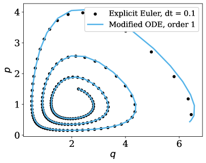
(a) $h=0.1,T=10$

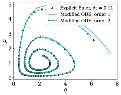
(b) $h=0.11,T=10$

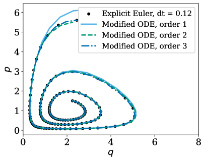
(c) $h=0.12,T=10$

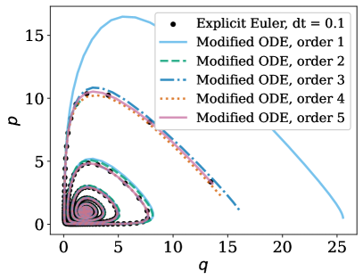
(d) $h=0.1$, $T=66.4$

Figure 1. Numerical solutions of the Lotka-Volterra system with final time $T$ by the explicit Euler method with fixed time step size $h$ and reference solutions of corresponding modified equations.

2.5. Modifying integrators

In the previous section we saw that we could accurately determine the behavior of the explicit Euler method for the Lotka-Volterra system by deriving increasingly accurate modified equations. Nevertheless, the method’s qualitative behavior remains completely different from that of the true solution (which, for the prescribed conditions, is periodic). In this section, we instead seek to modify the right-hand-side $f(y)$ to obtain a perturbation $f_{h}(y)$ so that when the explicit Euler method is applied to $f_{h}(y)$ it yields a solution that matches the exact solution of the original problem $f(y)$. This approach is referred to as a modifying integrator; i.e. the integrator modifies the ODE.

In terms of B-series, we want to obtain the exact solution B-series when we substitute the modified RHS into our numerical method:

$$B(u,B(v,hf,\cdot),y)=B(e,hf,y)$$

Here $B(u,hf,y)$ is the B-series of our numerical method (in this case, explicit Euler) while $B(v,hf,y)$ is the B-series of the modified equation. We see that we have $(v\star u)(\tau)=e(\tau)$.

Results for the case at hand are shown in Figure 2. The left figure shows the exact solution and the numerical solution of the original problem, while the right figure shows solutions of the modifying integrator systems of orders 1, 2, and 3. We see that the first-order modifying integrator system still exhibits growth, though it is greatly reduced compared to the Euler solution of the original system. The second-order modifying integrator is actually dissipative. The third-order modifying integrator is indistinguishable from the exact solution at this scale and is nearly periodic.

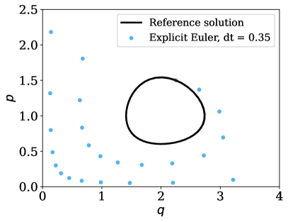
(a) Exact solution and explicit Euler solution.

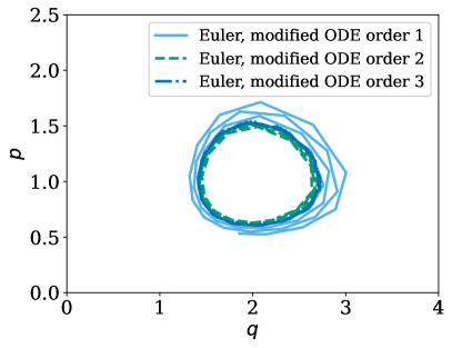
(b) Solutions of modifying integrators of orders 1-3.

Figure 2. Numerical solutions of the modifying integrator system corresponding to the Lotka-Volterra equations and explicit Euler method.

2.6. A special RK method and ODE pair

In this section we study the application of the explicit midpoint Runge-Kutta method

(64a) $$Y_{2} =y_{n}+\frac{h}{2}f(y_{n}),$$

(64b) $$y_{n+1} =y_{n}+hf(Y_{2}),$$

applied to the nonlinear oscillator problem

(65a) $$\dot{p}(t) =\frac{-q}{p^{2}+q^{2}},$$

(65b) $$\dot{q}(t) =\frac{p}{p^{2}+q^{2}}.$$

Solutions of (65) are periodic, forming circles in the $p-q$ plane, but with period depending on the initial energy $\beta^{2}=\|y(0)\|^{2}$, which is conserved:

(66) $$y(t) =\beta\begin{bmatrix}\cos(t/\beta^{2})\\ \sin(t/\beta^{2})\end{bmatrix}.$$

The numerical solution obtained by application of (64) to (65) turns out to be

(67) $$y_{n}=\beta\begin{bmatrix}\cos(n\theta(h/\beta^{2}))\\ \sin(n\theta(h/\beta^{2}))\end{bmatrix},\quad\text{where }\theta(\mu)=\arccos\left(\frac{1-\frac{\mu^{2}}{4}}{1+\frac{\mu^{2}}{4}}\right).$$

This can be verified by substituting (67) into (64) and solving for $\theta$, noting that the given value solves both of the resulting equations. As studied in (Ranocha and Ketcheson, 2020, Section 5.1), the midpoint method (64) has the remarkable property that it conserves the energy exactly for (65) for any step size. As far as we are aware, this behavior is unique among explicit discretizations of initial value ODEs. The backward error analysis of this example was our initial motivation for developing BSeries.jl.

2.6.1. Modified equation analysis

The modified equation (up to order eight) for this example can be obtained with the following code:

    using BSeries, StaticArrays, SymPy

    A = @SArray [0 0; 1//2 0]
    b = @SArray [0, 1//1]
    c = @SArray [0, 1//2]

    u = symbols("p,q")
    h = symbols("h")
    f = [-u[2], u[1]] / (u[1]^2 + u[2]^2)

    modified_equation(f, u, h, A, b, c, 8);

After some cleaning up, we find that the modified equation RHS is closely related to the original RHS:

(68) $$f_{h}(y)=f(y)g(h/\|y\|^{2})$$

where $g$ is a function of one variable, with the first terms in its power series (obtained from the code above) being

(69) $$g(z)=1-\frac{z^{2}}{12}+\frac{z^{4}}{80}-\frac{z^{6}}{448}+\frac{z^{8}}{2304}+{\mathcal{O}}(z^{10}).$$

In fact, this structure could be anticipated because the Hamiltonian structure of (65) implies that the even-order derivatives of $f$ are proportional to $f$, while odd-order derivatives are proportional to $y$. This means that any odd-order derivative terms would be non-conservative, whereas (since we know the midpoint method is energy-conservative) (Hairer et al., 2013, Corollary IX.5.3) guarantees that every truncation of the modified equation B-series must be conservative.

For this example we can find $f_{h}$ in an alternative and more direct way. From (66) we have

$$y_{h}(h) =\beta\begin{bmatrix}\cos(\theta(h/\beta^{2}))\\ \sin(\theta(h/\beta^{2}))\end{bmatrix}$$

and differentiating both sides with respect to $h$ yields

$$y_{h}^{\prime}(h) =\beta\begin{bmatrix}-\sin(\theta(h/\beta^{2}))\\ \cos(\theta(h/\beta^{2}))\end{bmatrix}\frac{d}{dh}\theta(h/\beta^{2})$$

$$=f(y_{h}(h))\theta^{\prime}(h/\beta^{2}).$$

Comparing with (68), we see that

(70) $$g(z) =\frac{d}{dz}\arccos\left(\frac{1-\frac{z^{2}}{4}}{1+\frac{z^{2}}{4}}\right)=2\arctan(z/2).$$

This also implies that the midpoint method is symmetric (in the sense of (Hairer et al., 2013)) for this problem. This can be verified directly by checking that (66) is the solution obtained with the adjoint of the midpoint method, which is

(71a) $$Y_{1} =y_{n}+hf(Y_{1})-\frac{h}{2}f(Y_{2})$$

(71b) $$y_{n+1}=Y_{2} =y_{n}+hf(Y_{1}).$$

It is important to note that the explicit midpoint method is not symmetric for general ODEs; the B-series for (64) for a general RHS $f$ includes both even- and odd-order derivatives. Thus the behavior observed in this example results from a (seemingly very fortuitous) cancellation of terms at every odd order in $h$. At order $h^{5}$, there are 16 (out of 20) coefficients in the modified equation for (64) that are non-zero, but their sum when multiplied by the elementary differentials corresponding to (65) is zero. The method and the problem appear to possess a complementary structure.

2.6.2. Modifying integrator

We can also construct a modifying integrator for this problem. Again using BSeries.jl we find that, up to terms of order $h^{4}$, we have

$$\hat{f}_{h}(y)=f(y)\hat{g}_{4}(h/\|y\|^{2}),$$

where $f(y)$ is the right hand side of the original problem (65) and

$$\hat{g}_{4}(z):=1+\frac{z^{2}}{12}+\frac{z^{4}}{20}.$$

We see that the right hand side is again Hamiltonian at each order, and we might conjecture that $\hat{f}_{h}$ will have this structure at every order. However, continuing the calculation up to terms of order $h^{7}$ yields

(72) $$\hat{f}_{h}(y)=f(y)\hat{g}_{6}(h/\|y\|^{2})+y\left(\frac{h^{5}}{48\|y\|^{12}}+\frac{31h^{7}}{640\|y\|^{16}}\right)$$

where

$$\hat{g}_{6}(z):=\hat{g}_{4}(z)+\frac{127}{2016}z^{6}.$$

We see that the truncations of the modifying integrator system are not Hamiltonian (for order $h^{5}$ and higher).

The energy and error of numerical solutions of the explicit midpoint method (64) applied to the nonlinear oscillator (65) and the corresponding modifying integrator equation (72) for two choices of the constant time step size $h$ are shown in Figure 2.6.2. Initially, the modifying integrator approach yields a much more accurate solution (since it results in an eighth-order approximation instead of a second-order one). However, the error growth rate in time is larger since the energy is not conserved. Thus, the energy-conserving explicit midpoint method can have a smaller error for large times. However, this asymptotic regime depends on the chosen time step size. If $h$ is small enough, the increased order of accuracy of the modifying integrator approach makes it advantageous until both methods yield approximately 100% error.

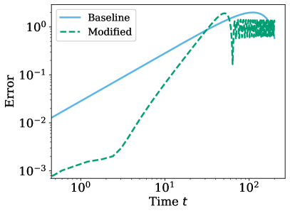
(a) Error, $h=0.6$

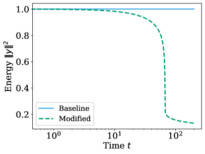
(b) Energy, $h=0.6$

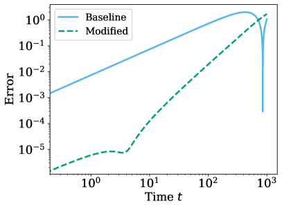
(c) Error, $h=0.3$

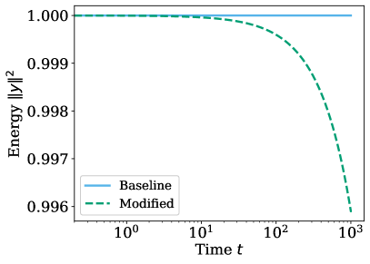
(d) Energy, $h=0.3$

Figure 3. Error and energy of numerical solutions of the explicit midpoint method (64) with fixed time step size $h$ for the nonlinear oscillator (65) and the corresponding modifying integrator equation (including terms of order $h^{7}$).

3. B-series for other classes of methods

The historical development of B-series is closely intertwined with that of Runge-Kutta methods, and Runge-Kutta methods (and their generalizations) continue to be the primary area of application for B-series. Nevertheless, B-series are also used in the analysis of other classes of methods, and BSeries.jl can be used for this purpose. In Section 3.1 we discuss application to additive Runge-Kutta methods. In Section 3.2 we present the construction and analysis of the B-series and modified equation of the average vector field (AVF) method (McLachlan et al., 1999).

3.1. Additive Runge-Kutta methods

Many time integration methods outside the class of Runge-Kutta methods – such as partitioned RK methods (Hairer et al., 2013, Section III.2) and Runge-Kutta-Nyström methods (Hairer et al., 1993, Section II.14) – can be represented using generalizations of B-series based on colored rooted trees. Colored rooted trees are also called $N$-trees (Araújo et al., 1997) or $P$-trees (Hairer, 1981). The corresponding generalized B-series are also called NB-series (Araújo et al., 1997) or P-series (Hairer, 1981), depending on the context. Here, we briefly discuss the extension of B-series to additive Runge-Kutta (ARK) methods (a superset of partitioned RK methods) and functions on trees to colored rooted trees, following (Araújo et al., 1997).

For an additive ODE

(73) $$\dot{y}(t)=\sum_{\nu=1}^{N}f^{\nu}\bigl{(}y(t)\bigr{)}$$

with $N\in\mathbb{N}$, an additive Runge-Kutta method performs a step from $y_{n}$ to $y_{n+1}$ via

(74a) $$Y_{i} =y_{n}+h\sum_{\nu=1}^{N}\sum_{j=1}^{s}a_{ij}^{\nu}f^{\nu}(Y_{j}),$$

(74b) $$y_{n+1} =y_{n}+h\sum_{\nu=1}^{N}\sum_{j=1}^{s}b_{j}^{\nu}f^{\nu}(Y_{j}).$$

The Butcher coefficients are $A^{\nu}=(a_{ij}^{\nu})_{i,j=1}^{s}$, $b^{\nu}=(b_{j}^{\nu})_{j=1}^{s}$, $\nu\in\{1,\dots,N\}$. Here, we assumed again an autonomous form of the ODE. The same analysis applies to ARK methods satisfying the row-sum condition.

We study an example of an additive ODE and ARK method in Section 3.1.2. But first we briefly discuss the extension of the theory of rooted trees and B-series to such objects.

3.1.1. Colored rooted trees

The solution map corresponding to an ARK method can be represented by an infinite sum whose terms are in one-to-one correspondence with colored rooted trees. Each node in a colored rooted tree has an associated color, which can also be represented by an integer $\nu\in\{1,2,\dots,N\}$ corresponding to a term $f^{\nu}$ in (73). Each tree has an associated elementary differential, which is identical to that of the corresponding uncolored tree except that each factor involving a derivative of $f$ now involves the corresponding $f^{\nu}$. For example, let $N=2$ and (for clarity) write $f^{1}=f$, $f^{2}=g$. Some examples of elementary differentials are as follows:

$$F\left(\Forest{bigrootedtree[[[.,graynode]]]}\right) =f^{j}_{k}f^{k}_{l}g^{l} F\left(\Forest{bigrootedtree[.,graynode[[][.,graynode]]]}\right) =g^{j}_{k}f^{k}_{lm}f^{l}g^{m}.$$

In a similar way, the elementary weight of a colored rooted tree is identical to that of the uncolored tree except that the coefficients $A,b$ associated with each node are replaced by $A^{\nu},b^{\nu}$ where $\nu$ is the color of the node. Some examples of elementary weights for bicolored trees are as follows:

$$\Phi\left(\Forest{bigrootedtree[[[.,graynode]]]}\right) =\sum_{j,k,l}b^{1}_{j}a^{1}_{jk}a^{2}_{kl} \Phi\left(\Forest{bigrootedtree[.,graynode[[][.,graynode]]]}\right) =\sum_{j,k,l,m}b^{2}_{j}a^{1}_{jk}a^{1}_{kl}a^{2}_{km}.$$

In the code, we represent colored rooted trees using a color sequence in addition to the level sequence. The algorithms such as the generation of the partitions are extended correspondingly. The generation of all colored rooted trees extends the algorithm of (Beyer and Hedetniemi, 1980) by iterating over all level sequences at the outer level and all color sequences in an inner iteration; this inner iteration needs to ensure that the color sequence yields a canonical representation, which is extended to colored rooted trees by additional lexicographic comparison of the color sequences after the usual lexicographic comparison of the level sequences.

3.1.2. Störmer-Verlet method as additive Runge-Kutta method

Consider the Kepler problem

(75) $$\dot{q}(t)=p,\quad\dot{p}(t)=g(q)=\frac{q}{|q|^{3}},$$

with momentum $p=(p_{1},p_{2})$ and position $q=(q_{1},q_{2})$. This is an example of an additive ODE (73) with $N=2$ and

(76) $$f^{1}(q,p)=\begin{pmatrix}p\\ 0\end{pmatrix},\quad f^{2}(q,p)=\begin{pmatrix}0\\ q/|q|^{3}\end{pmatrix}.$$

The classical Störmer-Verlet method

(77) $$p_{n+1/2} =p_{n}+\frac{h}{2}g(q_{n}),$$

$$q_{n+1} =q_{n}+hp_{n+1/2},$$

$$p_{n+1} =p_{n+1/2}+\frac{h}{2}g(q_{n+1}),$$

can be interpreted as an ARK method (74) with $N=2$ and coefficients

(78) $$A^{1}=\begin{pmatrix}0&0\\ 1/2&1/2\end{pmatrix},b^{1}=\begin{pmatrix}1/2\\ 1/2\end{pmatrix},\quad A^{2}=\begin{pmatrix}1/2&0\\ 1/2&0\end{pmatrix},b^{2}=\begin{pmatrix}1/2\\ 1/2\end{pmatrix},$$

cf. Table II.2.1 of (Hairer et al., 2013). Although these coefficients look like those of an implicit method, they result in the explicit Störmer-Verlet method since $f^{1}(q,p)$ influences only $q$ and does not depend on $q$ while $f^{2}(q,p)$ influences only $p$ and does not depend on $p$.

Computing the modified equation up to terms of order $h^{7}$ using BSeries.jl reveals that there are no terms proportional to odd powers of $h$, in accordance with the well-known symplectic property of the method.

Next we consider improving the accuracy of the Störmer-Verlet method for Kepler’s problem by applying the modifying integrator approach, using BSeries.jl, up to order four. The resulting modifying integrator equations include the following equation for $q_{1}$:

(79) $$\dot{q}_{1}(t)=p_{1}+\frac{h^{2}}{6}\left(p_{1}\left(\frac{3q_{1}^{2}}{\left(q_{1}^{2}+q_{2}^{2}\right)^{\frac{5}{2}}}-\frac{1}{\left(q_{1}^{2}+q_{2}^{2}\right)^{\frac{3}{2}}}\right)+\frac{3p_{2}q_{1}q_{2}}{\left(q_{1}^{2}+q_{2}^{2}\right)^{\frac{5}{2}}}\right).$$

We see that there are no third-order terms (as expected for this symmetric method). However, since $q$ appears on the right hand side, the method is no longer explicit. We conclude that this does not appear to be an appealing approach. The code for this example is accessible in our reproducibility repository (Ketcheson and Ranocha, 2021).

3.2. The average vector field method

The AVF method takes the form

(80) $$y_{n+1}=y_{n}+h\int_{0}^{1}f\bigl{(}\xi y_{n+1}+(1-\xi)y_{n}\bigr{)}\mathrm{d}\xi.$$

It is a B-series method, with coefficients given explicitly as

(81) $$b(\Forest{rootedtree[]}) =1,$$

(82) $$b([t_{1},...,t_{n}]) =b(t_{1})...b(t_{n})/(n+1);$$

see (Quispel and McLaren, 2008; Celledoni et al., 2009). We can instantiate this method in BSeries.jl with the following code:

using BSeries

series = bseries(5) do t, series
    if order(t) in (0, 1)
        return 1 // 1
    else
        v = 1 // 1
        n = 0
        for subtree in SubtreeIterator(t)
            v *= series[subtree]
            n += 1
        end
        return v / (n + 1)
    end
end

Here we have generated the B-series up to order five. The energy-preserving property of the method can be checked by considering its modified equation (Celledoni et al., 2010), which we do as follows:

meq = modified_equation(series)
println(latexify(meq, reduce_order_by=1, cdot=false))

which yields the modified equation with

$$f_{h}=F_{f}\mathopen{}\left(\Forest{rootedtree[]}\right)\mathclose{}+\frac{1}{12}h^{2}F_{f}\mathopen{}\left(\Forest{rootedtree[[[]]]}\right)\mathclose{}+\frac{1}{80}h^{4}F_{f}\mathopen{}\left(\Forest{rootedtree[[[[[]]]]]}\right)\mathclose{}+\frac{1}{180}h^{4}F_{f}\mathopen{}\left(\Forest{rootedtree[[[[][]]]]}\right)\mathclose{}+\frac{1}{360}h^{4}F_{f}\mathopen{}\left(\Forest{rootedtree[[[[]][]]]}\right)\mathclose{}+\frac{-1}{180}h^{4}F_{f}\mathopen{}\left(\Forest{rootedtree[[[[]]][]]}\right)\mathclose{}$$

$$+\frac{-1}{720}h^{4}F_{f}\mathopen{}\left(\Forest{rootedtree[[[][][]]]}\right)\mathclose{}+\frac{-1}{180}h^{4}F_{f}\mathopen{}\left(\Forest{rootedtree[[[][]][]]}\right)\mathclose{}+\frac{1}{360}h^{4}F_{f}\mathopen{}\left(\Forest{rootedtree[[[]][[]]]}\right)\mathclose{}+\frac{-1}{720}h^{4}F_{f}\mathopen{}\left(\Forest{rootedtree[[[]][][]]}\right)\mathclose{}.$$

This reproduces the formula given at the top of p. 679 of (Celledoni et al., 2010), demonstrating the energy-preserving property (at least up to the order $h^{4}$ terms). It is straightforward to study higher-order terms in the same way.

4. Implementation and performance

We have developed BSeries.jl and RootedTrees.jl together to get reasonably efficient libraries that allow working with high-order representations of B-series. Of course, the increasing number of elementary differentials of a given order makes explicit calculations infeasible beyond some order. We tried to make this order as high as reasonably possible without increasing the code complexity too much. In this section we explain some of the design choices and optimizations that have been made. Additional performance optimizations that could be implemented in the future include parallel computation and memoization, which which could increase the runtime efficiency of some parts at the cost of a higher memory footprint and/or higher code complexity.

Before discussing some of the design decisions of BSeries.jl related to computational performance, we compare its efficiency to pybs (Sundklakk, 2015). Since pybs uses lazy representations of B-series up to an arbitrary order, we need to instantiate the coefficients for a reasonable comparison. Here, we set up the B-series of the explicit midpoint method with Butcher tableau

(86) $$\begin{array}[]{c|cc}0&0&\\ \frac{1}{2}&\frac{1}{2}&0\\[2.84544pt] \hline\cr&0&1\end{array}$$

and sum the coefficients of the B-series of its modified equation up to order nine. On an Intel® Core™ i7-8700K from 2017, this takes approximately $53\text{\,}\mathrm{ms}$ with BSeries.jl and $3.7\text{\,}\mathrm{s}$ with pybs. Thus, BSeries.jl is approximately 70x faster than pybs for this calculation. All source code and instructions required to reproduce these results are available in our reproducibility repository (Ketcheson and Ranocha, 2021).

The first design decision of BSeries.jl is the choice of programming language. We chose Julia (Bezanson et al., 2017) since it provides convenient high-level abstractions, interactive workflows, and efficient computations enabled via compilation to native machine code. In fact, Julia can be at least as fast as low-level code written in traditional programming languages such as Fortran, C, and C++ (Elrod, 2021; Ranocha et al., 2022).

4.1. Representation of rooted trees

Many performance-related design decisions of BSeries.jl are based on the representation of rooted trees. Since RootedTrees.jl uses canonical level sequences stored in arrays for this purpose, we adopted the same convention when extending it with the functionality required for BSeries.jl.

This convention is convenient when iterating over all rooted trees of a given order since we can use the algorithm of (Beyer and Hedetniemi, 1980) directly. Moreover, this representation is memory efficient with good data locality. Additionally, it simplifies the computation of certain functions on rooted trees such as its symmetry $\sigma$ since identical subtrees are always adjacent to each other.

On the other hand, implementing the composition $\cdot$ or the substitution $\star$ using level sequences requires frequent memory movement. Moreover, the assumption of a canonical representation requires that we sort level sequences of newly created rooted trees, e.g., trees of the partition forest or the partition skeleton.

An alternative representation of rooted trees is based on linked lists of their vertices. The advantages and disadvantages of such a representation and array-based level sequences are basically mirrors of each other. We did not perform extensive benchmarks of both possibilities. Instead, we implemented workarounds for most common performance pitfalls of array-based level sequences. For example, we keep track of some internal buffers in RootedTrees.jl that allow us to avoid dynamic memory allocations when sorting level sequences to obtain canonical representations. Some other performance optimizations are described below.

4.2. Composition and substitution laws

In the literature there exist different algorithmic approaches to the composition and substitution laws, all in terms of rooted trees. In our implementation we have followed the work of Chartier et al. (Chartier et al., 2010). Computing the coefficients of the composition of two B-series requires iterating over all splittings of each tree. Similarly, the substitution law requires iterating over all partitions of a rooted tree. Individually, each of these operations requires iterating over the splitting forest or partition forest of a tree. To reduce the pressure on memory and keep data locality, we use lazy iterators for these tasks. Similarly, we also use lazy iterators when iterating over all rooted trees of a given order.

High-level pseudocode for finding all partitions of a tree (the key to the substitution law) is given in Algorithms 1–3, in order to illustrate some of the performance considerations. These algorithms use lists storing the partition forests/skeletons for clarity and simplicity or presentation; the efficient implementations used for the substitution law use lazy iterators instead. We iterate over binary sequences where each 1 corresponds to an edge that is kept (solid edges in Table 2) and each 0 corresponds to an edge that is removed (dashed edges in Table 2). When executing the while-loops in Algorithms 2 and 3, in which subtrees are removed from the initial tree, we work backwards from the end of the level sequence. Compared to beginning at the root, this reduces the amount of memory moves on average since some nodes have already been removed. Additionally, we use views into existing memory instead of copying parts of level sequences to new arrays whenever possible.

Algorithm 1 Find all partition forests and corresponding skeletons of a tree $\tau$

$m\leftarrow|\tau|$

forests $\leftarrow$ [] $\triangleright$ Empty list

partitions $\leftarrow$ []

for  edge_set in (all binary sequences of length $m$) do $\triangleright$ Edges marked zero are removed

     Append partition_forest($\tau$, edge_set) to forests

     Append skeleton($\tau$, edge_set) to skeletons

end for

procedure partition_forest($\tau$, edge_set)

     forest $\leftarrow$ [] $\triangleright$ Empty list

     while 0 in edge_set do

         $i\leftarrow$ index of next edge marked 0

         remove from $\tau$ edge $i$ and its descendants

         append the removed subtree to forest

         delete entry $i$ from edge_set

     end while

     append $\tau$ to forest

     return forest

end procedure

Algorithm 2 Find the partition forest corresponding to a tree $\tau$ and subset of its edges

procedure skeleton($\tau$, edge_set)

     while 1 in edge_set do

         $i\leftarrow$ index of next edge marked 1

         Contract edge $i$ of $\tau$ by removing the child node and promoting its descendants

         delete entry $i$ from edge_set

     end while

     return $\tau$

end procedure

Algorithm 3 Find the skeleton corresponding to a tree $\tau$ and subset of its edges

The computation of modifying integrators benefits from additional checks in the composition law: If the coefficient of the partition skeleton is zero, there is no need to iterate over the associated partition forest, see (50). This is particularly useful when computing the modified integrator since we need to substitute the modifying integrator series into the B-series of the numerical integrator. By construction, many coefficients of the B-series of explicit Runge-Kutta methods are zero since they involve powers of the strictly lower diagonal matrix $A$. For example, computing the coefficients of the modifying integrator of the explicit midpoint method up to order nine takes approximately $23\text{\,}\mathrm{ms}$ while the same task for the modified equation takes approximately $52\text{\,}\mathrm{ms}$.

4.3. Symbolic calculations

Multiple symbolic computation packages are available in Julia, each with certain strengths and weaknesses. Therefore, we use Julia’s efficient dispatch mechanism to support different symbolic packages (SymPy.jl, Symbolics.jl, and SymEngine.jl) as backends in BSeries.jl. This allows users to choose a package based on their needs. At the time of writing, we often use SymPy.jl for calculations that should be rendered directly in LaTeX, Symbolics.jl when we want to create efficient Julia functions from symbolic computations, and SymEngine.jl when performance matters most and we are mostly interested in symbolic expressions after inserting specific initial values.

To compare the relative performance of different symbolic backends, we measured the time to compute the B-series of the modifying integrator of the explicit midpoint method (64) specialized to the nonlinear oscillator (65) up to order eight and to substitute the initial condition $(0,1)$ into the resulting symbolic expressions. Using current versions of all packages at the time of writing, SymEngine.jl is several orders of magnitude faster than the other two alternatives; see Table 4.

Table 4. Micro-benchmarks of different symbolic backends supported by BSeries.jl for computing the B-series of the explicit midpoint method specialized to the nonlinear oscillator discussed in Section 2.6. Note the different units of time (seconds and milliseconds).

	Computing the B-series	Substituting the initial condition
SymPy.jl	$(1.811\pm 20.118)\text{\times}{10}^{-3}\text{\,}\mathrm{s}$	$212.317\pm 9.885\text{\,}\mathrm{ms}$
Symbolics.jl	$710.232\pm 21.727\text{\,}\mathrm{ms}$	$(2.565\pm 2.848)\text{\times}{10}^{-3}\text{\,}\mathrm{s}$
SymEngine.jl	$15.768\pm 7.733\text{\,}\mathrm{ms}$	$3.353\pm 0.271\text{\,}\mathrm{ms}$

The performance optimizations for symbolic computations in BSeries.jl are orthogonal to the choice of specific backend. They are mostly related to programming approaches and the use of information available from analytical theorems. For example, we use a dynamic programming approach to determine elementary differentials of symbolic functions, i.e., we compute all elementary differentials up to a specified order upfront, allowing us to re-use lower order differentials when computing higher order ones. In addition, we use Schwarz’s theorem to reduce the number of symbolic differentiation steps by making use of symmetry properties of higher-order derivatives.

5. Conclusion

B-series are fascinating objects that lie at the intersection of continuous and discrete, as well as pure and applied, mathematics. The package BSeries.jl makes it straightforward to apply B-series analysis to any Runge-Kutta method and/or initial value ODE. Most applications of B-series in the literature are limited to lower order in $h$ due to the combinatorial explosion of terms that must be dealt with; BSeries.jl makes it possible to work effectively and efficiently with series up to much higher order in $h$, thus automating backward error analysis for discretizations of nonlinear ODE systems. We hope that BSeries.jl will also enable continued advances in our understanding of numerical integrators. Furthermore, since renormalization in quantum field theory is known also to rely on the Hopf algebra structure implemented in BSeries.jl (Connes and Kreimer, 2000), this package may be useful for calculations in that domain.

There are many potential areas for future extension of BSeries.jl, corresponding to the wide range of applications of B-series; these include B-series for partitioned methods, multistep methods, multiderivative methods, exponential methods, and Rosenbrock methods.

References

- (1)
- Araújo et al. (1997) AL Araújo, Ander Murua, and Jesús María Sanz-Serna. 1997. Symplectic methods based on decompositions. SIAM J. Numer. Anal. 34, 5 (1997), 1926–1947. https://doi.org/10.1137/S0036142995292128
- Beyer and Hedetniemi (1980) Terry Beyer and Sandra Mitchell Hedetniemi. 1980. Constant time generation of rooted trees. SIAM J. Comput. 9, 4 (1980), 706–712. https://doi.org/10.1137/0209055
- Bezanson et al. (2017) Jeff Bezanson, Alan Edelman, Stefan Karpinski, and Viral B Shah. 2017. Julia: A Fresh Approach to Numerical Computing. SIAM Rev. 59, 1 (2017), 65–98. https://doi.org/10.1137/141000671 arXiv:1411.1607
- Bornemann (2001) Folkmar Bornemann. 2001. Runge-Kutta methods, trees, and Maple. Selçuk Journal of Applied Mathematics 2 (2001), 3–15.
- Bornemann (2002) Folkmar Bornemann. 2002. Runge-Kutta methods, trees, and Mathematica. arXiv:math/0211049
- Butcher (2009) JC Butcher. 2009. B-series and B-series Coefficients. In AIP Conference Proceedings, Vol. 1168. American Institute of Physics, 7–10.
- Butcher (1969) J. C. Butcher. 1969. The effective order of Runge-Kutta methods. In Conference on the Numerical Solution of Differential Equations, J. Li. Morris (Ed.). Springer Berlin Heidelberg, Berlin, Heidelberg, 133–139.
- Butcher (1972) John C Butcher. 1972. An algebraic theory of integration methods. Math. Comp. 26, 117 (1972), 79–106.
- Butcher (2008) J. C. Butcher. 2008. Numerical Methods for Ordinary Differential Equations (2 ed.). Wiley.
- Butcher (2021) John Charles Butcher. 2021. B-series: algebraic analysis of numerical methods. Vol. 55. Springer Nature.
- Cameron (2006) Frank Cameron. 2006. A Matlab package for automatically generating Runge-Kutta trees, order conditions, and truncation error coefficients. ACM Transactions on Mathematical Software (TOMS) 32, 2 (2006), 274–298.
- Celledoni et al. (2009) Elena Celledoni, Robert I McLachlan, David I McLaren, Brynjulf Owren, G Reinout W Quispel, and William M Wright. 2009. Energy-preserving Runge-Kutta methods. ESAIM: Mathematical Modelling and Numerical Analysis 43, 4 (2009), 645–649.
- Celledoni et al. (2010) Elena Celledoni, Robert I McLachlan, Brynjulf Owren, and GRW Quispel. 2010. Energy-preserving integrators and the structure of B-series. Foundations of Computational Mathematics 10, 6 (2010), 673–693.
- Chartier et al. (2010) Philippe Chartier, Ernst Hairer, and Gilles Vilmart. 2010. Algebraic Structures of B-series. Foundations of Computational Mathematics 10, 4 (March 2010), 407–427. https://doi.org/10.1007/s10208-010-9065-1
- Connes and Kreimer (2000) Alain Connes and Dirk Kreimer. 2000. Renormalization in quantum field theory and the Riemann–Hilbert problem I: The Hopf algebra structure of graphs and the main theorem. Communications in Mathematical Physics 210, 1 (2000), 249–273.
- Elrod (2021) Chris Elrod. 2021. Roadmap to Julia BLAS and Linear Algebra. https://www.youtube.com/watch?v=KQ8nvlURX4M. Talk presented at JuliaCon.
- Famelis et al. (2004) I Th Famelis, SN Papakostas, and Ch Tsitouras. 2004. Symbolic derivation of Runge–Kutta order conditions. Journal of Symbolic Computation 37, 3 (2004), 311–327.
- Gowda et al. (2021) Shashi Gowda, Yingbo Ma, Alessandro Cheli, Maja Gwozdz, Viral B Shah, Alan Edelman, and Christopher Rackauckas. 2021. High-performance symbolic-numerics via multiple dispatch. arXiv:2105.03949
- Gruntz (1995) Dominik Gruntz. 1995. Symbolic computation of explicit Runge-Kutta formulas. In Solving Problems in Scientific Computing Using Maple and MATLAB®. Springer, 267–283.
- Hairer (1981) Ernst Hairer. 1981. Order conditions for numerical methods for partitioned ordinary differential equations. Numer. Math. 36, 4 (1981), 431–445. https://doi.org/10.1007/BF01395956
- Hairer et al. (2013) Ernst Hairer, Christian Lubich, and Gerhard Wanner. 2013. Geometric Numerical Integration: Structure-Preserving Algorithms for Ordinary Differential Equations. Vol. 31. Springer Science & Business Media.
- Hairer et al. (1993) Ernst Hairer, Syvert P. Nørsett, and G. Wanner. 1993. Solving ordinary differential equations {I}: Nonstiff Problems (second ed.). Springer, Berlin.
- Hairer and Wanner (1974) Ernst Hairer and Gerhard Wanner. 1974. On the Butcher group and general multi-value methods. Computing 13, 1 (1974), 1–15.
- Karam et al. (2020) Mokbel Karam, James C Sutherland, and Tony Saad. 2020. PyModPDE: A python software for modified equation analysis. SoftwareX 12 (2020), 100541.
- Ketcheson (2021) David I Ketcheson. 2021. BSeries.py. https://github.com/ketch/bseries.
- Ketcheson and Ranocha (2021) David I Ketcheson and Hendrik Ranocha. 2021. Reproducibility repository for Computing with B-series. https://github.com/ketch/bseries-package-notebooks. https://doi.org/10.5281/zenodo.5716612
- Ketcheson et al. (2020) David I Ketcheson, Hendrik Ranocha, Matteo Parsani, Umair bin Waheed, and Yiannis Hadjimichael. 2020. NodePy: A package for the analysis of numerical ODE solvers. (2020).
- Knoth (2021) Oswald Knoth. 2021. BSeries. https://github.com/OsKnoth/B-Series.
- LeVeque (2007) Randall J. LeVeque. 2007. Finite Difference Methods for Ordinary and Partial Differential Equations: steady-state and time-dependent problems. SIAM.
- McLachlan et al. (1999) Robert I McLachlan, G Reinout W Quispel, and Nicolas Robidoux. 1999. Geometric integration using discrete gradients. Philosophical Transactions of the Royal Society of London. Series A: Mathematical, Physical and Engineering Sciences 357, 1754 (1999), 1021–1045.
- Meurer et al. (2017) Aaron Meurer, Christopher P. Smith, Mateusz Paprocki, Ondřej Čertík, Sergey B. Kirpichev, Matthew Rocklin, AMiT Kumar, Sergiu Ivanov, Jason K. Moore, Sartaj Singh, Thilina Rathnayake, Sean Vig, Brian E. Granger, Richard P. Muller, Francesco Bonazzi, Harsh Gupta, Shivam Vats, Fredrik Johansson, Fabian Pedregosa, Matthew J. Curry, Andy R. Terrel, Štěpán Roučka, Ashutosh Saboo, Isuru Fernando, Sumith Kulal, Robert Cimrman, and Anthony Scopatz. 2017. SymPy: symbolic computing in Python. PeerJ Computer Science 3 (01 2017), e103. https://doi.org/10.7717/peerj-cs.103
- Quispel and McLaren (2008) GRW Quispel and David Ian McLaren. 2008. A new class of energy-preserving numerical integration methods. Journal of Physics A: Mathematical and Theoretical 41, 4 (2008), 045206.
- Ranocha and contributors (2019) Hendrik Ranocha and contributors. 2019. RootedTrees.jl: A collection of functionality around rooted trees to generate order conditions for Runge-Kutta methods in Julia for differential equations and scientific machine learning (SciML). https://github.com/SciML/RootedTrees.jl. https://doi.org/10.5281/zenodo.5534590
- Ranocha and Ketcheson (2020) Hendrik Ranocha and David I Ketcheson. 2020. Energy Stability of Explicit Runge-Kutta Methods for Non-autonomous or Nonlinear Problems. SIAM Journal On Numerical Analysis 58, 6 (2020), 3382–3405. https://doi.org/10.1137/19M1290346 arXiv:1909.13215
- Ranocha and Ketcheson (2021) Hendrik Ranocha and David I Ketcheson. 2021. BSeries.jl: Computing with B-series in Julia. https://github.com/ranocha/BSeries.jl. https://doi.org/10.5281/zenodo.5534602
- Ranocha et al. (2022) Hendrik Ranocha, Michael Schlottke-Lakemper, Andrew Ross Winters, Erik Faulhaber, Jesse Chan, and Gregor J Gassner. 2022. Adaptive numerical simulations with Trixi.jl: A case study of Julia for scientific computing. Proceedings of the JuliaCon Conferences 1, 1 (01 2022), 77. https://doi.org/10.21105/jcon.00077 arXiv:2108.06476 [cs.MS]
- Sofroniou (1994) Mark Sofroniou. 1994. Symbolic derivation of Runge-Kutta methods. Journal of symbolic computation 18, 3 (1994), 265–296.
- Sundklakk (2015) Henrik Sperre Sundklakk. 2015. A Library for Computing with Trees and B-Series. Master’s thesis. Norwegian University of Science and Technology. http://hdl.handle.net/11250/2352711 Software available at https://github.com/henriksu/pybs.