RIO: Rotation-equivariance supervised learning of robust inertial odometry

Abstract

This paper introduces rotation-equivariance as a self-supervisor to train inertial odometry models. We demonstrate that the self-supervised scheme provides a powerful supervisory signal at training phase as well as at inference stage. It reduces the reliance on massive amounts of labeled data for training a robust model and makes it possible to update the model using various unlabeled data. Further, we propose adaptive Test-Time Training (TTT) based on uncertainty estimations in order to enhance the generalizability of the inertial odometry to various unseen data. We show in experiments that the Rotation-equivariance-supervised Inertial Odometry (RIO) trained with 30% data achieves on par performance with a model trained with the whole database. Adaptive TTT improves models performance in all cases and makes more than 25% improvements under several scenarios.

1 Introduction

Accurate and robust localization with low-cost Inertial Measurement Units (IMUs) is an ideal solution to a wide range of applications from augmented reality[32] to indoor positioning services[28, 33]. An IMU usually consists of accelerometers and gyroscopes, sometimes magnetometers and can sample linear acceleration, angular velocity and magnetic flux density in an energy-efficient way. It can be light-weight and pretty cheap that many mobile devices like smartphones and VR headsets are instrumented with it. In many scenarios such as indoor or underground where global navigation satellite system is not available, ubiquitous IMU is a promising signal source, which can provide reliable and continuous location service. Unlike Visual-Inertial Odometry (VIO)[8] that is sensitive to surroundings and cannot work under extreme lighting, IMU-only inertial odometry is more desired and possible to perform accurate and robust localization every time and everywhere[10, 18].

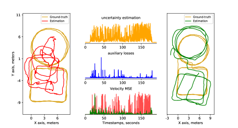
Figure 1: An example trajectory estimation improved by RIO. On the left, we show original model performance before rotation-equivariance supervised learning and right is the result of RIO. In the middle, we show uncertainty estimation (orange), auxiliary losses (blue) computed by the self-supervised task, original estimated velocity MSE (red) and updated model velocity MSE (green).

Recent advances of data-driven approaches (e.g., IONet[4], RoNIN[12], TLIO[18]) based on machine learning and deep learning have pushed the limit of traditional inertial odometry[20, 13] with the help of kinematic model and prior knowledge. However, to the best of our knowledge, all of them are based on purely supervised learning, which is notoriously weak under distribution shifts. IMU sensor data varies widely with different devices and users, sometimes the sensor data drifts over time. It is hard to control the distribution variability when the supervised algorithms are deployed in diverse applications. A rich and diverse database such as RoNIN[12] database can alleviate the problem to some extent, but it is cumbersome to collect such a big database and there are always scenarios that the database does not include and therefore the supervised model cannot capture their characteristics.

In order to mitigate the challenge of distribution shift in real-world, we propose a geometric constraint, rotation-equivariance, that can improve generalizability of deep model in training phase and help the deep model to learn from shifted sensor data at inference time. Inspire by the Heading-Agnostic Coordinate Frame (HACF) presented in RoNIN[12], we define rotation-equivariance that when the IMU sequence in HACF is rotated around Z axis by a random angle, the corresponding ground-truth trajectory should be transformed by the same horizontal rotation. Under this assumption, we propose an auxiliary task that minimizing angle error between deep model prediction for rotated IMU data and rotated prediction of the original data. In experiments we validate that the auxiliary task improves model robustness in training phase when it is jointly optimized with the supervised velocity loss. During inference time, we formulate the auxiliary task as a self-supervised learning problem alone, that we update model parameters based on auxiliary losses generated by test samples to adapt the model to the distribution of given test data. This process is named as Test-Time Training (TTT)[25]. Empirical results of TTT indicate the proposed self-supervision task brings substantial improvements at inference time. Furthermore, we introduce deep ensembles, a promising approach for simple and scalable predictive uncertainty estimation[17]. We show in experiments that the estimated uncertainty using deep ensembles is consistent with the error distribution. It helps us to develop adaptive TTT, that model parameters are updated when the uncertainty of prediction reaches a certain level. We compare different TTT strategies and study the relationship between update frequency and model precision.

In summary, our paper has the following three main contributions:

1. We propose Rotation-equivariance-supervised Inertial Odometry (RIO) and demonstrate that rotation-equivariance can be formulated as an auxiliary task with powerful supervisory signal in training phase.

2. We employ TTT based on rotation-equivariance for learning-based inertial odometry and validate that it helps to improve the generalizability of RIO.

3. We introduce deep ensembles as a practical approach for uncertainty estimation, and utilize the uncertainty result as indicators for adaptively triggering TTT.

The remainder structure of this paper is: we first give an overview on previous work regarding inertial odometry algorithms and related self-supervised tasks. Then we introduce our method and finally present experiments and evaluations.

2 Related work

Roughly, there are three types of inertial odometry algorithms: i) double integration-based analytical solutions[26, 30, 3]; ii) constrained model with additional assumptions[20, 9, 13, 15, 22, 14] and iii) data-driven methods[31, 4, 12, 18, 24, 29].

Conventional strap-down inertial navigation system is to use double integration of IMU readings to compute positions[26]. Many analytical solutions[30, 3] have been studied to promote the performance of the system. However, double integration leads to exploded cumulative error if there are signal biases. It requires high-precision sensors which are expensive and heavy, and typically are instrumented with aircrafts, automobiles and submarines.

For consumer-grade IMUs that are small and cheap but have lower accuracy, a variety of constrained models with different assumptions emerged[15] and mitigated error drifts to some extent. [20, 9] resort to shoe-mounted sensors to detect zero velocity for limiting velocity errors. [13] proposes step-detection and step-length estimation algorithms to estimate walking distance under regular gait hypothesis. Inertial odometry models fused with available measurements by Extended Kalmann Filter (EKF) are presented in [22, 14].[22] requires observations such as position fixes or loop-closures. [14] suppose negligible acceleration of the device equipmented with IMU.

Data-driven methods further broaden applicable scenarios of IMUs and relax condition limitations. RIDI[31] and PDRNet[2] proposes to estimate robust trajectories of natural human motions with supervised training in a hierarchical way. RIDI[31] develop a cascaded regression model that first use a support vector machine to classify IMU placements and then type-specific support vector regression models to estimate velocities. PDRNet[2] employ a smartphone location recognition network to distinguish smartphone locations and then use different models trained for different locations for inference. IONet[4] and RoNIN[12] using unified deep neural networks provide more robust solutions that work in highly dynamic conditions. They show direct integration of estimated velocities helps with limiting error drifts and a unified deep neural network model is capable to generalize to various motions. TLIO[18] introduces a stochastic cloning EKF coupled with the neural network to further reduce position drifts. IDOL[24] and [29] are recent deep learning-based works that release heavy dependent of device orientation. IDOL designs an explicit orientation estimation module relied on magnetometer readings and [29] propose a novel loss formulation to regress velocity from raw inertial measurements.

Our work is in line with data-driven inertial odometry research that focuses on mitigating challenge of distribution shift in real-world. We propose rotation-equivariance as a self-supervision scheme to improve model generalizability and learn from unlabeled data. [5] proposes MotionTransformer framework that uses a shared encoder to transform inertial sequences into a domain-invariant hidden representation with generative adversarial networks. They focus on domain adaptation for long sensory sequences from different domains. Our method mainly deal with distribution shifts over one sensory sequence, and we show obvious improvements with the help of proposed self-supervision task. Notably, our work is a flexible module that can be combined with many other deep learning based approaches like RoNIN, TLIO and IDOL.

Self-supervised tasks provide surrogate supervision signals for representation learning. Learning with self-supervision gains increased interest to improve model performance and avoid intensive manual labeling effort. Many vision tasks utilize self-supervision for pre-training[19] or multitask learning[21]. [34] uses view synthesis as supervisor to learn depth and ego-motion from unstructured video. [1] shows that ego-motion-based supervision learns useful features for multiple vision problems. [16] demonstrates that predicting image rotations is a promising self-supervised task for unsupervised representation learning. [25] uses the image rotation task and creates self-supervised learning problem at test time. They validate their approach with object recognition and show substantial improvements under distribution shifts.

3 RIO

3.1 Rotation-equivariance

Our goal is to develop a self-supervised method to improve the robustness of inertial odometry, and make the model perform well in various scenarios. We observe that the trajectory should be rotated in the same way as the IMU data in HACF when it is rotated around z-axis by a certain angle. We name this property as rotation-equivariance. It provides the benefit to learn a robust inertial odometry.

Specifically, for a sequence of accelerometer data in a world coordinate frame, namely acceleration $A=\{\vec{a}_{t}\}_{t=1}^{n}$ with $\vec{a}_{t}\in\mathbb{R}^{3}$, and gyroscope data for the same period in the same coordinate frame, angular velocity $\Omega=\{\vec{\omega}_{t}\}_{t=1}^{n}$ with $\vec{\omega}_{t}\in\mathbb{R}^{3}$, we randomly select a horizontal rotation $Rot(.|\phi)$ that rotates $A$ and $\Omega$ by $\phi$ degrees around $z$ axis, notate as $A^{\phi}$ and $\Omega^{\phi}$. The neural network model $F(\cdot)$ takes acceleration $A$ and angular velocity $\Omega$ as input and yields a velocity estimation $\vec{v}$ as output:

$$\vec{v}=F(A,\Omega|\theta),$$ (1)

where $\theta$ are learnable parameters of model $F(\cdot)$. With rotation-equivariance, given velocity estimation $\vec{v}_{1}=F(A,\Omega|\theta)$, $\vec{v}_{2}=F(A^{\phi},\Omega^{\phi}|\theta)$, there is only a horizontal rotation $\phi$ between $v_{1}$ and $v_{2}$. That is, if operator $Rot(.|\phi)$ is applied to velocity $v_{1}$ and then get the rotated velocity $v_{1}^{\phi}$, we expect $v_{1}^{\phi}=v_{2}$. Negative cosine similarity [7] is employed to evaluate the difference between the two velocities:

$$\mathcal{D}(v_{1}^{\phi},v_{2})=-\frac{<v_{1}^{\phi},v_{2}>}{\lVert v_{1}^{\phi}\rVert_{2}\cdot\lVert v_{2}\rVert_{2}},$$ (2)

where $<\cdot,\cdot>$ denotes the inner product between vectors. Therefore, we define a self-supervised auxiliary task, that given a set of $N$ training IMU samples $S=\{A_{i},\Omega_{i}\}_{i=1}^{N}$, the neural network model must learn to solve the self-supervised training objective:

$$\min_{\theta}\frac{1}{N}\sum_{i=1}^{N}\mathcal{L}(A_{i},\Omega_{i},\theta),$$ (3)

Where the loss function $\mathcal{L}(A_{i},\Omega_{i},\theta)$ is defined as:

$$\frac{1}{K}\sum_{j=1}^{K}\mathcal{D}(F(A_{i}^{\phi_{j}},\Omega_{i}^{\phi_{j}}|\theta),Rot(F(A_{i},\Omega_{i}|\theta)|\phi).$$ (4)

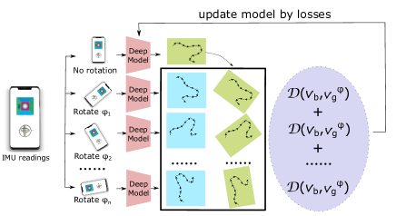
Figure 2: Schematic illustration of proposed RIO. For IMU readings, random angles are selected to generate rotated IMU data. The same deep model is applied to the original and rotated data to estimate trajectories. Estimated trajectory of the original data is rotated by the same set of angles. Estimated trajectories of rotated data are compared with corresponding rotated trajectory estimated by the original data to compute losses and update the deep model.

In the following subsections we describe how the self-supervised auxiliary task helps with model training and inference.

Algorithm 1 Joint-Training

1:for $X,\vec{v}^{gt}$ in loader do $\triangleright$ load a batch with n samples

2:     for each $X_{i},\vec{v}_{i}^{gt}$ do parallel

3:         Random select a angle $\phi_{i}$

4:         $X_{i}^{\phi_{i}}=Rot(X_{i}|\phi_{i})$ $\triangleright$ compute conjugate input

5:         $\vec{v}_{i}=F(X_{i}|\theta)$

6:         $\vec{v}_{i}^{c}=F(X_{i}^{\phi_{i}}|\theta)$ $\triangleright$ compute outputs

7:         $l_{v_{i}}=\sum\limits_{x,y,z}(\vec{v}_{i}-\vec{v}_{i}^{gt})^{2}$ $\triangleright$ compute velocity loss

8:         $\vec{v}_{i}^{\phi_{i}}=Rot(\vec{v}_{i}|\phi_{i})$ $\triangleright$ prepare rotated output

9:         if $\lVert v_{i}\rVert_{2}>0.5$ then

10:              $l_{ssl_{i}}=\mathcal{D}(v_{i}^{\phi_{i}},v_{i}^{c})$ $\triangleright$ compute as Eq. (2)

11:         else

12:              $l_{ssl_{i}}=0$ $\triangleright$ set the loss to zero

13:         end if

14:     end for

15:     $L=\sum\limits_{i}l_{v_{i}}+\sum\limits_{i}l_{ssl_{i}}$

16:     Update $\theta$ using Adam

17:end for

3.2 Joint-Training

In the training phase, we optimize the auxiliary loss (see Eq. (4)) with velocity losses jointly. With the auxiliary task, the neural network model is encouraged to produce velocity estimations with a certain relative geometric relationship. However, it is unrealistic for the model to learn the magnitude and direction of the velocity in a consistent coordinate frame only with the auxiliary task. Jointly, we adopt the robust stride velocity loss to supervise the model. Stride velocity losses compute mean square error between the model output $\vec{v}_{t}$ at time frame $t$ and the ground truth velocity $\vec{v}_{t}^{gt}$ which is calculated by the average velocity over the sensor input time stride. In practice, we take one second sensor data as input and calculate the corresponding average velocity as supervisor.

To train the model on both tasks, we create conjugate data for each training input data and organize them as data pairs. IMU data is sampled at 200 Hz and we take every 200 continuous frames as input. In other words, we use IMU data last for 1 second as input. IMU data and ground truth trajectories are transformed into the same HACF as mentioned in RoNIN[12]. And ground truth velocity is then calculated as the displacement of the corresponding time divide by the time length according to the ground truth trajectory in the HACF. More clearly, at frame $i$, input $X_{i}=(\{\vec{a}_{t}\}_{t=i-199}^{i},\{\vec{\omega}_{t}\}_{t=i-199}^{i})$, and ground truth velocity $\vec{v}^{gt}_{i}=\vec{P}_{i}–\vec{P}_{i-199}$ where $\vec{P}_{i}$ is the position on the trajectory. For each input $X_{i}$, select a random angle $\phi_{i}~{}(0<\phi_{i}\leqslant 2\pi)$ to horizontally rotate accelerations and angular velocities in $X_{i}$ and get the conjugate data $X_{i}^{\phi_{i}}$. $X_{i}$ and its conjugate $X_{i}^{\phi_{i}}$ are processed by the neural network model $F$ and get two outputs as $\vec{v}_{i}=F(X_{i}|\theta)$ and $\vec{v}_{i}^{c}=F(X_{i}^{\phi_{i}}|\theta)$. For output $\vec{v}_{i}$, calculate the stride velocity loss as $(\vec{v}_{i}-\vec{v}_{i}^{gt})^{2}$. As shown in Sec. 3.1, rotate $\vec{v}_{i}$ around z axis by $\phi_{i}$ that $\vec{v}_{i}^{\phi_{i}}=Rot(\vec{v}_{i}|\phi_{i})$ and calculate the negative cosine similarity between $\vec{v}_{i}^{\phi_{i}}$ and $\vec{v}_{i}^{c}$ as the loss for the self-supervised auxiliary task. To avoid ambiguous orientation of the velocity when stationary, we ignore the auxiliary loss when velocity magnitude is no more than $\mathrm{0.5~{}m/s}$. The pseudo-code of joint training can found in Algorithm 1.

3.3 Adaptive TTT

At test time, we propose adaptive TTT based on rotation-equivariance and uncertainty estimation. It helps improve model performance on unseen data which has a large gap with training data. For test samples, we create conjugate data pairs the same as in training phase. With the self-supervised auxiliary task presented in Sec. 3.1, we calculate the auxiliary loss to update $\theta$ of neural network model $F(\cdot|\theta)$ before making predictions. For IMU data that arrive in an online stream, we adopt the online version that keep the state of the updated parameters for a while and restore the initial parameters in specific situations.

While properly updated models can make substantial improvements under distribution shifts, their performance on original distribution may drop dramatically if TTT updates the parameters in an inappropriate way. The proposed auxiliary task cannot capture accurate losses when objects moving with an ambiguous orientation like moving slowly or stationary. At inference time, the velocity threshold used in training phase is not enough to ensure stable and reliable updates since batch data to optimize model is from a continuous period of time and they tend to have ambiguous orientation at the same time. Therefore, we introduce uncertainty estimation to assist with determining the right time to update or restore model parameters.

Uncertainty estimation We use deep ensembles to provide predictive uncertainty estimations that are able to express higher uncertainty on out-of-distribution examples[17]. We adopt a randomization-based approach, that with random initialization of the neural network models parameters and random shuffling of the training data to get individual ensemble models.

Formally, we randomly initialize $M$ neural network models $\{F(X|\theta_{m}\}_{m=1}^{M}$with different parameters $\theta_{m}$ that each of them parameterize a different distribution on the outputs. Each model converges through an independent optimization path with training data random shuffling. For convenience, assume the ensemble is a Gaussian distribution and each model prediction $p_{\theta_{m}}=F(X|\theta_{m})$ represents a sample from the distribution. We approximate the prediction uncertainty as the variance of sampled predictions that $\sigma^{2}=\frac{1}{M}\sum\limits_{m}(p_{\theta_{m}}-p_{*})^{2}$ where $p_{*}=\frac{1}{M}\sum\limits_{m}p_{\theta_{m}}$.

For our inertial odometry model, we get velocity $\vec{v}_{\theta_{m}}$ from model $F(X|\theta_{m})$, and the velocity variance can be calculated with corresponding sampled estimations. We show in experiments that velocity variance based on deep ensembles well indicates models confidence level for the estimation. The velocity variance is used as prediction uncertainty indicators to determine when to update or restore model parameters.

TTT strategy Further, we propose an adaptive TTT strategy based on uncertainty estimations. First, we stop updating model parameters when velocity estimations have a high confidence level. When objects move with ambiguous orientation, the auxiliary loss tends to be large, however, velocity variance is not necessary to be large and tends to be small. It avoids overhead updating and only updates models when necessary.

Second, we need to know when to reset models. Models will drift a lot if there is inappropriate updating. We hope to keep the state of updated parameters if the motion is continuous. However, if the motion switches to a different mode, IMU data distribution will change a lot and the updated model performance may be worse than the original model on the unseen data. Meanwhile, from a simple observation that in most cases there is a stationary or nearly stationary zone between two different motion modes, we propose to restore original model parameters when objects stationary or nearly stationary. We use velocity uncertainty to capture these moments in that the inertial odometry model tends to have an absolute high confidence level when stationary or nearly stationary.

To do inference at test time, the neural network model is first initialized with pre-trained parameters $\theta^{*}$. Test samples that with 200 frames IMU data are sampled every 10 frames at 20 Hz, and when 128 test samples arrive, we make them in a batch $X$ for test-time training. For convenience, we select four degrees $\{72^{\circ},144^{\circ},216^{\circ},288^{\circ}\}$ to create conjugate inputs the same way as in the training phase. With the original and conjugate inputs, we can get velocity estimations from the model. Denoting original outputs as $V$ and conjugate outputs as $V^{c}$, rotate original outputs by corresponding angle $\phi$ and get $V^{\phi}$. The auxiliary loss $\mathcal{L}$ is calculated the same as in the training phase:

$$\mathcal{L}(v_{j}^{\phi_{i}},v_{j}^{c_{i}})=\begin{cases}\mathcal{D}(v_{j}^{\phi_{i}},v_{j}^{c_{i}})&\text{$\lVert v_{j}\rVert_{2}>0.5$}\\ 0&\text{$\lVert v_{j}\rVert_{2}\leq 0.5$}\end{cases}$$ (5)

For every batch of data, we update the model at most 5 times. With deep ensemble-based uncertainty estimation, velocity uncertainty is estimated as the outputs variance of three independent pre-trained models, denoted as $\sigma_{v}^{2}$. According to the adaptive TTT policy, we stop updating the model if the average velocity variance $\overline{\sigma_{v}^{2}}$ is smaller than a certain value; restore original parameters if the minimal velocity variance $min(\sigma_{v_{i}}^{2})$ is absolute small. In practice, we stop updating if $\overline{\sigma_{v}^{2}}<0.04$ and restore parameters if any $min(\sigma_{v_{i}}^{2})<1e-4$. The pseudo-code of adaptive TTT can be found in the supplementary.

4 Evaluations

We evaluate our proposed method in this section. Our main purpose is to verify that the proposed auxiliary task based on rotation-equivariance helps to improve models robustness and accuracy. In order to eliminate the influence of model architecture and datasets used for training, we adopt a consistent mature architecture and datasets for all models used for evaluation. All models are with ResNet-18 [11] backbone and we use the largest smartphone-based inertial navigation database provided by RoNIN to train models[12]. With different supervision tasks in training phase and different strategies at inference time, we demonstrate that the proposed auxiliary task helps the model outperform the existing state-of-the-art method.

Database	Metric	R-ResNet	B-ResNet	J-ResNet	B-ResNet-TTT	J-ResNet-TTT
RoNIN	ATE ($m$)	5.14	5.57	5.02	5.05	5.07
	RTE ($m$)	4.37	4.38	4.23	4.14	4.17
	D-drift	11.54$\%$	9.79$\%$	9.59$\%$	8.49$\%$	9.10$\%$
OXIOD	ATE ($m$)	3.46	3.52	3.59	2.92	2.96
	RTE ($m$)	4.39	4.42	4.43	3.67	3.74
	D-drift	20.67$\%$	19.68$\%$	17.43$\%$	15.50$\%$	15.98$\%$
RIDI	ATE ($m$)	1.33	1.19	1.13	1.04	1.03
	RTE ($m$)	2.01	1.75	1.65	1.53	1.51
	D-drift	10.50$\%$	7.99$\%$	7.61$\%$	6.89$\%$	6.93$\%$
IPS	ATE ($m$)	1.60	1.84	1.67	1.55	1.55
	RTE ($m$)	1.52	1.68	1.65	1.46	1.47
	D-drift	8.38$\%$	7.66$\%$	7.96$\%$	5.93$\%$	6.75$\%$

Table 1: Performance evaluation. We compare five methods: R-ResNet, B-ResNet, J-ResNet with standard inference pipeline; B-ResNet and J-ResNet with TTT. Methods are evaluated on the test data of four datasets: RoNIN, OXIOD, RIDI, and IPS. Best results are highlighted in red per row.

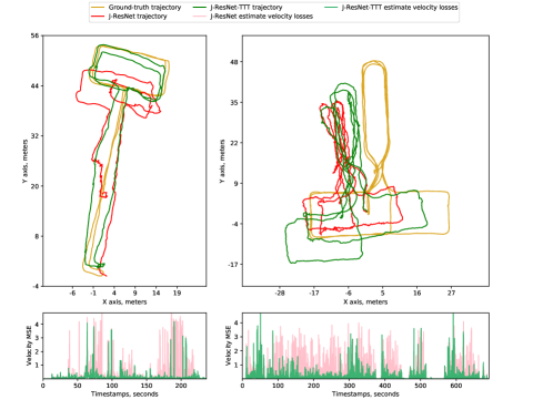
Figure 3: Comparison of example trajectories. The left is a trajectory from IPS database and the right is from RoNIN. For both, TTT strategy based on rotation-equivariance descreased velocity MSE and resulted in better trajectory estimations. More examples are in the appendix.

Network details We adopt Resnet-18 backbone since ResNet-18 model achieved the highest accuracy on multiple datasets shown by RoNIN. We replace Batch Normalization (BN) with Group Normalization (GN) in that the trained model is going to be used in TTT where training with small batches. BN that uses estimated batch statistics has been shown to be ineffective with small batches whose statistics are not accurate. GN that uses channels group statistics is not influenced by batch size and results in similar results as BN on inertial odometry problem. As we propose in Sec. 3.2, we train a model denoted as J-ResNet with joint-training setting following Algorithm 1.

We use the RoNIN model with ResNet-18 backbone as a baseline. While RoNIN publish a pre-trained ResNet model, denoted as R-ResNet, which is exactly the one they claimed in [12], it is a model using BN and trained with the whole RoNIN dataset. They only publish half of the whole database due to privacy limitation. For fair comparison, we re-train a model using GN with the public database as a baseline. Other implementations are exactly the same as they claimed in [12]. We denote the re-trained model as B-ResNet.

Databases Models are evaluated with three popular public databases for inertial odometry: OXIOD[6], RoNIN[12] and RIDI[31], and one database collected in different scenarios by ourselves, IPS. Collecting details are presented in the supplementary. For trajectory sequences in OXIOD RIDI and IPS, the whole estimated trajectory is aligned to the ground-truth trajectory with Umeyama algorithm [27] before evaluation. For RoNIN whose sensor data and ground-truth trajectory data are well calibrated to the same global frame, we directly use the reconstructed trajectory to compare with the ground-truth.

We evaluate neural networks J-ResNet and B-ResNet with two different approaches. One is the standard neural network inference pipeline which is the same as in IONet[4], RoNIN[12], and another use the adaptive TTT proposed in Sec. 3.3. R-ResNet is evaluated only with standard pipeline since it is with BN as normalization layers and it cannot be optimized with small data batch.

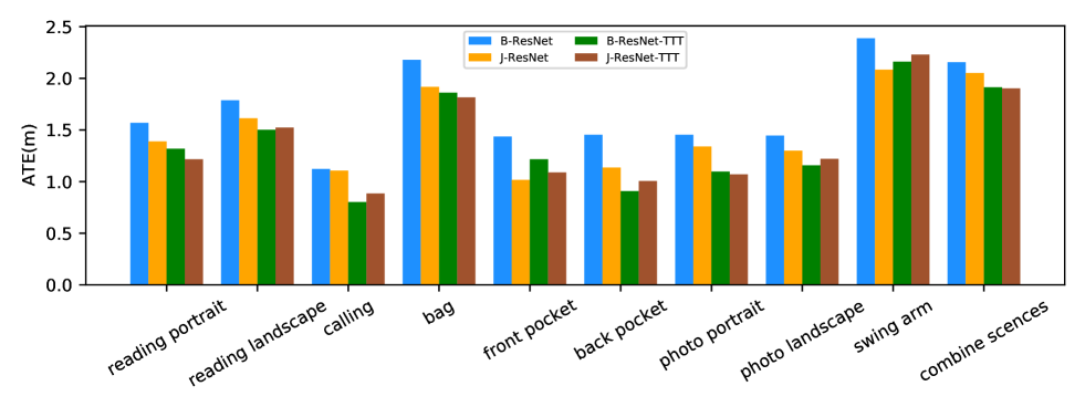
Figure 4: Comparison of performance on different scenarios included in IPS database. In most scenarios, models with TTT strategy have a better performance and J-ResNet is better than B-ResNet.

4.1 Metrics definitions

Three metrics are used for quantitative trajectory evaluation of inertial odometry model: Absolute Trajectory Error (ATE) and Relative Trajectory Error (RTE), and Distance drift (D-drift). ATE and RTE are standard metrics proposed in [23].

ATE ($m$), is calculated as the average Root Mean Squared Error (RMSE) between the estimated and ground-truth trajectories as a whole.

RTE ($m$), is calculated as the average RMSE between the estimated and ground-truth over a fixed length or time interval. Here we use time-based RTE the same as in RoNIN that we evaluate RTE over 1 minute.

D-drift, is calculated as absolute difference between the estimated and ground-truth trajectory length divided by the length of ground-truth trajectory.

4.2 Performance

Tab. 1 is our main results. All subjects used to evaluate models do not present in training sets. Our evaluation of the R-ResNet for RoNIN test datasets is consistent with the report of RoNIN unseen sets in [12]. Other three datasets are not used in the training phase. R-ResNet is trained with full RoNIN dataset and we only use half of it which is published to train B-ResNet and J-ResNet. Therefore, we evaluate R-ResNet performance just for reference. B-ResNet is a fair baseline and we compare other methods with it.

The results show that J-ResNet outperforms B-ResNet on most databases. J-ResNet reduces ATE by $9.96\%$, $4.47\%$ and $9.13\%$ on RoNIN, RIDI and IPS databases, respectively. Notably, for RoNIN database, J-ResNet outperforms R-ResNet which is trained with twice as much training data.

B-ResNet-TTT outperforms B-ResNet on all databases by a significant margin. It reduces ATE by $9.29\%$, $17.04\%$, $11.84\%$ and $15.59\%$ on RoNIN, RIDI, OXIOD and IPS databases, respectively. For J-ResNet-TTT, it reduces ATE by $17.55\%$, $9.43\%$ and $7.06\%$ on OXIOD, RIDI and IPS, and it has a comparable performance on RoNIN comparing to J-ResNet. In a word, the adaptive TTT strategy proposed in Sec. 3.3 can further improve performance of B-ResNet and J-ResNet.

Both models are trained with RoNIN training database in training phase. J-ResNet is trained with the auxiliary task and it already helps to improve performance on RoNIN test database. We assume the auxiliary task is optimized in training phase for RoNIN database that it does not significant improve model performance further with test-time training. For OXIOD, RIDI and IPS which are novel databases for both models, adaptive TTT further improve models performance on all metrics.

Fig. 3 shows selected trajectories performance visualization of J-ResNet and J-ResNet-TTT. It shows estimate trajectories against the ground-truth of both models along with velocity estimation losses comparison. Velocity estimation losses are reduced a lot when there are large velocity losses of original model. It demonstrates that the auxiliary task used in adaptive TTT can help to optimize model at pivotal steps and result in a better trajectory estimation.

4.3 Performance on Multiple Scenarios

The proposed rotation-equivariance contributes differently in different scenarios. Although RoNIN training database is the largest public inertial odometry database with rich diversity, model performance under certain scenarios can be improved by a large margin using RIO.

We compare model performance by scenarios in IPS database and present results in Fig. 4. In different scenarios, devices with IMU sensors are mounted at different placements, and are handled with different ways. Fig. 4 shows that in all scenarios, J-ResNet outperforms B-ResNet, and TTT version of both models improve even further. Under calling, back pocket, photo portrait and photo landscape scenarios, ATE of B-ResNet can be reduced by $28.55\%$, $37.56\%$, $24.47\%$ and $19.92\%$, and for J-ResNet, TTT version reduces ATE by $20.06\%$, $11.36\%$, $20.13\%$ and $6.02\%$, respectively. These four scenarios are not very common in daily life and may not show up as frequent as other poses in RoNIN training database. Therefore, large improvements under unusual scenarios elucidate that adaptive TTT helps trained models to learn from novel data distribution and improve their performance under distribution shifts.

4.4 TTT Strategy Analysis

In this section, we evaluate the TTT strategy in isolation and explain why uncertainty estimations help with model performance improvement.

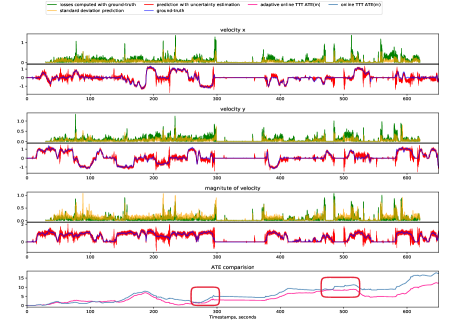
Figure 5: Example of the uncertainty estimation. Estimated velocity uncertainty well follows estimation errors. Adaptive TTT using uncertainty estimations leads to a lower ATE as the model is updated. More examples are in the appendix.

Database	Metric	A-TTT	N-TTT
RoNIN	ATE ($m$)	5.05	4.94
	RTE ($m$)	4.14	4.27
	D-drift	8.49$\%$	9.43$\%$
OXIOD	ATE ($m$)	2.92	3.50
	RTE ($m$)	3.67	4.39
	D-drift	15.50$\%$	19.55$\%$
RIDI	ATE ($m$)	1.04	1.11
	RTE ($m$)	1.53	1.64
	D-drift	6.89$\%$	7.56$\%$
IPS	ATE ($m$)	1.55	1.63
	RTE ($m$)	1.46	1.54
	D-drift	5.93$\%$	6.73$\%$

Table 2: TTT strategies comparision. A-TTT has an obvious advantage over N-TTT for all metrics on four databases.

1) Is uncertainty estimation with deep ensemble reliable? Fig. 5 shows one trajectory velocity estimations against its ground-truth together with their uncertainty estimations and velocity estimation losses. It demonstrates that our predictive uncertainty well follows the estimation losses. As we expected, the predictive uncertainty decreases when velocity estimation losses decrease. With the uncertainty estimation, we can stop updating when it is below a certain level since the model is pretty accurate at this time. Notably, the predictive uncertainty decreases to zero when the magnitude of velocity is around zero. As mentioned in Sec. 3.3, detection of stationary or nearly stationary zones is important for adaptive TTT in that it is the right time to restore original model parameters.

2) Comparing adaptive TTT with others: Last row of Fig. 5 compares Adaptive TTT (A-TTT) ATE change over time with Naive TTT (N-TTT). N-TTT refers to the process that always update models according to losses of self-supervised task and ignore velocity uncertainty estimations. It keeps the latest updated model and does not restore original parameters over one continuous trajectory. Fig. 5 shows that ATE of N-TTT increase faster than A-TTT. There are two obvious time windows that ATE increase steeper with N-TTT, and during these time velocity is decreasing to zeros which means object is going to be stationary. With adaptive strategy, the model will restore original parameters and ATE will be suppressed. Tab. 2 compares A-TTT and N-TTT on four databases and shows that the performance of A-TTT has obvious advantages over N-TTT.

5 Ablation Studies

We conducted additional experiments with joint-training and TTT settings under ablation considerations.

Models performance v.s. size of training data We trained models in joint-training with different size of training datasets. Denote the neural network which is provided and published by RoNIN[12] as 100% B-ResNet since it is trained with the whole RoNIN database. We trained models with 50%, 30% and 10% data of the whole database in two ways as mentioned before, and evaluate their performance under different settings. Fig. 6 shows the comparison of different models. While B-ResNet and J-ResNet performances drop a lot as the training database becomes smaller, J-ResNet-TTT with 30% training database is still comparable to 100% B-ResNet. However, J-ResNet-TTT performance also drops a lot when using 10% training databases.

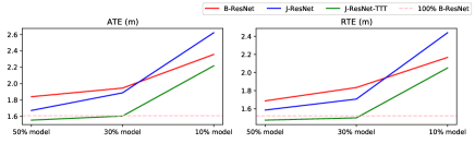
Figure 6: Impact of the size of training data on ATE and RTE. Methods are evaluated on IPS database and compare them with the performance of 100% B-ResNet.

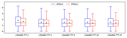
Figure 7: Impact of the number of TTT iterations on ATE and RTE. Methods are evaluated on IPS database.

Influence of updating iterations At test-time, model can be updated multiple times with one batch of data. Fig. 7 shows results of one model with different updating iterations from 1 to 15. There are obvious improvements when increase iterations from 1 to 5. However, more than 5 updates do not show obvious advantages and the model performance even degrade a little when updating 15 times one batch. More iterations cost more time and computing resource. Therefore, we recommend no more than 5 updates one batch during TTT.

6 Discussion and Conclusion

In this paper we present a Rotation-equivariance-supervised Inertial Odometry (RIO) in order to improve performance and robustness of inertial odometry. The rotation-equivariance can be formulated as a self-supervised auxiliary task and can be applied both in training phase and inference stage. Extensive experiments results demonstrate that the rotation-equivariance task helps with advancing model performance under joint-training setting and will further improve model with Test-Time Training (TTT) strategy. Not only rotation-equivariance, there may be more equivariance (e.g., time reversal, mask auto-encoder of time series) that can be formulated as self-supervised task for inertial odometry. We hope our observation will enlighten future work in the aspect of self-supervise learning of inertial odometry.

Further, we propose to employ deep ensemble to estimate the uncertainty of RIO. With uncertainty estimation, we develop adaptive TTT for evolving RIO at inference time. It thus can largely improve the generalizability of RIO. Adaptive TTT using the auxiliary task makes a model trained with less than one-third of the data outperforms the state-of-the-art deep inertial odometry model, especially under scenarios that the model does not see during the training phase. Adaptive online model update with uncertainty estimation is a practical way to improve deep model performance in real life applications. Uncertainty estimation based on deep ensemble gives reliable judgment on the output of deep models. Adaptive TTT can be implemented in different ways, either conservative or aggressive, for updating the model depending on the application scenarios.

Supplementary Materials

Models performance v.s. size of training data We trained models in joint-training setting with different size of training datasets. Denote the neural network which is provided and published by RONIN as 100% B-ResNet since it is trained with the whole RONIN database. We trained models with 50%, 30% and 10% data of the whole database in two ways as mentioned before. And evaluate their performance under different settings. Fig. 6 shows the comparison of different models. While B-ResNet and J-ResNet performances drop a lot as the training database becomes smaller, J-ResNet-TTT with 30% training database is still comparable to 100% B-ResNet. However, J-ResNet-TTT performance also drops a lot when using 10% training databases.

Influence of updating iterations At test-time, model can be update multiple times with one batch of data. Fig. 7 shows results of one model with different updating iterations from 1 to 15. There are obvious improvements when increase iterations from 1 to 5. However, more than 5 updates do not show obvious advantages and the model performance even degrade a little when updating 15 times one batch. More iterations cause more time and computing resource consumption. Therefore, we recommend no more than 5 updates one batch during TTT.

At test-time, model can be update multiple times with one batch of data. Fig. 7 shows results of one model with different updating iterations from 1 to 15. There are obvious improvements when increase iterations from 1 to 5. However, more than 5 updates do not show obvious advantages and the model performance even degrade a little when updating 15 times one batch. More iterations cause more time and computing resource consumption. Therefore, we recommend no more than 5 updates one batch during TTT.

Influence of updating iterations At test-time, model can be update multiple times with one batch of data. Fig. 7 shows results of one model with different updating iterations from 1 to 15. There are obvious improvements when increase iterations from 1 to 5. However, more than 5 updates do not show obvious advantages and the model performance even degrade a little when updating 15 times one batch. More iterations cause more time and computing resource consumption. Therefore, we recommend no more than 5 updates one batch during TTT.

At test-time, model can be update multiple times with one batch of data. Fig. 7 shows results of one model with different updating iterations from 1 to 15. There are obvious improvements when increase iterations from 1 to 5. However, more than 5 updates do not show obvious advantages and the model performance even degrade a little when updating 15 times one batch. More iterations cause more time and computing resource consumption. Therefore, we recommend no more than 5 updates one batch during TTT.

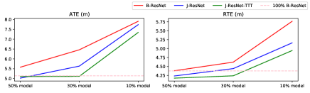
Figure 8: Impact of the number of TTT iterations on ATE and RTE

Figure 9: Impact of the number of TTT iterations on ATE and RTE

Figure 10: Impact of the number of TTT iterations on ATE and RTE

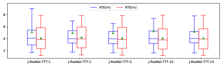
Figure 11: Impact of the number of TTT iterations on ATE and RTE

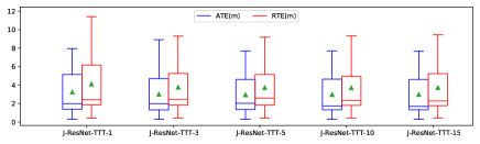
Figure 12: Impact of the number of TTT iterations on ATE and RTE

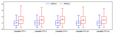
Figure 13: Impact of the number of TTT iterations on ATE and RTE

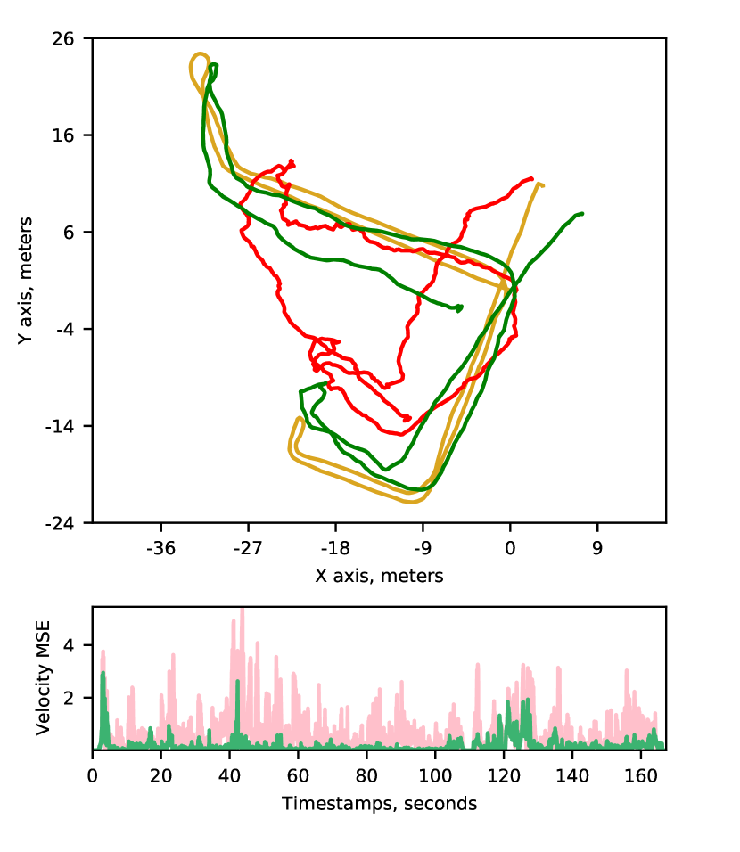
(a) RIDI trajectory1

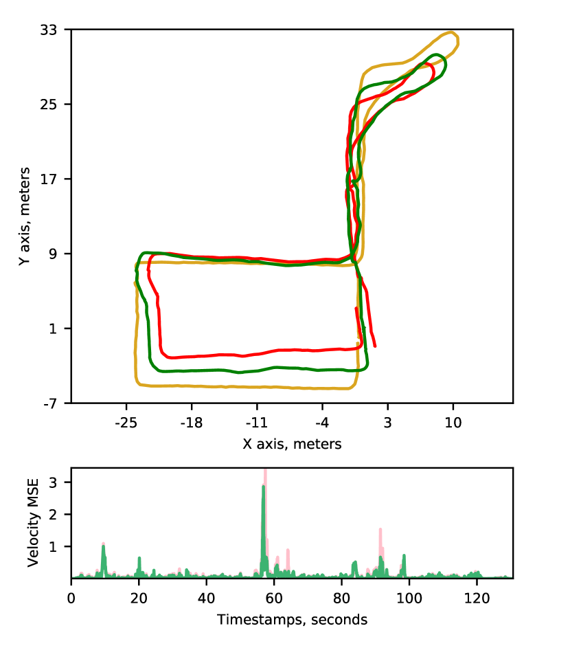
(b) RIDI trajectory2

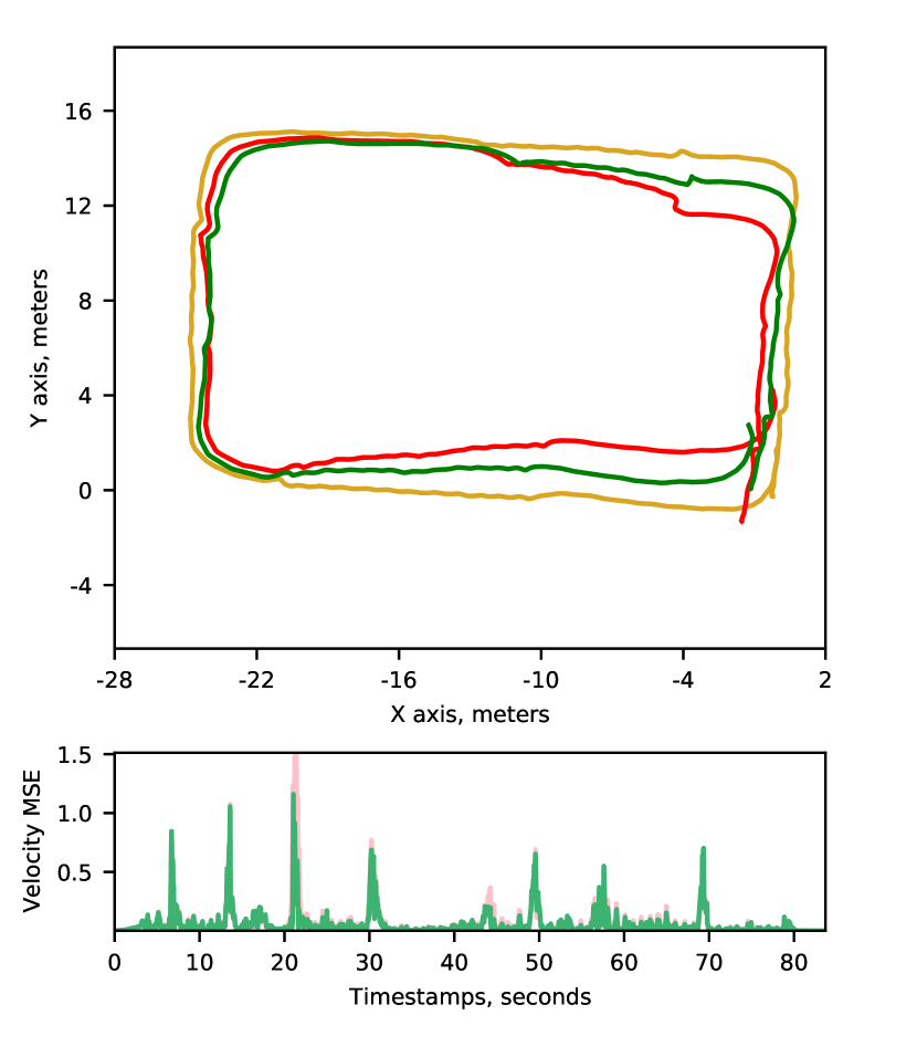
(c) RIDI trajectory3

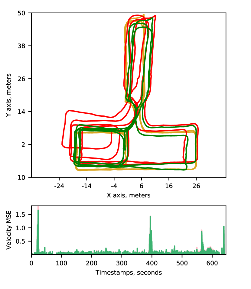
(d) RoNIN trajectory1

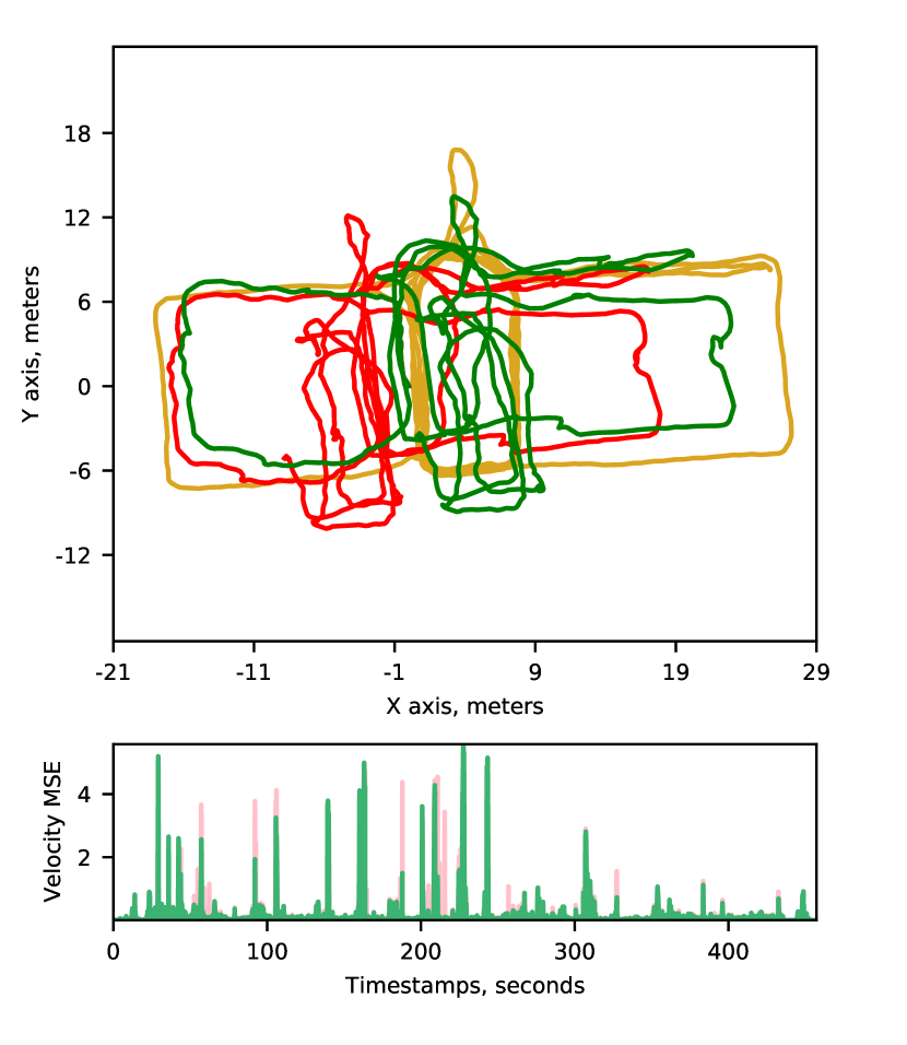
(e) RoNIN trajectory2

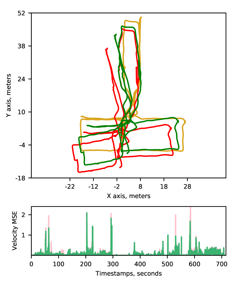
(f) RoNIN trajectory3

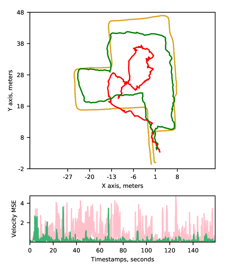
(g) OXIOD trajectory1

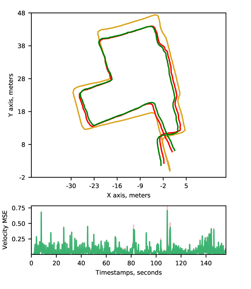
(h) OXIOD trajectory2

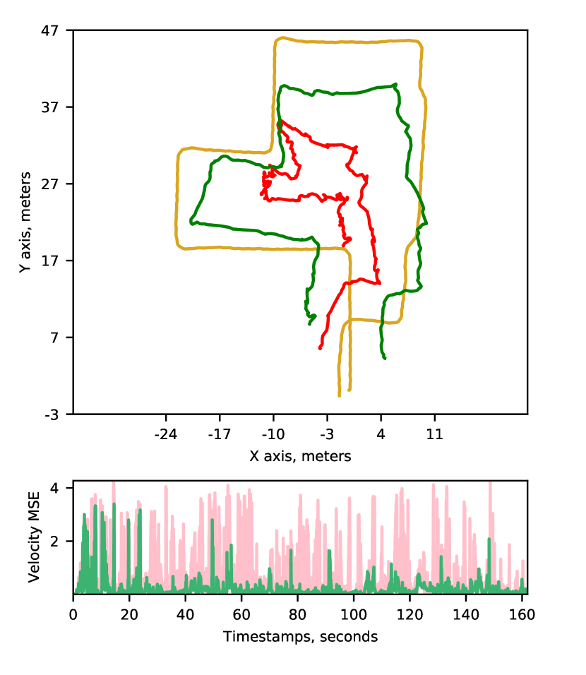
(i) OXIOD trajectory3

Figure 14: Selected visualizations. We select 3 examples from each open sourced dataset and visualize trajectories of ground-truth, J-ResNet and J-ResNet-TTT, along with velocity losses comparison of J-ResNet and J-ResNet-TTT.

References

- [1] Pulkit Agrawal, Joao Carreira, and Jitendra Malik. Learning to see by moving. In Proceedings of the IEEE international conference on computer vision, pages 37–45, 2015.
- [2] Omri Asraf, Firas Shama, and Itzik Klein. Pdrnet: A deep-learning pedestrian dead reckoning framework. IEEE Sensors Journal, 2021.
- [3] John E Bortz. A new mathematical formulation for strapdown inertial navigation. IEEE transactions on aerospace and electronic systems, (1):61–66, 1971.
- [4] Changhao Chen, Xiaoxuan Lu, Andrew Markham, and Niki Trigoni. Ionet: Learning to cure the curse of drift in inertial odometry. In Proceedings of the AAAI Conference on Artificial Intelligence, volume 32, 2018.
- [5] Changhao Chen, Yishu Miao, Chris Xiaoxuan Lu, Linhai Xie, Phil Blunsom, Andrew Markham, and Niki Trigoni. Motiontransformer: Transferring neural inertial tracking between domains. In Proceedings of the AAAI Conference on Artificial Intelligence, volume 33, pages 8009–8016, 2019.
- [6] Changhao Chen, Peijun Zhao, Chris Xiaoxuan Lu, Wei Wang, Andrew Markham, and Niki Trigoni. Oxiod: The dataset for deep inertial odometry. arXiv preprint arXiv:1809.07491, 2018.
- [7] Xinlei Chen and Kaiming He. Exploring simple siamese representation learning. In Proceedings of the IEEE/CVF Conference on Computer Vision and Pattern Recognition, pages 15750–15758, 2021.
- [8] Christian Forster, Luca Carlone, Frank Dellaert, and Davide Scaramuzza. On-manifold preintegration for real-time visual–inertial odometry. IEEE Transactions on Robotics, 33(1):1–21, 2016.
- [9] Eric Foxlin. Pedestrian tracking with shoe-mounted inertial sensors. IEEE Computer graphics and applications, 25(6):38–46, 2005.
- [10] Robert Harle. A survey of indoor inertial positioning systems for pedestrians. IEEE Communications Surveys & Tutorials, 15(3):1281–1293, 2013.
- [11] Kaiming He, Xiangyu Zhang, Shaoqing Ren, and Jian Sun. Deep residual learning for image recognition. In Proceedings of the IEEE conference on computer vision and pattern recognition, pages 770–778, 2016.
- [12] Sachini Herath, Hang Yan, and Yasutaka Furukawa. Ronin: Robust neural inertial navigation in the wild: Benchmark, evaluations, & new methods. In 2020 IEEE International Conference on Robotics and Automation (ICRA), pages 3146–3152. IEEE, 2020.
- [13] Ngoc-Huynh Ho, Phuc Huu Truong, and Gu-Min Jeong. Step-detection and adaptive step-length estimation for pedestrian dead-reckoning at various walking speeds using a smartphone. Sensors, 16(9):1423, 2016.
- [14] Roland Hostettler and Simo Särkkä. Imu and magnetometer modeling for smartphone-based pdr. In 2016 International Conference on Indoor Positioning and Indoor Navigation (IPIN), pages 1–8. IEEE, 2016.
- [15] Antonio R Jimenez, Fernando Seco, Carlos Prieto, and Jorge Guevara. A comparison of pedestrian dead-reckoning algorithms using a low-cost mems imu. In 2009 IEEE International Symposium on Intelligent Signal Processing, pages 37–42. IEEE, 2009.
- [16] Nikos Komodakis and Spyros Gidaris. Unsupervised representation learning by predicting image rotations. In International Conference on Learning Representations (ICLR), 2018.
- [17] Balaji Lakshminarayanan, Alexander Pritzel, and Charles Blundell. Simple and scalable predictive uncertainty estimation using deep ensembles. arXiv preprint arXiv:1612.01474, 2016.
- [18] Wenxin Liu, David Caruso, Eddy Ilg, Jing Dong, Anastasios I Mourikis, Kostas Daniilidis, Vijay Kumar, and Jakob Engel. Tlio: Tight learned inertial odometry. IEEE Robotics and Automation Letters, 5(4):5653–5660, 2020.
- [19] Alejandro Newell and Jia Deng. How useful is self-supervised pretraining for visual tasks? In Proceedings of the IEEE/CVF Conference on Computer Vision and Pattern Recognition (CVPR), June 2020.
- [20] Sang Kyeong Park and Young Soo Suh. A zero velocity detection algorithm using inertial sensors for pedestrian navigation systems. Sensors, 10(10):9163–9178, 2010.
- [21] Zhongzheng Ren and Yong Jae Lee. Cross-domain self-supervised multi-task feature learning using synthetic imagery. In Proceedings of the IEEE Conference on Computer Vision and Pattern Recognition, pages 762–771, 2018.
- [22] Arno Solin, Santiago Cortes, Esa Rahtu, and Juho Kannala. Inertial odometry on handheld smartphones. In 2018 21st International Conference on Information Fusion (FUSION), pages 1–5. IEEE, 2018.
- [23] Jürgen Sturm, Nikolas Engelhard, Felix Endres, Wolfram Burgard, and Daniel Cremers. A benchmark for the evaluation of rgb-d slam systems. In 2012 IEEE/RSJ international conference on intelligent robots and systems, pages 573–580. IEEE, 2012.
- [24] Scott Sun, Dennis Melamed, and Kris Kitani. Idol: Inertial deep orientation-estimation and localization. arXiv preprint arXiv:2102.04024, 2021.
- [25] Yu Sun, Xiaolong Wang, Zhuang Liu, John Miller, Alexei Efros, and Moritz Hardt. Test-time training with self-supervision for generalization under distribution shifts. In International Conference on Machine Learning, pages 9229–9248. PMLR, 2020.
- [26] David Titterton, John L Weston, and John Weston. Strapdown inertial navigation technology, volume 17. IET, 2004.
- [27] Shinji Umeyama. Least-squares estimation of transformation parameters between two point patterns. IEEE Transactions on Pattern Analysis & Machine Intelligence, 13(04):376–380, 1991.
- [28] Xi Wang, Mingxing Jiang, Zhongwen Guo, Naijun Hu, Zhongwei Sun, and Jing Liu. An indoor positioning method for smartphones using landmarks and pdr. Sensors, 16(12):2135, 2016.
- [29] Yingying Wang, Hu Cheng, Chaoqun Wang, and Max Q-H Meng. Pose-invariant inertial odometry for pedestrian localization. IEEE Transactions on Instrumentation and Measurement, 70:1–12, 2021.
- [30] Yuanxin Wu, Xiaoping Hu, Dewen Hu, Tao Li, and Junxiang Lian. Strapdown inertial navigation system algorithms based on dual quaternions. IEEE transactions on aerospace and electronic systems, 41(1):110–132, 2005.
- [31] Hang Yan, Qi Shan, and Yasutaka Furukawa. Ridi: Robust imu double integration. In Proceedings of the European Conference on Computer Vision (ECCV), pages 621–636, 2018.
- [32] Baoding Zhou, Zhining Gu, Wei Ma, and Xu Liu. Integrated ble and pdr indoor localization for geo-visualization mobile augmented reality. In 2020 16th International Conference on Control, Automation, Robotics and Vision (ICARCV), pages 1347–1353. IEEE, 2020.
- [33] Caifa Zhou, Zhi Li, Dandan Zeng, and Yongliang Wang. Mining geometric constraints from crowd-sourced radio signals and its application to indoor positioning. IEEE Access, 9:46686–46697, 2021.
- [34] Tinghui Zhou, Matthew Brown, Noah Snavely, and David G. Lowe. Unsupervised learning of depth and ego-motion from video. In Proceedings of the IEEE Conference on Computer Vision and Pattern Recognition (CVPR), July 2017.