Physical and geometrical parameters of CVBS XIV: The two nearby systems HIP 19206 and HIP 84425

Abstract

The data release DR2 of Gaia mission was of great help in precise determination of fundamental parameters of Close Visual Binary and Multiple Systems (CVBMSs), especially masses of their components, which are crucial parameters in understating formation and and evolution of stars and galaxies. This article presents the complete set of fundamental parameters of two nearby (CVBSs), these are HIP 19206 and HIP 84425. We used a combination of two methods; the first one is Tokovinin’s dynamical method to solve the orbit of the system and to estimate orbital elements and the dynamical mass sum, and the second one is Al-Wardat’s method for analyzing CVBMSs to estimate the physical parameters of the individual components. The latest method employs grids of Kurucz line-blanketed plane parallel model atmospheres to build synthetic Spectral Energy Distributions (SED) of the individual components. Trigonometric parallax measurements given by Gaia DR2 and Hipparcos catalogues are used to analyse the two systems. The difference in these measurements yielded slight discrepancies in the fundamental parameters of the individual components especially masses. So, a new dynamical parallax is suggested in this work based on the most convenient mass sum as given by each of the two methods. The new dynamical parallax for the system Hip 19205 as $22.97\pm 0.95$ mas coincides well with the trigonometric one given recently (in December 2020) by Gaia DR3 as $22.3689\pm 0.4056$ mas. The positions of the components of the two systems on the evolutionary tracks and isochrones are plotted, which suggest that all components are solar-type main sequence stars. Their most probable formation and evolution scenarios are also discussed.

1 Introduction

The study of the physical and geometrical parameters, especially masses, of close visual binary systems (CVBSs) plays an important role in revealing the secrets of formation and evolution of such systems, and hence the formation and evolution of the Galaxy. It also represents a direct tool for the investigation of laws and rules of astrophysics.

The preciseness of such studies is highly enhanced by the latest measurements of the distances to such systems, which were highly achieved by Gaia astrometric mission [Collaboration et al.(2018), Al-Wardat et al.(2021)].

The two systems under study fulfill the following specific requirements; The two components of the system are visually close enough that they can not be observed and studied individually, and the system has available accurate measurements of its colours, colour indices and magnitude difference between its components.

The study uses two complementary methods; Tokovinin’s dynamical method for the orbital solutions, and Al-Wardat’s complex method for analyzing CVBMSs.

Al-Wardat’s method is an indirect computational spectrophotmetrical method that uses the available observations (magnitudes and magnitude differences) of a binary or a multiple system to build a synthetic Spectral Energy Distribution (SED) for each individual component. It employs grids of Kurucz’s line-blanketed plane parallel atmospheres to build these synthetic SEDs  [Kurucz(1994)]. Then it combines these SEDs depending on some geometrical information like the system’s parallax and the radii of the components to get the entire SED of the system, from which we can calculate the synthetic magnitudes and colour indices. This process is subject to iteration until the best fit between the synthetic and observational magnitudes and colour indices are achieved. Whereupon, input parameters, both those of the model atmospheres and the geometrical calculations, represent the fundamental parameters of the system adequately enough within the error values of the measured ones.

This methods was successfully applied to several CVBMSs. Some of them were solar type stars, while the others were found to be subgiant stars.

The criterion of the judgement of Al-Wardat’s method is the best fit between the observational entire colours and colour indices with the synthetic ones. In the case of the existence of the entire observational SED, it is usually used as an additional judgement tool by achieving the best fit with the synthetic one.

Of the solar type CVBSs which studied using Al-Wardat’s method we mention here: ADS 11061, COU 1289, COU 1291, HIP 11352, HIP 11253, HIP 70973, HIP 72479, Gliese 150.2, Gliese 762.1, COU 1511, FIN 350, and HIP 109951 (see i.e. [Al-Wardat(2002), Al-Wardat(2007), Al-Wardat(2009), Al-Wardat(2012), Al-Wardat et al.(2014a), Al-Wardat et al.(2016), Masda et al.(2016), Al-Wardat et al.(2017), Masda et al.(2019), Masda et al.(2019)]. Of course, the method can deduce if the system is evolved or not!, here are some evolved (sub-giants) CVBSs which were analyzed using the method; HD 25811, HD 375 and HD 6009 (see i.,e. [Al-Wardat et al.(2014b), Al-Wardat(2014), Al-Wardat et al.(2014a)] for full details and references).

This paper presents the analysis of two nearby CVBSs; these are HIP 19206 (HD 26040) and HIP 84425 (HD 155826).

2 Archived data

The observational photometric data are taken from reliable different sources, such as the old Hipparcos Catalogue [ESA(1997)], new Hipparcos reduction [van Leeuwen(2007)] and Gaia data release 2 (DR2) [Collaboration et al.(2018)].

Table 1: Observational data for HIP 19206 and HIP 84425.

Hip	19206	84425	Source of data
HD	26040	155826
$\alpha_{2000}$	$04^{\rm h}07^{\rm m}00^{\rm s}566$	$17^{\rm h}15^{\rm m}35^{\rm s}902$	SIMBAD1
$\delta_{2000}$	$-10\degr 00^{\prime}01.^{\prime\prime}857$	$-38\degr 35^{\prime}38.^{\prime\prime}902$	-
Sp. Typ.	G1/2V	G0V	-
$A_{V}$	$0.0$	$0.0062$	[Lallement et al.(2018)]
$V_{J}(Hip)$	6.88	5.95	[ESA(1997)]
$(V-I)_{J}$	$0.65\pm 0.00$	$0.64\pm 0.02$	-
$(B-V)_{J}$	$0.576\pm 0.004$	$0.580\pm 0.004$	-
$B_{T}$	$7.566\pm 0.008$	$6.67\pm 0.013$	-
$V_{T}$	$6.957\pm 0.006$	$6.015\pm 0.006$	-
$\pi_{Hip}$ (mas)	$24.00\pm 0.92$	$32.6\pm 1.7$	-
$\pi_{Hip}$ (mas)	$24.49\pm 0.83$	$32.69\pm 0.59$	Van Leeuwen 2007
$\pi_{Gaia}$ (mas)	$23.4039\pm 0.4727$	$30.4039\pm 0.4728$	[Collaboration et al.(2018)]

Notes.
¹ http://simbad.u-strasbg.fr/simbad/sim-fid.

These data are used to calculate the preliminary input parameters and as reference for the best fit with the synthetic photometry. Table 1 contains the catalogued data for HIP 19206 and HIP 84425. These data were taken from SIMBAD database, the Hipparcos and Tycho Catalogues and Gaia DR2. For the orbital solutions, we used data from the Fourth Catalog of Interferometric Measurements of Binary Stars [Hartkopf et al.(2001)].

3 Methods and Analysis

3.1 Orbital solutions

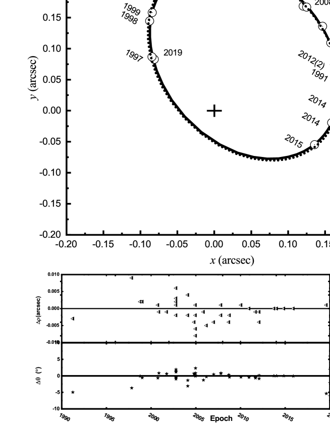
Figure 1: The modified orbit of the HIP 19206 system as determined from our analysis (solid line) and last orbit from ORB6 (dotted line). The bottom left panel shows the fit residuals, showing the difference between the observed and model values for the angular separation ($\Delta\rho$) and position angle ($\Delta\theta$) of the orbit. The bottom right panel represents the distribution of data based on a five-number summary (”minimum” first quartile (Q1); median, third quartile (Q3); and ”maximum”) and outliers.

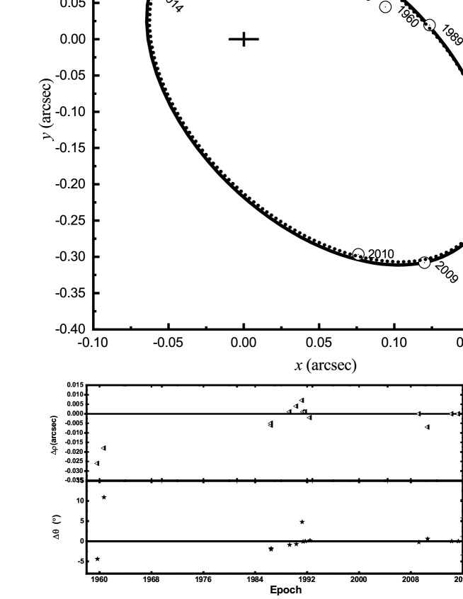
Figure 2: The modified orbit of the HIP 84425 system as determined from our analysis (solid line) and last orbit from ORB6 (dotted line). The bottom left panel shows the fit residuals, showing the difference between the observed and model values for the angular separation ($\Delta\rho$) and position angle ($\Delta\theta$) of the orbit. The bottom right panel represents the distribution of data based on a five-number summary (”minimum” first quartile (Q1); median, third quartile (Q3); and ”maximum”) and outliers.

For the orbital solution and modification of the orbital elements of the systems, we follow Tokovinin’s dynamical method using the ORBITX code of [Tokovinin et al.(2016)]. We used the relative position measurements; angular separations ($\rho$) in ($\arcsec$) and position angles ($\theta$) in ($\deg$) obtained by different observational techniques and listed in the Fourth Catalog of Interferometric Measurements of Binary Stars (INT4). The program performs a least-squares adjustment to all available relative position observations, with weights inversely proportional to the square of their standard errors.

The orbital solution involves the orbital period $P$ (in years); the eccentricity e, the semi-major axis $a$ (in arcsecond), the inclination $\rm i$ (in degree), the argument of periastron $\rm\omega$ (in degree), the position angle of nodes $\rm\Omega$ (in degree), and the time of periastron passage $\rm T_{0}$ (in years).

HIP 19206; the Preliminary orbital parameters of the system were calculated by [Balega et al.(2006b)], then modified two times by [Tokovinin et al.(2015)] and [Tokovinin(2019)].

In this work, we use 41 points of positional measurements ($\rho$) and ($\theta$) covers the period from 1991 to 2019. The latest points are published by: [Tokovinin et al.(2015)] (one point), [Mason et al.(2018)](3-points), and [Tokovinin(2019)] (one point).

Table 2: Modified orbital elements, mass sums, and quality controls of the system HIP 19206 obtained in this work, along with previous ones of: (1) [Balega et al.(2006b)], (2) [Tokovinin et al.(2015)] and (3) [Tokovinin(2019)].

		System HIP 19206
Parameters	Units	(1)	(2)	(3)	This work
$P\pm\sigma_{P}$	[yr]	$21.33\pm 0.44$	$21.42\pm 0.037$	21.06	$21.103\pm 0.00$
$T_{0}\pm\sigma_{T_{0}}$	[yr]	$1996.77\pm 0.08$	$1996.78\pm 0.06$	2017.94	$1996.91\pm 0.00$
$e\pm\sigma_{\rm e}$	-	$0.686\pm 0.011$	$0.687\pm 0.009$	0.711	$0.7019\pm 0.00$
$a\pm\sigma_{\rm a}$	[arcsec]	$0.223\pm 0.006$	$0.225\pm 0.006$	0.229	$0.226\pm 0.000$
$i\pm\sigma_{\rm i}$	[deg]	$122.2\pm 1.2$	$122.9\pm 1$	121.7	$122.68\pm 0.00$
${\Omega}\pm\sigma_{\rm{\Omega}}$	[deg]	$255.6\pm 1.1$	$219.0\pm 1.8$	220.4	$219.00\pm 0.08$
$\omega\pm\sigma_{\rm\Omega}$	[deg]	$38.2\pm 1.7$	$76.4\pm 0.5$	77.3	$76.40\pm 0.05$
$\rm M_{dyn}{\pm\sigma_{\rm M}}^{1}$	[M⊙]	$1.763\pm 0.258$	$1.796\pm 0.252$	$1.959$	$1.873\pm 0.215$
$\rm M_{dyn}{\pm\sigma_{\rm M}}^{2}$	[M⊙]	$1.659\pm 0.226$	$1.690\pm 0.219$	$1.843$	$1.762\pm 0.179$
$\rm M_{dyn}{\pm\sigma_{\rm M}}^{3}$	[M⊙]	$1.965\pm 0.215$	$2.001\pm 0.202$	$2.183$	$2.087\pm 0.128$
$rms(\theta)$	[deg]	0.9	0.2335		0.10
$rms(\rho)$	[arcsec]	0.002	0.9268		0.0002

Notes.
¹ Using ($\pi_{Hip1997}$), ² Using ($\pi_{Hip2007}$)
³ Using ($\pi_{Gaia2018}$).

HIP 84425; the Preliminary orbital parameters of the system were calculated by [Söderhjelm(1999)] then modified two times by [Rica Romero(2010)] and [Tokovinin et al.(2015)].

Table 3: Modified orbital elements, mass sums, and quality controls of the system HIP 84425, along with previous ones of: (1) [Söderhjelm(1999)], (2) [Rica Romero(2010)] , and (3) [Tokovinin et al.(2015)]

		System HIP 84425
Parameter	Units	(1)	(2)	(3)	This work
$P$ $\pm$ $\sigma_{\rm P}$	[yr]	$23.3$	$14.215\pm 0.050$	$14.23\pm 0.03$	$14.247\pm 0.057$
$T_{0}$ $\pm$ $\sigma_{\rm T_{0}}$	[yr]	$1986.5$	$1985.98\pm 0.17$	$1985.97\pm 0.06$	$1985.98\pm 0.15$
$e$ $\pm$ $\sigma_{\rm e}$	-	$0.5$	$0.491\pm 0.005$	$0.476\pm 0.01$	$0.465\pm 0.008$
$a$ $\pm$ $\sigma_{\rm a}$	[arcsec]	$0.28$	$0.253\pm 0.004$	$0.249\pm 0.02$	$0.253\pm 0.002$
$i$ $\pm$ $\sigma_{\rm i}$	[deg]	$123$	$115.2\pm 1.1$	$115.3\pm 0.6$	$115.05\pm 0.75$
$\Omega$ $\pm$ $\sigma_{\rm\Omega}$	[deg]	$4$	$190.41\pm 0.62$	$191.81\pm 0.47$	$192.06\pm 0.37$
$\omega$ $\pm$ $\sigma_{\rm\omega}$	[deg]	$349$	$135.2\pm 2.5$	$137.2\pm 1.0$	$137.24\pm 2.04$
$\rm M_{dyn}{\pm\sigma_{\rm M}}^{1}$	[$M_{\odot}$]	1.17	$2.305\pm 0.379$	$2.201\pm 0.632$	$2.307\pm 0.364$
$\rm M_{dyn}{\pm\sigma_{\rm M}}^{2}$	[$M_{\odot}$]	1.16	$2.286\pm 0.171$	$2.183\pm 0.539$	$2.287\pm 0.133$
$\rm M_{dyn}{\pm\sigma_{\rm M}}^{3}$	[M⊙]	1.45	$2.841\pm 0.197$	$2.713\pm 0.666$	$2.842\pm 0.146$
$rms(\theta)$	[deg]		0.2	1.26	0.06
$rms$ ($\rho$)	[arcsec]		1.0	0.93	0.0001

Notes.
¹ Using ($\pi_{Hip1997}$), ² Using ($\pi_{Hip2007}$)
³ Using ($\pi_{Gaia2018}$).

In this work, we use 16 points of the relative positional measurements ($\rho$) and ($\theta$) from the year 1959 to the year 2015, the latest point was published by [Tokovinin et al.(2016)], and is used for first time in this work.

We calculate the total dynamical mass using Kepler’s third law, where we use the semi-major axis and the period from the orbital solution and the parallax measurements from either Hipparcos [ESA(1997)], Hipparcos 2007 [van Leeuwen(2007)], or Gaia DR2 [Collaboration et al.(2018)].

Kepler’s third law for binary stars can be expressed as follows:

$$\rm M_{dyn}=\rm M_{A}+\rm M_{B}=(\frac{\textit{a}^{3}}{\pi^{3}P^{2}})\rm M_{\odot}$$ (1)

and the formal error is given by

$$\frac{\sigma_{\rm M}}{\rm M}=\sqrt{9(\frac{\sigma_{\pi}}{\pi})^{2}+9(\frac{\sigma_{a}}{a})^{2}+4(\frac{\sigma_{P}}{P})^{2}}.$$ (2)

3.2 Physical parameters

The first step in applying the analysis using Al-Wardat’s method is to determine correctly the magnitude difference between the two components . For the system HIP 19206, we find it $\triangle m=1.4\pm 0.02$ mag, which is the average measurements under the V-band filters (541-551) nm (see Table 4). While for HIP 84425 we find it $\triangle m=1.6\pm 0.16$ mag as the average value of the V-band filters (543-551) nm measurements listed in Table 4.

Table 4: Magnitude difference between the components of both systems; HIP 19206 and HIP 84425. We listed here only the values taken under filters close to the V-band filter.

HIP	$\triangle m$	${\sigma_{\triangle m}}$	Filter ($\lambda/\Delta\lambda$)	Reference
	(mag)		($~{}\rm nm$)
HIP 19206	$1.39$	0.02	$545/20$	[Balega et al.(2007)]
	$1.40$	$*$	$541/88$	[Horch et al.(2008)]
	$1.43$	$*$	$550/40$	–
	$1.45$	$*$	$550/40$	–
	$1.48$	$*$	$550/40$	–
	$1.4$	$*$	$551/22$	[Tokovinin et al.(2010)]
	$1.5$	$*$	$543/22$	[Tokovinin et al.(2016)]
HIP 84425	$1.6$	$*$	$551/22$	[Tokovinin et al.(2010)]
	$1.6$	$*$	$543/22$	[Tokovinin et al.(2015)]
	$1.7$	$*$	$543/22$	[Tokovinin et al.(2016)]

Using the values of $\triangle m$ along with the apparent visual magnitudes of the systems ($m_{v(HIP19206)}=6.88$ mag, $m_{v(HIP84425}=5.95$ mag ) (see Table 1), we calculate the apparent visual magnitudes of individual components using Equs. 3 and 4. The results are: $m_{v}^{A}=7^{m}.14\pm 0.01$ and $m_{v}^{B}=8^{m}.54\pm 0.02$ for HIP 19206, and: $m_{v}^{A}=6^{m}.17\pm 0.03$ and $m_{v}^{B}=7^{m}.77\pm 0.16$ for HIP 84425.

$$m_{v}^{A}=m_{v}+2.5\log(1+10^{-0.4\triangle m}),$$ (3)

$$\centering m_{v}^{B}=m_{v}^{A}+{\triangle m}.\@add@centering$$ (4)

Where we used the following relations to calculate the error values of the apparent visual magnitudes of the individual components of the system:

$$\sigma^{2}_{m^{A}_{v}}={\sigma_{m_{v}}^{2}+(\frac{1}{1+10^{+0.4\triangle m}})^{2}\sigma_{\triangle m}^{2}},$$ (5)

$$\sigma^{2}_{m^{B}_{v}}={\sigma_{m^{A}_{v}}^{2}+\sigma_{\triangle m}^{2}}$$ (6)

As a result, it is found that the absolute visual magnitudes for the primary and secondary components of the systems HIP 19206 are: $M_{V}^{A}=3^{m}.96\pm 0.04$ and $M_{V}^{B}=5^{m}.36\pm 0.05$ respectively, and those for the system HIP 84425 are: $M_{V}^{A}=3^{m}.58\pm 0.05$, $M_{V}^{B}=5^{m}.17\pm 0.03$, using the following equation (Heintz, 1978):

$$M_{V}=m_{v}+5-5\log(d)-A_{V},$$ (7)

Here, the interstellar extinction, $\rm A_{V}$ of HIP 19206 is neglected because this system is a nearby one.

The errors of the absolute visual magnitudes of the components A and B of the system are calculated by using the following equation:

$$\sigma^{2}_{M^{*}_{V}}={\sigma_{m^{*}_{v}}^{2}+(\frac{\log\rm e}{0.2\pi})^{2}\sigma_{\pi}^{2}}~{};~{}~{}~{}~{}~{}\textit{*}=A,B.$$ (8)

where $\sigma_{m^{*}_{v}}$ are the errors of the apparent magnitudes of the A and B components expressed in Equations 5 & 6.

Based on the estimated preliminary absolute magnitudes ($\rm M_{V}$) of the individual components of the two systems, we can find the preliminary values of the effective temperature and the bolometric correction for each component as taken from the Tables of [Gray(2005)] and [Lang(1992)] . For HIP 19206 $T^{A}_{\rm eff}=6160\,\rm K$ ,$T^{B}_{\rm eff}=5550\,\rm K$ and $(B.C)_{\rm A}=-0.12$, $(B.C)_{\rm B}=-0.30$, and for HIP 84425 $T^{A}_{\rm eff}=6520\,\rm K$ ,$T^{B}_{\rm eff}=5650\,\rm K$ and $(B.C)_{\rm A}=-0.12$, $(B.C)_{\rm B}=-0.21$, for the primary and secondary components of the two systems, respectively.

Furthermore, we use Equs. 9,10,11& 12 to calculate the input parameters and to double check them after getting the best fit between the synthetic and observed photometry.

$$M_{bol}=M_{V}+B.C,$$ (9)

$$\log\frac{L}{L_{\odot}}=\frac{M_{bol}^{\odot}-M_{bol}}{2.5},$$ (10)

$$\log\frac{R}{R_{\odot}}=0.5log\frac{L}{L_{\odot}}-2log\frac{T}{T_{\odot}},$$ (11)

$$\log g=\log\frac{\rm M}{\rm M_{\odot}}-2\log\frac{R}{R_{\odot}}+4.43.$$ (12)

where $T_{\odot}=5777\,\rm K$,$R_{\odot}=6.69*10^{\rm 8}\rm m$ and $M_{bol}^{\odot}=4^{\rm m}.75$.

In order to obtain the best stellar parameters, as we mentioned above, we need to build a synthetic SED of the system based on the input parameters and on grids of line-blanketed model atmospheres (ATLAS9) [Kurucz(1994)]. This parameter could not be built unless we are fully aware of the information about its distance d and radius R (see Figures 4 & 5). Hence, the entire synthetic SED as it would be appears at the Earth surface for the entire binary system is related to the individual synthetic SEDs of the components according to the following equation [Al-Wardat(2002), Al-Wardat(2012)]:

$$F_{\lambda}\cdot d^{2}=H_{\lambda}^{A}\cdot R_{A}^{2}+H_{\lambda}^{B}\cdot R_{B}^{2},$$ (13)

where $F_{\lambda}$ is the flux for the entire synthetic SED of the entire binary system at the Earth, $H_{\lambda}^{A}$ and $H_{\lambda}^{B}$ are the fluxes of the primary and secondary components, in units of ergs cm^-2s^-1 Å^-1, while $R_{A}$ and $R_{B}$ are the radii of the primary and secondary components in solar units.

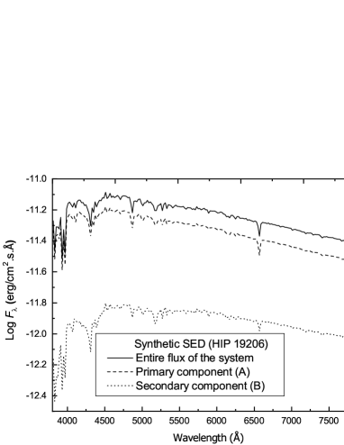
(a) HIP 19206

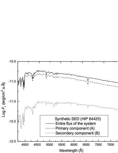
(b) HIP 84425

Figure 3: The entire flux and individual synthetic SEDs of the binary system HIP 19206 and HIP 84425 using Kurucz blanketed models [Kurucz(1994)] (ATLAS9).

Since we do not have observational spectral energy distribution for the systems, we depend on the magnitudes and colour indices as a reference for the best fit with the synthetic ones, which ensures the reliability of the estimated parameters. This technique is a part of Al-Wardat’s complex method for analyzing CVBSs.

4 Synthetic photometry

Stellar parameters depend mainly on the best fit of the magnitudes and color indices between the entire observational and synthetic SED of the system. Therefore, we calculate the individual and total synthetic magnitudes and colour indices of the systems by integrating the total fluxes over each bandpass of the named photometrical system divided by that of the reference star (Vega), using the following equation [Al-Wardat(2012)]:

$$m_{p}[F_{\lambda,s}(\lambda)]=-2.5\log\frac{\int P_{p}(\lambda)F_{\lambda,s}(\lambda)\lambda{\rm d}\lambda}{\int P_{p}(\lambda)F_{\lambda,r}(\lambda)\lambda{\rm d}\lambda}+{\rm ZP}_{p}\,$$ (14)

where $m_{p}$ is the synthetic magnitude of the passband $p$, $P_{p}(\lambda)$ is the dimensionless sensitivity function of the passband $p$, $F_{\lambda,s}(\lambda)$ is the synthetic SED of the object and $F_{\lambda,r}(\lambda)$ is the SED of the reference star (Vega). Zero points (ZP_p) from [Maíz Apellániz(2007)] are used.

Table 5: Magnitudes and colour indices of the entire synthetic spectrum and individual components of HIP 19206 and HIP 84425.

Sys.	Filter	HIP 19206			HIP 84425
		Entire Synth.	A	B	Entire Synth.	A	B
		$\sigma=\pm 0.03$			$\sigma=\pm 0.03$
Joh-	$U$	7.55	7.73	9.62	6.63	6.77	8.95
Cou.	$B$	7.45	7.67	9.33	6.53	6.71	8.58
	$V$	6.88	7.14	8.58	5.95	6.17	7.79
	$R$	6.56	6.84	8.18	5.63	5.87	7.37
	$U-B$	0.09	0.05	0.29	0.10	0.06	0.37
	$B-V$	0.58	0.53	0.75	0.58	0.54	0.79
	$V-R$	0.32	0.93	0.40	0.32	0.93	0.40
Ström.	$u$	8.72	8.89	10.76	7.80	7.94	10.10
	$v$	7.78	7.97	9.73	6.86	7.02	9.01
	$b$	7.21	7.44	8.98	6.28	6.48	8.22
	$y$	6.86	7.11	8.54	5.92	6.14	7.75
	$u-v$	0.94	0.92	1.04	0.95	0.93	1.08
	$v-b$	0.56	0.53	0.74	0.58	0.54	0.79
	$b-y$	0.35	0.33	0.44	0.36	0.34	0.47
Tycho	$B_{T}$	7.59	7.79	0.86	6.67	6.84	8.79
	$V_{T}$	6.95	7.20	8.66	6.02	6.23	7.87
	$B_{T}-V_{T}$	0.65	0.59	0.86	0.65	0.60	0.92

Table 6: Comparison between the observational and synthetic magnitudes and colours indices for both systems.

HIP	Filter	Observed	Synthetic (This work)
		($\rm mag$)	($\rm mag$)
HIP 19206	$V_{J}$	$6.88$	$6.88\pm 0.03$
	$B_{T}$	$7.566\pm 0.008$	7.59$\pm 0.03$
	$V_{T}$	$6.957\pm 0.006$	$6.95\pm 0.03$
	$(B-V)_{J}$	$0.576\pm 0.004$	$0.58\pm 0.03$
	$\triangle m$	$1.4$	$1.4$
HIP 84425	$V_{J}$	$5.95$	$5.95\pm 0.03$
	$B_{T}$	$6.67\pm 0.013$	6.67$\pm 0.03$
	$V_{T}$	$6.015\pm 0.006$	$6.02\pm 0.03$
	$(B-V)_{J}$	$0.58\pm 0.002$	$0.58\pm 0.03$
	$\triangle m$	1.6	1.6

We used the best fit between the observational and synthetic entire magnitudes, magnitude differences of the components ($\triangle m$ = $V^{B}_{J}$-$V^{A}_{J}$) and colour indices to judge the accuracy of the estimated parameters.

The entire flux is calculated from the individual fluxes of the components using Equ. 13  and depending on the parallax of the system.

As mentioned above, we get the color indices of the individual components and entire synthetic SEDs of two systems, in three photometrical systems; Johnson: $U$, $B$, $V$, $R$, $U-B$, $B-V$, $V-R$; Strömgren: $u$, $v$, $b$, $y$, $u-v$, $v-b$, $b-y$ and Tycho: $B_{T}$, $V_{T}$, $B_{T}-V_{T}$, which are listed in Table 5.

5 Results and discussion

Table 5 lists the results of the synthetic magnitudes and colour indices of the entire systems and individual components under three photometric systems: Johnson: $U$, $B$, $V$, $R$, $U-B$, $B-V$, $V-R$; Strömgren: $u$, $v$, $b$, $y$, $u-v$, $v-b$, $b-y$ and Tycho: $B_{T}$, $V_{T}$, $B_{T}-V_{T}$). And Table  6 gives a comparison between the entire synthetic magnitudes and colour indices of the two systems with the available observed ones within three photometric systems. The consistency between the synthetic and observed photometry indicates the reliability of the fundamental parameters of the two systems.

Hereafter we discuss the results of each system separately:

HIP 19206: Table 2 lists the modified orbital elements as per the new orbital solution, which used a total of 41 relative positional measurements, along with the elements of the previous solutions of [Balega et al.(2006a)], [Tokovinin et al.(2015)] and [Tokovinin(2019)]. The RMS values of the new solution $\triangle\rm\theta=0.10\degr$ and $\triangle\rm\rho=0.0002\arcsec$ are better than those of the previous solutions.

Table 7 lists the final fundamental parameters of the system. It shows that the dynamical mass sum of the system using Gaia parallax ($23.4039\pm 0.4727$) is given by $2.087\pm 0.128$ which is the closest to the mass sum given by Al-Wardat’s method as $2.14\pm 0.15$. Which means that Gaia parallax measurement is the best among the other measurements, but in order to achieve the best consistency between the dynamical mass sum and that of Al-Wardat’s method, we propose a new dynamical parallax for the system as $22.97\pm 0.95$ mas.

It is worthwhile to mention here that this work was done before the release of Gaia DR3 in December 2020 which gives a very close trigonometric parallax for the system as $22.3689\pm 0.4056$ mas [Brown et al.(2020)].

The reason why we introduced a new parallax measurement is that parallax measurements of binary and multiple systems are, in some cases, distorted by the orbital motion of the components of such systems as noted by other several researchers (i.e. [Shatskii & Tokovinin(1998)]).

The fundamental parameters of the systems’ components, their positions on the evolutionary tracks of [Girardi et al.(2000)] (Fig. 4a), and on the isochrones of [Girardi et al.(2000)] (Fig 5a), show that they are a twin solar type main sequence stars with a metalicity of 0.019. Which predicts that fragmentation is the most probable formation process for the system.

HIP 84425: Table 3 lists the modified orbital elements as per the new orbital solution, which used a total of 13 relative positional measurements, along with the elements of the previous solutions of [Söderhjelm(1999)], [Rica Romero(2010)] , and [Tokovinin et al.(2015)]. The RMS values of the new solution $\triangle\rm\theta=0.06\degr$ and $\triangle\rm\rho=0.0001\arcsec$ are much better than those of the previous solutions.

Table 8 lists the fundamental parameters of the system as given by Al-Wardat’s method using two parallax measurements; Hipparcos 2007 and Gaia 2018. So, we have to decide which set of parameters represent better the system.

In order to do so, it should be remembered that the dynamical mass sum is highly affected by the parallax, while the masses estimated using Al-Wardat’s method are not as highly affected by the change of the parallax. This is clear in Fig. 4b which shows the positions of the components of HIP 84425 on the evolutionary tracks when using both the parallax given by Hipparcos 2007 and that given by Gaia 2018.

Now, depending on the mass sum of Al-Wardat’s method as $2.2\pm 0.15$ mas, we estimate a new dynamical parallax as ($33.26\pm 1.5$), which is closer to that of Hipparcos 2007 as ($32.69\pm 0.59$). So, we adopt the fundamental parameters given in Table 8 columns 3 and 4.

The fundamental parameters of the systems’ components, their positions on the evolutionary tracks of [Girardi et al.(2000)] (Fig. 4b), and on the isochrones of [Girardi et al.(2000)] (Fig 5b), show that they are a twin solar type in their final main sequence stage with a metalicity of 0.019. Which predicts that fragmentation is the most probable formation process for the system.

Table 7: The fundamental parameters of the individual components of HIP 19206 as estimated using Al-Wardat’s Method.

		HIP 19206
Parameters	Units	HIP 19206 A	HIP 19206 B
$T_{eff}$ $\pm$ $\sigma_{T_{eff}}$	[ K ]	$6300\pm 100$	$5600\pm 100$
$R\pm\sigma_{R}$	[R⊙]	$1.417\pm 0.06$	$0.978\pm 0.05$
$\log\rm g$ $\pm$ $\sigma_{\rm logg}$	[$cm/s^{2}$]	$4.18\pm 0.11$	$4.40\pm 0.13$
$L$ $\pm$ $\sigma_{\rm L}$	[$\rm L_{\odot}$]	$2.842\pm 0.30$	$0.845\pm 0.10$
$M_{bol}$ $\pm$ $\sigma_{\rm M_{bol}}$	[mag]	$3.81\pm 0.08$	$4.87\pm 0.08$
$M_{V}$ $\pm$ $\sigma_{\rm M_{V}}$	[mag]	$3.97\pm 0.13$	$5.08\pm 0.14$
Sp. Type1		F7V	G6V
$\rm M$	[$\rm M_{\odot}$]	$1.23\pm 0.15$	$0.91\pm 0.10$
$\rm M_{tot}$	[$\rm M_{\odot}$]	$2.14\pm 0.15$
$\rm M_{dyn}^{*}{\pm\sigma_{\rm M}}$	[$M_{\odot}$]	$1.873\pm 0.0.215$
$\rm M_{dyn}^{**}{\pm\sigma_{\rm M}}$	[$M_{\odot}$]	$1.76\pm 0.133$
$\rm M_{dyn}^{***}{\pm\sigma_{\rm M}}$	[$M_{\odot}$]	$2.087\pm 0.128$
$\pi_{dyn}^{2}$	[mas]	$22.97\pm 0.95$
Age2	[Gyr]	$7\pm 3$

¹Using the tables of [Lang(1992)] and [Gray(2005)].

²Depending on the the isochrones for low- and intermediate-mass stars of different metallicities of  ([Girardi et al.(2000)]) (see Figures  5).

^∗ Using ($\pi_{Hip1997}$), ^∗∗ Using ($\pi_{Hip2007}$), ^∗∗∗ Using ($\pi_{Gaia2018}$).

Table 8: The fundamental parameters of the individual components of HIP 84425 as estimated using Al-Wardat’s Method.

		HIP 84425
		HIP 2007		Gaia 2018
Parameters	Units	HIP 84425 A	HIP 84425 B	HIP 84425 A	HIP 84425 B
$T_{eff}$ $\pm$ $\sigma_{T_{eff}}$	[ K ]	$6270\pm 100$	$5470\pm 100$	$6270\pm 100$	$5470\pm 100$
$R\pm\sigma_{R}$	[R⊙]	$1.705\pm 0.06$	$1.141\pm 0.05$	$1.586\pm 0.06$	$1.064\pm 0.05$
$\log\rm g$ $\pm$ $\sigma_{\rm logg}$	[$cm/s^{2}$]	$4.09\pm 0.12$	$4.26\pm 0.10$	$4.137\pm 0.11$	$4.321\pm 0.12$
$L$ $\pm$ $\sigma_{\rm L}$	[$\rm L_{\odot}$]	$4.04\pm 0.30$	$1.05\pm 0.10$	$3.49\pm 0.30$	$0.91\pm 0.15$
$M_{bol}$ $\pm$ $\sigma_{\rm M_{bol}}$	[mag]	$3.23\pm 0.08$	$4.70\pm 0.09$	$3.393\pm 0.09$	$4.853\pm 0.09$
$M_{V}$ $\pm$ $\sigma_{\rm M_{V}}$	[mag]	$3.29\pm 0.13$	$4.89\pm 0.13$	$3.453\pm 0.13$	$5.043\pm 0.13$
Sp. Type1		F7.5V	G8V	F7.5V	G8V
$\rm M$	[$\rm M_{\odot}$]	$1.31\pm 0.13$	$0.89\pm 0.12$	$1.29\pm 0.12$	$0.88\pm 0.12$
$\rm M_{tot}$	[$\rm M_{\odot}$]	$2.2\pm 0.15$		$2.17\pm 0.15$
$\rm M_{dyn}{\pm\sigma_{\rm M}}$	[$\rm M_{\odot}$]	$2.287\pm 0.133$		$2.842\pm 0.146$
$\pi_{dyn}$	[mas]	$33.26\pm 1.5$
Age 2	[Gyr]	$7\pm$3

¹Using the tables of [Lang(1992)] and [Gray(2005)].

²Depending on the the isochrones for low- and intermediate-mass stars of different

metallicities of  ([Girardi et al.(2000)]) (see Figures  5).

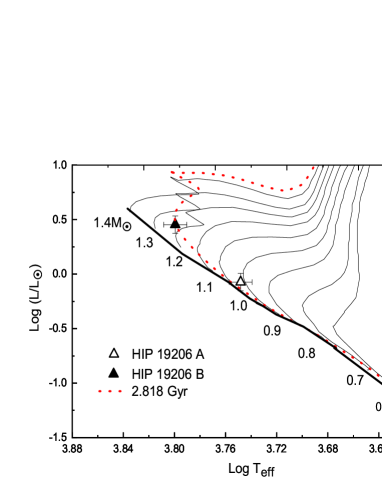
(a) HIP 19206

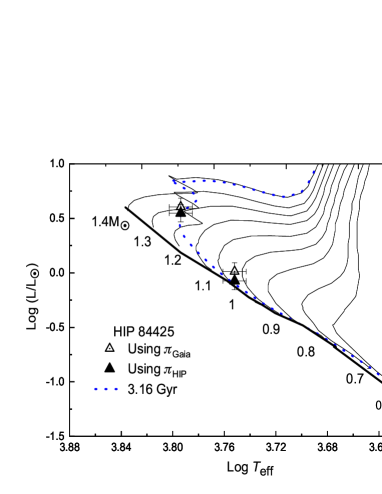
(b) HIP 84425

Figure 4: The positions of the components of HIP 19206 and HIP 84425 on the evolutionary tracks of [Girardi et al.(2000)] for the masses ( 0.6, 0.7, …., 1.4 $\rm\,M_{\odot}$). Figure b shows the positions of the components as been estimated using the parallaxes given by Hipparcos and Gaia (See Table 1).

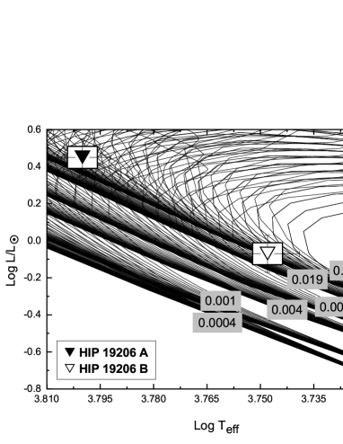
(a) HIP 19206

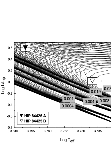
(b) HIP 84425

Figure 5: The positions of the components of HIP 19206 and HIP 84425 on the isochrones of low- and intermediate-mass stars of different metallicities. The isochrones were taken from [Girardi et al.(2000)].

6 Conclusions

Using the recent parallax measurements given by Gaia (Gaia DR2), we were able to present a complete analysis for the two CVBSs HIP 19206 and HIP 84425.

The technique uses a dynamical and a spectrophotometrical methods in a complementary iterated way, to estimate the complete set of their fundamental parameters.

In order to get the precise fundamental parameters of the systems, We used a combination of a dynamical method (ORBITX) [Tokovinin et al.(2016)], and a computational spectrophotometrical method (Al-Wardat’s method for analyzing CVBMSs as , which employs grids of [Kurucz(1994)] line-blanketed plane-parallel model atmospheres (ATLAS 9) for single stars).

As well known in astrophysics, masses of the BSs’ components represent one of the crucial parameters, either for being a common parameter between the dynamical method and the spectrophotometrical one, or for being one of the most important results of the analysis for their essential role in stellar evolution theories.

The analysis of the the systems under study showed a good consistency between the mass sum using the dynamical solutions and the masses estimated using Al-Wardat’s method. But, in order to achieve a better consistency, a new dynamical parallax is given in this work for both systems.

The results show that the components of HIP 19206 system are main sequence stars, and the components of Hip 84425 have left the main sequence to the sub-giant stage. The components of each system have almost similar parameters and same age. Hence, fragmentation is the most probable process for the formation and evolution of both systems, where [Bonnell(1994)] concluded that fragmentation of rotating disk around an incipient central protostar is possible, as long as there is continuing in fall, and [Zinnecker & Mathieu(2001)] pointed out that hierarchical fragmentation during rotational collapse has been invoked to produce binaries and multiple systems.

As consequence, the results of such studies would improve our understanding of the nature, formation and evolution of binary and multiple stellar systems.

Finally, synthetic photometry, consistency of the results between the two methods and consistency between some parameters with the available observational data give an indication about the accuracy of the used methods, and hence the estimated stellar parameters for both systems.

7 ACKNOWLEDGMENTS

The data that support the findings of this study are openly available in The Gaia Data Release 2 (Gaia DR2 ) at https://gea.esac.esa.int/archive. This research has made use of SAO/NASA, SIMBAD database, Fourth Catalog of Interferometric Measurements of Binary Stars, Sixth Catalog of Orbits of Visual Binary Stars, IPAC data systems, ORBITX code and Al-Wardat’s complex method for analyzing close visual binary and multiple systems with its codes.

References

- [Al-Wardat(2002)] Al-Wardat, M. A. 2002, Bulletin of the Special Astrophysics Observatory, 53, 51
- [Al-Wardat(2007)] Al-Wardat, M. A. 2007, Astronomische Nachrichten, 328, 63
- [Al-Wardat(2009)] Al-Wardat, M. A. 2009, Astronomische Nachrichten, 330, 385
- [Al-Wardat(2012)] Al-Wardat, M. A. 2012, PASA, 29, 523
- [Al-Wardat(2014)] Al-Wardat, M. A. 2014, Astrophysical Bulletin, 69, 454
- [Al-Wardat et al.(2014a)] Al-Wardat, M. A., Balega, Y. Y., Leushin, V. V., et al. 2014a, Astrophysical Bulletin, 69, 58
- [Al-Wardat et al.(2016)] Al-Wardat, M. A., El-Mahameed, M. H., Yusuf, N. A., Khasawneh, A. M., & Masda, S. G. 2016, Research in Astronomy and Astrophysics, 16, 166
- [Al-Wardat et al.(2021)] Al-Wardat, M. A., Hussein, A. M., Al-Naimiy, H. M., & Barstow, M. A. 2021, Publications of the Astronomical Society of Australia, 38, e002
- [Al-Wardat et al.(2014b)] Al-Wardat, M. A., Widyan, H. S., & Al-thyabat, A. 2014b, PASA, 31, e005
- [Al-Wardat et al.(2017)] Al-Wardat, M., Docobo, J., Abushattal, A., & Campo, P. 2017, Astrophysical Bulletin, 72, 24
- [Balega et al.(2006a)] Balega, I. I., Balega, A. F., Maksimov, E. V., et al. 2006a, Bull. Special Astrophys. Obs., 59, 20
- [Balega et al.(2006b)] Balega, I. I., Balega, Y. Y., Hofmann, K.-H., et al. 2006b, A&A, 448, 703
- [Balega et al.(2007)] Balega, I. I., Balega, Y. Y., Maksimov, A. F., et al. 2007, Astrophysical Bulletin, 62, 339
- [Bonnell(1994)] Bonnell, I. A. 1994, in Astronomical Society of the Pacific Conference Series, Vol. 65, Clouds, Cores, and Low Mass Stars, ed. D. P. Clemens & R. Barvainis, 115
- [Brown et al.(2020)] Brown, A. G., Vallenari, A., Prusti, T., et al. 2020, arXiv preprint arXiv:2012.01533
- [Collaboration et al.(2018)] Collaboration, G., et al. 2018, VizieR Online Data Catalog, 1345
- [ESA(1997)] ESA. 1997, The Hipparcos and Tycho Catalogues (ESA)
- [Girardi et al.(2000)] Girardi, L., Bressan, A., Bertelli, G., & Chiosi, C. 2000, A&AS, 141, 371
- [Girardi et al.(2000)] Girardi, L., Bressan, A., Bertelli, G., & Chiosi, C. 2000, Astronomy and Astrophysics Supplement Series, 141, 371
- [Girardi et al.(2000)] Girardi, L., Bressan, A., Bertelli, G., & Chiosi, C. 2000, VizieR Online Data Catalog, 414, 10371
- [Gray(2005)] Gray, D. F. 2005, The Observation and Analysis of Stellar Photospheres, 505
- [Hartkopf et al.(2001)] Hartkopf, W. I., McAlister, H. A., & Mason, B. D. 2001, AJ, 122, 3480
- [Horch et al.(2008)] Horch, E. P., van Altena, W. F., Cyr, William M., J., et al. 2008, AJ, 136, 312
- [Kurucz(1994)] Kurucz, R. 1994, Solar abundance model atmospheres for 0,1,2,4,8 km/s. Kurucz CD-ROM No. 19. Cambridge, Mass.: Smithsonian Astrophysical Observatory, 1994., 19
- [Lallement et al.(2018)] Lallement, R., Capitanio, L., Ruiz-Dern, L., et al. 2018, A&A, 616, A132
- [Lang(1992)] Lang, K. 1992, Astrophysical Data: Planets and Stars, 132ff
- [Lang(1992)] Lang, K. R. 1992, Astrophysical Data I. Planets and Stars., 133
- [Maíz Apellániz(2007)] Maíz Apellániz, J. 2007, in Astronomical Society of the Pacific Conference Series, Vol. 364, The Future of Photometric, Spectrophotometric and Polarimetric Standardization, ed. C. Sterken (San Francisco: Astronomical Society of the Pacific), 227
- [Masda et al.(2019)] Masda, S., Docobo, J., Hussein, A., et al. 2019, Astrophysical Bulletin, 74, 464
- [Masda et al.(2016)] Masda, S. G., Al-Wardat, M. A., Neuhäuser, R., & Al-Naimiy, H. M. 2016, Research in Astronomy and Astrophysics, 16, 112
- [Masda et al.(2019)] Masda, S. G., Docobo, J. A., Hussein, A. M., et al. 2019, Astrophysical Bulletin, 74, 464
- [Mason et al.(2018)] Mason, B. D., Hartkopf, W. I., Miles, K. N., et al. 2018, VizieR Online Data Catalog, J/AJ/155/215
- [Rica Romero(2010)] Rica Romero, F. M. 2010, Revista Mexicana de Astronomía y Astrofísica, 46, 263
- [Shatskii & Tokovinin(1998)] Shatskii, N. I., & Tokovinin, A. A. 1998, Astronomy Letters, 24, 673
- [Söderhjelm(1999)] Söderhjelm, S. 1999, Astronomy and Astrophysics, 341, 121
- [Tokovinin(2019)] Tokovinin, A. 2019, IAU Commission on Double Stars, 199, 2
- [Tokovinin et al.(2010)] Tokovinin, A., Mason, B. D., & Hartkopf, W. I. 2010, AJ, 139, 743
- [Tokovinin et al.(2015)] Tokovinin, A., Mason, B. D., Hartkopf, W. I., Mendez, R. A., & Horch, E. P. 2015, AJ, 150, 50
- [Tokovinin et al.(2016)] Tokovinin, A., Mason, B. D., Hartkopf, W. I., Mendez, R. A., & Horch, E. P. 2016, AJ, 151, 153
- [van Leeuwen(2007)] van Leeuwen, F. 2007, A&A, 474, 653
- [Zinnecker & Mathieu(2001)] Zinnecker, H., & Mathieu, R., eds. 2001, IAU Symposium, Vol. 200, The Formation of Binary Stars