Episodic Multi-Agent Reinforcement Learning with Curiosity-Driven Exploration

Abstract

Efficient exploration in deep cooperative multi-agent reinforcement learning (MARL) still remains challenging in complex coordination problems. In this paper, we introduce a novel Episodic Multi-agent reinforcement learning with Curiosity-driven exploration algorithm, named EMC. EMC uses prediction errors of individual Q-value functions as intrinsic rewards for coordinated exploration and leverages episodic memory to exploit explored informative experience to boost policy training. As the dynamics of an agent’s individual Q-value function captures the novelty of states and the influence from other agents, our intrinsic reward can induce coordinated exploration to new or promising states. We illustrate the advantages of our method by didactic examples, and demonstrate its significant outperformance over state-of-the-art MARL baselines on difficult tasks in StarCraft II micromanagement benchmark.

1 Introduction

Cooperative multi-agent reinforcement learning (MARL) has great promise to solve many real-world multi-agent problems, such as autonomous cars (car) and robots (robot). These complex applications post two major challenges for cooperative MARL: scalability, i.e., the joint-action space exponentially grows as the number of agents increases, and partial observability, which requires agents to make decentralized decisions based on their local action-observation histories due to communication constraints. Luckily, a popular MARL paradigm, called centralized training with decentralized execution (CTDE) (CTDE2002), is adopted to deal with these challenges. With this paradigm, agents’ policies are trained with access to global information in a centralized way and executed only based on local histories in a decentralized way. Based on the paradigm of CTDE, many deep MARL methods have been proposed, including VDN (VDN), QMIX (QMIX), QTRAN (QTRAN), and QPLEX (qplex).

A core idea of these approaches is to use value factorization, which uses neural networks to represent the joint state-action value as a function of individual utility functions, which can be referred to individial Q-values for terminological simplicity. For example, VDN learns a centralized but factorizable joint value function $Q_{tot}$ represented as the summation of individual value function $Q_{i}$. During execution, the decentralized policies can be easily derived for each agent $i$ by greedily selecting actions with respect to its local value function $Q_{i}$. By utilizing this factorization structure, an implicit multi-agent credit assignment is realized because $Q_{i}$ is represented as a latent embedding and is learned by neural network backpropagation from the total temporal-difference error on the single global reward signal, rather than on a local reward signal specific to agent $i$. This value factorization technique enables value-based MARL approaches, such as QMIX and QPLEX, to achieve state-of-the-art performance in challenging tasks such as the StarCraft unit micromanagement (SMAC).

Despite the current success, since only using simple $\epsilon$-greedy exploration strategy, these deep MARL approaches are found ineffective to solve complex coordination tasks that require coordinated and efficient exploration (qplex). Exploration has been extensively studied in single-agent reinforcement learning and many advanced methods have been proposed, including pseudo-counts (COUNT; ostrovski2017count), curiosity (ICM; RND), and information gain (VIME). However, these methods cannot be adopted into MARL directly, due to the exponentially growing state space and partial observability, leaving multi-agent exploration challenging. Recently, only a few works have tried to address this problem. For instance, EDTI (EDTI) uses influence-based methods to quantify the value of agents’ interactions and coordinate exploration towards high-value interactions. This approach empirically shows promising results but, because of the need to explicitly estimate the influence among agents, it is not scalable when the number of agents increases. Another method, called MAVEN (MAVEN), introduces a hierarchical control method with a shared latent variable encouraging committed, temporally extended exploration. However, since the latent variable still needs to explore in the space of joint behaviours (MAVEN), it is not efficient in complex tasks with large state spaces.

In this paper, we propose a novel multi-agent curiosity-driven exploration method. Curiosity is a type of intrinsic motivation for exploration, which usually uses prediction errors on different spaces (e.g., future observations (RND), actions (ICM), or learnable representation (kim2018emi)) as a reward signal. Recently, curiosity-driven methods have achieved significant success in single-agent reinforcement learning (RND; NGU; Agent57). However, curiosity-driven methods face a critical challenge in MARL: in which space should we define curiosity? The straightforward method is to measure curiosity on the global observation (RND) or joint histories in a centralized way. However, it is inefficient to find structured interaction between agents, which seems too sparse compared with the exponentially growing state space when the number of agents increases. In contrast, if curiosity is defined as the novelty of local observation histories during the decentralized execution, although scalable, it still fails to guide agents to coordinate due to partial observability. Therefore, we find a middle point of centralized curiosity and decentralized curiosity, i.e., utilizing the value factorization of the state-of-the-art multi-agent Q-learning approaches and defining the prediction errors of individual Q-value functions as intrinsic rewards. r0.5 CTDE Framework The significance of this intrinsic reward is two-fold: 1) it provides a novelty measure of joint observation histories with scalability because individual Q-values are latent embeddings (i.e., an effective state abstraction (li2006towards)) of observation histories in factorized multi-agent Q-learning (e.g., VDN or QPLEX); and 2) as shown in Figure 1, it captures the influence from other agents due to the implicit credit assignment from global reward signal during centralized training (LVD), and biases exploration into promising states where strong interdependence may lie between agents. Therefore, with this novel intrinsic reward, our curiosity-driven method enables efficient, diverse, and coordinated exploration for deep multi-agent Q-learning with value factorization.

Besides efficient exploration, another challenge for deep MARL approaches is how to make the best use of experiences collected by the exploration strategy. Prioritized experience replay based on TD errors shows effectiveness in single-agent deep reinforcement learning. However, it does not carry this promise in factorized multi-agent Q-learning, since the projection error induced by value factorization is also fused into the TD error and severally degrades the effectiveness of the TD error as a measure of the usefulness of experiences. To efficiently use promising exploratory experience trajectories, we augment factorized multi-agent reinforcement learning with episodic memory (emdqn; zhu2019episodic). This memory stores and regularly updates the best returns for explored states. We use the results in the episodic memory to regularize the TD loss, which allows fast latching onto past successful experience trajectories collected by curiosity-driven exploration and greatly improves learning efficiency. Therefore, we call our method Episodic Multi-agent reinforcement learning with Curiosity-driven exploration, called EMC.

We evaluate EMC in didactic examples, and a broad set of StarCraft II micromanagement benchmark tasks (SMAC). The didactic examples along with detailed visualization illustrate that our proposed intrinsic reward can guide agents’ policies to novel or promising states, thus enabling effectively coordinated exploration. Empirical results on more complicated StarCraft II tasks show that EMC significantly outperforms other multi-agent state-of-the-art baselines.

2 Background

2.1 Dec-POMDP

A cooperative multi-agent task can be modelled as a Dec-POMDP (Dec-POMDP), which is defined by a tuple $G=<\mathcal{I},\mathcal{S},\mathcal{A},P,R,\Omega,O,n,\gamma>$, where $\mathcal{I}$ is the sets of $n$ agents, $\mathcal{S}$ is the global state space, $\mathcal{A}$ is the finite action set, $\gamma\in[0,1)$ is the discount factor. We consider a partially observable setting in a Dec-POMDP, i.e., at each timestep, agent $i\in\mathcal{I}$ only has access to the observation $o_{i}\in\Omega$ drawn from the observation function $O(s,i)$. Besides, each agent has an action-observation history $\tau_{i}\in{\mathcal{T}}\equiv\left(\Omega\times\mathcal{A}\right)^{*}$ and constructs its individual policy to jointly maximize team performance. With each agent $i$ selecting an action $a_{i}\in\mathcal{A}$, the joint action $\bm{a}\equiv[a_{i}]_{i=1}^{n}\in\bm{\mathcal{A}}\equiv{{\mathcal{A}}^{N}}$ leads to a shared reward $r=R(s,\bm{a})$ and the next state $s^{\prime}$ according to the transition function $P(s^{\prime}|s,\bm{a})$. Denote $\bm{\tau}\in\bm{\mathcal{T}}\equiv\mathcal{T}^{N}$, the formal objective function is to find a joint policy $\bm{\pi}$ that maximizes a joint value function $V^{\bm{\pi}}(s)=\mathbb{E}[\sum_{t=0}^{\infty}\gamma^{t}r_{t}|s=s_{0},\bm{\pi}]$, or a joint action-value function $Q^{\pi}(s,\bm{a})=r(s,\bm{a})+\gamma\mathbb{E}_{s^{\prime}}[V^{\bm{\pi}}(s^{\prime})]$.

2.2 Centralized Training With Decentralized Execution(CTDE)

CTDE is a promising paradigm in deep cooperative multi-agent reinforcement learning(CTDE1; CTDE2), where the local agents execute actions only based on local observation histories, while the policies can be trained in centralized manager which has access to global information. During the training process, the whole team cooperate to find the optimal joint action-value function $Q^{*}(s,\bm{a})=r(s,\bm{a})+\gamma\mathbb{E}_{s^{\prime}}[max_{\bm{a^{\prime}}}Q^{*}(s^{\prime},\bm{a^{\prime}})]$. Due to partial observability, we use $Q(\bm{\tau},\bm{a};\bm{\theta})$ instead of $Q(s,\bm{a};\bm{\theta})$. Then the Q-value nenurl network will be optimized by the following expected TD-error:

$$\mathcal{L(\bm{\theta})}=\mathbb{E}_{\bm{\tau},\bm{a},\bm{r},\bm{\tau^{\prime}}\in D}\left[r+\gamma V(\bm{\tau^{\prime}};\bm{\theta}^{-})-Q(s,\bm{a};\bm{\theta})\right]^{2}$$ (1)

where $D$ is the replay buffer and $\bm{\theta}^{-}$ denotes the parameters of the target network, which is periodically updated by $\bm{\theta}$. And $V(\bm{\tau^{\prime}};\bm{\theta}^{-})$ is the one-step expected future return of the TD target. However, local agents can only obtain local action-observation history and need inference based on individual Q-value functions $Q_{i}(\tau_{i},a_{i})$. Therefore, to realize effective value-based CTDE, it is critical that the joint greedy action should be equivalent to the collection of individual greedy actions of local agents, which is called IGM (Individual-Global-Max) (QTRAN): $\forall{\bm{\tau}}\in\bm{\mathcal{T}}$,

$$\operatorname*{arg\,max}_{\bm{a}\in\bm{\mathcal{A}}}Q_{tot}(\bm{\tau},\bm{a})=$$ (2)

$$\left(\operatorname*{arg\,max}_{a_{1}\in\mathcal{A}}Q_{1}(\tau_{1},a_{1}),\cdots,\operatorname*{arg\,max}_{a_{n}\in\mathcal{A}}Q_{n}(\tau_{n},a_{n})\right),$$

where $Q_{tot}$ stands for the joint Q-value function. Many works have made efforts in finding the factorization structures between joint Q-value functions and individual Q-functions(QMIX; qplex; VDN) and attracted great attention.

2.3 Episodic Control

Episodic Control is used in near-deterministic reinforcement learning to improve sample efficiency (lengyel2008hippocampal; MFEC; emdqn; pritzel2017neural; hansen2018fast; zhu2019episodic). Since the reward propagation is slow in Q-learning as only provides updates of one-step reward or close-by multi-step rewards (TD($\lambda$)), episodic reinforcement learning is studied broadly to speed up the learning process by a non-parametric episodic memory in single-agent setting. The key idea of episodic control is to store good past experiences in a tabular-based non-parametric memory. When encountering similar states, the agent can rapidly latch onto past successful polices thus boost training, instead of waiting for many steps of optimization. For example, model-free episodic control method (MFEC) records the the maximum return among all these rollouts starting from the intersection $(s,a)$, i.e.,

$$Q^{EC}(s_{t},a_{t})=\begin{cases}R_{t}\quad\quad\quad\quad\quad\quad\quad\text{if}(s_{t},a_{t})\notin Q^{EC},\\ \max{\left(R_{t},Q^{EC}(s_{t},a_{t})\right)}\quad\text{otherwise,}\end{cases}$$ (3)

When execution, MFEC references Episodic Memory table and selects the action with the max Q value of the current state. If lacking exact match in current memory table, MFEC will try to find the k-nearest-neighbors performs of the key state and estimate the state-action values, i.e.,

$$\hat{Q}^{EC}(s,a)=\left\{\begin{aligned} &\frac{1}{k}\sum_{i=1}^{k}Q(s_{i},a)&\mbox{if }(s_{t},a_{t})\notin Q^{EC},\\ &Q^{EC}(s,a)&\mbox{otherwise,}\\ \end{aligned}\right.$$ (4)

where $s_{i},i=1,\cdots,k$ are the $k$ nearest states from $s$. In practice, some method uses exact match instead of KNN for time-efficient querying.

3 Episodic Multi-agent Reinforcement Learning with Curiosity-Driven Exploration

In this section, we introduce EMC, a novel episodic multi-agent exploration framework. EMC takes prediction errors of individual Q-value functions as intrinsic rewards for guiding the diverse and coordinated exploration. After collecting informative experience, we leverage an episodic memory to memorize the highly rewarding sequences and use it as the reference of a one-step TD target to boost multi-agent Q-learning. First, we analyze the motivations for predicting individual Q-values, then we introduce the curiosity module for exploration. Finally, we describe how to utilize episodic memory to boost training.

3.1 Curiosity-Driven Exploration by Predicting Individual Q-values

As shown in Figure 1, in the paradigm of CDTE, local agents make decisions based on individual Q-value functions, which take local observation histories as inputs, and are updated by the centralized module which has access to global information for training. The key insight is that, different from single-agent cases, individual Q-value functions in MARL are used for both decision-making and embedding historical observations. Furthermore, due to implicit credit assignment by global reward signal during centralized training, individual Q-value functions $Q_{i}(\tau_{i},\cdot)$ are influenced by environment as well as other agents’ behaviors. More concretely, it has been proved by Wang et al. (LVD) that, when the joint Q-function $Q_{tot}$ is factorized into linear combination of individual Q-functions $Q_{i}$, i.e., $Q_{tot}^{(t+1)}(\bm{\tau},\bm{a})=\sum_{i=1}^{N}Q_{i}^{(t+1)}(\tau_{i},a_{i})$, then $Q_{i}^{(t+1)}(\tau_{i},a_{i})$ has the following closed-form solution:

$$Q_{i}^{(t+1)}(\tau_{i},a_{i})= \underbrace{\mathop{\mathbb{E}}_{(\tau^{\prime}_{-i},a^{\prime}_{-i})\sim p_{D}(\cdot|{\tau_{i}})}\left[y^{(t)}\left(\tau_{i}\oplus\tau^{\prime}_{-i},a_{i}\oplus a^{\prime}_{-i}\right)\right]}_{\text{evaluation of the individual action $a_{i}$}}$$ (5)

$$-\frac{n-1}{n}\underbrace{\mathop{\mathbb{E}}_{{\bm{\tau}}^{\prime},\bm{a}^{\prime}\sim p_{D}(\cdot|\Lambda^{-1}({\tau_{i}}))}\left[y^{(t)}\left({\bm{\tau}}^{\prime},\bm{a}^{\prime}\right)\right]}_{\text{counterfactual baseline}}+w_{i}(\tau_{i}),$$

where $y^{(t)}({\bm{\tau}},\bm{a})=r+\gamma\mathbb{E}_{{\bm{\tau}}^{\prime}}\left[\max_{\bm{a}^{\prime}}Q^{(t)}_{tot}\left({\bm{\tau}}^{\prime},\bm{a}^{\prime}\right)\right]$ denotes the expected one-step TD target, and $p_{D}(\cdot|\tau_{i})$ denotes the conditional empirical probability of $\tau_{i}$ in the given dataset $D$. The notation $\tau_{i}\oplus\tau^{\prime}_{-i}$ denotes $\langle\tau_{1}^{\prime},\dots,\tau_{i-1}^{\prime},\tau_{i},\tau_{i+1}^{\prime},\dots,\tau_{n}^{\prime}\rangle$, and $\tau^{\prime}_{-i}$ denotes the elements of all agents except for agent $i$. $\Lambda^{-1}(\tau_{i})$ denotes the set of trajectory histories that may share the same latent-state trajectory as $\tau_{i}$. The residue term $\bm{w}\equiv\left[w_{i}\right]_{i=1}^{n}$ is an arbitrary function satisfying $\forall\bm{\tau}\in\bm{\Gamma}$, $\sum_{i=1}^{n}w_{i}(\tau_{i})=0$.

Eq. (5) shows that by linear value factorization, the individual Q-value $Q_{i}(\tau_{i},a_{i})$ is not only decided by local observation histories but also influenced by other agents’ action-observation histories. Thus predicting $Q_{i}$ can capture both the novelty of states and the interaction between agents and lead agents to explore promising states. Motivated by this insight, in this paper, we use a linear value factorization module separate from the inference module to learn the individual value function $Q_{i}$, and use the prediction errors of $Q_{i}$ as intrinsic rewards to guide exploration. In this paper, we define the prediction errors of individual Q-values as curiosity and propose our curiosity-driven exploration module as follows.

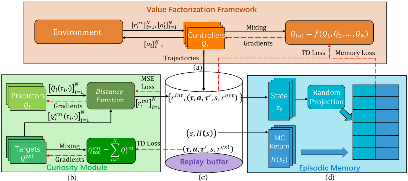
Figure 1: An overview of EMC’s framework

Figure 1b demonstrates the Curiosity Module, separated from the inference module (Figure 1a). The curiosity module consists of four components: (i) The centralized training part with linear value factorization, which shares the same implementation as VDN (VDN), but only trained with extrinsic rewards $r^{ext}$ from the environment; (ii) the Target for prediction, i.e., the corresponding individual Q-values $Q_{i}^{ext}$, represented by a recurrent Q-network; (iii) Predictor $\widetilde{Q}_{i}(\tau_{i})$, which is used for predicting $Q_{i}^{ext}$ and shares the same network architecture as Target $Q_{i}^{ext}$; and (iv) Distance Function, which measures the distance between $Q_{i}^{ext}$ and $\widetilde{Q}_{i}$, e.g., $L_{2}$ distance. The predictors are trained by minimizing the Mean Squared Error (MSE) of the distance in an end-to-end manner. For stable training, we use the soft-update target (softupdate) of $Q_{i}^{ext}$ to smooth the outputs of the targets. In general, (ii) is trained with (i) and outputs individual Q-values , while (iii) is trained with (ii) and (iv), and aims to predict the soft-update target of individual Q-values. Motivated by the implicit credit assignment of linear value factorization (Eq. (5)), the curiosity module predicts the individual Q-values $\left[Q^{ext}_{i}\right]_{i=1}^{n}$ in linear factorization, i.e., $Q^{ext}_{tot}=\sum_{i=1}^{N}Q_{i}^{ext}$. Then the curiosity-driven intrinsic reward is generated by the following equation:

$$r^{int}=\frac{1}{N}\sum_{i=1}^{N}{\left\|\widetilde{Q}_{i}(\tau_{i},\cdot)-{Q}^{ext}_{i}(\tau_{i},\cdot)\right\|}_{2}\\ ,$$ (6)

This intrinsic reward is used for the centralized training of the inference module, as shown in Figure 1a:

$$\mathcal{L_{\text{inference}}(\bm{\theta})}=\mathbb{E}_{\bm{\tau},\bm{a},\bm{r},\bm{\tau}^{\prime}\in D}\left[\left(y(\bm{\tau},\bm{a})-Q_{tot}(\bm{\tau},\bm{a};\bm{\theta})\right)^{2}\right],$$ (7)

where $y(\bm{\tau},\bm{a})=r^{ext}+\beta r^{int}+\gamma\max_{\bm{a}^{\prime}}Q_{tot}\left({\bm{\tau}}^{\prime},\bm{a}^{\prime};\bm{\theta}^{-})\right)$, denoting one step TD target of the inference module, and $\beta$ is the weight term of the intrinsic reward. We use a separate training model for inference (Figure 1a) to avoid the accumulation of projection errors of $Q_{i}$ during training.

The independence of inference module leads to another advantage, that EMC’s architecture can be adopted into many value-factorization-based multi-agent algorithms which utilize the CDTE paradigm, i.e., the general function $f$ in Figure 1a can indicate specific (linear, monotonic and IGM) value factorization structures in VDN (VDN), QMIX (QMIX), and QPLEX (qplex), respectively. In this paper, we utilize these state-of-the-art algorithms for the inference module. With this curiosity-driven bias plugged into ordinary MARL algorithms, EMC will achieve efficient, diverse and coordinated exploration.

3.2 Episodic Memory

Equipped with efficient exploration ability, another challenge is how to make the best use of good trajectories collected by exploration effectively. Recently, episodic control has been widely studied in single-agent reinforcement learning (emdqn; zhu2019episodic), which can replay the highly rewarding sequences, thus boosting training. Inspired by this framework, we generalize single-agent episodic control to propose a multi-agent episodic memory, which records the best memorized Monte-Carlo return in the episode, and provide a memory target $H$ as a reference to regularize the ordinary one-step inference TD target estimation in the inference module (Figure 1a):

$$\mathcal{L_{\text{memory}}(\bm{\theta})}=\mathbb{E}_{\bm{\tau},\bm{a},\bm{r},\bm{\tau}^{\prime}\in D}\left[\left(H-Q_{tot}(\bm{\tau},\bm{a};\bm{\theta})\right)^{2}\right].$$ (8)

However, different from the single-agent episodic control, the action space of MARL exponentially grows as the number of agents increases, and partial observability also limits the information of individual value functions. Thus, we maintain our episodic memory by storing the state-value function on the global state space and utilizing the global information during the centralized training process under the CTDE paradigm. Figure 1d shows the architecture of the Episodic Memory. We keep a memory table $M$ to record the maximum remembered return of the current state, and use a fixed random matrix drawn from Gaussian distribution as a representation function to project states into low-dimensional vectors $\phi(s):S\rightarrow{\mathbb{R}^{k}}$, which are used as keys to look up corresponding global state value function $H(\phi(s_{t}))$. When our exploration method collects a new trajectory, we update our memory table $M$ as follows:

$$H(\phi(s_{t}))=\begin{cases}\max\{H(\phi(\hat{s}_{t})),R_{t}(s_{t},\bm{a}_{t})\}&{\textit{if }\|\phi(\hat{s}_{t})-\phi(s_{t})\|_{2}<\delta}\\ R_{t}(s_{t},\bm{a}_{t})&otherwise\end{cases},$$ (9)

where $\phi(\hat{s}_{t})$ is $\phi(s_{t})$’s nearest neighbor in the memory $M$, $\delta$ is a threshold, and $R(s_{t},\bm{a}_{t})$ represents the future return when agents taking joint action $\bm{a}_{t}$ under global state $s_{t}$ at the $t$-th timestep in a new episode. In our implementation, $\phi(s_{t})\in M$ is indeed evaluated approximately based on the embedding distance. Specifically, when the key of the state $\phi(s_{t})$ is close enough to one key in the memory, we assume that $\phi(s_{t})\in M$ and find the best memorized Monte-Carlo return correspondingly. Otherwise, we think $\phi(s_{t})\notin M$ and record the state’s return into the memory. Leveraging the episodic memory, we can directly obtain the maximum remembered return of the current state, and use the one-step TD memory target $H$ as a reference to regularize learning:

$${H}(\phi(s_{t}),\bm{a}_{t})=r_{t}(s_{t},\bm{a}_{t})+\gamma H(\phi(s_{t+1})).$$ (10)

Thus, the new objective function for the inference module is:

$$\mathcal{L_{\text{total}}(\bm{\theta})} =\mathcal{L_{\text{inference}}(\bm{\theta})}+\lambda\mathcal{L_{\text{memory}}(\bm{\theta})}$$ (11)

$$=\mathbb{E}_{\bm{\tau},\bm{a},\bm{r},\bm{\tau}^{\prime}\in D}\left[\left(y(\bm{\tau},\bm{a})-Q_{tot}(\bm{\tau},\bm{a};\bm{\theta})\right)^{2}+\lambda\left(H\left(\phi(s_{t}),\bm{a}_{t}\right)-Q_{tot}(\bm{\tau},\bm{a};\bm{\theta})\right)^{2}\right],$$

where $\lambda$ is the weighting term to balance the effect of episodic memory’s reference. Using the maximum return from the episodic memory to propagate rewards, we can compensate for the disadvantage of slow learning induced by the original one-step reward update and improve sample efficiency.

4 Experiments

In this section we will analyse experiments results designed for answering following questions: (1) Is predicting individual Q-value functions better than predicting the history of observations?  (Section 4.1)(2) Can our method perform well due to the improved coordination exploration in challenging multi-agent tasks? (Section 4.2) (3) if so, what role does each key component play in the outperformance? (Section 4.3) We propose a didactic example and demonstrate the advantage of our method in coordinated exploration, and evaluate our method in the StarCraft II micromanagement (SMAC) benchmark (SMAC) compared with existing state-of-the-art multi-agent reinforcement learning (MARL) algorithms: QPLEX (qplex), Weighted-QMIX(weightedqmix), RODE(wang2020rode), and multi-agent exploration method MAVEN(MAVEN).

4.1 Didactic Example

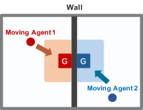
(a) Coordinated Toygame

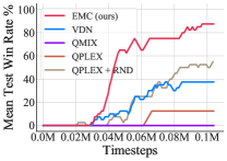
(b) Performance

Figure 2: Didactic Example

(a) corridor

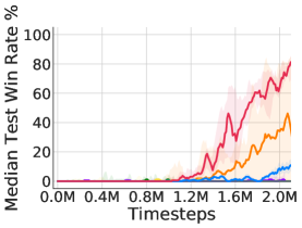
(b) 3s5z_vs_3s6z

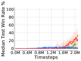
(c) 6h_vs_8z

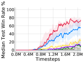
(d) 1c3s8z_vs_1c3s9z

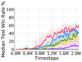
(e) 5s10z

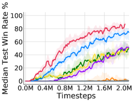
(f) 7s7z

Figure 3: Results of the maps where our method significantly outperforms the other algorithms in the SMAC experiments. The three maps in the second row are draw from QPLEX

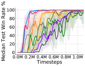
(a) 2s_vs_1sc

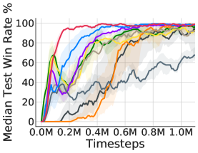
(b) 2s3z

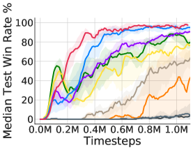
(c) 3s5z

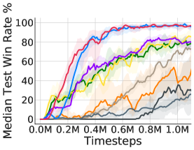
(d) 1c3s5z

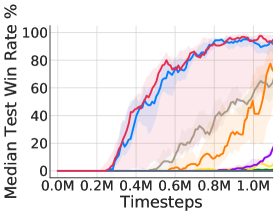
(e) 3s_vs_5z

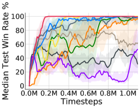
(f) bane_vs_bane

Figure 4: Results of the $6$ easy maps in the SMAC experiments

Figure 2(a) shows another grid world game setting which needs coordinated exploration. The blue agent and red agent can choose one of the five actions: [up, down, left, right, stay] at each time step. The two agents is isolated by the wall, and they cannot be observed by the other one until they get into the light shaded area. Agents explore by using (a) $\epsilon$-greedy strategy, or (b) $\epsilon$-greedy strategy along with intrinsic reward via individual Q-value predictions. They will receive a global positive reward if and only if they arrive at the dark shaded grid at the same time. If only one arrives, the incoordination will be punished by a negative reward. To evaluate the coordinated exploration ability of our method, we test our method in this toygame compared with the following baselines: VDN(VDN), QMIX(QMIX), QPLEX with RND(RND), QPLEX(qplex). Figure 2 shows the average test win rate of these methods over $8$ random seeds and Our method has significantly outperformed other baselines.

To understand this result better, we have made several visualisations to demonstrate our advantage in coordinated exploration. From Figure 6 in Appendix, due to a larger variance of individual Q-value functions caused by the influence between other agents, the two agents will explore in light shaded area more often than other area, thus has higher visiting frequency in this area. Besides, in Figure 7 in Appendix, we can conclude that more successful trajectories can be founded in the replay buffer by our method than QPLEX with RND. The two pictures show that predicting observations will induce a more uniform coverage area, thus may be too inefficient to handle complex tasks when the state space is exponentially large or coordinated exploration need to be addressed. Since predicting Q-value functions can induce coordinated exploration into new or promising states, our method outperforms other method in terms of coordinated exploration.

4.2 StarCraftII Micromanagement (SMAC) Benchmark

For investigating our EMC algorithm would perform in more complex multi-agent environments, we conduct experiments in 17 benchmark tasks of StarCraft II, which contains 14 popular tasks proposed by SMAC (SMAC), and three super hard cooperative tasks proposed by QPLEX (qplex). In the micromanagement scenarios, each unit is controlled by an independent agent that must act based on its own local observation and needs to maximize the damage to enemy units while minimizing damage received. Rewards provided to agents are based on the hitpoint damage dealt and enemy units killed, together with a special bonus for winning the battle. Among the 17 tasks, the corridor, 3s5z_vs_3s6z, 2c_vs_64zg,5s10z,1c3s8z_vs_1c3s9z, 7s7z,6h_vs_8z, 27m_vs_30m, and MMM2 tasks are very difficult for the state-of-the-art MARL algorithms and efficient exploration is one of the important keys to solving these tasks. For the other tasks, exploration may not be that important, but stable learning and efficient coordination are still required.

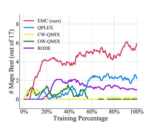
Figure 5: The overall performance of the algorithms in the SMAC experiments. The y-axis is the number of scenarios (out of 17 scenarios) in which the algorithm’s median test win rate is the highest by as least 1/32, and the x-axis is the progress rate of training

Baseline Methods: We compare the EMC algorithm with the baseline algorithms RODE (wang2020rode), QPLEX (qplex), MAVEN (MAVEN), and the two variants CW-QMIX and OW-QMIX (WQMIX) of QMIX (QMIX). It should be noted that MAVEN is designed for multi-agent exploration, while the other baseline algorithms are the state-of-the-art MARL algorithms without special exploration mechanisms. We only test the MAVEN algorithm in the $6$ maps which needs exploration. In the other maps, MAVEN has no advantage than the other algorithms.

Training Settings: All the tested algorithms are trained for $1$ million steps in easy maps such as 2s_vs_1sc, and are trained for $2$ million steps in hard maps such as corridor. Each algorithm is trained using $5$ random seeds and the corresponding results are averaged over the $5$ tests. The baseline algorithms use the $\epsilon$-greedy method for exploration, with the exploration factor $\epsilon$ decaying linearly from $1.0$ to $0.05$ in $50$k steps. During the training process of each algorithm, we conduct evaluation for $32$ episodes every $10$k time steps and record the win rate of the algorithm in the $32$ episodes. The other settings and the implementation details of each algorithm can be found in Appendix.

Results: All experimental results are illustrated with the median performance and 25-75% percentiles. For better comparison and illustration, we plot the results in three figures. Figure 5 shows the overall performance of the tested algorithms in all these $17$ maps. Figure 4 shows the performance of all tested algorithm in $6$ easy maps 2s_vs_1sc, 2s3z, 3s5z, 1c3s5z, 3s_vs_5z, and bane_vs_bane. Figure 3 shows the results of the hard maps where our EMC algorithm performs the best, including corridor, 3s5z_vs_3s6z, 6h_vs_8z, 1c3s8z_vs_1c3s9z, 5s10z, and 7s7z. Due to space limitation, the results of the other maps are plotted in Appendix.

As shown in Figure 5, the EMC algorithm has significantly better performance than the baseline algorithms. The x-axis of the figure is the progress of training and the y-axis represents the number of scenarios (out of 17) where the median win rate of an algorithm is the highest among all algorithms. According to this overall performance measurement, the EMC algorithm remains the best during more than $90\%$ percentage of the training process. At the end of the training process, we can find that EMC performs the best in $6$ out of the $17$ maps, while the second best algorithm only performs best in $2$ out of $17$.

The advantage of our algorithm can be mainly illustrated by the results of the $6$ hard maps shown in Figure 3. Among the $6$ maps, the three maps in the first row are super hard and solving them particularly needs efficient coordinated exploration. Thus, we can find that the EMC algorithm significantly outperforms the other algorithms in corridor and 3s5z_vs_3s6z, and also achieves the best performance (equal to RODE) in 6h_vs_8z. The win rates of EMC appear a very quick boost from time steps $1.2$M and $1.4$M and finally reach about $70\%$ and $90\%$ in Figures 4(a) and 4(b), respectively. To the best of our knowledge, this may be the state-of-the-art results in corridor and 3s5z_vs_3s6z. In contrast, the win rates of the other algorithms (except RODE) in the first three maps remain at a very low level until the end of the $2$M training steps. Interestingly, while the RODE algorithm performs the second best in the first three maps, it fails to learn effective policies and performs the worst in the maps of the second row in Figure 3. For the other algorithms, since the maps 1c3s8z_vs_1c3s9z, 5s10z, and 7s7z are not as difficult as to the first three maps, we can see that their win rates gradually increase during the training process. Due to the boost learning process via episodic memory along with efficient exploration, our algorithm EMC still performs the best in the three maps, with fastest learning speed and the highest rates achieved.

Now examine Figure 4, which corresponds to the $6$ easy maps mentioned above. It can be found that our algorithm perform the best in $5$ of the $6$ easy maps. In the map 2s_vs_1sc, although EMC is the second best, the performance gap between EMC and the QPLEX algorithm is very subtle. The advantage of EMC over the other algorithms can be found in Figures 4(b), 4(c), and 4(f), where it converges much faster than the second best algorithm QPLEX. For example, in the bane_vs_bane tasks, the EMC algorithm reaches a $100\%$ win rate in fewer than $0.2$M steps, while the QPLEX algorithm converges at the time step of $0.3$M. Futhermore, the win rate of QPLEX does not reach $100\%$ in this map and its learning process is not as stable as that of EMC. Therefore, although the state-of-the-art algorithms such as QPLEX performs sufficiently well in these easy maps, the coordinated exploration mechanism and episodic-memory control equipped by EMC can further enhance the performance a learning algorithm.

4.3 Ablation Study

To understand the superior performance of EMC, we carry out ablation studies to test the contribution of its two main components: (1) curiosity module, (2) episodic memory. We test four methods on both the easy and super hard maps. Due to space limitation, here we briefly introduce the main conclusion, and the details of the results are shown in Appendix. The results of the test deliver a message that in easy maps where sufficient exploration can be easily achieved by $\epsilon$-greedy, QPLEX with only the episodic memory module can achieve comparable performance of EMC. However, in the super hard maps, there is a dramatic performance drop if QPLEX only uses episodic memory without curiosity module. It illustrates that the curiosity-driven exploration indeed plays an important role in challenging tasks where coordinated exploration is needed. We test different coefficient $\lambda$ in SC2 tasks and find that a too small $\lambda$ can not boost training, while a larger $\lambda$ will bound the Q-value functions and limit the intrinsic rewards, thus may degenerate performance in super hard tasks.

5 Conclusion

In this paper, we introduce EMC, a novel episodic multi-agent reinforcement learning with curiosity-driven exploration framework that allows efficient coordinated exploration and boosted policy training by exploiting explored informative experience. Based on an effective diverse exploration ability, our method shows significant outperformance over state-of-the-art MARL baselines on difficult tasks in StarCraft II micromanagementbenchmark.