A new proof of Poincaré’s result on the restricted three-body problem

Abstract.

The problem of nonintegrability of the circular restricted three-body problem is very classical and important in dynamical systems. In the first volume of his masterpieces, Henri Poincaré showed the nonexistence of a real-analytic first integral which is functionally independent of the Hamiltonian and real-analytic in a small parameter representing the mass ratio as well as in the state variables, in both the planar and spatial cases. However, his proof was very complicated and unclear. In this paper, we give a new and simple proof of a very similar result for both the planar and spatial cases, using an approach which the author developed recently for nearly integrable systems.

1. Introduction

Figure 1. Configuration of the circular restricted three-body problem in the rotational frame.

In his famous memoir [19], which was related to a prize competition celebrating the 60th birthday of King Oscar II, Henri Poincaré studied the planar circular restricted three-body problem, which is written in the dimensionless form as the Hamiltonian system

$$\begin{split}&\dot{x}=p_{x}+y,\quad\dot{p}_{x}=p_{y}+\frac{\partial U_{2}}{\partial x}(x,y),\\ &\dot{y}=p_{y}-x,\quad\dot{p}_{y}=-p_{x}+\frac{\partial U_{2}}{\partial y}(x,y),\end{split}$$ (1.1)

where

$$U_{2}(x,y)=\frac{\mu}{\sqrt{(x-1+\mu)^{2}+y^{2}}}+\frac{1-\mu}{\sqrt{(x+\mu)^{2}+y^{2}}},$$

and discussed the nonexistence of a real-analytic first integral which is real-analytic in the state variables and parameter $\mu$ near $\mu=0$ and functionally independent of its Hamiltonian

$$H_{2}(x,y,p_{x},p_{y})=\tfrac{1}{2}(p_{x}^{2}+p_{y}^{2})+(p_{x}y-p_{y}x)-U_{2}(x,y).$$

He improved his approach significantly in the first volume of his masterpieces [20] published two years later: he considered not only the planar case (1.1) but also the spatial case

$$\begin{split}&\dot{x}=p_{x}+y,\quad\dot{p}_{x}=p_{y}+\frac{\partial U_{3}}{\partial x}(x,y,z),\\ &\dot{y}=p_{y}-x,\quad\dot{p}_{y}=-p_{x}+\frac{\partial U_{3}}{\partial y}(x,y,z),\\ &\dot{z}=p_{z},\quad\dot{p}_{z}=\frac{\partial U_{3}}{\partial z}(x,y,z),\end{split}$$ (1.2)

where

$$U_{3}(x,y,z)=\frac{\mu}{\sqrt{(x-1+\mu)^{2}+y^{2}+z^{2}}}+\frac{1-\mu}{\sqrt{(x+\mu)^{2}+y^{2}+z^{2}}},$$

and showed the nonexistence of such first integrals. The system (1.2) is also Hamiltonian with the Hamiltonian

$$H_{3}(x,y,z,p_{x},p_{y},p_{z})=\tfrac{1}{2}(p_{x}^{2}+p_{y}^{2}+p_{z}^{2})+(p_{x}y-p_{y}x)-U_{3}(x,y,z)$$

In (1.1) and (1.2), the two primary bodies with mass $\mu$ and $1-\mu$ remain at $(1-\mu,0)$ and $(-\mu,0)$, respectively, on the $xy$-plane in the rotational frame, and the third massless body is subjected to the gravitational forces from them moves under the assumption that the primaries rotate counterclockwise on the circles about their common center of mass at the origin in the inertial coordinate frame (see Fig. 1). See, e.g., Section 4.1 of [13] for more details on the derivation and physical meaning of (1.1) and (1.2). The results of [20] were also explained in [2, 10, 11, 26]. See [4] for an account of his work from mathematical and historical perspectives. His result can be stated as follows.

Theorem 1.1.

The circular restricted three-body problems (1.1) and (1.2) have no real-analytic first integral which is independent of the Hamiltonian and depend real-analytically on $\mu$ near $\mu=0$.

When $\mu=0$, Eqs. (1.1) and (1.2) are integrable and can be transformed to simple Hamiltonian systems in action-angle coordinates (see Eqs. (2.1), (3.9) and (4.7)) by the Delaunay elements (see Eqs. (3.8) and (4.6)). However, in the coordinates, the perturbation terms of $O(\mu)$ are very complicated. Actually, he devoted the whole of Chapter 6, the length of which is 55 pages in the English translated version and 66 pages in the French original one, in [20] to discussions on the perturbation terms. The long and complicated computations are very difficult to understand. Here we prove a result similar to Theorem 1.1 using a different approach which does not rely on the complicated perturbation terms. The planar and spatial cases are discussed in Sections 3 and 4, respectively. See Theorems 3.1 and 4.1 below for the precise statements especially. Our results are more general than Theorem 1.1 in some meaning since it says that the planar and spatial problems (1.1) and (1.2) are not only analytically but also meromorphically nonintegarble. Moreover, they are proven to be nonintegrable even in some resonant planar elliptic orbits. See also Remarks 3.2 and 4.2. However, in another meaning, Theorem 1.1 is more general than ours since it says that they are real-analytically nonintegrable and guarantees no additional first integral in the spatial problem (1.2).

Our basic tool to obtain the result is a technique developed in [28] for determining whether systems of the form

$$\dot{I}=\varepsilon h(I,\theta;\varepsilon),\quad\dot{\theta}=\omega(I)+\varepsilon g(I,\theta;\varepsilon),\quad(I,\theta)\in\mathbb{R}^{\ell}\times\mathbb{T}^{m},$$ (1.3)

are not meromorphically integrable in the Bogoyavlenskij sense [5], which is an extended concept of integrability to non-Hamiltonian systems, such that the first integrals and commutative vector fields, the existence of which are required for their integrability, depend meromorphically on $\varepsilon$ near $\varepsilon=0$, like the result of Poincaré [19, 20] stated above with $\varepsilon=\mu$, where $\ell,m\in\mathbb{N}$, $\varepsilon$ is a small parameter such that $0<|\varepsilon|\ll 1$, and $\omega:\mathbb{R}^{\ell}\to\mathbb{R}^{m}$, $h:\mathbb{R}^{\ell}\times\mathbb{T}^{m}\times\mathbb{R}\to\mathbb{R}^{\ell}$ and $g:\mathbb{R}^{\ell}\times\mathbb{T}^{m}\times\mathbb{R}\to\mathbb{R}^{m}$ are meromorphic in their arguments. The technique is based on generalized versions due to Ayoul and Zung [3] of the Morales-Ramis theory [14, 15] and its extension, the Morales-Ramis-Simó theory [16], and briefly reviewed in a necessary context in Section 2 for the reader’s convenience. The system (1.3) is Hamiltonian if $\ell=m$ as well as $\varepsilon=0$ or

$$\mathrm{D}_{I}h(I,\theta;\varepsilon)\equiv-\mathrm{D}_{\theta}g(I,\theta;\varepsilon),$$

and non-Hamiltonian if not. If a system is integrable in the Bogoyavlenskij sense and has $\ell$ functionally independent first integrals whose level set has a connected compact set, then it is transformed to (1.3) with $\varepsilon=0$ on the connected compact set [5, 32]. Moreover, in [28], it was proven by using the technique that the planar and spatial problems (1.1) and (1.2) are meromorphically nonintegrable near $(x,y)=(-\mu,0),(1-\mu,0)$ and $(x,y,z)=(-\mu,0,0),(1-\mu,0,0)$, respectively, for any $\mu\in(0,1)$. The results of [28] immediately yield statements similar to ours but a region of the phase space in which the nonexistence of additional first integrals is proven is much narrower than ours. See Theorem 3.1 and 4.1 for more details.

In closing this section we give some comments on other recent or relatively recent remarkable progress in related topics. First, the nonintegrability of the general three-body problem is now well understood. Tsygvintsev [21, 22] proved the nonintegrability of the general planar three-body problem near the Lagrangian parabolic orbits in which the three bodies form an equilateral triangle and move along certain parabolas, using the Ziglin method [30]. Boucher and Weil [7] also obtained a similar result, using the Morales-Ramis theory [14, 15] while the case of equal masses was proven a little earlier in [6]. Moreover, Tsygvintsev [23, 24, 25] proved the nonexistence of a single additional first integral near the Lagrangian parabolic orbits when

$$\frac{m_{1}m_{2}+m_{2}m_{3}+m_{3}m_{1}}{(m_{1}+m_{2}+m_{3})^{2}}\notin\{\tfrac{7}{48},\tfrac{5}{16}\},$$

where $m_{j}$ represents the mass of the $j$th body for $j=1,2,3$. Subsequently, Morales-Ruiz and Simon [17] succeeded in removing the three exceptional cases and extended the result to the space of three or more dimensions. Ziglin [31] also proved the nonintegrability of the general three-body problem near a collinear solution in the space of any dimension when two of the three masses, say $m_{1},m_{2}$, are nearly equal but neither $m_{3}/m_{1}$ nor $m_{3}/m_{2}\in\{11/12,1/4,1/24\}$. It should be noted that Ziglin [31] and Morales-Ruiz and Simon [17] also discussed the general $N$-body problem.

Secondly, Guardia et al. [9] considered the planar problem (1.1) and showed the occurrence of transverse intersection between the stable and unstable manifolds of the infinity for any $\mu\in(0,1)$ in a region far from the primaries in which $r=\sqrt{x^{2}+y^{2}}$ and its conjugate momentum are sufficiently large. This implies, e.g., by Theorem 3.10 of [18], the real-analytic nonintetgrabilty of (1.1) as well as the existence of oscillatory motions such that $\limsup_{t\to\infty}r(t)=\infty$ while $\liminf_{t\to\infty}r(t)<\infty$. Similar results were obtained much earlier when $\mu>0$ is sufficiently small in [12] or for any $\mu\in(0,1)$ except for a certain finite number of the values in [27].

2. Basic Tool

Our proofs of the main results are based on the technique developed in [28] for proving the nonintegrability of nearly integrable dynamical systems, as stated in Section 1. In this section we restrict ourselves to Hamiltonian systems, and review the basic tool in the context.

Figure 2. Assumption (A2).

Consider $n$-degree-of-freedom Hamiltonian systems of the form

$$\dot{I}=-\varepsilon\mathrm{D}_{\theta}\tilde{H}(I,\theta;\varepsilon),\quad\dot{\theta}=\mathrm{D}H_{0}(I)+\varepsilon\mathrm{D}_{I}\tilde{H}(I,\theta;\varepsilon),\quad(I,\theta)\in\mathbb{R}^{n}\times\mathbb{T}^{n},$$ (2.1)

where $n\geq 2$ is an integer, $\varepsilon$ is a small parameter such that $0<|\varepsilon|\ll 1$, and $H_{0}:\mathbb{R}^{n}\to\mathbb{R}$ and $\tilde{H}:\mathbb{R}^{n}\times\mathbb{T}^{n}\times\mathbb{R}\to\mathbb{R}$ are meromorphic in the arguments. The Hamiltonian for (2.1) is given by $H_{0}(I)+\varepsilon\tilde{H}(I,\theta)$. We extend the domain of the independent variable $t$ to a domain including $\mathbb{R}$ in $\mathbb{C}$ and do so for the dependent variables. When $\varepsilon=0$, Eq. (2.1) becomes

$$\dot{I}=0,\quad\dot{\theta}=\omega(I),$$ (2.2)

where $\omega(I)=\mathrm{D}H_{0}(I)$. We assume the following on the unperturbed system (2.2):

1. For some $I^{\ast}\in\mathbb{R}^{n}$, a resonance of multiplicity $n-1$,

   $$\dim_{\mathbb{Q}}\langle\omega_{1}(I^{\ast}),\ldots,\omega_{n}(I^{\ast})\rangle=1,$$

   occurs with $\omega(I^{\ast})\neq 0$, i.e., there exists a constant $\omega^{\ast}>0$ such that

   $$\frac{\omega(I^{\ast})}{\omega^{\ast}}\in\mathbb{Z}^{n}\setminus\{0\}.$$

   where $\omega_{j}(I)$ is the $j$th element of $\omega(I)$ for $j=1,\ldots,n$.

Note that we can replace $\omega^{\ast}$ with $\omega^{\ast}/k$ for any $k\in\mathbb{N}$. We refer to the $n$-dimensional torus $\mathscr{T}^{\ast}=\{(I^{\ast},\theta)\mid\theta\in\mathbb{T}^{n}\}$ as the resonant torus and to periodic orbits $(I,\theta)=(I^{\ast},\omega(I^{\ast})t+\theta_{0})$, $\theta_{0}\in\mathbb{T}^{n}$, on $\mathscr{T}^{\ast}$ as the resonant periodic orbits. Let $T^{\ast}=2\pi/\omega^{\ast}$. We also make the following assumption.

1. For some $\theta\in\mathbb{T}^{n}$ there exists a closed loop $\gamma_{\theta}$ in a domain including $(0,T^{\ast})\subset\mathbb{R}$ in $\mathbb{C}$ such that $\gamma_{\theta}\cap(i\mathbb{R}\cup(T^{\ast}+i\mathbb{R}))=\emptyset$ and

   $$\mathscr{I}(\theta)=-\mathrm{D}\omega(I^{\ast})\int_{\gamma_{\theta}}\mathrm{D}_{\theta}\tilde{H}(I^{\ast},\omega(I^{\ast})\tau+\theta;0)\mathrm{d}\tau$$ (2.3)

   is not zero. See Fig. 2

Note that the condition $\gamma_{\theta}\cap(i\mathbb{R}\cup(T^{\ast}+i\mathbb{R}))=\emptyset$ is not essential in (A2), since it always holds by replacing $\omega^{\ast}$ with $\omega^{\ast}/k$ for sufficiently large $k\in\mathbb{N}$ if necessary. We can prove the following theorem which guarantees that conditions (A1) and (A2) is sufficient for nonintegrability of (2.1) in a certain meaning.

Theorem 2.1.

Let $\Gamma$ be any domain in $\mathbb{C}/T^{\ast}\mathbb{Z}$ containing $\mathbb{R}/T^{\ast}\mathbb{Z}$ and $\gamma_{\theta}$. Suppose that assumption (A1) and (A2) hold for some $\theta=\theta_{0}\in\mathbb{T}^{n}$. Then the system (1.3) is not meromorphically integrable near the resonant periodic orbit $(I,\theta)=(I^{\ast},\omega(I^{\ast})\tau+\theta_{0})$ with $\tau\in\Gamma$ such that the first integrals also depend meromorphically on $\varepsilon$ near $\varepsilon=0$, when the domains of the independent and dependent variables are extended to regions in $\mathbb{C}$ and $\mathbb{C}^{n}\times(\mathbb{C}/2\pi\mathbb{Z})^{n}$, repsectively. Moreover, if (A2) holds for any $\theta\in\Delta$, where $\Delta$ is a dense set in $\mathbb{T}^{n}$, then the conclusion holds for any resonant periodic orbit on the resonant torus $\mathscr{T}^{\ast}$.

See Section 2 of [28] for a proof. A more general result for non-Hamiltonian systems was obtained there.

3. Planar Case

We take $\mu$ as the small parameter $\varepsilon$ and discuss the planar case (1.1). Expanding (1.1) in a Taylor series about $\mu=0$, we obtain

$$\begin{split}&\dot{x}=p_{x}+y,\quad\dot{y}=p_{y}-x,\\ &\dot{p}_{x}=p_{y}-\frac{x}{(x^{2}+y^{2})^{3/2}}+\mu\left(\frac{(x-1)(x^{2}+y^{2})+3x^{2}}{(x^{2}+y^{2})^{5/2}}-\frac{x-1}{(x-1)^{2}+y^{2})^{3/2}}\right),\\ &\dot{p}_{y}=-p_{x}-\frac{y}{(x^{2}+y^{2})^{3/2}}+\mu\left(\frac{y(x^{2}+y^{2})+3xy}{(x^{2}+y^{2})^{5/2}}-\frac{y}{((x-1)^{2}+y^{2})^{3/2}}\right),\end{split}$$ (3.1)

up to $O(\mu)$. Equation (3.1) is a Hamiltonian system with the Hamiltonian

$$H= \tfrac{1}{2}(p_{x}^{2}+p_{y}^{2})-\frac{1}{\sqrt{x^{2}+y^{2}}}+yp_{x}-xp_{y}$$

$$+\mu\left(\frac{x^{2}+y^{2}+x}{(x^{2}+y^{2})^{3/2}}-\frac{1}{\sqrt{(x-1)^{2}+y^{2}}}\right).$$ (3.2)

We next rewrite the Hamiltonian (3.2) in the polar coordinates. Let

$$x=r\cos\phi,\quad y=r\sin\phi.$$

The momenta $(p_{r},p_{\phi})$ corresponding to $(r,\phi)$ satisfy

$$p_{x}=p_{r}\cos\phi-\frac{p_{\phi}}{r}\sin\phi,\quad p_{y}=p_{r}\sin\phi+\frac{p_{\phi}}{r}\cos\phi.$$

See, e.g., Section 8.6.1 of [13]. The Hamiltonian becomes

$$H=\tfrac{1}{2}\left(p_{r}^{2}+\frac{p_{\phi}^{2}}{r^{2}}\right)-\frac{1}{r}-p_{\phi}+\mu\left(\frac{r+\cos\phi}{r^{2}}-\frac{1}{\sqrt{r^{2}+1-2r\cos\phi}}\right).$$

When $\mu=0$, the corresponding Hamiltonian system is written as

$$\dot{r}=p_{r},\quad\dot{p}_{r}=\frac{p_{\phi}^{2}}{r^{3}}-\frac{1}{r^{2}},\quad\dot{\phi}=\frac{p_{\phi}}{r^{2}}-1,\quad\dot{p}_{\phi}=0,$$ (3.3)

which is easily solved since $p_{\phi}$ is a constant. Letting $\varphi=\phi+t$, we have the relation

$$r=\frac{p_{\phi}^{2}}{1+e\cos\varphi},$$ (3.4)

where the position $\varphi=0$ is appropriately chosen and $e$ is a constant. We choose $e\in(0,1)$, so that Eq. (3.4) represents an elliptic orbit with the eccentricity $e$. Moreover, its period is given by

$$T=p_{\phi}^{3}\int_{0}^{2\pi}\frac{\mathrm{d}\varphi}{(1+e\cos\varphi)^{2}}=\frac{2\pi p_{\phi}^{3}}{(1-e^{2})^{3/2}}.$$ (3.5)

Finally, we introduce the Delaunay elements $(I_{1},I_{2},\theta_{1},\theta_{2})$ obtained from the generating function

$$W(r,\phi,I_{1},I_{2})=I_{2}\phi+\chi(r,I_{1},I_{2}),$$ (3.6)

where

$$\chi(r,I_{1},I_{2})= \int_{r_{0}}^{r}\left(\frac{2}{\rho}-\frac{1}{I_{1}^{2}}-\frac{I_{2}^{2}}{\rho^{2}}\right)^{1/2}\mathrm{d}\rho$$

$$= -2I_{1}^{2}\arcsin\sqrt{\frac{r_{+}-r}{r_{+}-r_{-}}}+\sqrt{(r_{+}-r)(r-r_{-})}$$

$$+2I_{1}I_{2}\arctan\sqrt{\frac{r_{-}(r_{+}-r)}{r_{+}(r-r_{-})}}$$ (3.7)

with

$$r_{\pm}=I_{1}\left(I_{1}\pm\sqrt{I_{1}^{2}-I_{2}^{2}}\right)$$

(see, e.g., Section 8.9.1 of [13]). Here the upper and lower signs are taken when $p_{r}$ is positive and negative, respectively. We have

$$\begin{split}&p_{r}=\frac{\partial W}{\partial r}=\frac{\partial\chi}{\partial r}(r,I_{1},I_{2}),\quad p_{\phi}=\frac{\partial W}{\partial\phi}=I_{2},\\ &\theta_{1}=\frac{\partial W}{\partial I_{1}}=\chi_{1}(r,I_{1},I_{2}),\quad\theta_{2}=\frac{\partial W}{\partial I_{2}}=\phi+\chi_{2}(r,I_{1},I_{2}),\end{split}$$ (3.8)

where

$$\chi_{1}(r,I_{1},I_{2})=\frac{\partial\chi}{\partial I_{1}}(r,I_{1},I_{2}),\quad\chi_{2}(r,I_{1},I_{2})=\frac{\partial\chi}{\partial I_{2}}(r,I_{1},I_{2}).$$

Since the transformation from $(r,\phi,p_{r},p_{\phi})$ to $(\theta_{1},\theta_{2},I_{1},I_{2})$ is symplectic, the transformed system is also Hamiltonian and its Hamiltonian is given by

$$H= -\frac{1}{2I_{1}^{2}}-I_{2}+\mu\biggl{(}\frac{1}{R(\theta_{1},I_{1},I_{2})}+\frac{\cos(\theta_{2}-\chi_{2}(R(\theta_{1},I_{1},I_{2}),I_{1},I_{2}))}{R(\theta_{1},I_{1},I_{2})^{2}}$$

$$-\frac{1}{\sqrt{R(\theta_{1},I_{1},I_{2})^{2}-2R(\theta_{1},I_{1},I_{2})\cos(\theta_{2}-\chi_{2}(R(\theta_{1},I_{1},I_{2}),I_{1},I_{2}))+1}}\biggr{)},$$ (3.9)

where $r=R(\theta_{1},I_{1},I_{2})$ is the $r$-component of the symplectic transformation satisfying

$$\theta_{1}=\chi_{1}(R(\theta_{1},I_{1},I_{2}),I_{1},I_{2}).$$ (3.10)

The associated Hamiltonian system is written as

$$\begin{split}&\dot{I}_{1}=\mu h_{1}(I_{1},I_{2},\theta_{1},\theta_{2}),\quad\dot{I}_{2}=O(\mu),\\ &\dot{\theta}_{1}=\frac{1}{I_{1}^{3}}+O(\mu),\quad\dot{\theta}_{2}=-1+O(\mu),\end{split}$$ (3.11)

where

$$h_{1}(I_{1},I_{2},\theta_{1},\theta_{2})$$

$$=\biggl{(}\frac{1}{R(\theta_{1},I_{1},I_{2})^{2}}+\frac{2\cos(\theta_{2}-\chi_{2}(R(\theta_{1},I_{1},I_{2}),I_{1},I_{2}))}{R(\theta_{1},I_{1},I_{2})^{3}}$$

$$\quad+\frac{I_{2}\sin(\theta_{2}-\chi_{2}(R(\theta_{1},I_{1},I_{2}),I_{1},I_{2}))}{R(\theta_{1},I_{1},I_{2})^{2}}\frac{\partial\chi_{2}}{\partial r}(R(\theta_{1},I_{1},I_{2}),I_{1},I_{2}))$$

$$\quad-\bigl{(}R(\theta_{1},I_{1},I_{2})^{2}-2R(\theta_{1},I_{1},I_{2})\cos(\theta_{2}-\chi_{2}(R(\theta_{1},I_{1},I_{2}),I_{1},I_{2}))+1\bigr{)}^{-3/2}$$

$$\quad\times\biggl{(}R(\theta_{1},I_{1},I_{2})\biggl{(}1+I_{2}\sin(\theta_{2}-\chi_{2}(R(\theta_{1},I_{1},I_{2}),I_{1},I_{2}))$$

$$\quad\times\frac{\partial\chi_{2}}{\partial r}(R(\theta_{1},I_{1},I_{2}),I_{1},I_{2}))\biggr{)}-\cos(\theta_{2}-\chi_{2}(R(\theta_{1},I_{1},I_{2}),I_{1},I_{2}))\biggr{)}\biggr{)}$$

$$\quad\times\frac{\partial R}{\partial\theta_{1}}(\theta_{1},I_{1},I_{2}).$$

To state our main theorem for the planar case (1.1), we introduce the new variables $(v_{1},v_{2},v_{3})\in\mathbb{C}\times(\mathbb{C}/2\pi\mathbb{Z})^{2}$ given by

$$V_{1}(v_{1},r,I_{1},I_{2}):= v_{1}^{2}+r^{2}-2I_{1}^{2}r+I_{1}^{2}I_{2}^{2}=0,$$

$$V_{2}(v_{2},r,I_{1},I_{2}):= I_{1}^{2}(I_{1}^{2}-I_{2}^{2})(2\sin^{2}v_{2}-1)^{2}-(r-I_{1}^{2})^{2}=0,$$

$$V_{3}(v_{3},r,I_{1},I_{2}):= I_{1}^{2}(r-I_{2}^{2})^{2}(\tan^{2}v_{3}+1)^{2}-r^{2}(I_{1}^{2}-I_{2}^{2})^{2}(\tan^{2}v_{3}-1)^{2}=0,$$

so that the generating function (3.6) is regarded as an analytic one on the four-dimensional complex manifold

$$\bar{\mathscr{S}}_{2}=\{(r,\phi,I_{1},I_{2},v_{1},v_{2},v_{3}) \in\mathbb{C}\times(\mathbb{C}/2\pi\mathbb{Z})\times\mathbb{C}^{3}\times(\mathbb{C}/2\pi\mathbb{Z})^{2}$$

$$\mid V_{j}(v_{j},r,I_{1},I_{2})=0,\ j=1,2,3\}$$

since Eq. (3.7) is represented by

$$\chi(I_{1},I_{2},v_{1},v_{2},v_{3})=v_{1}-2I_{1}^{2}v_{2}+2I_{1}I_{2}v_{3}.$$

Hence, we can regard (3.11) as a meromorphic two-degree-of-freedom Hamiltonian systems on the four-dimensional complex manifold

$$\mathscr{S}_{2}= \{(I_{1},I_{2},\theta_{1},\theta_{2},r,v_{1},v_{2},v_{3})\in\mathbb{C}^{2}\times(\mathbb{C}/2\pi\mathbb{Z})^{2}\times\mathbb{C}^{2}\times(\mathbb{C}/2\pi\mathbb{Z})^{2}$$

$$\quad\mid\theta_{1}-\chi_{1}(r,I_{1},I_{2})=V_{j}(v_{j},r,I_{1},I_{2})=0,\ j=1,2,3\}.$$

Actually, we have

$$\frac{\partial V_{j}}{\partial v_{j}}\frac{\partial v_{j}}{\partial r}+\frac{\partial V_{j}}{\partial r}=0,\quad\frac{\partial V_{j}}{\partial v_{j}}\frac{\partial v_{j}}{\partial I_{l}}+\frac{\partial V_{j}}{\partial I_{l}}=0,\quad j=1,2,3,\ l=1,2,$$

to express

$$\frac{\partial\chi}{\partial r}=\sum_{j=1}^{3}\frac{\partial\chi}{\partial v_{j}}\frac{\partial V_{j}}{\partial r},\quad\chi_{l}=\frac{\partial\chi}{\partial I_{l}}+\sum_{j=1}^{3}\frac{\partial\chi}{\partial v_{j}}\frac{\partial V_{j}}{\partial I_{l}},\quad l=1,2$$

as meromorophic functions of $(r,I_{1},I_{2},v_{1},v_{2},v_{3})$ on $\bar{\mathscr{S}}_{2}$. Similar treatments were used for Hamiltonian systems with algebraic potentials originally in [8] and for the restricted three-body problem with $\mu\in(0,1)$ fixed in [28]. Let $\Sigma(\mathscr{S}_{2})$ be the critical set of $\mathscr{S}_{2}$ on which the projection $\pi_{2}:\mathscr{S}_{2}\to\mathbb{C}^{2}\times(\mathbb{C}/2\pi\mathbb{Z})^{2}$ given by

$$\pi_{2}(I_{1},I_{2},\theta_{1},\theta_{2},r,v_{1},v_{2},v_{3})=(I_{1},I_{2},\theta_{1},\theta_{2})$$

is singular.

Theorem 3.1.

The Hamiltonian system (3.11) with the Hamiltonian (3.9) does not have a complete set of first integrals in involution that are functionally independent almost everywhere and meromorphic in $(I_{1},I_{2},\theta_{1},\theta_{2},v_{1},v_{2},v_{3},\mu)$ in a neighborhood of the unperturbed orbit $\{I_{1},I_{2}=\text{const.}\}$ with $I_{2}\in(0,I_{1})$ or $(I_{1},0)$ and $I_{1}^{3}\in\mathbb{Q}\setminus\{0\}$ on $\mathscr{S}_{2}\setminus\Sigma(\mathscr{S}_{2})$ near $\mu=0$.

Proof.

We only have to show that the hypotheses of Theorem 2.1 hold for (3.11) as in Theorem 2 of [8], since the corresponding Hamiltonian system has the same expression as (3.11) on $\mathscr{S}_{2}\setminus\Sigma(\mathscr{S}_{2})$.

We first estimate $h_{1}(I,\theta)$ for the unperturbed solutions to (3.11). When $\mu=0$, we see that $I_{1},I_{2}$ are constants and can write $\theta_{1}=\omega_{1}t+\theta_{10}$ and $\theta_{2}=-t+\theta_{20}$ for any solution to (3.11), where

$$\omega_{1}=\frac{1}{I_{1}^{3}}$$ (3.12)

and $\theta_{10},\theta_{20}\in\mathbb{S}^{1}$ are constants. Since $r=R(\omega_{1}t+\theta_{10},I_{1},I_{2})$ and

$$\phi=-t+\chi_{2}(R(\omega_{1}t+\theta_{10},I_{1},I_{2}),I_{1},I_{2}),$$

respectively, become the $r$- and $\phi$-components of a solution to (3.3), we have

$$\begin{split}&R(\omega_{1}t+\theta_{10},I_{1},I_{2})=\frac{I_{2}^{2}}{1+e\cos(\phi(t)+t+\bar{\phi}(\theta_{10}))},\\ &\chi_{2}(R(\omega_{1}t+\theta_{10},I_{1},I_{2}),I_{1},I_{2})=\phi(t)+t+\bar{\phi}(\theta_{10})\end{split}$$ (3.13)

by (3.4), where $\phi(t)$ is the $\phi$-component of a solution to (3.3) and $\bar{\phi}(\theta_{10})$ is a constant depending on $\theta_{10}$. Differentiating both equations in (3.13) with respect to $t$ yields

$$\begin{split}&\omega_{1}\frac{\partial R}{\partial\theta_{1}}(\omega_{1}t+\theta_{10},I_{1},I_{2})=\frac{eI_{2}^{2}\sin(\phi(t)+t+\bar{\phi}(\theta_{10}))(\dot{\phi}(t)+1)}{(1+e\cos(\phi(t)+t+\bar{\phi}(\theta_{10})))^{2}},\\ &\omega_{1}I_{2}\frac{\partial\chi_{2}}{\partial r}(R(\omega_{1}t+\theta_{10},I_{1},I_{2}),I_{1},I_{2})\frac{\partial R}{\partial\theta_{1}}(\omega_{1}t+\theta_{10},I_{1},I_{2})=\dot{\phi}(t)+1.\end{split}$$ (3.14)

Fix the value of $I_{1}=I_{1}^{\ast}$ such that $\omega_{1}=k_{1}/k_{2}$ for $k_{1},k_{2}>0$ relatively prime integers, i.e., $I_{1}^{\ast 3}=k_{2}/k_{1}\in\mathbb{Q}$. The following arguments can be modified to apply when $\omega_{1}<0$. Assumption (A1) holds with $\omega^{\ast}=1/k_{2}$. By the second equation of (3.13) $\phi(t)$ is $2\pi k_{2}/k_{1}$-periodic. From (3.5) and (3.12) we have

$$\frac{2\pi I_{2}^{3}}{(1-e^{2})^{3/2}}=\frac{2\pi k_{2}}{k_{1}},\quad\mbox{i.e.,}\quad I_{2}=I_{1}^{\ast}\sqrt{1-e^{2}}=:I_{2}^{\ast}$$ (3.15)

and

$$\mathrm{D}\omega(I^{\ast})=\begin{pmatrix}-3/I_{1}^{\ast 4}&0\\ 0&0\end{pmatrix}=\begin{pmatrix}-3(k_{1}/k_{2})^{4/3}&0\\ 0&0\end{pmatrix}.$$

Using (3.13) and (3.14), we obtain

$$h_{1}(I_{1}^{\ast},I_{2}^{\ast},t+\theta_{1},-t+\theta_{2})$$

$$=\frac{k_{2}}{k_{1}}\dot{\varphi}(t)\biggl{(}\frac{e}{I_{2}^{\ast 2}}\sin\varphi(t)+\frac{2e}{I_{2}^{\ast 4}}(1+e\cos\varphi(t))\sin\varphi(t)\cos(\phi(t)+\theta_{2})$$

$$\quad+\frac{1}{I_{2}^{\ast 4}}(1+e\cos\varphi(t))^{2}\sin(\phi(t)+\theta_{2})$$

$$\quad-\frac{1}{\hat{r}(t;\theta_{2})^{3}}\biggl{(}eI_{2}^{\ast 4}\sin\varphi(t)+I_{2}^{\ast 2}(1+e\cos\varphi(t))^{2}\sin(\phi(t)+\theta_{2})$$

$$\quad-eI_{2}^{\ast 2}(1+e\cos\varphi(t))\sin\varphi(t)\cos(\phi(t)+\theta_{2})\biggr{)}$$ (3.16)

after an appropriate shift of the time variable $t$, where $\varphi(t)=\phi(t)+t$ and

$$\hat{r}(t;\theta_{2})=\sqrt{(1+e\cos\varphi(t))^{2}-2I_{2}^{\ast 2}(1+e\cos\varphi(t))\cos(\phi(t)+\theta_{2})+I_{2}^{\ast 4}}.$$ (3.17)

Since by (3.3) and (3.4)

$$\frac{\dot{\varphi}(t)}{(1+e\cos\varphi(t))^{2}}=\frac{1}{I_{2}^{\ast 3}}=\frac{k_{1}}{k_{2}(1-e^{2})^{3/2}},$$ (3.18)

we write the first component of (2.3) as

$$\mathscr{I}_{1}(\theta)=-\frac{3k_{2}}{k_{1}I_{1}^{\ast 4}}\int_{\gamma_{\theta}}\tilde{h}_{1}(t;\theta_{2})\mathrm{d}t,$$

where

$$\tilde{h}_{1}(t;\theta_{2})= \frac{e}{I_{2}^{\ast 5}}(1+e\cos\varphi(t))^{2}\sin\varphi(t)$$

$$+\frac{2e}{I_{2}^{\ast 7}}(1+e\cos\varphi(t))^{3}\sin\varphi(t)\cos(\phi(t)+\theta_{2})$$

$$+\frac{1}{I_{2}^{\ast 7}}(1+e\cos\varphi(t))^{4}\sin(\phi(t)+\theta_{2})$$

$$-\frac{1}{\hat{r}(t;\theta_{2})^{3}}\biggl{(}eI_{2}^{\ast}(1+e\cos\varphi(t))^{2}\sin\varphi(t)$$

$$+\frac{1}{I_{2}^{\ast}}(1+e\cos\varphi(t))^{4}\sin(\phi(t)+\theta_{2})$$

$$-\frac{e}{I_{2}^{\ast}}(1+e\cos\varphi(t))^{3}\sin\varphi(t)\cos(\phi(t)+\theta_{2})\biggr{)}$$

and the closed loop $\gamma_{\theta}$ is specified below.

Figure 3. Dependence of $K$ on $e$.

We integrate (3.18) to obtain

$$\frac{k_{1}t}{k_{2}}=2\arctan\biggl{(}\frac{(1-e)\tan\tfrac{1}{2}\varphi}{\sqrt{1-e^{2}}}\biggr{)}-\frac{e\sqrt{1-e^{2}}\sin\varphi}{1+e\cos\varphi}+\pi$$ (3.19)

when $\varphi(k_{2}\pi/k_{1})=0$. As $\operatorname{Im}\varphi\to\infty$, we have $t\to k_{2}(\pi+iK)/k_{1}$ and

$$\mathrm{e}^{-2i\varphi}\left(t-\frac{k_{2}}{k_{1}}(\pi+iK)\right)=-\frac{2i(1-e^{2})^{3/2}}{e^{2}}+o(1),$$

where

$$K=2\operatorname{arctanh}\biggl{(}\frac{1-e}{\sqrt{1-e^{2}}}\biggr{)}-\sqrt{1-e^{2}}>0.$$

See Fig. 3. Thus, we obtain

$$\mathrm{e}^{-i\varphi}=-\frac{(1-i)(1-e^{2})^{3/4}}{e(t-k_{2}(\pi+iK)/k_{1})^{1/2}}+O(1)$$

as $t\to\pi+iK$. We take a small circle with radius $\delta>0$ and center at $t=\pi+iK$ as $\gamma_{\theta}$. On the circle, we estimate

$$(1+e\cos\varphi(t))^{3}\sin\varphi(t)\cos(\varphi(t)-t+\theta_{2})$$

$$=\frac{(1+i)(1-e^{2})^{15/4}\mathrm{e}^{-(k_{2}K/k_{1}+i(\theta_{2}-k_{2}\pi/k_{1}))}}{8e^{2}\zeta^{5/2}}+o(|\zeta|^{-5/2})$$

and

$$(1+e\cos\varphi(t))^{4}\sin(\varphi(t)-t+\theta_{2})$$

$$=\frac{(1+i)(1-e^{2})^{15/4}\mathrm{e}^{-(k_{2}K/k_{1}+i(\theta_{2}-k_{2}\pi/k_{1}))}}{8e\zeta^{5/2}}+o(|\zeta|^{-5/2})$$

where $\zeta+iK\in\gamma_{\theta}$. Noting that the other terms in the integrand are $o(|\zeta|^{-5/2})$ on $\gamma_{\theta}$, we compute

$$\mathscr{I}_{1}(\theta)= -\frac{9(1-i)k_{1}^{2}(1-e^{2})^{1/4}}{4ek_{2}^{2}\delta^{3/2}}\mathrm{e}^{-(k_{2}K/k_{1}+i(\theta_{2}-k_{2}\pi/k_{1}))}+o(\delta^{-3/2}),$$

so that condition (A2) holds. Here we have used the relations $I_{1}^{\ast}=(k_{2}/k_{1})^{1/3}$ and $I_{2}^{\ast}=(k_{2}/k_{1})^{1/3}\sqrt{1-e^{2}}$. Using Theorem 2.1, we obtain the desired result. ∎

Remark 3.2.

From the above proof we see that the planar problem (1.1) is nonintegrable near the periodic orbits

$$r=\frac{(k_{2}/k_{1})^{2/3}(1-e^{2})}{1+e\cos(\varphi(t)+\bar{\phi})},\quad t\in\mathbb{C},$$

for any $e\in(0,1)$, $\bar{\phi}\in\mathbb{S}^{1}$ and $(k_{1},k_{2})$ of relatively prime positive integers, where $\varphi(t)$ is implicitly given by (3.19) $($see the first equation of (3.13) and Eq. (3.15)$)$.

4. Spatial Case

We next discuss the spatial case (1.2). Expanding (1.2) in a Taylor series about $\mu=0$, we obtain

$$\begin{split}&\dot{x}=p_{x}+y,\quad\dot{y}=p_{y}-x,\quad\dot{z}=p_{z},\\ &\dot{p}_{x}=p_{y}-\frac{x}{(x^{2}+y^{2}+z^{2})^{3/2}}\\ &\qquad+\mu\left(\frac{(x-1)(x^{2}+y^{2}+z^{2})+3x^{2}}{(x^{2}+y^{2}+z^{2})^{5/2}}-\frac{x-1}{(x-1)^{2}+y^{2}+z^{2})^{3/2}}\right),\\ &\dot{p}_{y}=-p_{x}-\frac{y}{(x^{2}+y^{2}+z^{2})^{3/2}}\\ &\qquad+\mu\left(\frac{y(x^{2}+y^{2}+z^{2})+3xy}{(x^{2}+y^{2}+z^{2})^{5/2}}-\frac{y}{((x-1)^{2}+y^{2}+z^{2})^{3/2}}\right),\\ &\dot{p}_{z}=-\frac{z}{(x^{2}+y^{2}+z^{2})^{3/2}}\\ &\qquad+\mu\left(\frac{y(x^{2}+y^{2}+z^{2})+3zx}{(x^{2}+y^{2}+z^{2})^{5/2}}-\frac{z}{((x-1)^{2}+y^{2}+z^{2})^{3/2}}\right),\end{split}$$ (4.1)

up to $O(\mu)$. Equation (4.1) is a Hamiltonian system with the Hamiltonian

$$H= \tfrac{1}{2}(p_{x}^{2}+p_{y}^{2}+p_{z}^{2})-\frac{1}{\sqrt{x^{2}+y^{2}+z^{2}}}+yp_{x}-xp_{y}$$

$$+\mu\left(\frac{x^{2}+y^{2}+z^{2}+x}{(x^{2}+y^{2})^{3/2}}-\frac{1}{\sqrt{(x-1)^{2}+y^{2}+z^{2}}}\right).$$ (4.2)

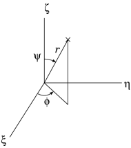
Figure 4. Spherical coordinates.

We next rewrite the Hamiltonian (4.2) in the spherical coordinates. Let

$$x=r\sin\psi\cos\phi,\quad y=r\sin\psi\sin\phi,\quad z=r\cos\psi.$$

See Fig. 4. The momenta $(p_{r},p_{\phi},p_{\psi})$ corresponding to $(r,\phi,\psi)$ satisfy

$$p_{x}=p_{r}\cos\phi\sin\psi-\frac{p_{\phi}\sin\phi}{r\sin\psi}+\frac{p_{\psi}}{r}\cos\phi\cos\psi,$$

$$p_{y}=p_{r}\sin\phi\sin\psi+\frac{p_{\phi}\cos\phi}{r\sin\psi}+\frac{p_{\psi}}{r}\sin\phi\cos\psi,$$

$$p_{z}=p_{r}\cos\psi-\frac{p_{\psi}}{r}\sin\psi$$

(see, e.g., Section 8.7 of [13]). The Hamiltonian becomes

$$H= \tfrac{1}{2}\left(p_{r}^{2}+\frac{p_{\psi}^{2}}{r^{2}}+\frac{p_{\phi}^{2}}{r^{2}\sin^{2}\psi}\right)-\frac{1}{r}-p_{\phi}$$

$$+\mu\biggl{(}\frac{r+\sin\psi\cos\phi}{r^{2}}-\frac{1}{\sqrt{r^{2}+1-2r\sin\psi\cos\phi}}\biggr{)}.$$

When $\mu=0$, the corresponding Hamiltonian system is written as

$$\begin{split}&\dot{r}=p_{r},\quad\dot{p}_{r}=\frac{p_{\psi}^{2}}{r^{3}}+\frac{p_{\phi}^{2}}{r^{3}\sin^{2}\psi}-\frac{1}{r^{2}},\quad\dot{\phi}=\frac{p_{\phi}}{r^{2}\sin^{2}\psi}-1,\\ &\dot{p}_{\phi}=0,\quad\dot{\psi}=\frac{p_{\psi}}{r^{2}},\quad\dot{p}_{\psi}=\frac{p_{\phi}^{2}\cos\psi}{r^{2}\sin^{3}\psi}.\end{split}$$ (4.3)

We also have the relation (3.4) for periodic orbits on the $xy$-plane since Eq. (4.3) reduces to (3.3) there when $\psi=\tfrac{1}{2}\pi$ and $p_{\psi}=0$.

As in the planar case, we introduce the Delaunay elements obtained from the generating function

$$\hat{W}(r,\phi,\psi,I_{1},I_{2}.I_{2})=I_{3}\phi+\chi(r,I_{1},I_{2})+\hat{\chi}(\psi,I_{2},I_{3}),$$ (4.4)

where

$$\hat{\chi}(\psi,I_{2},I_{3})= \int_{\psi_{0}}^{\psi}\left(I_{2}^{2}-\frac{I_{3}^{2}}{\sin^{2}s}\right)^{1/2}\mathrm{d}s$$

$$= I_{2}\arctan\frac{\sqrt{I_{2}^{2}\sin^{2}\psi-I_{3}^{2}}}{I_{2}\cos\psi}-I_{3}\arctan\frac{\sqrt{I_{2}^{2}\sin^{2}\psi-I_{3}^{2}}}{I_{3}\cos\psi}$$ (4.5)

with $\psi_{0}=\arcsin(I_{3}/I_{2})$. See, e.g., Section 8.9.3 of [13], although a slightly modified generating function is used here. We have

$$\begin{split}&p_{r}=\frac{\partial\hat{W}}{\partial r}=\frac{\partial\chi}{\partial r}(r,I_{1},I_{2}),\quad p_{\phi}=\frac{\partial\hat{W}}{\partial\phi}=I_{3},\\ &p_{\psi}=\frac{\partial\hat{W}}{\partial\psi}=\frac{\partial\hat{\chi}}{\partial\psi}(\psi,I_{2},I_{3}),\quad\theta_{1}=\frac{\partial\hat{W}}{\partial I_{1}}=\chi_{1}(r,I_{1},I_{2}),\\ &\theta_{2}=\frac{\partial\hat{W}}{\partial I_{2}}=\chi_{2}(r,I_{1},I_{2})+\hat{\chi}_{2}(\psi,I_{2},I_{3}),\quad\theta_{3}=\frac{\partial\hat{W}}{\partial I_{3}}=\phi+\hat{\chi}_{3}(\psi,I_{2},I_{3}),\end{split}$$ (4.6)

where

$$\hat{\chi}_{2}(\psi,I_{2},I_{3})=\frac{\partial\hat{\chi}}{\partial I_{2}}(\psi,I_{2},I_{3}),\quad\hat{\chi}_{3}(\psi,I_{2},I_{3})=\frac{\partial\hat{\chi}}{\partial I_{3}}(\psi,I_{2},I_{3}).$$

Since the transformation from $(r,\phi,\psi,p_{r},p_{\phi},p_{\psi})$ to $(\theta_{1},\theta_{2},\theta_{3},I_{1},I_{2},I_{3})$ is symplectic, the transformed system is also Hamiltonian and its Hamiltonian is given by

$$H= -\frac{1}{2I_{1}^{2}}-I_{3}+\mu\biggl{(}\frac{1}{R(\theta_{1},I_{1},I_{2})}+\frac{\sin\Psi(\theta_{1},\theta_{2},I_{1},I_{2},I_{3})}{R(\theta_{1},I_{1},I_{2})^{2}}$$

$$\times\cos(\theta_{3}-\hat{\chi}_{3}(\Psi(\theta_{1},\theta_{2},I_{1},I_{2},I_{3}),I_{2},I_{3}))$$

$$-\bigl{(}R(\theta_{1},I_{1},I_{2})^{2}+1-2R(\theta_{1},I_{1},I_{2})\sin\Psi(\theta_{1},\theta_{2},I_{1},I_{2},I_{3})$$

$$\times\cos(\theta_{3}-\hat{\chi}_{3}(\Psi(\theta_{1},\theta_{2},I_{1},I_{2},I_{3}),I_{2},I_{3}))\bigr{)}^{-1/2}\biggr{)},$$ (4.7)

where $r=R(\theta_{1},I_{1},I_{2})$ and $\psi=\Psi(\theta_{1},\theta_{2},I_{1},I_{2},I_{3})$ are the $r$- and $\psi$-components of the symplectic transformation satisfying (3.10) and

$$\hat{\chi}_{2}(\Psi(\theta_{1},\theta_{2},I_{1},I_{2},I_{3}),I_{2},I_{3})+\chi_{2}(R(\theta_{1},I_{1},I_{2}),I_{1},I_{2}))=\theta_{2},$$

respectively. The associated Hamiltonian system is written as

$$\begin{split}&\dot{I}_{1}=\mu h_{1}(I_{1},I_{2},I_{3},\theta_{1},\theta_{2},\theta_{3}),\quad\dot{I}_{2}=O(\mu),\quad\dot{I}_{3}=O(\mu),\\ &\dot{\theta}_{1}=\frac{1}{I_{1}^{3}}+O(\mu),\quad\dot{\theta}_{2}=O(\mu),\quad\dot{\theta}_{3}=-1+O(\mu),\end{split}$$ (4.8)

where

$$h_{1}(I_{1},I_{2},I_{3},\theta_{1},\theta_{2},\theta_{3})$$

$$=\frac{\partial R}{\partial\theta_{1}}(\theta_{1},I_{1},I_{2})\biggl{(}\frac{1}{R(\theta_{1},I_{1},I_{2})^{2}}$$

$$\quad+\frac{2\sin\Psi(\theta_{1},\theta_{2},I_{1},I_{2},I_{3})}{R(\theta_{1},I_{1},I_{2})^{3}}\cos(\theta_{3}-\hat{\chi}_{3}(\Psi(\theta_{1},\theta_{2},I_{1},I_{2},I_{3}),I_{2},I_{3}))$$

$$\quad-\bigl{(}R(\theta_{1},I_{1},I_{2})^{2}+1-2R(\theta_{1},I_{1},I_{2})\sin\Psi(\theta_{1},\theta_{2},I_{1},I_{2},I_{3})$$

$$\quad\times\cos(\theta_{3}-\hat{\chi}_{3}(\Psi(\theta_{1},\theta_{2},I_{1},I_{2},I_{3}),I_{2},I_{3}))\bigr{)}^{-3/2}\biggl{(}R(\theta_{1},I_{1},I_{2})$$

$$\quad-\sin\Psi(\theta_{1},\theta_{2},I_{1},I_{2},I_{3})\cos(\theta_{3}-\hat{\chi}_{3}(\Psi(\theta_{1},\theta_{2},I_{1},I_{2},I_{3}),I_{2},I_{3}))\biggr{)}\biggr{)}$$

$$\quad+\frac{\partial\Psi}{\partial\theta_{1}}(\theta_{1},\theta_{2},I_{1},I_{2},I_{3})\biggl{(}\frac{\sin\Psi(\theta_{1},\theta_{2},I_{1},I_{2},I_{3})}{R(\theta_{1},I_{1},I_{2})^{2}}$$

$$\quad\times\sin(\theta_{3}-\hat{\chi}_{3}(\Psi(\theta_{1},\theta_{2},I_{1},I_{2},I_{3}),I_{2},I_{3}))\frac{\partial\hat{\chi}_{3}}{\partial\psi}(\Psi(\theta_{1},\theta_{2},I_{1},I_{2},I_{3}),I_{2},I_{3}))$$

$$\quad-\frac{\cos\Psi(\theta_{1},\theta_{2},I_{1},I_{2},I_{3})}{R(\theta_{1},I_{1},I_{2})^{2}}\cos(\theta_{3}-\hat{\chi}_{3}(\Psi(\theta_{1},\theta_{2},I_{1},I_{2},I_{3}),I_{2},I_{3}))$$

$$\quad+R(\theta_{1},I_{1},I_{2})\bigl{(}R(\theta_{1},I_{1},I_{2})^{2}+1-2R(\theta_{1},I_{1},I_{2})\sin\Psi(\theta_{1},\theta_{2},I_{1},I_{2},I_{3})$$

$$\quad\times\cos(\theta_{3}-\hat{\chi}_{3}(\Psi(\theta_{1},\theta_{2},I_{1},I_{2},I_{3}),I_{2},I_{3}))\bigr{)}^{-3/2}\biggl{(}\cos\Psi(\theta_{1},\theta_{2},I_{1},I_{2},I_{3})$$

$$\quad\times\cos(\theta_{3}-\hat{\chi}_{3}(\Psi(\theta_{1},\theta_{2},I_{1},I_{2},I_{3}),I_{2},I_{3}))-\sin\Psi(\theta_{1},\theta_{2},I_{1},I_{2},I_{3})$$

$$\quad\times\sin(\theta_{3}-\hat{\chi}_{3}(\Psi(\theta_{1},\theta_{2},I_{1},I_{2},I_{3}),I_{2},I_{3}))\frac{\partial\hat{\chi}_{3}}{\partial\psi}(\Psi(\theta_{1},\theta_{2},I_{1},I_{2},I_{3}),I_{2},I_{3}))\biggr{)}.$$

As in the planar case, we introduce the new variables $w_{1},w_{2}\in(\mathbb{C}/2\pi)$ given by

$$W_{1}(w_{1},\psi,I_{2},I_{3}):=I_{2}^{2}\cos^{2}\psi\tan^{2}w_{1}-I_{2}^{2}\sin^{2}\psi+I_{3}^{2}=0,$$

$$W_{2}(w_{2},\psi,I_{2},I_{3}):=I_{3}^{2}\cos^{2}\psi\tan^{2}w_{2}-I_{2}^{2}\sin^{2}\psi+I_{3}^{2}=0$$

are introduced, so that the generating function (4.4) is regarded as an analytic one on the six–dimensional complex manifold

$$\bar{\mathscr{S}}_{3}= \{(r,\phi,\psi,I_{1},I_{2},I_{3},v_{1},v_{2},v_{3},w_{1},w_{2})\in\mathbb{C}\times(\mathbb{C}/2\pi\mathbb{Z})^{2}\times\mathbb{C}^{4}\times(\mathbb{C}/2\pi\mathbb{Z})^{4}$$

$$\quad\mid V_{j}(v_{j},r,I_{1},I_{2})=W_{l}(w_{l},\psi,I_{2},I_{3})=0,\ j=1,2,3,\ l=1,2\}$$

since Eq. (4.5) is represented by

$$\hat{\chi}(I_{2},I_{3};v_{1},v_{2})=I_{2}w_{1}-I_{3}w_{2}.$$

Moreover, we can regard (4.8) as a meromorphic three-degree-of-freedom Hamiltonian systems on the six-dimensional complex manifold

$$\mathscr{S}_{3}= \{(I_{1},I_{2},I_{3},\theta_{1},\theta_{2},\theta_{3},r,v_{1},v_{2},v_{3},w_{1},w_{2})\in\mathbb{C}^{3}\times(\mathbb{C}/2\pi\mathbb{Z})^{3}\times\mathbb{C}^{2}\times(\mathbb{C}/2\pi\mathbb{Z})^{4}$$

$$\quad\mid\theta_{1}-\chi_{1}(r,I_{1},I_{2})=V_{j}(v_{j},r,I_{1},I_{2})=W_{l}(w_{l},\psi,I_{2},I_{3})=0,$$

$$\qquad j=1,2,3,\ l=1,2\}.$$

Actually, we have

$$\frac{\partial W_{j}}{\partial w_{j}}\frac{\partial w_{j}}{\partial\psi}+\frac{\partial W_{j}}{\partial\psi}=0,\quad\frac{\partial W_{j}}{\partial w_{j}}\frac{\partial w_{j}}{\partial I_{l}}+\frac{\partial W_{j}}{\partial I_{l}}=0,\quad j=1,2,\ l=2,3$$

to express

$$\frac{\partial\hat{\chi}}{\partial\psi}=\sum_{j=1}^{2}\frac{\partial\hat{\chi}}{\partial w_{j}}\frac{\partial W_{j}}{\partial\psi},\quad\hat{\chi}_{l}=\frac{\partial\hat{\chi}}{\partial I_{l}}+\sum_{j=1}^{2}\frac{\partial\hat{\chi}}{\partial w_{j}}\frac{\partial W_{j}}{\partial I_{l}},\quad l=2,3$$

as meromorophic functions of $(\psi,I_{2},I_{3},w_{1},w_{2})$ on $\bar{\mathscr{S}}_{3}$. Let $\Sigma(\mathscr{S}_{3})$ is the critical set of $\mathscr{S}_{3}$ on which the projection $\pi_{3}:\hat{\mathscr{S}}_{3}\to\mathbb{C}^{3}\times(\mathbb{C}/2\pi\mathbb{Z})^{3}$ given by

$$\pi_{3}(I_{1},I_{2},I_{3},\theta_{1},\theta_{2},\theta_{3},r,v_{1},v_{2},v_{3},w_{1},w_{2})=(I_{1},I_{2},I_{3},\theta_{1},\theta_{2},\theta_{3})$$

is singular.

Theorem 4.1.

The Hamiltonian system (3.11) with the Hamiltonian (3.9) does not have a complete set of first integrals in involution that are functionally independent almost everywhere and meromorphic in $(I_{1},I_{2},I_{3},\theta_{1},\theta_{2},\theta_{3},v_{1},v_{2},v_{3},w_{1},w_{2},\mu)$ in a neighborhood of the unperturbed orbit $\{I_{1},I_{2},I_{3}=\text{const.}\}$ with $I_{2}=I_{3}\in(0,I_{1})$ or $(I_{1},0)$ and $I_{1}^{3}\in\mathbb{Q}\setminus\{0\}$ on $\mathscr{S}_{3}\setminus\Sigma(\mathscr{S}_{3})$ near $\mu=0$.

Proof.

We only have to show that the hypotheses of Theorem 2.1 hold for (4.8) as in the proof of Theorem 3.1.

We first estimate $h_{1}(I,\theta)$ for the unperturbed solutions to (4.8). When $\mu=0$, we see that $I_{1},I_{2},I_{3},\theta_{2}$ are constants and can write $\theta_{1}=\omega_{1}t+\theta_{10}$ and $\theta_{3}=-t+\theta_{30}$ for any solution to (4.8) with (3.12), where $\theta_{10},\theta_{30}\in\mathbb{S}^{1}$ are constants. Note that if $\psi=\tfrac{1}{2}\pi$ and $p_{\psi}=0$, then $I_{2}=I_{3}$ by (4.6). Since $r=R(\omega_{1}t+\theta_{10},I_{1},I_{2})$ and

$$\phi=-t-\hat{\chi}_{3}(\Psi(\omega_{1}t+\theta_{10},\theta_{2},I_{1},I_{2}),I_{2},I_{2}),\quad\Psi(\omega_{1}t+\theta_{10},\theta_{2},I_{1},I_{2})=\tfrac{1}{2}\pi,$$

respectively, become the $r$- and $\phi$-components of a solution to (4.3) with $\psi=\tfrac{1}{2}\pi$ and $p_{\psi}=0$, we have the first equation of (3.13) with

$$-\hat{\chi}_{3}(\Psi(\omega_{1}t+\theta_{10},\theta_{2},I_{1},I_{2},I_{2}),I_{2},I_{2})=\phi(t)+t+\bar{\phi}(\theta_{10}),$$ (4.9)

where $\phi(t)$ is the $\phi$-component of a solution to (3.3) and $\bar{\phi}(\theta_{1})$ is a constant depending only on $\theta_{1}$ as in the planar case. Differentiating (4.9) with respect to $t$ yields

$$-\omega_{1}\frac{\partial\hat{\chi}_{3}}{\partial\psi}(\Psi(\omega_{1}t+\theta_{10},\theta_{2},I_{1},I_{2},I_{2}),I_{2},I_{2})$$

$$\qquad\times\frac{\partial\Psi}{\partial\theta_{1}}(\omega_{1}t+\theta_{10},\theta_{2},I_{1},I_{2},I_{2})=\dot{\phi}(t)+1.$$ (4.10)

Fix $I_{1}=I_{1}^{\ast}$ such that $\omega_{1}=k_{1}/k_{2}$ for $k_{1},k_{2}>0$ relatively prime integers, i.e., $I_{1}^{\ast 3}=k_{2}/k_{1}\in\mathbb{Q}$. The following arguments can be modified to apply when $\omega_{1}<0$, as in Section 3. Assumption (A1) holds with $\omega^{\ast}=1/k_{2}$ as in Section 3. By (4.9) $\phi(t)$ is $2\pi k_{2}/k_{1}$-periodic, so that by (3.5)

$$I_{2}=I_{3}=I_{1}^{\ast}\sqrt{1-\varepsilon^{2}}\ (=:I_{2}^{\ast}).$$

From (3.12) we have

$$\mathrm{D}\omega(I^{\ast})=\begin{pmatrix}-3/I_{1}^{\ast 4}&0&0\\ 0&0&0\\ 0&0&0\end{pmatrix},$$

where $I=I^{\ast}:=(I_{1}^{\ast},I_{2}^{\ast},I_{2}^{\ast})$. Using the first equations of (3.13) and (3.14), (4.9) and (4.10), we obtain

$$h_{1}(I^{\ast},\tau+\theta_{1},\theta_{2},-\tau+\theta_{3})\mathrm{d}\tau$$

$$=\frac{k_{2}\dot{\varphi}(t)}{k_{1}}\biggl{(}\frac{e}{I_{2}^{\ast 2}}\sin\varphi(t)+\frac{2e}{I_{2}^{\ast 4}}(1+e\cos\varphi(t))\sin\varphi(t)\cos(\phi(t)+\theta_{3})$$

$$\quad+\frac{1}{I_{2}^{\ast 4}}(1+e\cos\varphi(t))^{2}\sin(\phi(t)+\theta_{3})$$

$$\quad-\frac{1}{\hat{r}(t;\theta_{3})^{3}}\biggl{(}eI_{2}^{\ast 4}\sin\varphi(t)+I_{2}^{\ast 2}(1+e\cos\varphi(t))^{2}\sin(\phi(t)+\theta_{3}$$

$$\quad-eI_{2}^{\ast 2}(1+e\cos\varphi(t))\sin\varphi(t)\cos(\phi(t)+\theta_{3})\biggr{)}$$ (4.11)

after an appropriate shift of the time variable $t$, where $\hat{r}(t;\theta_{3})$ is given by (3.17) with $\theta_{2}=\theta_{3}$. Equation (4.11) has the same expression as (3.16) with $\theta_{2}=\theta_{3}$. Repeating the arguments in the proof of Theorem 3.1, we can show that assumption (A2) holds as in the planar case. Thus, we use Theorem 2.1 to complete the proof. ∎

Remark 4.2.

From the above proof we see that the planar problem (1.2) is nonintegrable near the periodic orbits

$$r=\frac{(k_{2}/k_{1})^{2/3}(1-e^{2})}{1+e\cos(\varphi(t)+\bar{\phi})},\quad t\in\mathbb{C},$$

on the $xy$-plane, for any $e\in(0,1)$, $\bar{\phi}\in\mathbb{S}^{1}$ and $(k_{1},k_{2})$ of relatively prime positive integers, where $\varphi(t)$ is implicitly given by (3.19), as in Remark 3.2.

Data Availability

Data sharing not applicable to this article as no dataset was generated or analyzed during the current study.

References

• [1] V.I. Arnold, Mathematical Methods of Classical Mechanics, 2nd ed., Springer, New York, 1989.
• [2] V. I. Arnold, V.V. Kozlov and A.I. Neishtadt, Dynamical Systems III: Mathematical Aspects of Classical and Celestial Mechanics, 3rd ed., Springer, Berlin, 2006.
• [3] M. Ayoul and N.T. Zung, Galoisian obstructions to non-Hamiltonian integrability, C. R. Math. Acad. Sci. Paris, 348 (2010), 1323–1326.
• [4] J. Barrow-Green, Poincaré and the Three-Body Problem, American Mathematical Society, Providence, RI, 1996.
• [5] O.I. Bogoyavlenskij, Extended integrability and bi-hamiltonian systems, Comm. Math. Phys., 196 (1998), 19–51.
• [6] D. Boucher, Sur la non-intégrabilité du problème plan des trois corps de masses égales, C. R. Acad. Sci. Paris Sér. I Math.,331 (2000), 391–394.
• [7] D. Boucher and J.-A. Weil, Application of J.-J. Morales and J.-P. Ramis’ theorem to test the non-complete integrability of the planar three-body problem, in F. Fauvet and C. Mitschi (eds.), From Combinatorics to Dynamical Systems, de Gruyter, Berlin, 2003, pp.163–177.
• [8] T. Combot, A note on algebraic potentials and Morales-Ramis theory, Celestial Mech. Dynam. Astronom., 115 (2013), 397–404.
• [9] M. Guardia, P. Martín and T.M. Seara, Oscillatory motions for the restricted planar circular three body problem, Invent. Math., 203 (2016), 417–492.
• [10] V.V. Kozlov, Integrability and non-integarbility in Hamiltonian mechanics, Russian Math. Surveys, 38 (1983), 1–76.
• [11] V.V. Kozlov, Symmetries, Topology and Resonances in Hamiltonian Mechanics, Springer, Berlin, 1996.
• [12] J. Llibre and C. Simó, Oscillatory solutions in the planar restricted three-body problem, Math. Ann., 248 (1980), 153–184.
• [13] K.R. Meyer and D.C. Offin, Introduction to Hamiltonian Dynamical Systems and the N-Body Problem, 3rd ed., Springer, 2017.
• [14] J.J. Morales-Ruiz, Differential Galois Theory and Non-Integrability of Hamiltonian Systems, Birkhäuser, Basel, 1999.
• [15] J.J. Morales-Ruiz and J.-P. Ramis, Galoisian obstructions to integrability of Hamiltonian systems, Methods, Appl. Anal., 8 (2001), 33–96.
• [16] J.J. Morales-Ruiz, J.-P. Ramis and C. Simo, Integrability of Hamiltonian systems and differential Galois groups of higher variational equations, Ann. Sci. École Norm. Suppl., 40 (2007), 845–884.
• [17] J.J. Morales-Ruiz and S. Simon, On the meromorphic non-integrability of some $N$-body problems, Discret.Contin. Dyn. Syst., 24 (2009), 1225–1273.
• [18] J. Moser, Stable and Random Motions in Dynamical Systems, Princeton University Press, Princeton, 1973.
• [19] H. Poincaré, Sur le probléme des trois corps et les équations de la dynamique, Acta Math., 13 (1890), 1–270; English translation: The Three-Body Problem and the Equations of Dynamics, Translated by D. Popp, Springer, Cham, Switzerland, 2017.
• [20] H. Poincaré, New Methods of Celestial Mechanics, Vol. 1, AIP Press, New York, 1992 (original 1892).
• [21] A. Tsygvintsev, La non-intégrabilité méromorphe du problème plan des trois corps, C. R. Acad. Sci. Paris Sér. I Math.,331 (2000), 241–244.
• [22] A. Tsygvintsev, The meromorphic non-integrability of the three-body problem, J. Reine Angew. Math., 537 (2001), 127–149.
• [23] A. Tsygvintsev, Sur l’absence d’une intégrale premir̀e mŕomorphe supplémentaire dans le probléme plan des trois corps, C. R. Acad. Sci. Paris Sér. I Math.,333 (2001), 125–128.
• [24] A. Tsygvintsev, Non-existence of new meromorphic first integrals in the planar three-body problem, Celestial Mech. Dynam. Astronom., 86 (2003), 237–247.
• [25] A. Tsygvintsev, On some exceptional cases in the integrability of the three-body problem, Celestial Mech. Dynam. Astronom., 99 (2007), 23–29.
• [26] E.T. Whittaker, A Treatise on the Analytical Dynamics of Particles and Rigid Bodies, 3rd ed., Cambridge University Press, Cambridge, 1937.
• [27] Z. Xia, Mel’nikov method and transversal homoclinic points in the restricted three-body problem, J. Differential Equations, 96 (1992), 170–184.
• [28] K. Yagasaki, Nonintegrability of the restricted three-body problem, submitted for publication. arXiv:2106.04925 [math.DS]
• [29] K. Yagasaki, Nonintegrability of nearly integrable dynamical systems near resonant periodic orbits, submitted for publication. arXiv:2106.04930 [math.DS]
• [30] S.L. Ziglin, Bifurcation of solutions and the nonexistence of first integrals in Hamiltonian mechanics. I. Funct. Anal. Appl., 16 (1982), 181–189.
• [31] S.L. Ziglin, On involutive integrals of groups of linear symplectic transformations and natural mechanical systems with homogeneous potential, Funct. Anal. Appl., 34 (2000), 179–187.
• [32] N.T. Zung, A conceptual approach to the problem of action-angle variables, Arch. Ration. Mech. Anal., 229 (2018), 789–833.