The roughness exponent and its model-free estimation

Abstract

Motivated by pathwise stochastic calculus, we say that a continuous real-valued function $x$ admits the roughness exponent $R$ if the $p^{\text{th}}$ variation of $x$ converges to zero for $p>1/R$ and to infinity for $p<1/R$. In our main result, we provide a mild condition on the Faber–Schauder coefficients of $x$ under which the roughness exponent exists and is given as the limit of the classical Gladyshev estimates $\widehat{R}_{n}(x)$. This result can be viewed as a strong consistency result for the Gladyshev estimators in an entirely model-free setting, because no assumption whatsoever is made on the possible dynamics of the function $x$. Nonetheless, our proof is probabilistic and relies on a martingale hidden in the Faber–Schauder expansion of $x$. We show that the condition of our main result is satisfied for the typical sample paths of fractional Brownian motion with drift, and we provide almost-sure convergence rates for the corresponding Gladyshev estimates. We also discuss the connections between the roughness exponent and the related concepts of Besov regularity and weighted quadratic variation. Since the Gladyshev estimators are not scale-invariant, we construct several scale-invariant estimators. Finally, we extend our results to the case in which the $p^{\text{th}}$ variation of $x$ is defined over a sequence of unequally spaced partitions.

MSC2020 subject classifications: 60F15, 60G22, 60G46, 62G05, 26A30

Keywords. Roughness exponent, power variation, Gladyshev estimator, Faber–Schauder system, fractional Brownian motion with drift, Besov regularity, weighted quadratic variation

1 Introduction

The Hurst parameter was originally defined by Hurst [20] as a measure of the autocorrelation of a time series. But it is well known that it can also determine the degree of ‘roughness’ of a trajectory, e.g., in terms of the fractal dimension of its graph. Both notions are often used interchangeably in the literature. While the link between autocorrelation and roughness is well-established for stochastic processes such as fractional Brownian motion, it is by no means a universal truth. Indeed, Gneiting and Schlather [15] constructed a class of stationary Gaussian processes for which the Hurst parameter and fractal dimension decouple completely; see also Cheridito [3] and Bennedsen et al. [2]. It is therefore necessary to distinguish between the classical, autocorrelation-based Hurst parameter and a suitable index for the roughness of a trajectory. In this paper, we study such a roughness index, which is based on the $p^{\text{th}}$ variation of a continuous real-valued function.

Recall that, if $x:[0,1]\to{\mathbb{R}}$ is a continuous function and $p>0$, the $p^{\text{th}}$ variation of $x$ along the sequence of dyadic partitions is defined as the limit of

$$\langle x\rangle_{n}^{(p)}:=\sum_{k=0}^{2^{n}-1}\big{|}x((k+1)2^{-n})-x(k2^{-n})\big{|}^{p},$$

provided that this limit exists. We will say that $x$ admits the roughness exponent $R\in[0,1]$ if

$$\lim_{n\uparrow\infty}\langle x\rangle_{n}^{(p)}=\begin{cases}0&\quad\text{for $p>1/R$},\\ \infty&\quad\text{for $p<1/R$}.\end{cases}$$ (1.1)

Intuitively, the smaller $R$, the rougher the trajectory $x$ will look. For instance, if $x$ is continuously differentiable, then (1.1) holds with $R=1$, and this is also the largest possible value for $R$ unless $x$ is constant. If $x$ is a typical sample path of a continuous semimartingale such as Brownian motion, then (2.2) holds with $R=1/2$. If $x$ is a typical sample path of fractional Brownian motion, then $R$ is equal to its classical Hurst parameter.

When measuring the roughness of a trajectory, there are strong reasons for favouring $p^{\text{th}}$ variation over other measures such as fractal dimension. First, the $p^{\text{th}}$ variation can be measured in a straightforward manner. Second, other measures may lead to diverging results, and there is no canonical choice. For instance, the graph of a trajectory may have different Hausdorff and box dimensions. Third, and probably most importantly, the $p^{\text{th}}$ variation plays a crucial role in the extension of Itô calculus to rough trajectories. A pathwise and strictly model-free version of such an extension for integrators with arbitrary $p^{\text{th}}$ variation was recently established by Cont and Perkowski [7]. Itô calculus for rough trajectories also plays an important role in applications, for instance to rough volatility models. These models are based on the observation by Gatheral et al. [13] that the Hurst parameter of the realized volatility of many financial time series is rather small, which makes realized volatility much rougher than the sample paths of a continuous semimartingale.

In Theorem 2.4, our main result, we establish the existence of the roughness exponent under a mild condition on the Faber–Schauder coefficients of $x$. We call this condition the reverse Jensen condition. Even more important than the existence of the roughness exponent is the fact that the reverse Jensen condition guarantees that the roughness exponent of $x$ can be obtained as the limit of the classical Gladyshev estimates $\widehat{R}_{n}(x)$. This part of Theorem 2.4 can be viewed as a strong consistency result for the Gladyshev estimators in an entirely model-free setting, because no assumption whatsoever is made on the possible dynamics of the function $x$. In particular, we do not assume that $x$ can be obtained as a sample path of some stochastic process, even though this is clearly the typical application we have in mind. While the statement of Theorem 2.4 appears to be deterministic, its proof is probabilistic. It relies on martingale techniques that are applied to a martingale that is hidden in the Faber–Schauder expansion of $x$. The corresponding theory is developed in Section 3, where also the proof of Theorem 2.4 is given.

The Gladyshev estimator has traditionally been used to estimate the Hurst parameter of stochastic processes such as fractional Brownian motion. So one conceptual contribution of Theorem 2.4 is the observation that the Gladyshev estimator actually estimates the roughness exponent and that its limit only delivers the classical Hurst parameter if and only if the latter coincides with the former. This is the case for fractional Brownian motion, which is the subject of Section 5. Our main result in this section, Theorem 5.1, shows in particular that the typical sample paths of fractional Brownian motion with drift satisfy the reverse Jensen condition. Additionally, it provides almost-sure convergence rates for the corresponding Gladyshev estimates.

The Gladyshev estimator was originally derived from Gladyshev’s theorem [14], which is an almost-sure limit theorem for the weighted quadratic variation of certain Gaussian processes. In Section 4 we systematically investigate the relations between weighted quadratic variation and the roughness exponent. In particular, we show that for any continuous function the existence of the weighted quadratic variation is strictly stronger than the convergence of the Gladyshev estimates. However, we also provide an example of a function for which the parameter derived from the weighted quadratic variation is different from the roughness exponent.

Due to a result by Rosenbaum [32], the existence of the weighted quadratic variation is in turn closely related to the concept of Besov regularity. In Section 6, we systematically analyze relations between variants of this concept and the existence of a roughness parameter. First, we observe that Eyink’s formulation of Besov regularity [9] leads to a roughness concept that is generally different from ours. Then we examine somewhat more restrictive requirement, which is sometimes proposed in the rough volatility context. Our main result in this section, Theorem 6.2, links the corresponding roughness measure to $p^{\text{th}}$ variations. However, Example 6.3 shows that even this concept of Besov regularity does not imply the existence of a roughness exponent.

The results in Sections 4 and 6 hold also if the reverse Jensen condition is not assumed. In Section 7 we collect several additional results that are also valid in this more general context.

In Section 8, we discuss the problem of estimating the roughness exponent from discrete observations of a given function $x$. Here, the fact that the Gladyshev estimator is not scale-invariant can become an issue. We therefore provide several families of scale-invariant estimators that are derived from the sequence $(\widehat{R}_{n})_{n\in\mathbb{N}}$ without deteriorating the corresponding rate of convergence. We also relate the estimator used in [13] to those families.

In LABEL:irregularsection, we provide an extension of our main results to the case in which the $p^{\text{th}}$ variation is defined over a sequence of unequally spaced partitions.

2 The roughness exponent: definition and existence

Let $x:[0,1]\to{\mathbb{R}}$ be any fixed continuous function. This function can be a natural or economic time series, a typical sample path of a stochastic process, or a fractal function. What these phenomena have in common is that the corresponding trajectories are not smooth but exhibit a certain degree of ‘roughness’. In the sequel, our goal is to quantify and measure the degree of that roughness. To this end, we will henceforth exclude the trivial case of a constant function $x$.

For $p>0$ and $n\in\mathbb{N}$, we define

$$\langle x\rangle_{n}^{(p)}:=\sum_{k=0}^{2^{n}-1}\big{|}x((k+1)2^{-n})-x(k2^{-n})\big{|}^{p},$$ (2.1)

which can be regarded as the $p^{\text{\rm th}}$ variation of the function $x$ sampled along the dyadic partition $\{k2^{-n}:k=0,\dots,2^{n}\}$. Suppose that there exists $q$ such that

$$\lim_{n\uparrow\infty}\langle x\rangle_{n}^{(p)}=\begin{cases}0&\quad\text{for $p>q$},\\ \infty&\quad\text{for $p<q$}.\end{cases}$$ (2.2)

Intuitively, the larger $q$, the rougher the trajectory $x$ will look. For instance, if $x$ is continuously differentiable, then (2.2) holds with $q=1$, and this is also the smallest possible value for $q$, because $x$ is nonconstant by assumption. Moreover, it is easy to see that (1.1) holds if $\lim_{n}\langle x\rangle^{(p)}_{n}$ exists in $(0,\infty)$ (see, e.g., the final step in the proof of Theorem 2.1 in [29]). In particular, if $x$ is a typical sample path of a continuous semimartingale such as Brownian motion, then (2.2) holds with $q=2$. More generally, if $x$ is a typical sample path of a fractional Brownian motion with Hurst parameter $H\in(0,1)$, then $q$ is equal to $1/H$; see Theorem 5.1 and the subsequent paragraph. The extreme case $q=\infty$ implies that $\langle x\rangle^{(p)}_{n}$ diverges to infinity for any $p\geq 1$; an example is provided in Example 2.9.

Definition 2.1.

Suppose that there exists $q\in[1,\infty]$ such that (2.2) holds. Then $R:=1/q$ is called the roughness exponent of $x\in C[0,1]$.

A concept closely related to the roughness exponent was used by Gatheral et al. [13] to quantify the roughness of empirical volatility time series. In [29], [17] and [18], the roughness exponent was computed for certain families of fractal functions. The standard Hurst parameter, on the other hand, is defined via the autocorrelation of the time series and measures the amount of long-range dependence in the data. For many stochastic processes, including fractional Brownian motion, the standard Hurst parameter coincides with the roughness exponent of the sample paths. In general, however, these two parameters may be different; for a discussion, see Gneiting and Schlather [15], where roughness is measured in terms of fractal dimension. Later, Bennedsen et al. [2] adopted this idea to study the bifurcation of the short- and long-term behaviour of stochastic volatility with the goal of proposing a new class of stochastic volatility models that can simultaneously incorporate roughness and slowly decaying autocorrelation. Finally, the concept of Besov regularity, introduced by Eyink [9] within the framework of Besov spaces, is somewhat related to our roughness exponent. The corresponding connections are explored in Section 6.

Note that if $x$ admits the roughness exponent $R$, then (2.2) does not make any assertion on the existence of $\lim_{n}\langle x\rangle_{n}^{(p)}$ for $p:=1/R$. This limit always exists for $p=1$ and is equal to the total variation of $x$. For $p>1$, however, the limit may or may not exist (see Example 4.3). If it does exist, it can be interpreted as the $p^{\text{th}}$ variation of the continuous function $x$ along the sequence of dyadic partitions of $[0,1]$. This $p^{\text{th}}$ variation can be used so as to prove a strictly pathwise version of Itô calculus, an approach that was pioneered by Föllmer [11] for $p\leq 2$ and recently extended to $p>2$ by Cont and Perkowski [7]. Just as this notion of $p^{\text{th}}$ variation, the roughness exponent of a trajectory will typically depend on the underlying partition sequence. As noted above, we have chosen here the dyadic partitions, because equally-spaced partitions are natural for many data sources and also lead to the simplest and most elegant mathematical statements. An extension to unequally spaced partitions is provided in Section 9.

There exist continuous functions that do not admit a roughness exponent; see Example 6.3. For this reason, we will first establish criteria for the existence of $R$. Let us start by defining

$$q_{*}:=\sup\Big{\{}p>0:\liminf_{n\uparrow\infty}\langle x\rangle_{n}^{(p)}=\infty\Big{\}}\quad\text{and}\quad q^{*}:=\sup\Big{\{}p>0:\limsup_{n\uparrow\infty}\langle x\rangle_{n}^{(p)}=\infty\Big{\}}.$$ (2.3)

The proof of Proposition 2.2 will show that the following alternative formulas hold for $q_{*}$ and $q^{*}$,

$$q_{*}=\inf\Big{\{}p\geq 1:\liminf_{n\uparrow\infty}\langle x\rangle_{n}^{(p)}=0\Big{\}}\quad\text{and}\quad q^{*}=\inf\Big{\{}p\geq 1:\limsup_{n\uparrow\infty}\langle x\rangle_{n}^{(p)}=0\Big{\}}.$$ (2.4)

Proposition 2.2.

The roughness exponent of $x\in C[0,1]$ exists if and only if $q^{*}=q_{*}$. In this case, $R$ is given by $R=1/q^{*}=1/q_{*}$.

Proof.

Clearly, $R$ is nonnegative by definition. Moreover, since the function $x$ is non-constant by assumption, we have $\langle x\rangle_{n}^{(p)}\to\infty$ for all $p<1$. Hence, we must have $R\leq 1$.

The remaining assertion follows easily from the alternative representation (2.4) of $q_{*}$ and $q^{*}$, so it is sufficient to establish (2.4). To prove this result for the case $q_{*}<\infty$, let $q_{0}:=\inf\{p\geq 1:\liminf_{n\uparrow\infty}\langle x\rangle_{n}^{(p)}=0\}$. Let $n_{0}$ be such that $\max_{k}|x((k+1)2^{-n})-x(k2^{-n})|\leq 1$ for $n\geq n_{0}$. Then $p\mapsto\langle x\rangle_{n}^{(p)}$ is non-increasing for $n\geq n_{0}$, and so we must have $q_{*}\leq q_{0}$. To show the converse inequality, we show that $\liminf_{n}\langle x\rangle_{n}^{(p)}=0$ for every $p>q_{*}$. To this end, we assume by way of contradiction that there exists $p>q_{*}$ such that $v:=\liminf_{n}\langle x\rangle_{n}^{(p)}>0$. The definition of $q_{*}$ implies that we must have $v<\infty$. Next, for any $\varepsilon>0$, there exists $n_{1}\in\mathbb{N}$ such that $\max_{k}|x((k+1)2^{-n})-x(k2^{-n})|\leq\varepsilon$ for $n\geq n_{1}$. Thus, for $q\in(q_{*},p)$ and $n\geq n_{1}$,

$$\langle x\rangle_{n}^{(p)}\leq\max_{k}\big{|}x((k+1)2^{-n})-x(k2^{-n})\big{|}^{p-q}\cdot\langle x\rangle_{n}^{(q)}\leq\varepsilon^{p-q}\langle x\rangle_{n}^{(q)}.$$

When sending $\varepsilon\downarrow 0$, we see that $0<v\leq\varepsilon^{p-q}\liminf_{n}\langle x\rangle_{n}^{(q)}$ for all $\varepsilon>0$. This implies that $\liminf_{n}\langle x\rangle_{n}^{(q)}=\infty$, which, in view of $q>q_{*}$, contradicts the definition of $q_{*}$. This establishes $q_{0}=q_{*}$. If $q_{*}=\infty$, then for each $p>0$, we must have $\liminf_{n\uparrow\infty}\langle x\rangle_{n}^{(p)}=\infty$. Thus, $\{p\geq 1:\liminf_{n\uparrow\infty}\langle x\rangle_{n}^{(p)}=0\}=\emptyset$, which establishes the first identity in (2.4) for the case $q_{*}=\infty$. The second identity in (2.4) is proved in the same manner. ∎

Our analysis of the roughness exponent is based on the Faber–Schauder wavelet expansion of continuous functions. Recall that the Faber–Schauder functions are defined as

$$e_{\emptyset}(t):=t,\quad e_{0,0}(t):=(\min\{t,1-t\})^{+},\quad e_{m,k}(t):=2^{-m/2}e_{0,0}(2^{m}t-k)$$

for $t\in{\mathbb{R}}$, $m\in\mathbb{N}$ and $k\in\mathbb{Z}$. It is well known that the restriction of the Faber–Schauder functions to $[0,1]$ form a Schauder basis for $C[0,1]$. More precisely, every function $x\in C[0,1]$ can be uniquely represented by the following uniformly convergent series,

$$x=x(0)+\left(x(1)-x(0)\right)e_{\emptyset}+\sum_{m=0}^{\infty}\sum_{k=0}^{2^{m}-1}\theta_{m,k}e_{m,k},$$ (2.5)

where the Faber–Schauder coefficients $\theta_{m,k}$ are given by

$$\theta_{m,k}=2^{m/2}\left(2x\Big{(}\frac{2k+1}{2^{m+1}}\Big{)}-x\Big{(}\frac{k}{2^{m}}\Big{)}-x\Big{(}\frac{k+1}{2^{m}}\Big{)}\right).$$

We furthermore denote for $n\in\mathbb{N}$,

$$s_{n}:=\sqrt{\sum_{m=0}^{n-1}\sum_{k=0}^{2^{m}-1}\theta^{2}_{m,k}},\quad\text{and}\quad\widehat{R}_{n}(x):=1-\frac{1}{n}\log_{2}s_{n}.$$ (2.6)

Our main thesis in this paper is that the roughness exponent of $x$ should be equal to the limit of $\widehat{R}_{n}(x)$, provided this limit exists. Theorem 2.4 will rigorously establish this result under the following mild condition on the Faber–Schauder coefficients of $x$. To formulate this and related conditions, we will say that a function $\varrho:{\mathbb{R}}_{+}\to{\mathbb{R}}_{+}$ is subexponential if $\frac{1}{t}\log\varrho(t)\to 0$ as $t\uparrow\infty$.

Definition 2.3.

The Faber–Schauder coefficients of $x$ satisfy the reverse Jensen condition if for each $p\geq 1$ there exist $n_{p}\in\mathbb{N}$ and a non-decreasing subexponential function $\varrho_{p}:\mathbb{N}\rightarrow[1,\infty)$ such that

$$\frac{1}{\varrho_{p}(n)}s_{n}^{p}\leq\frac{1}{2^{n-1}}\sum_{k=0}^{2^{n-1}-1}\Big{(}\sum_{m=0}^{n-1}2^{m}\theta^{2}_{m,\lfloor 2^{m-n+1}k\rfloor}\Big{)}^{p/2}\leq\varrho_{p}(n)s_{n}^{p}\qquad\text{for $n\geq n_{p}$}.$$ (2.7)

If $p\geq 2$, then Jensen’s inequality implies that the left-hand inequality in (2.7) holds with $\varrho_{p}=1$. Likewise, the upper bound holds with $\varrho_{p}=1$ if $p\leq 2$. So only the other cases are nontrivial, which explains our terminology “reverse Jensen condition”. This terminology will become even clearer in Remark 3.3, where an equivalent probabilistic formulation is given. As we are going to see in Theorem 5.1, the reverse Jensen condition is satisfied for the typical sample paths of fractional Brownian motion with arbitrary Hurst parameter. Moreover, two alternative conditions that are easier to verify, but are also stronger, will be provided in Proposition 3.6. Now we can state our first main result, which establishes the existence of the roughness exponent and its relation to the limit of the sequence $\widehat{R}_{n}(x)$ under the assumption that the reverse Jensen condition holds. The second part of Theorem 2.4 states that condition (2.7) at $p=1/R$ is necessary for the convergence of $\widehat{R}_{n}(x)$ to the roughness exponent $R$.

Theorem 2.4.

Suppose that the Faber–Schauder coefficients of $x$ satisfy the reverse Jensen condition. Then the function $x$ admits a roughness exponent $R$ if and only if the finite limit $\lim_{n}\widehat{R}_{n}(x)$ exists, and in this case we have $\widehat{R}_{n}(x)\to R$. Conversely, suppose that $\widehat{R}_{n}(x)$ converges to the roughness exponent $R$ of $x$. Then (2.7) holds at $p=1/R$.

Theorem 2.4 will be proved in the subsequent Section 3. It can be regarded as a model-free consistency result for the estimator $\widehat{R}_{n}$ of the roughness exponent of the continuous function $x$. It has the following two aspects.

First, Theorem 2.4 is model-free in the sense that no assumptions are made on $x$ except the reverse Jensen condition. In particular, we do not assume that $x$ is a realization of a stochastic process with prescribed dynamics, even though this is clearly the typical application we have in mind. This line of thought is similar in spirit to the model-free approach to stochastic analysis, which was pioneered by Föllmer [11] and Lyons [25]. In this approach, one derives results for deterministic trajectories satisfying certain sample path properties, thus avoiding other implicit assumptions (e.g., a Lévy-type modulus of continuity or a law of the iterated logarithm) usually imposed through fixing a probabilistic model. The results can then be applied to all probabilistic models whose trajectories satisfy the assumed sample path properties almost surely. In our analysis of fractional Brownian motion with drift (Section 5) we follow precisely this recipe. We show that almost all of the sample paths satisfy the reverse Jensen condition and we identify the Hurst parameter $H$ as the common roughness exponent of the trajectories. We also provide almost sure convergence rates for the convergence of $\widehat{R}_{n}$ to $H$.

Second, based on the work by Gladyshev [14], it has long been known that $\widehat{R}_{n}$, which is sometimes called the Gladyshev estimator, estimates the Hurst parameter for fractional Brownian motion and other Gaussian processes; see, e.g., [24] for an overview. Theorem 2.4 now clarifies that $\widehat{R}_{n}$ is actually an estimator for the roughness exponent; it estimates the classical Hurst parameter $H$ only if $H$ coincides with the roughness exponent. Our theorem thus demonstrates that the Gladyshev estimator has in fact a much wider scope of possible applications, provided that it is correctly understood as an estimator of the roughness exponent and not of the Hurst parameter. The same is true for certain variants of the Gladyshev estimator such as the scale-invariant modifications discussed in Section 8.

The statement of Theorem 2.4 may become false if the reverse Jensen condition is not satisfied; see Proposition 4.4 for a counterexample. However, as shown by the next result, an exception occurs for functions $x$ that display diffusive behavior in the sense that they admit the roughness exponent $R=1/2$. This includes in particular the typical sample paths of any continuous semimartingale with nontrivial martingale component.

Corollary 2.5.

Let $x\in C[0,1]$ be any function with roughness exponent $1/2$. Then $\lim_{n}\widehat{R}_{n}(x)=1/2$.

The preceding corollary will follow immediately from Proposition 7.1. The following remark outlines what can be shown if the reverse Jensen condition holds but $\widehat{R}_{n}(x)$ does not converge to a limit.

Remark 2.6.

Suppose that the reverse Jensen condition holds and let us denote

$$r^{+}:=\limsup_{n\uparrow\infty}\widehat{R}_{n}(x)\quad\text{and}\quad r^{-}:=\liminf_{n\uparrow\infty}\widehat{R}_{n}(x).$$ (2.8)

One can show as in the proof of Theorem 2.4 that

$$\limsup_{n\uparrow\infty}\langle x\rangle_{n}^{(p)}=\begin{cases}0&\text{if }p>1/r^{-},\\ \infty&\text{if }p<1/r^{-},\\ \end{cases}\qquad\qquad\liminf_{n\uparrow\infty}\langle x\rangle_{n}^{(p)}=\begin{cases}0&\text{if }p>1/r^{+},\\ \infty&\text{if }p<1/r^{+}.\\ \end{cases}$$

To wit, under the reverse Jensen condition, we have $q^{\ast}=1/r^{-}$ and $q_{\ast}=1/r^{+}$. By Proposition 2.2, the roughness exponent is well defined if and only if $r^{+}=r^{-}$, and this special case is discussed in Theorem 2.4; on the other hand, if $r^{+}>r^{-}$, the roughness exponent does not exist, and the sequence $(\langle x\rangle_{n}^{(p)})_{n\in\mathbb{N}_{0}}$ will fluctuate between zero and infinity for any $p\in(1/r^{+},1/r^{-})$.

Remark 2.7.

Suppose $x\in C[0,1]$ is such that its Faber–Schauder coefficients $\theta_{m,k}$ are the same for all $k$. Then the reverse Jensen condition is trivially satisfied. These functions form the so-called Takagi class [19], and, beginning with the subsequent Examples 2.8 and 2.9, several of our examples and counterexamples will belong to this class. The two Examples 2.8 and 2.9 will in particular present for every $R\in[0,1]$ a function $x$ that satisfies the reverse Jensen condition and has roughness exponent $R$.

Example 2.8.

For $\alpha\in(-\sqrt{2},\sqrt{2})$, consider the function with Faber–Schauder coefficients $\theta_{m,k}=\alpha^{m}$. These functions are often called the Takagi–Landsberg functions. For $|\alpha|>1/\sqrt{2}$, it follows from [29, Theorem 2.1] that their roughness exponent is given by $R=\frac{1}{2}-\log_{2}|\alpha|$. Our Theorem 2.4 provides a very short proof of this fact: since

$$s_{n}^{2}=\sum_{m=0}^{n-1}\sum_{k=0}^{2^{m}-1}\alpha^{2m}=\frac{(2\alpha^{2})^{n}-1}{2\alpha^{2}-1},$$

we have $\frac{1}{n}\log_{2}s_{n}\to\frac{1}{2}\log_{2}(2\alpha^{2})=\frac{1}{2}+\log_{2}|\alpha|$, which yields the claim. For $|\alpha|<1/\sqrt{2}$, we get in the same way that $s_{n}^{2}\to(1-2\alpha^{2})^{-1}$. It will be shown in Proposition 7.3 (a) that $x$ must hence be of bounded variation. Finally, in the case $|\alpha|=1/\sqrt{2}$, we have $s_{n}^{2}=n$, which also leads to $R=1$. However, in this case, $x$ is the classical Takagi function, which is nowhere differentiable and hence not of bounded variation; see Remark 2.2 (i) in [33] for details.

On the other extreme end of the spectrum are functions with roughness exponent $R=0$. Such a function is constructed in the following example.

Example 2.9.

Consider the function with Faber–Schauder coefficients $\theta_{m,k}=2^{m/2}(m+1)^{-2}$. One easily checks that this choice gives rise to a well-defined continuous function. As in [18, Proposition 3.1], one can show that $\langle x\rangle_{n}^{(p)}\to\infty$ for all $p\geq 1$. It follows that $q_{*}$ and $q^{*}$, as defined in (2.3), are both infinite, and so Proposition 2.2 yields $R=0$.

In the following Section 3, we present the proof of Theorem 2.4. It is based on a martingale that is hidden in the Faber–Schauder expansion of a continuous function $x$.

3 A martingale hidden in the Faber–Schauder expansion of a continuous function

In this section, we use martingale techniques so as to develop the probabilistic tools for our analysis of the roughness exponent and we will prove Theorem 2.4. The idea of using a probabilistic approach to the $p^{\text{\rm th}}$ variation of functions goes back to [29, 33], where it was used for for certain fractal functions. For a general function $x\in C[0,1]$, however, the tools from [29, 33] are no longer sufficient; see Remark 3.2.

Let $(\Omega,{\mathscr{F}},{\mathbb{P}})$ be a probability space supporting an i.i.d. sequence $(U_{n})_{n\in\mathbb{N}}$ of $\{0,1\}$-valued random variables with symmetric Bernoulli distribution. Furthermore, we define the stochastic processes

$$V_{0}:=0,\quad V_{m}:=\sum_{k=1}^{m}2^{-k}U_{k}\quad\text{and}\quad S_{m}:=2^{m}\theta^{2}_{m,2^{m}V_{m}},\quad m\in\mathbb{N}_{0}.$$ (3.1)

Note that $V_{m}$ is uniformly distributed on $\{k2^{-m}:k=0,\dots,2^{m}-1\}$.

We next define the filtration ${\mathscr{F}}_{0}:=\{\emptyset,\Omega\}$ and ${\mathscr{F}}_{n}:=\sigma(U_{1},\cdots,U_{n})$ for $n\in\mathbb{N}$. Since $U_{1},U_{2},\cdots,U_{n}$ can be uniquely recovered from $V_{n}$, we also have ${\mathscr{F}}_{n}=\sigma(V_{n})$. Let $Y_{n}:=2^{n/2}\theta_{n,2^{n}V_{n}}\cdot(1-2U_{n+1})$. As $(1-2U_{m})$ defines an i.i.d. sequence of centered random variables, and $\theta_{m,2^{m}V_{m}}$ is ${\mathscr{F}}_{m}$-measurable, the sequence

$$X_{n}:=\sum_{m=0}^{n-1}Y_{m}=\sum_{m=0}^{n-1}2^{m/2}\theta_{m,2^{m}V_{m}}\cdot(1-2U_{m+1}),\qquad n\in\mathbb{N},$$

is an $({\mathscr{F}}_{n})$-martingale. The link between this martingale and the quantities $\langle x\rangle_{n}^{(p)}$ is established in the following proposition, which provides the key to the entire analysis in this paper.

Proposition 3.1.

Suppose that $x(0)=x(1)=0$. Then, for $p\geq 1$ and $n\in\mathbb{N}$,

$$\langle x\rangle_{n}^{(p)}=2^{n(1-p)}{\mathbb{E}}\big{[}|X_{n}|^{p}\big{]}.$$ (3.2)

Moreover, there exist constants $0<A_{p}\leq B_{p}<\infty$ depending only on $p$ but not on $x$, such that for all $n\in\mathbb{N}$,

$$A_{p}2^{n(1-p)}{\mathbb{E}}\Big{[}\Big{(}\sum_{m=0}^{n-1}S_{m}\Big{)}^{p/2}\Big{]}\leq\langle x\rangle_{n}^{(p)}\leq B_{p}2^{n(1-p)}{\mathbb{E}}\Big{[}\Big{(}\sum_{m=0}^{n-1}S_{m}\Big{)}^{p/2}\Big{]}.$$ (3.3)

Furthermore, in the special case $p=2$, we have

$$\langle x\rangle_{n}^{(2)}=2^{-n}s_{n}^{2}.$$ (3.4)

The formula (3.4) was first obtained by Gantert [12] via a different proof. It can be used to simplify the computation of $s_{n}$ and $\widehat{R}_{n}(x)$.

Remark 3.2.

Suppose that $x$ belongs to the Takagi class [19], and $\theta_{m,k}=\alpha_{m}$ for a sequence of real numbers $(\alpha_{m})$ for which the series $\sum_{m=0}^{\infty}2^{m/2}\alpha_{m}$ converges absolutely. The roughness exponent of functions in the Takagi class was studied in [29, 33, 18]. In this case, $Y_{n}=2^{n/2}\alpha_{n}(1-2U_{n+1})$ defines a sequence of independent centered random variables, and the sequence $(X_{n})$ remains an $({\mathscr{F}}_{n})$-martingale. The independence of $(Y_{n})$ allows the application of Khintchine’s inequality, which directly gives

$$A_{p}2^{n(1-p/2)}\left(\langle x\rangle^{(2)}_{n}\right)^{p/2}=A_{p}2^{n(1-p)}(s_{n}^{2})^{p/2}\leq\langle x\rangle^{(p)}_{n}\leq B_{p}2^{n(1-p)}(s_{n}^{2})^{p/2}=B_{p}2^{n(1-p/2)}\left(\langle x\rangle^{(2)}_{n}\right)^{p/2},$$

where $A_{p}$ and $B_{p}$ are constants with $0<A_{p}\leq B_{p}<\infty$, depending only on $p$ but not on $x$. The analysis in [33, 18] then proceeds from the above inequality. However, for a general function $x\in C[0,1]$, the random variables $(Y_{n})$ may no longer be independent. Thus, the techniques in [29, 33, 18] fail to apply to the scope of this paper.

Remark 3.3.

In this remark, we collect several alternative fomulations of the reverse Jensen condition. Note that

$${\mathbb{E}}\Big{[}\sum_{m=0}^{n-1}S_{m}\Big{]}=s_{n}^{2}\qquad\text{and}\qquad{\mathbb{E}}\bigg{[}\bigg{(}\sum_{m=0}^{n-1}S_{m}\bigg{)}^{p/2}\bigg{]}=\frac{1}{2^{n-1}}\sum_{k=0}^{2^{n-1}-1}\Big{(}\sum_{m=0}^{n-1}2^{m}\theta^{2}_{m,\lfloor 2^{m-n+1}k\rfloor}\Big{)}^{p/2}.$$ (3.5)

We can thus rephrase the reverse Jensen condition as follows: there exist $n_{p}\in\mathbb{N}$ and a non-decreasing subexponential function $\varrho_{p}:\mathbb{N}_{0}\rightarrow[1,\infty)$ such that

$$\frac{1}{\varrho_{p}(n)}{\mathbb{E}}\Big{[}\sum_{m=0}^{n-1}S_{m}\Big{]}^{p/2}\leq{\mathbb{E}}\bigg{[}\bigg{(}\sum_{m=0}^{n-1}S_{m}\bigg{)}^{p/2}\bigg{]}\leq\varrho_{p}(n){\mathbb{E}}\Big{[}\sum_{m=0}^{n-1}S_{m}\Big{]}^{p/2}\qquad\text{for $n\geq n_{p}$}.$$ (3.6)

Moreover, Proposition 3.1 shows that the reverse Jensen condition can be reformulated by means of $p^{\rm th}$ variations: for each $p\geq 1$, there exist $n_{p}\in\mathbb{N}$ and a non-decreasing subexponential function $\varrho_{p}:\mathbb{N}_{0}\rightarrow[1,\infty)$ such that

$$\frac{1}{\varrho_{p}(n)}2^{n(1-p/2)}\left(\langle x\rangle^{(2)}_{n}\right)^{p/2}\leq\langle x\rangle^{(p)}_{n}\leq\varrho_{p}(n)2^{n(1-p/2)}\left(\langle x\rangle^{(2)}_{n}\right)^{p/2}\qquad\text{for}\leavevmode\nobreak\ n\geq n_{p}.$$ (3.7)

Comparing (3.7) with the same inequality for a different value $q\geq 1$ gives the following more general equivalent statement of the reverse Jensen condition: for every $1\leq p,q<\infty$, there exists $n_{p,q}\in\mathbb{N}$ and a non-decreasing subexponential function $\varrho_{p,q}:\mathbb{N}_{0}\rightarrow[1,\infty)$ such that

$$\frac{1}{\varrho_{p,q}(n)}2^{n(1-p/q)}\left(\langle x\rangle^{(q)}_{n}\right)^{p/q}\leq\langle x\rangle^{(p)}_{n}\leq\varrho_{p,q}(n)2^{n(1-p/q)}\left(\langle x\rangle^{(q)}_{n}\right)^{p/q}\qquad\text{for}\leavevmode\nobreak\ n\geq n_{p,q}.$$ (3.8)

If $p\geq q$, then the left-hand inequality in (3.8) holds with $\varrho_{p,q}=1$. Likewise, if $p\leq q$, then the right-hand inequality in (3.8) holds with $\varrho_{p,q}=1$, which can also be understood as the well-known inequality for generalized means.

For the proof of Proposition 3.1, we need the following lemma.

Lemma 3.4.

For $n\in\mathbb{N}$ and $m\leq n-1$, if $t$ is a dyadic rational number in $[0,1)$ with binary expansion $t=\sum_{j=1}^{n}2^{-j}a_{j}$ for $a_{j}\in\{0,1\}$, we have $e_{m,k}(t+2^{-n})-e_{m,k}(t)=2^{m/2-n}\left(1-2a_{m+1}\right){\mathbbmss{1}}_{{}_{\scriptstyle\{\lfloor 2^{m}t\rfloor=k\}}}.$

Proof.

For $m\leq n-1$ and $\psi:={\mathbbmss{1}}_{{}_{\scriptstyle[0,1/2)}}-{\mathbbmss{1}}_{{}_{\scriptstyle[1/2,1)}}$, we have

$$\begin{split}e_{m,k}(t+2^{-n})-e_{m,k}(t)&=2^{-m/2}\left(e_{0,0}(2^{m}t+2^{m-n}-k)-e_{0,0}(2^{m}t-k)\right)=2^{m/2-n}\psi(2^{m}t-k),\end{split}$$ (3.9)

Furthermore, it follows that

$$\begin{split}\psi(2^{m}t-k)&=\psi\Big{(}\sum_{j=1}^{n}2^{m-j}a_{j}-k\Big{)}=\psi\left(\sum_{j=m+1}^{n}2^{m-j}a_{j}-\Big{(}k-2^{m}\sum_{j=1}^{m}2^{-j}a_{j}\Big{)}\right)\\ &=\psi\left(\frac{1}{2}a_{m+1}+\sum_{j=m+2}^{n}2^{m-j}a_{j}-(k-\lfloor 2^{m}t\rfloor)\right).\end{split}$$

As $k-\lfloor 2^{m}t\rfloor\in\mathbb{Z}$ and $\sum_{j=m+1}^{n}2^{m-j}a_{j}\in[0,1)$, we have $\psi(2^{m}t-k)\neq 0$ if and only if $\lfloor 2^{m}t\rfloor=k$. Furthermore, since $\sum_{j=m+2}^{n}2^{m-j}a_{j}\in[0,1/2)$ and $a_{m+1}/2\in\{0,1/2\}$, we must have

$$\psi\left(\frac{1}{2}a_{m+1}+\sum_{j=m+2}^{n}2^{m-j}a_{j}\right)=\psi\Big{(}\frac{1}{2}a_{m+1}\Big{)}=1-2a_{m+1}.$$

Hence, $\psi(2^{m}t-k)=\left(1-2a_{m+1}\right){\mathbbmss{1}}_{{}_{\scriptstyle\{k=\lfloor 2^{m}t\rfloor\}}}$. Substituting this identity back into (3.9) completes the proof. ∎

Proof of Proposition 3.1.

For $n\in\mathbb{N}_{0}$, let the $n^{\text{\rm th}}$ truncation $x_{n}$ of $x$ be given by

$$x_{n}(t):=\sum_{m=0}^{n-1}\sum_{k=0}^{2^{m}-1}\theta_{m,k}e_{m,k}(t).$$ (3.10)

Since the Faber–Schauder functions $e_{m,k}$ vanish on $\{k2^{-n}:k=0,\dots,2^{n}\}$ for $m\geq n$, we have $x(k2^{-n})=x_{n}(k2^{-n})$ for $k=0,\dots,2^{n}$. Using the fact that $V_{n}$ is uniformly distributed on $\{k2^{-n}:k=0,\dots,2^{n}-1\}$ and Lemma 3.4, we get

$$\begin{split}\langle x\rangle_{n}^{(p)}&=2^{n}{\mathbb{E}}\left[|x_{n}(V_{n}+2^{-n})-x_{n}(V_{n})|^{p}\right]\\ &=2^{n}{\mathbb{E}}\left[\left|\sum_{m=0}^{n-1}\sum_{k=0}^{2^{m}-1}\theta_{m,k}\big{(}e_{m,k}(V_{n}+2^{-n})-e_{m,k}(V_{n})\big{)}\right|^{p}\right]\\ &=2^{n}{\mathbb{E}}\left[\left|\sum_{m=0}^{n-1}2^{m/2-n}\sum_{k=0}^{2^{m}-1}\theta_{m,k}\left(1-2U_{m+1}\right){\mathbbmss{1}}_{{}_{\scriptstyle\{k=2^{m}V_{m}\}}}\right|^{p}\right]\\ &=2^{n(1-p)}{\mathbb{E}}\left[\left|\sum_{m=0}^{n-1}2^{m/2}\theta_{m,2^{m}V_{m}}(1-2U_{m+1})\right|^{p}\right]=2^{n(1-p)}{\mathbb{E}}\big{[}|X_{n}|^{p}\big{]},\end{split}$$ (3.11)

which yields (3.2). Therefore, the Burkholder inequality implies the existence of constants $0<A_{p}\leq B_{p}<\infty$ depending only on $p$ such that

$$A_{p}2^{n(1-p)}{\mathbb{E}}\Big{[}\Big{(}\sum_{m=0}^{n-1}Y_{m}^{2}\Big{)}^{p/2}\Big{]}\leq\langle x\rangle_{n}^{(p)}\leq B_{p}2^{n(1-p)}{\mathbb{E}}\Big{[}\Big{(}\sum_{m=0}^{n-1}Y_{m}^{2}\Big{)}^{p/2}\Big{]}.$$ (3.12)

Moreover, as $|1-2U_{m+1}|=1$, we have

$$Y_{m}^{2}=\left(2^{m/2}\theta_{m,2^{m}V_{m}}\right)^{2}\left(1-2U_{m+1}\right)^{2}=2^{m}\theta^{2}_{m,2^{m}V_{m}}=S_{m}.$$ (3.13)

This completes the proof of (3.3) for arbitrary $p>1$. In the case $p=2$, the martingale differences $(Y_{m})$ clearly satisfy ${\mathbb{E}}[\sum_{m=0}^{n-1}Y_{m}^{2}]={\mathbb{E}}[(\sum_{m=0}^{n-1}Y_{m})^{2}]$, which yields (3.13) by way of (3.11), (3.12), and (3.13). This completes the proof. ∎

Now we move toward the proof of Theorem 2.4. The following auxiliary lemma will be needed in that proof.

Lemma 3.5.

If the finite limit $\lim_{n}\widehat{R}_{n}(x)$ exists, then it belongs to $[0,1]$.

Proof.

Let $\xi_{n}:=1-\widehat{R}_{n}(x)=\frac{1}{n}\log_{2}s_{n}$. It suffices to show that $\xi:=\lim_{n}\xi_{n}=1-\lim_{n}\widehat{R}_{n}(x)$ belongs to $[0,1]$. First, let us assume by way of contradiction that $\xi<0$. Thus, there exists $n_{1}\in\mathbb{N}$ such that for $n\geq n_{1}$, we have $\xi_{n}\leq-n\xi/2$ and $s_{n}\leq 2^{-n\xi/2}$. However, this contradicts to the fact $(s_{n})_{n\in\mathbb{N}}$ is a non-negative and nondecreasing sequence. Therefore, we must have $\xi\geq 0$.

Next, we assume by way of contradiction that $\xi\in(1,\infty)$. For each $n\in\mathbb{N}$, we take $\lambda(n):=2^{-2n\xi}s_{n}^{2}$. Then $\lambda$ is a subexponential function, and $\sum_{m=0}^{n-1}\sum_{k=0}^{2^{m}-1}\theta_{m,k}^{2}=\lambda(n)2^{2n\xi}.$ It then follows that $\sum_{k=0}^{2^{n}-1}\theta^{2}_{n,k}=\lambda(n+1)2^{2\xi(n+1)}-\lambda(n)2^{2n\xi},$ and $\sup_{0\leq k\leq 2^{n}-1}|\theta_{n,k}|\geq 2^{(\xi-1/2)n}\sqrt{\lambda(n+1)2^{2\xi}-\lambda(n)}.$ As in (3.10), let $x_{n}$ denote the $n^{\text{th}}$ truncation of $x$, then

$$\max_{0\leq t\leq 1}|x_{n+1}-x_{n}|=2^{-n/2}\sup_{0\leq k\leq 2^{n}-1}|\theta_{n,k}|\geq 2^{(\xi-1)n}\sqrt{\lambda(n+1)2^{2\xi}-\lambda(n)},$$

Since $\lambda$ is a subexponential function, the rightmost term tends to infinity as $n\uparrow\infty$. Thus, the series of truncated functions $(x_{n})_{n\in\mathbb{N}}$ will not converge. This contradicts the uniform convergence of $x_{n}$ to $x$. Thus, we must have $\xi\leq 1$, and this completes the proof.∎

Proof of Theorem 2.4.

By the argument used in the proof of Lemma 3.1 of [29], we may assume without loss of generality that $x(0)=x(1)=0$. We start by proving the “only if” direction in the first part of the assertion and assume that the function $x$ admits the roughness exponent $R$. For simplicity, we use the short-hand notion $r_{n}:=\widehat{R}_{n}(x)$ in this and following proofs of this paper. We must prove that $r_{n}\to R$. For any $p>1/R\geq 1$, Proposition 3.1 and condition (3.6) yield that there exists $A_{p}>0$ such that

$$A_{p}2^{n(1-pr_{n}-\log_{2}\varrho_{p}(n)/n)}=A_{p}\varrho_{p}^{-1}(n)2^{n(1-p)}s^{p}_{n}=A_{p}\varrho_{p}^{-1}(n)2^{n(1-p)}{\mathbb{E}}\Big{[}\sum_{m=0}^{n-1}S_{m}\Big{]}^{p/2}\leq\langle x\rangle_{n}^{(p)}.$$ (3.14)

Since $\limsup_{n}\langle x\rangle_{n}^{(p)}=0$, we must thus have $\liminf_{n}r_{n}>1/p$. Sending $p\downarrow 1/R$ now gives $\liminf_{n}r_{n}\geq R$. In the same way, one proves that $\limsup_{n}r_{n}\leq R$.

To prove the “if” direction, let us assume that the finite limit $\lim_{n}r_{n}=r$ exists. Then $r\in[0,1]$ by Lemma 3.5, and this yields

$$\lim_{n\uparrow\infty}n\Big{(}1-pr_{n}\pm\frac{1}{n}\log_{2}\varrho_{p}(n)\Big{)}=\begin{cases}+\infty&\quad\text{if}\quad p<1/r,\\ -\infty&\quad\text{if}\quad p>1/r.\end{cases}$$

Applying condition (3.6) to (3.3) and taking $n\uparrow\infty$ implies that $\lim_{n}\langle x\rangle_{n}^{(p)}=\infty$ for $p<1/r$ and $\lim_{n}\langle x\rangle_{n}^{(p)}=0$ for $p>1/r$; Therefore, we must have $R=r$. This completes the proof.

Let us now prove the converse assertion by verifying its contrapositive statement. To this end, we first assume that condition (2.7) does not hold with $p=1/r>2$, which implies that there exist $\varepsilon>0$ and a subsequence $(n_{k})_{k\in\mathbb{N}}$ such that

$$\langle x\rangle^{(p)}_{n_{k}}\geq 2^{n_{k}(1-p/2+\varepsilon)}\left(\langle x\rangle^{(2)}_{n_{k}}\right)^{p/2}=2^{n_{k}(1-p+\varepsilon)}\left(s_{n_{k}}^{2}\right)^{p/2}=2^{n_{k}(1-pr_{n_{k}}+\varepsilon)}.$$

As $r_{n}\rightarrow r=1/p$, then $pr_{n_{k}}\leq 1+\varepsilon/2$ for sufficiently large $k$. Thus, there exists $k_{0}\in\mathbb{N}$ such that for $k\geq k_{0}$, we get $\langle x\rangle^{(p)}_{n_{k}}\geq 2^{\varepsilon n_{k}/2}$. Let $\delta>0$ be such that $\delta/(p+\delta)<\varepsilon/4$, then it follows from (3.8) that

$$\langle x\rangle^{(p+\delta)}_{n_{k}}\geq\left(2^{n_{k}\left(\frac{p}{p+\delta}-1\right)}\langle x\rangle^{(p)}_{n_{k}}\right)^{\frac{p+\delta}{p}}\geq 2^{\frac{p+\delta}{p}\left(\frac{\varepsilon}{2}-\frac{\delta}{p+\delta}\right)n_{k}}\geq 2^{\frac{(p+\delta)\varepsilon}{4p}n_{k}}.$$

The above inequality implies $\limsup_{n}\langle x\rangle^{(p+\delta)}_{n}=\infty$, and Proposition 2.2 indicates that $x$ must admit the roughness exponent $R\leq(p+\delta)^{-1}<r$. The proof for the case $p=1/r<2$ is analogous, and condition (2.7) holds trivially at $p=2$. This completes the proof. ∎

The following proposition provides two alternative conditions on the Faber–Schauder coefficients of an arbitrary continuous function $x$ that may be easier to verify than the reverse Jensen condition but are also slightly stronger.

Proposition 3.6.

Consider the following two conditions on the Faber–Schauder coefficients of $x$.

1. There exists an non-decreasing subexponential function $\gamma_{1}$ such that for sufficiently large $m$,

   $${\max_{k=0,\dots,2^{m}-1}|\theta_{m,k}|}\leq\gamma_{1}(m){\min_{k=0,\dots,2^{m}-1}|\theta_{m,k}|}.$$

2. There exist $\nu\in\mathbb{N}_{0}$ and an non-decreasing subexponential function $\gamma_{2}:\mathbb{N}\rightarrow{\mathbb{R}}$ such that for sufficiently large $m\geq\nu$,

   $$\max_{k=0,\dots,2^{m-\nu}-1}\sum_{j=2^{\nu}k}^{2^{\nu}(k+1)-1}\theta^{2}_{m,j}\leq\gamma_{2}(m)\min_{k=0,\dots,2^{m-\nu}-1}\sum_{j=2^{\nu}k}^{2^{\nu}(k+1)-1}\theta^{2}_{m,j}.$$

Then (a) implies (b), and (b) implies the reverse Jensen condition (2.7).

Proof.

(a) $\Rightarrow$ (b): If condition (a) holds, then (b) holds with $\nu=0$ and $\gamma_{2}=\gamma_{1}^{2}$.

(b) $\Rightarrow$ (2.7): For the ease of notation, we prove this implication only for the case $\nu=1$; the case $\nu\geq 2$ can be proved analogously. Recall that the upper bound in the reverse Jensen condition holds with $\varrho_{p}\equiv 1$ if $q:=p/2\leq 1$. So it is sufficient to deduce this upper bound for $q>1$. We will use the probabilistic formalism introduced in (3.1). Note first that

$$\frac{1}{2^{n-1}}\sum_{k=0}^{2^{n-1}-1}\Big{(}\sum_{m=0}^{n-1}2^{m}\theta^{2}_{m,\lfloor 2^{m-n}k\rfloor}\Big{)}^{p/2}={\mathbb{E}}\bigg{[}\bigg{(}\sum_{m=0}^{n-1}S_{m}\bigg{)}^{q}\bigg{]}.$$

Let $a_{0},\dots,a_{n-1}\geq 0$ and note that $(\sum_{i}a_{i})^{q}\leq n^{q-1}\sum_{i}a_{i}^{q}$ by Jensen’s inequality. Hence,

$${\mathbb{E}}\bigg{[}\bigg{(}\sum_{m=0}^{n-1}S_{m}\bigg{)}^{q}\bigg{]} \leq n^{q-1}{\mathbb{E}}\bigg{[}\sum_{m=0}^{n-1}S_{m}^{q}\bigg{]}=n^{q-1}\sum_{m=0}^{n-1}2^{-m}\sum_{k=0}^{2^{m}-1}2^{mq}|\theta_{m,k}|^{2q}$$

$$\leq 2^{q-1}n^{q-1}\bigg{(}|\theta_{0,0}|^{2q}+\sum_{m=1}^{n-1}2^{-m}\sum_{k=0}^{2^{m-1}-1}\Big{(}2^{m}\theta^{2}_{m,2k}+2^{m}\theta^{2}_{m,2k+1}\Big{)}^{q}\bigg{)}$$

$$\leq 2^{q-1}n^{q-1}\bigg{(}|\theta_{0,0}|^{2q}+\sum_{m=1}^{n-1}\frac{1}{2}\Big{(}\max_{k}(2^{m}\theta^{2}_{m,2k}+2^{m}\theta^{2}_{m,2k+1})\Big{)}^{q}\bigg{)}$$

$$\leq 2^{q-1}n^{q-1}(\gamma_{2}(n))^{q}\bigg{(}|\theta_{0,0}|^{2q}+\sum_{m=1}^{n-1}\frac{1}{2}\Big{(}\min_{k}(2^{m}\theta^{2}_{m,2k}+2^{m}\theta^{2}_{m,2k+1})\Big{)}^{q}\bigg{)}$$

$$\leq 2^{q-1}n^{q-1}(\gamma_{2}(n))^{q}\sum_{m=0}^{n-1}{\mathbb{E}}[S_{m}]^{q}\leq 2^{q-1}n^{q-1}(\gamma_{2}(n))^{q}\bigg{(}\sum_{m=0}^{n-1}{\mathbb{E}}[S_{m}]\bigg{)}^{q}.$$

Selecting $\varrho_{p}(n):=2^{p/2-1}n^{p/2-1}(\gamma_{2}(n))^{p/2}$ and applying (3.5) on the above long inequality then yields upper bound in (2.7). For $0<q<1$, an analogous reasoning as above yields that

$${\mathbb{E}}\bigg{[}\bigg{(}\sum_{m=0}^{n-1}S_{m}\bigg{)}^{q}\bigg{]} \geq n^{q-1}2^{q-1}(\gamma_{2}(n))^{-q}\sum_{m=0}^{n-1}{\mathbb{E}}[S_{m}]^{q}\geq\frac{1}{\varrho_{p}(n)}s_{n}^{p},$$

where $\varrho_{p}(n):=n^{1-p/2}2^{1-p/2}(\gamma_{2}(n))^{p/2}$. This establishes the lower bound in the reverse Jensen condition, and we complete our proof. ∎

4 The connection with weighted quadratic variation

The Gladyshev estimator has its origins in Gladyshev’s theorem [14], which is a limit theorem for the weighted quadratic variation of fractional Brownian motion. In this section, we discuss the relations between $\widehat{R}_{n}(x)$ and the weighted quadratic variation of an arbitrary function $x\in C[0,1]$. We start with the following proposition, which states general implications. Its part (b) introduces the estimator $\widehat{R}^{*}_{n}$, whose simplified form can sometimes make the analysis easier.

Proposition 4.1.

Let $x\in C[0,1]$ have the Faber–Schauder coefficients $\theta_{m,k}$.

1. The following conditions are equivalent.

   1. There exists $r_{1}\in(0,1)$ such that the weighted quadratic variation $2^{n(2r_{1}-1)}\langle x\rangle^{(2)}_{n}$ converges to the limit $\ell_{1}\in(0,\infty)$.

   2. There exists $r_{2}\in(0,1)$ such that $2^{n(2r_{2}-2)}s_{n}^{2}$ converges to the limit $\ell_{2}\in(0,\infty)$.

   3. There exists $r_{3}\in(0,1)$ such that $2^{n(2r_{3}-2)}(s_{n+1}^{2}-s_{n}^{2})$ converges to the limit $\ell_{3}\in(0,\infty)$.

   In this case, we have $r:=r_{1}=r_{2}=r_{3}$ and $\ell_{1}=\ell_{2}=(2^{2-2r}-1)^{-1}\ell_{3}$.

2. The equivalent conditions in part (a) imply that $\lim_{n}\widehat{R}^{*}_{n}(x)=r$, where

   $$\widehat{R}^{*}_{n}(x):=1-\frac{1}{n}\log_{2}\sqrt{\sum_{k=0}^{2^{n}-1}\theta_{n,k}^{2}}.$$

3. If $\widehat{R}^{*}_{n}(x)$ converges to the finite limit $r$, then also $\lim_{n}\widehat{R}_{n}(x)=r$.

Proof of Proposition 4.1.

(a): To see the equivalence of (i) and (ii) as well as $r_{1}=r_{2}$ and $\ell_{1}=\ell_{2}$, one argues first as in the proof of [28, Proposition 2.1] that one can assume without loss of generality that $x(0)=x(1)=0$. Then the claim follows from (3.4). To see that (ii) implies (iii) with $r_{3}=r_{2}$ and $\ell_{2}=(2^{2-2r_{2}}-1)^{-1}\ell_{3}$, we let $b_{n}=2^{n(2-2r_{2})}$. Then $s_{n}^{2}/b_{n}\rightarrow\ell_{2}$ by assumption. It follows from [28, Lemma 3.1] that

$$\dfrac{2^{(2r_{2}-2)n}}{2^{2-2r_{2}}-1}\big{(}s_{n+1}^{2}-s_{n}^{2}\big{)}=\frac{s_{n+1}^{2}-s_{n}^{2}}{b_{n+1}-b_{n}}\longrightarrow\ell_{2}\quad\text{as}\quad n\uparrow\infty.$$ (4.1)

For the proof that (iii) implies (ii) with $\ell_{2}=(2^{2-2r_{2}}-1)^{-1}\ell_{3}$ and $r_{2}=r_{3}$, it suffices to note that the convergence (4.1) implies that $s_{n}^{2}/b_{n}\to\ell_{2}$ by means of the Stolz–Cesaro theorem in the form of [30, Theorem 1.22].

(b): Using (iii) yields that $r-\widehat{R}_{n}^{*}(x)=(r-1)+\frac{1}{2n}\log_{2}(s^{2}_{n+1}-s^{2}_{n})=\frac{1}{2n}\log_{2}(2^{n(2r-2)}(s_{n+1}^{2}-s_{n}^{2}))\to 0$.

(c): Let $\varepsilon\in(0,2-2r)$ be given. By part (b), there is a constant $c>0$ such that $c^{-1}2^{(2-2r-\varepsilon)n}\leq(s_{n+1}^{2}-s_{n}^{2})\leq c2^{(2-2r+\varepsilon)n}$ for all $n\in\mathbb{N}$. It follows that

$$\frac{2^{(2-2r-\varepsilon)n}-1}{c(2^{2-2r-\varepsilon}-1)}\leq\sum_{k=0}^{n-1}\big{(}s_{k+1}^{2}-s_{k}^{2}\big{)}\leq\frac{c(2^{(2-2r+\varepsilon)n}-1)}{(2^{2-2r+\varepsilon}-1)}.$$

Cancelling the terms in the telescopic sum, taking logarithms, dividing by $2n$, passing to the limit $n\uparrow\infty$, and sending $\varepsilon$ to zero now yields the result. ∎

The following corollary follows immediately from Theorem 2.4 and Proposition 4.1.

Corollary 4.2.

If $x\in C[0,1]$ satisfies the reverse Jensen condition, and one of the conditions in (a), (b) or (c) in Proposition 4.1 holds for some $r\in(0,1)$, then $x$ admits the roughness exponent $r$.

The implications (c)$\Rightarrow$(b) and (b)$\Rightarrow$ (a) in Proposition 4.1 are generally false. This is illustrated in the following example.

Example 4.3.

For given $R\in(0,1)$, we consider $x\in C[0,1]$ defined through the Faber–Schauder coefficients $\theta_{m,k}=2^{m(1/2-R)}$ if $m$ is even and $\theta_{m,k}=0$ if $m$ is odd. Recall from Remark 2.7 that $x$ satisfies the reverse Jensen condition. A straightforward computation gives

$$\widehat{R}_{n}(x)=1-\frac{1}{2n}\log_{2}\frac{2^{4+4(1-R)\lfloor\frac{n-1}{2}\rfloor}-2^{4R}}{2^{4}-2^{4R}}\longrightarrow R.$$

Theorem 2.4 hence yields that $x$ has the roughness exponent $R$. However, $\widehat{R}^{*}_{n}(x)$ clearly does not converge. It follows that also none of the quantities in part (a) of Proposition 4.1 can converge.

Now take again $R\in(0,1)$ and let $\theta_{m,k}=2^{m(1/2-R)}\sqrt{(2^{2(1-R)}-1)g(m)}$, where the function $g$ is strictly positive and regularly varying with index $\varrho$. It was shown in Corollaries 3.6 and 3.11 of [18] that the corresponding function $x$ has the roughness exponent $R$ and that the $(1/R)^{\rm th}$ variation of $x$ is zero for $\varrho<0$ and infinite for $\varrho>0$. If $g$ is slowly varying, so that $\varrho=0$, then $\liminf_{n}\langle x\rangle_{n}^{(1/R)}$ and $\limsup_{n}\langle x\rangle_{n}^{(1/R)}$ can take arbitrary values in $[0,\infty]$. We clearly have $\widehat{R}^{*}_{n}(x)=R-\frac{1}{2n}\log_{2}\big{(}(2^{2-2R}-1)g(n)\big{)}\to R$. However, $2^{n(2R-2)}(s_{n+1}^{2}-s_{n}^{2})=(2^{2-2R}-1)g(n)$ does not converge to a finite limit unless $g(n)$ does. This shows that the implication (b)$\Rightarrow$(a) in Proposition 4.1 does not hold.

As announced above, we now present an example of a continuous function $x$ for which the weighted quadratic variation $2^{n(2\gamma-1)}\langle x\rangle_{n}^{(2)}$ converges to a finite limit for some $\gamma\in(0,1)$, but which nevertheless admits a different roughness exponent $R$. Note that Proposition 4.1 implies that $\widehat{R}_{n}(x)\to\gamma$. In other words, the limit of $\widehat{R}_{n}(x)$ is different from the function’s roughness exponent. Hence, $x$ cannot satisfy the reverse Jensen condition. The function $x$ therefore also highlights the importance of the reverse Jensen condition in Theorem 2.4.

Proposition 4.4.

Let $\alpha\in(0,1]$ and $R\in(0,1)$. Then the function

$$x=\sum_{m=0}^{\infty}2^{\left(\frac{1}{2}-\alpha R\right)m}\sum_{k=0}^{\lfloor 2^{\alpha m}\rfloor-1}e_{m,k}$$

admits the roughness exponent $R$. On the other hand, let $\gamma:=\alpha R+(1-\alpha)/2$, then

$$\lim_{n\uparrow\infty}2^{n(2\gamma-1)}\langle x\rangle^{(2)}_{n}=\left(2^{2-2\gamma}-1\right)^{-1}\quad\text{and}\quad\lim_{n\uparrow\infty}\widehat{R}_{n}(x)=\gamma.$$ (4.2)

It is worthwhile to point out that $\gamma=\alpha R+(1-\alpha)/2$ is the convex combination of $R$ and $1/2$. If $R>1/2$, we have $R\geq\gamma>1/2$ and vice versa. In fact, such a relation holds universally as later shown in Proposition 7.1.

Proof of Proposition 4.4.

We begin with proving (4.2). To this end, we verify condition (iii) in Proposition 4.1 (a):

$$\lim_{n\uparrow\infty}2^{n(2\gamma-2)}\sum_{k=0}^{2^{n}-1}\theta^{2}_{n,k}=\lim_{n\uparrow\infty}2^{n\left((2\gamma-2)+(1-2\alpha R)\right)}\lfloor 2^{\alpha n}\rfloor=1.$$

Proposition 4.1 then yields that $\lim_{n}\widehat{R}_{n}(x)=\gamma$.

Next, we aim to show that $x$ admits the roughness exponent $R$. For a fixed $\alpha\in(0,1]$, let $n_{0}\in\mathbb{N}$ be such that $\lfloor 2^{\alpha n}\rfloor/2\leq\lfloor 2^{\alpha(n-1)}\rfloor-1/2$ for $n\geq n_{0}$. Let

$$\widetilde{x}:=\sum_{m=n_{0}}^{\infty}2^{\left(\frac{1}{2}-\alpha R\right)m}\sum_{k=0}^{\lfloor 2^{\alpha m}\rfloor-1}e_{m,k}.$$

Based on the argument presented in the proof of Lemma 3.1 in [29], the functions $x$ and $\widetilde{x}$ share the same roughness exponent. Hence, it will be sufficient to henceforth consider the function $\widetilde{x}$. Recalling the definition of $V_{m}$ and $S_{m}$ in (3.1), it is clear that for $m\geq n_{0}$ and $2^{m}V_{m}\geq\lfloor 2^{\alpha m}\rfloor$, we have $S_{m}=2^{m(2-2\alpha R)}$, and otherwise zero. Clearly, $2^{m-1}V_{m-1}\leq 2^{m-1}V_{m}$. Therefore, for $m\geq n_{0}$, if $2^{m}V_{m}\leq\lfloor 2^{\alpha m}\rfloor-1$, then

$$2^{m-1}V_{m-1}\leq\frac{2^{m}V_{m}}{2}\leq\frac{1}{2}\left(\lfloor 2^{\alpha m}\rfloor-1\right)\leq\lfloor 2^{\alpha(m-1)}\rfloor-1.$$ (4.3)

In other words, if $S_{m}=2^{m(2-2\alpha R)}$, then $S_{m-1}=2^{(m-1)(2-2\alpha R)}$. On the other hand, for $m\geq n_{0}$, if $2^{m}V_{m}\geq\lfloor 2^{\alpha m}\rfloor$, then

$$2^{m+1}V_{m+1}\geq 2^{m+1}V_{m}\geq 2\lfloor 2^{\alpha m}\rfloor\geq 2\lfloor 2^{\alpha m}\rfloor-1\geq\lfloor 2^{\alpha(m+1)}\rfloor.$$ (4.4)

Equivalently speaking, if $S_{m}=0$, then $S_{m+1}=0$. For $n\geq n_{0}+3$, it then follows from (4.3) and (4.4) that if there exists $n_{0}+1\leq m\leq n-2$ such that $2^{m}V_{m}\leq\lfloor 2^{\alpha m}\rfloor-1$ and $2^{m+1}V_{m+1}\geq\lfloor 2^{\alpha(m+1)}\rfloor$, we have $S_{k}=2^{k(2-2\alpha R)}$ for $n_{0}\leq k\leq m$ and $S_{k}=0$ for $m+1\leq k\leq n-2$. Therefore, for $n\geq n_{0}+3$, the distribution of the random variable $\sum_{m=0}^{n-1}S_{m}$ is as follows,

$${\mathbb{P}}\bigg{(}\sum_{m=0}^{n-1}S_{m}=\sum_{m=n_{0}}^{n-1}2^{m(2-2\alpha R)}\bigg{)}=\frac{\lfloor 2^{\alpha(n-1)}\rfloor}{2^{n-1}},\qquad{\mathbb{P}}\bigg{(}\sum_{m=0}^{n-1}S_{m}=0\bigg{)}=1-\frac{\lfloor 2^{\alpha n_{0}}\rfloor}{2^{n_{0}}},$$

and

$${\mathbb{P}}\bigg{(}\sum_{m=0}^{n-1}S_{m}=\sum_{m=n_{0}}^{k-1}2^{m(2-2\alpha R)}\bigg{)} =\frac{\lfloor 2^{\alpha(k-1)}\rfloor}{2^{k-1}}-\frac{\lfloor 2^{\alpha k}\rfloor}{2^{k}}\qquad\text{for $n_{0}+1\leq k\leq n-1$.}$$

Therefore, for $n\geq n_{0}+3$ and $p\geq 1$,

$$\begin{split}{\mathbb{E}}\bigg{[}\bigg{(}\sum_{m=0}^{n-1}S_{m}\bigg{)}^{p/2}\bigg{]}&=\frac{\lfloor 2^{\alpha(n-1)}\rfloor}{2^{n-1}}\bigg{(}\sum_{m=n_{0}}^{n-1}2^{m(2-2\alpha R)}\bigg{)}^{p/2}+\sum_{k=n_{0}+1}^{n-1}\bigg{(}\frac{\lfloor 2^{\alpha(k-1)}\rfloor}{2^{k-1}}-\frac{\lfloor 2^{\alpha k}\rfloor}{2^{k}}\bigg{)}\bigg{(}\sum_{m=n_{0}}^{k-1}2^{m(2-2\alpha R)}\bigg{)}^{p/2}.\end{split}$$

In the next step, we seek suitable upper and lower bounds for this expression. To obtain a lower bound, we use the following facts,

$$\frac{\lfloor 2^{\alpha(n-1)}\rfloor}{2^{n-1}}\geq 2^{(\alpha-1)(n-1)}-2^{-(n-1)}\quad\text{and}\quad\sum_{m=n_{0}}^{n-1}2^{m(2-2\alpha R)}\sim\frac{2^{n(2-2\alpha R)}}{2^{2-2\alpha R}-1}\quad\text{as}\quad n\uparrow\infty.$$

Hence, there exists a positive constant $c_{1}$ such that for sufficiently large $n$,

$${\mathbb{E}}\bigg{[}\bigg{(}\sum_{m=0}^{n-1}S_{m}\bigg{)}^{p/2}\bigg{]}\geq\left(2^{(\alpha-1)(n-1)}-2^{-(n-1)}\right)\bigg{(}\sum_{m=n_{0}}^{n-1}2^{m(2-2\alpha R)}\bigg{)}^{p/2}\geq c_{1}2^{n(p(1-\alpha R)-(1-\alpha))}.$$ (4.5)

To obtain the upper bound, we apply the inequality $\lfloor 2^{\alpha(n-1)}\rfloor/2^{n-1}\leq 2^{(\alpha-1)(n-1)}$ and Jensen’s inequality,

$${\mathbb{E}}\bigg{[}\bigg{(}\sum_{m=0}^{n-1}S_{m}\bigg{)}^{p/2}\bigg{]}\leq\big{(}n^{p/2-1}\vee 1\big{)}\sum_{k=n_{0}+1}^{n}2^{(\alpha-1)(k-1)}\bigg{(}\sum_{m=n_{0}}^{k-1}2^{mp(1-\alpha R)}\bigg{)}.$$

As $p(1-\alpha R)>1-\alpha\geq 0$, the following asymptotics hold as $n\uparrow\infty$,

$$\sum_{k=n_{0}+1}^{n}2^{(\alpha-1)(k-1)}\sum_{m=n_{0}}^{k-1}2^{mp(1-\alpha R)}=O\big{(}2^{n(p(1-R)-(1-\alpha))}\big{)}.$$

Thus, for each $p\geq 1$, there exists a positive constant $c_{2}$ such that for sufficiently large $n$,

$${\mathbb{E}}\bigg{[}\bigg{(}\sum_{m=0}^{n-1}S_{m}\bigg{)}^{p/2}\bigg{]}\leq c_{2}\left(n^{p/2-1}\vee 1\right)2^{n(p(1-\alpha R)-(1-\alpha))}.$$ (4.6)

It then follows from (4.5) and (4.6) that there exists a positive constant $c_{p}$ depending on $p$ such that for sufficiently large $n$,

$$\frac{1}{c_{p}}2^{n(p(1-\alpha R)-(1-\alpha))}\leq{\mathbb{E}}\bigg{[}\bigg{(}\sum_{m=0}^{n-1}S_{m}\bigg{)}^{p/2}\bigg{]}\leq c_{p}\left(n^{p/2-1}\vee 1\right)2^{n(p(1-\alpha R)-(1-\alpha))}.$$

Proposition 3.1 now yields that for each $p\geq 1$, there exists $n_{0}\in\mathbb{N}$, such that for $n\geq n_{0}$,

$$\frac{A_{p}}{c_{p}}2^{\alpha n(1-pR)}\leq\langle\widetilde{x}\rangle^{(p)}_{n}\leq c_{p}B_{p}2^{\alpha n(1-pR)}.$$

Taking $n\uparrow\infty$ on both sides of the above inequalities gives

$$\lim_{n\uparrow\infty}\langle\widetilde{x}\rangle^{(p)}_{n}=\begin{cases}0\quad&\text{for}\quad p>\frac{1}{R},\\ \infty\quad&\text{for}\quad p<\frac{1}{R}.\\ \end{cases}$$

Thus, $\widetilde{x}$ admits the roughness exponent $R$, which completes the proof. ∎

5 Application to fractional Brownian motion with drift

Let $(B^{H}_{t})_{t\in[0,1]}$ be a fractional Brownian motion with Hurst parameter $H\in(0,1)$, defined on the probability space $(\widetilde{\Omega},{\mathscr{G}},\mathbb{Q})$. Let $X^{H}$ be given by

$$X^{H}_{t}:=x_{0}+B^{H}_{t}+\int_{0}^{t}\zeta_{s}\,ds\qquad\text{for}\quad 0\leq t\leq 1,$$ (5.1)

where $\zeta$ is progressively measurable with respect to the natural filtration of $B^{H}$ and satisfies the following additional assumptions. If $H\leq 1/2$, we assume that $t\mapsto\zeta_{t}$ is $\mathbb{Q}$-a.s. bounded in the sense that there exists a finite random variable $C$ such that $\zeta_{t}(\omega)\leq C(\omega)$ for a.e. $t$ and $\mathbb{Q}$-a.s. $\omega\in\widetilde{\Omega}$. If $H>1/2$, we assume that $t\mapsto\zeta_{t}$ is $\mathbb{Q}$-a.s. Hölder continuous with some exponent $\alpha>2H-1$. This class of stochastic processes includes solutions of stochastic integral equations of the form $X^{H}_{t}=x_{0}+B^{H}_{t}+\int_{0}^{t}b(X^{H}_{s})\,ds$ for some locally bounded and measurable function $b:{\mathbb{R}}\to{\mathbb{R}}$ that, for $H>1/2$, is locally Hölder continuous with some exponent $\alpha>2-1/H$. One particular example is the fractional Ornstein–Uhlenbeck process, which was proposed by Gatheral et al. [13] as a suitable model for log-volatility.

Theorem 5.1.

For all $H\in(0,1)$, almost all sample paths of the process $X^{H}$ satisfy the reverse Jensen condition and admit the roughness exponent $H$. Moreover, the estimator $\widehat{R}_{n}$ is strongly consistent and there exists a positive constant $\kappa$ such that

$$\limsup_{n\uparrow\infty}\frac{|\widehat{R}_{n}(X^{H})-H|}{\varepsilon_{n}}\leq\kappa\qquad\text{$\mathbb{Q}$-a.s.,}$$ (5.2)

where

$$\varepsilon_{n}=\begin{cases}2^{-n/2}n^{-1}\sqrt{\log n}&\text{if $H\in(0,\frac{1}{2})$,}\\ 2^{-n/2}n^{-1/2}\sqrt{\log n}&\text{if $H=\frac{1}{2}$,}\\ 2^{(H-1)n}n^{-1}\sqrt{\log n}&\text{if $H\in(\frac{1}{2},1)$.}\end{cases}$$ (5.3)

For fractional Brownian motion with Hurst parameter $H\leq 1/2$, it follows from Theorem 1.2 in [26] that $\lim_{n}\langle B^{H}\rangle_{n}^{(1/H)}=\pi^{-1/2}{2^{1/(2H)}\Gamma(\frac{H+1}{2H})}$ $\mathbb{Q}$-a.s. As discussed at the beginning of Section 2, this implies that $B^{H}$ admits $\mathbb{Q}$-a.s. the roughness exponent $H$. So this part of the assertion of Theorem 5.1 was known beforehand. For $H>1/2$, however, we were only able to find references in the literature that yield convergence of $\langle B^{H}\rangle_{n}^{(1/H)}$ in probability (see, e.g., Section 1.18 in [27] and the references therein), which is not quite sufficient to conclude that almost all trajectories of $B^{H}$ admit the roughness exponent $H$.

The rate of convergence for $\widehat{R}_{n}(B^{H})$ was initially studied in [23, Theorem 1] for $H>1/2$. However, as pointed out in our communication [22] with the authors, the convergence rate stated in [23] contains a typo. By modifying and streamlining the original proof idea from [23], our Theorem 5.1 provides the correct rate, states a stronger convergence result, extends it to the cases $H=1/2$ and $H<1/2$, and also covers the case of fractional Brownian motion with absolutely continuous drift. We start with the following proposition, which provides the speed of convergence in Gladyshev’s theorem [14] and is of possible independent interest.

Proposition 5.2.

For $\varepsilon_{n}$ as in (5.3) and any $H\in(0,1)$, there exists a constant $c$ such that

$$\limsup_{n\uparrow\infty}\frac{\big{|}2^{n(2H-1)}\langle B^{H}\rangle_{n}^{(2)}-1\big{|}}{n\varepsilon_{n}}\leq c\qquad\text{$\mathbb{Q}$-a.s.}$$

Proof.

Let $Z_{n}$ be the $2^{n}$-dimensional centered Gaussian vector with components $Z_{n}^{k}=2^{n(H-1/2)}(B^{H}_{{k}{2^{-n}}}-B^{H}_{(k-1){2^{-n}}})$. Then $\left\lVert{Z_{n}}\right\rVert^{2}_{\ell_{2}}=2^{n(2H-1)}\langle B^{H}\rangle^{(2)}_{n}$. Denote by $\Gamma_{n}$ the covariance matrix of $Z_{n}$ and by $T_{n}$ its trace. According to the following concentration inequality from [1, Lemma 3.1], there exists a constant $\lambda$ such that for all $n$ and each $\delta>0$,

$$\mathbb{Q}\left[\big{|}\left\lVert{Z_{n}}\right\rVert_{\ell_{2}}-T_{n}\big{|}\geq\delta\right]\leq\lambda\exp\Big{(}-\frac{\delta^{2}}{4\left\lVert{\Gamma_{n}}\right\rVert_{2}}\Big{)},$$

where $\left\lVert{\Gamma_{n}}\right\rVert_{2}$ is the spectral norm of $\Gamma_{n}$. It was shown in [21, Equation (15)] that $\text{trace}\,\Gamma_{n}=1$, and $\left\lVert{\Gamma_{n}}\right\rVert_{2}\leq\gamma b_{n}$, where $\gamma$ is a positive constant and $b_{n}=n^{2}\varepsilon_{n}^{2}/\log n$. Taking $\delta_{n}:=2\sqrt{2\gamma b_{n}\log n}=n\varepsilon_{n}\sqrt{8\gamma}$ yields $\mathbb{Q}[|\left\lVert{Z_{n}}\right\rVert_{\ell_{2}}-1|\geq\delta_{n}]\leq\lambda/n^{2}$, which is summable. The Borel–Cantelli lemma hence implies that $|\left\lVert{Z_{n}}\right\rVert_{\ell_{2}}-1|\leq\delta_{n}$ eventually with probability one, and so

$$\limsup_{n\uparrow\infty}\frac{\big{|}\sqrt{2^{n(2H-1)}\langle B^{H}\rangle_{n}^{(2)}}-1\big{|}}{\delta_{n}}\leq 1\qquad\text{$\mathbb{Q}$-a.s.}$$

Using the fact that $\sqrt{1+x}-1\sim x/2$ for $x\to 0$ now yields the result. ∎

Proof of Theorem 5.1.

It is shown in [16] that that law of $(X^{H}_{t})_{t\in[0,1]}$ is absolutely continuous with respect to the law of $(x_{0}+B^{H}_{t})_{t\in[0,1]}$. Hence, it suffices to prove the assertion for fractional Brownian motion.

We start by establishing the reverse Jensen condition. Consider the probability space $(\Omega,{\mathscr{F}},{\mathbb{P}})$ supporting the random variables $(V_{m})$ from (3.1). Then $(S_{m})_{m\in\mathbb{N}}=(2^{m}\theta^{2}_{m,2^{m}V_{m}})_{m\in\mathbb{N}}$ is a sequence of random variables defined on the product space $(\Omega\times\widetilde{\Omega},{\mathscr{F}}\otimes{\mathscr{G}},{\mathbb{P}}\otimes\mathbb{Q})$. According to (3.6), we must show that for every $p\geq 1$, with $\mathbb{Q}$-probability one, there exists a subexponential function $\varrho_{p}$ and $n_{p}\in\mathbb{N}$ such that for $n\geq n_{p}$,

$$\frac{1}{\varrho_{p}(n)}{\mathbb{E}}\Big{[}2^{2n(H-1)}\sum_{m=0}^{n-1}S_{m}\Big{]}^{p/2}\leq{\mathbb{E}}\bigg{[}\bigg{(}2^{2n(H-1)}\sum_{m=0}^{n-1}S_{m}\bigg{)}^{p/2}\bigg{]}\leq\varrho_{p}(n){\mathbb{E}}\Big{[}2^{2n(H-1)}\sum_{m=0}^{n-1}S_{m}\Big{]}^{p/2},$$ (5.4)

where the notation ${\mathbb{E}}$ denotes as usual the expectation with respect to ${\mathbb{P}}$. To this end, we note that $\mathbb{Q}$-a.s. as $n\uparrow\infty$,

$${\mathbb{E}}\Big{[}2^{2n(H-1)}\sum_{m=0}^{n-1}S_{m}\Big{]}^{p/2}=\bigg{(}2^{n(2H-1)}2^{-n}\sum_{m=0}^{n-1}\sum_{k=0}^{2^{m}-1}\theta^{2}_{m,k}\bigg{)}^{p/2}=\big{(}2^{n(2H-1)}\langle B^{H}\rangle^{(2)}_{n}\big{)}^{p/2}\longrightarrow 1,$$ (5.5)

where the second identity follows from (3.4) and the convergence from Proposition 5.2. The self-similarity of fractional Brownian motion implies that

$$Y_{n}:=2^{n(pH-1)}\langle B^{H}\rangle_{n}^{(p)}=2^{n(pH-1)}\sum_{k=0}^{2^{n}-1}\big{|}B^{H}_{(k+1)2^{-n}}-B^{H}_{k2^{-n}}\big{|}^{p}\sim 2^{-n}\sum_{k=0}^{2^{n}-1}\big{|}B^{H}_{k+1}-B^{H}_{k}\big{|}^{p},$$ (5.6)

where $\sim$ means equality in law. Since the increments $B^{H}_{k+1}-B^{H}_{k}$ are standard normally distributed, the $\mathbb{Q}$-expectation of $Y_{n}$ is bounded from above by a finite constant $c$, uniformly in $n$. It follows that $\mathbb{Q}[Y_{n}>n^{2}]\leq c/n^{2}$, and a Borel–Cantelli argument yields that $Y_{n}\leq n^{2}$ for sufficiently large $n$, $\mathbb{Q}$-a.s. In conjunction with (3.3) and (5.5), this establishes the right-hand inequality in (5.4) with $\varrho_{p}(n)=2n^{2}/A_{p}$. For the left-hand inequality, we take $q>p$ and note that by (5.6) and Jensen’s inequality,

$$Y_{n}^{-q}\sim\bigg{(}2^{-n}\sum_{k=0}^{2^{n}-1}|B^{H}_{k+1}-B^{H}_{k}|^{p}\bigg{)}^{-q}\leq 2^{-n}\sum_{k=0}^{2^{n}-1}|B^{H}_{k+1}-B^{H}_{k}|^{-p/q}.$$

Since the increments $B^{H}_{k+1}-B^{H}_{k}$ are standard normally distributed, the $\mathbb{Q}$-expectations of $Y_{n}^{-q}$ are also bounded from above, uniformly in $n$, as $-p/q>-1$. A similar Borel–Cantelli argument as above then yields that $Y_{n}\geq 1/n^{2q}$ for sufficiently large $n$, $\mathbb{Q}$-a.s., and we obtain the left-hand inequality in (5.4) with $\varrho_{p}(n)=2B_{p}n^{2q}$. Thus, both inequalities in (5.4) hold, e.g., with $\varrho_{p}(n):=2(A_{p}^{-1}\vee B_{p})n^{2(p+1)}$. This establishes the reverse Jensen condition.

Next, it follows from Propositions 5.2 and 4.1 that $\widehat{R}_{n}(B^{H})\to H$ $\mathbb{Q}$-a.s., and so Theorem 2.4 yields that the sample paths admit the roughness exponent $H$ with probability one.

Finally, we prove the rate of convergence (5.3). Using (3.4), one checks that

$$H-\widehat{R}_{n}(B^{H})=\frac{1}{2n}\log_{2}2^{n(2H-1)}\langle B^{H}\rangle_{n}^{(2)}.$$

Now the assertion follows from Proposition 5.2 and the fact that $\log_{2}(1+x)\sim x/\log 2$ for $x\to 0$. ∎

6 The connection with Besov regularity

In this section, we establish a connection between the roughness exponent and Besov regularity. We refer to [34, Section 2.3] for the definition of the Besov space ${\mathscr{B}}^{r}_{p,q}[0,1]$. Ciesielski et al. [4] provided a norm expressed in terms of Faber–Schauder coefficients, which is equivalent to the traditional Besov norm. Rosenbaum [32] defined the following equivalent norm on ${\mathscr{B}}^{r}_{p,q}[0,1]$ for $p,q\in[1,\infty)$ and $r\in(1/p,1)$,

$$\|x\|_{r,p,q}:=|x(0)|\vee\|(a_{n})_{n\in\mathbb{N}_{0}}\|_{\ell_{q}},\qquad\text{where}\qquad a_{n}:=\big{(}2^{n(pr-1)}\langle x\rangle_{n}^{(p)}\big{)}^{1/p}.$$ (6.1)

Note that for $p=2$ the relation to weighted quadratic variation as studied in Section 4 becomes apparent. Measuring the degree of roughness of a function $x\in[0,1]$ through Besov spaces was initially proposed by Eyink [9] through the condition

$$x\in\bigcap_{\varepsilon>0}{\mathscr{B}}^{r-\varepsilon}_{p,\infty}[0,1]\setminus\bigcup_{\varepsilon>0}{\mathscr{B}}^{r+\varepsilon}_{p,\infty}[0,1].\$$ (6.2)

Example 6.1.

Consider the function $x$ defined in Proposition 4.4 with $\alpha\in(0,1)$ and $R>1/2$. The first identity in (4.2) implies that $\|x\|_{\gamma,2,\infty}<\infty$ and that $\|x\|_{\gamma+\varepsilon,2,\infty}=\infty$ for any $\varepsilon>0$. Hence, condition (6.2) holds for $r=\gamma$, $p=2$, and $q=\infty$. Nevertheless, as observed in Proposition 4.4, the roughness exponent of $x$ is different from $\gamma$, which shows that Eyink’s concept of Besov regularity is generally different from our concept of roughness.

In the rough volatility context [13], the parameter $r$ in (6.2) is often assumed to be the same for all $p\geq 1$, which leads to the requirement

$$x\in\bigcap_{{\varepsilon>0,\ p\geq 1}}{\mathscr{B}}^{r-\varepsilon}_{p,\infty}[0,1]\setminus\bigcup_{{\varepsilon>0,\ p\geq 1}}{\mathscr{B}}^{r+\varepsilon}_{p,\infty}[0,1].$$ (6.3)

In the following theorem, we explore the connection between this concept of Besov regularity and the roughness exponent. Let $q^{\ast}$ be as in (6.3) and $R^{-}:=1/q^{\ast}$. Our result shows that the condition (6.3) implies that $r=R^{-}$. As a matter of fact, the condition (6.4) used in Theorem 6.2 is actually less restrictive than (6.3). Note moreover that Proposition 4.4 shows that (6.3) or (6.4) cannot be replaced with Eyink’s condition (6.2). Indeed, the latter condition holds in Proposition 4.4 for $r=\gamma$, while the function $x$ constructed there admits an abritrary roughness exponent $R=R^{-}$.

Theorem 6.2.

Suppose that there exists $r\in(0,1)$ such that

$$x\in\bigcap_{{\varepsilon>0,\ p\geq 1}}{\mathscr{B}}^{r-\varepsilon}_{p,\infty}[0,1]\setminus\bigcup_{{\varepsilon>0,\ \frac{1}{r+\varepsilon}<p<\frac{1}{r}}}{\mathscr{B}}^{r+\varepsilon}_{p,\infty}[0,1].$$ (6.4)

Then $R^{-}=r$.

Proof.

We must show that $q^{*}=1/r$, and we start with proving $q^{*}\leq 1/r$. For $\gamma>0$ and $0<\varepsilon<r$, we choose $p:=(1+\gamma)/(r-\varepsilon)$. Then it is clear that $p(r-\varepsilon)=1+\gamma>1$.Hence, $(\sup_{n}2^{\gamma n}\langle x\rangle^{(p)}_{n}\big{)}^{1/p}=\|x\|_{r-\varepsilon,p,\infty}<\infty$. Since $\gamma>0$, we get $\limsup_{n}\langle x\rangle^{(p)}_{n}<\infty$, which implies that $q^{*}\leq p=(1+\gamma)/(r-\varepsilon)$. Taking $\gamma,\varepsilon\downarrow 0$ yields $q^{*}\leq 1/r$.

Next, let us show that $q^{*}\geq 1/r$. To this end, we assume by way of contradiction that $q^{*}<1/r$. Let us denote $q=\frac{1}{2}(q^{*}+1/r)$. Then there exists $\lambda>0$ such that $q=1/(r+\lambda)$ as $q<1/r$. Next, we set

$$\varepsilon:=\frac{r}{8}-\frac{r^{2}q}{8}=\frac{r}{8}\left(1-\frac{r}{r+\lambda}\right)=\frac{r\lambda}{8(r+\lambda)}<\lambda.$$

As $q^{*}<q$, we have $\limsup_{n\uparrow\infty}\langle x\rangle^{(q)}_{n}=0$. Let $H^{\alpha}[0,1]$ denote the space of $\alpha$-Hölder continuous functions on $[0,1]$. It follows from a fundamental embedding result [34, Section 2.7.1] that ${\mathscr{B}}^{r}_{p,\infty}[0,1]\subset H^{r-1/p}[0,1]$, and this yields

$$\bigcap_{{\varepsilon>0,\ p\geq 1}}{\mathscr{B}}^{r-\varepsilon}_{p,\infty}[0,1]\subset\bigcap_{\varepsilon>0}H^{r-\varepsilon}[0,1].$$

Next, we take $p:=1/(r+\varepsilon/2)$. Then $p>q$ as $\varepsilon<\lambda$. Applying the above Hölder condition gives $\langle x\rangle^{(p)}_{n}\leq\kappa 2^{(q-p)(r-\varepsilon)n}\langle x\rangle^{(q)}_{n}$ for some $\kappa>0$. Thus, for $n\in\mathbb{N}$, we get $2^{n((r+\varepsilon)p-1)}\langle x\rangle^{(p)}_{n}\leq\kappa 2^{n((r+\varepsilon)p-1+(q-p)(r-\varepsilon))}\langle x\rangle^{(q)}_{n}$. One checks that $(r+\varepsilon)p-1+(q-p)(r-\varepsilon)<0$. Hence,

$$\limsup_{n\uparrow\infty}2^{n((r+\varepsilon)p-1)}\langle x\rangle^{(p)}_{n}\leq\kappa\left(\limsup_{n\uparrow\infty}2^{n((r+\varepsilon)p-1+(q-p)(r-\varepsilon))}\right)\left(\limsup_{n\uparrow\infty}\langle x\rangle^{(q)}_{n}\right)=0.$$

Therefore $\left\lVert{x}\right\rVert_{r+\varepsilon,p,\infty}<\infty$ for $p=1/(r+\varepsilon/2)$, which contradicts the underlying assumption that $x\notin{\mathscr{B}}^{r+\varepsilon}_{p,\infty}[0,1]$, and thus $q^{*}\geq 1/r$. ∎

In our next example, we construct a function $x$ for which condition (6.4) of Besov regularity is satisfied but where $\widehat{R}_{n}(x)$ oscillates between a given number $R\in(0,1)$ and $1$. In this sense, the function exhibits an entire spectrum of roughness, which is a phenomenon akin to multifractality. After a preprint version of the present paper was posted, Das [8] proposed to use $R^{-}$ as a “roughness index” for measuring the roughness of a trajectory $x\in C[0,1]$. Based on the discussion in the present section, it is clear that both the condition of Besov regularity and the “roughness index” of Das [8] capture only one side of the roughness spectrum $[R^{-},R^{+}]$ for $R^{+}:=1/q_{*}$, whereas the existence of the roughness exponent is tantamount to $R^{-}=R^{+}$.

Example 6.3.

Consider the function $x$ with Faber–Schauder coefficients $\theta_{n,k}=2^{(1/2-R)n}$ if $n=m!$ for some $m\in\mathbb{N}$ and $\theta_{n,k}=0$ otherwise. The idea of constructing such a function is based on Faber [10]. It is easy to see that

$$2^{(2-2R)n!}\leq s^{2}_{n!+1}\leq n2^{(2-2R)n!}\quad\text{and}\quad 2^{(2-2R)(n-1)!}\leq s^{2}_{n!}\leq(n-1)2^{(2-2R)(n-1)!},$$

and hence $r^{+}=1$ and $r^{-}=R$, where $r^{\pm}$ is as in (2.8). For each $m\in\mathbb{N}$, the Faber–Schauder coefficient $\theta_{m,k}$ does not depend on $k$, and so $x$ satisfies the reverse Jensen condition by Remark 2.7. Thus, we have $q^{\ast}=1/r^{-}=1/R$ and $q_{\ast}=1/r^{+}=1$, and Proposition 2.2 hence implies that $x$ does not admit a roughness exponent. Let us now show that

$$x\in\bigcap_{{\varepsilon>0,\ p\geq 1}}{\mathscr{B}}^{R-\varepsilon}_{p,\infty}[0,1]\setminus\bigcup_{{\varepsilon>0,\ \frac{1}{R+\varepsilon}<p<\frac{1}{R}}}{\mathscr{B}}^{R+\varepsilon}_{p,\infty}[0,1].$$ (6.5)

We prove first that $x$ belongs to the intersection on the left-hand side. For every $p\geq 1$, it follows from (3.14) that there exist $0<A_{p}\leq B_{p}<\infty$ and a subexponential function $\varrho_{p}$ such that

$$A_{p}\varrho_{p}^{-1}(n)2^{n(1-p)}s^{p}_{n}\leq\langle x\rangle_{n}^{(p)}\leq B_{p}\varrho_{p}(n)2^{n(1-p)}s^{p}_{n}.$$

Since $R\in(0,1)$, we have that for any $\varepsilon>0$ and $p\geq 1$,

$$\begin{split}\left\lVert{x}\right\rVert_{R-\varepsilon,p,\infty}&=\sup_{n}\Big{(}2^{n(p(R-\varepsilon)-1)}\langle x\rangle^{(p)}_{n}\Big{)}^{1/p}\leq\sup_{n}\Big{(}2^{np(R-\varepsilon-1)}B_{p}\varrho_{p}(n)s_{n}^{p}\Big{)}^{1/p}\\ &=\sup_{n}\Big{(}2^{(n!+1)p(R-\varepsilon-1)}B_{p}\varrho_{p}(n!+1)s^{p}_{n!+1}\Big{)}^{1/p}\leq\sup_{n}\Big{(}2^{(n!+1)p(R-\varepsilon-1)}B_{p}\varrho_{p}(n!+1)n2^{p(1-R)n!}\Big{)}^{1/p}\\ &=2^{R-\varepsilon-1}B^{1/p}_{p}\sup_{n}\Big{(}2^{-p\varepsilon n!}n\varrho_{p}(n!+1)\Big{)}^{1/p}<\infty.\end{split}$$

The final inequality holds because $\varrho_{p}(n)$ is a sub-exponential function. In a next step, we are going to show that for any $\varepsilon>0$ and $1/R>p>1/(R+\varepsilon)$, we have $x\notin{\mathscr{B}}^{R+\varepsilon}_{p,\infty}[0,1]$. Since $p>1/(R+\varepsilon)$,

$$\begin{split}\left\lVert{x}\right\rVert_{R+\varepsilon,p,\infty}&=\sup_{n}\bigg{(}2^{n(p(R+\varepsilon)-1)}\langle x\rangle^{(p)}_{n}\bigg{)}^{1/p}\geq\sup_{n}\bigg{(}2^{(n!+1)p(R+\varepsilon-1)}A_{p}\varrho^{-1}_{p}(n!+1)s^{p}_{n!+1}\bigg{)}^{1/p}\\ &\geq\sup_{n}\bigg{(}2^{(n!+1)p(R+\varepsilon-1)}A_{p}\varrho^{-1}_{p}(n!+1)2^{p(1-R)n!}\bigg{)}^{1/p}=2^{R+\varepsilon-1}A_{p}^{1/p}\sup_{n}\bigg{(}2^{p\varepsilon n!}\varrho^{-1}_{p}(n!+1)\bigg{)}^{1/p},\end{split}$$

which is infinite, because $\varrho_{p}$ is sub-exponential.

7 The roughness exponent without the reverse Jensen condition

In this section, we collect some general mathematical properties of the roughness exponent, which hold even if the reverse Jensen condition is not satisfied. As in Section 2, we fix an arbitrary function $x\in C[0,1]$ with Faber–Schauder coefficients $(\theta_{m,k})$ and $\widehat{R}_{n}(x)$ as defined in (2.6). Moreover, $r^{+}=\limsup_{n}\widehat{R}_{n}(x)$ and $r^{-}=\liminf_{n}\widehat{R}_{n}(x)$ are as in (2.8). We start with the following a priori estimates linking the roughness exponent $R$ with $r^{+}$ and $r^{-}$.

Proposition 7.1.

Suppose that $x$ admits the roughness exponent $R$. Then the following assertions hold:

1. If $r^{+}<1/2$, then $R\leq 1/2$; if $r^{-}>1/2$, then $R\geq 1/2$.

2. If $R\leq 1/2$, then $R\leq r^{-}$; if $R\geq 1/2$, then $R\geq r^{+}$.

Proof.

Recall the short-hand notion $r_{n}:=\widehat{R}_{n}(x)$. To prove (a), we suppose first that $r^{+}<1/2$. Since (3.4) states that $\langle x\rangle_{n}^{(2)}=2^{n(1-2r_{n})}$ and $\liminf_{n}\langle x\rangle^{(2)}_{n}=\infty$, we must have $R\leq 1/2$. In the same way, we get $R\geq 1/2$ if $r^{-}>1/2$. To prove (b), we suppose first that $R\leq 1/2$ and take $p>1/R\geq 2$. Applying Jensen’s inequality to (3.12) gives

$$\begin{split}\langle x\rangle_{n}^{(p)}&\geq A_{p}2^{n(1-p)}{\mathbb{E}}\Big{[}\Big{(}\sum_{m=0}^{n-1}S_{m}\Big{)}^{p/2}\Big{]}\geq A_{p}2^{n(1-p)}{\mathbb{E}}\Big{[}\Big{(}\sum_{m=0}^{n-1}S_{m}\Big{)}\Big{]}^{p/2}=A_{p}2^{n(1-pr_{n})}.\end{split}$$ (7.1)

Since $\limsup_{n}\langle x\rangle_{n}^{(p)}=0$, we must have $r^{-}>1/p$. Taking $1/p\uparrow R$ gives $R\leq r^{-}$. The assertion for $R\geq 1/2$ can be proved analogously. ∎

The preceding proposition provides one-sided bounds on the roughness exponent in terms of $r:=\lim_{n}\widehat{R}_{n}(x)$. Our next result gives universal two-sided bounds for $R$. To this end, for $m\in\mathbb{N}$, we denote by

$$\widehat{F}_{m}(t):=2^{-m}\Big{(}\sum_{k=0}^{2^{m}-1}{\mathbbmss{1}}_{{}_{\scriptstyle\{\theta_{m,k}^{2}\leq t2^{-m}\}}}\Big{)}$$

the empirical distribution of the $m^{\text{\rm th}}$ generation Faber–Schauder coefficients and let $\widehat{F}^{-1}_{m}$ be a corresponding quantile function.

Proposition 7.2.

Suppose that $x$ admits the roughness exponent $R$. We define for $\nu\in\mathbb{N}$ and $n\in\mathbb{N}$,

$$\begin{split}r_{\nu,n}^{+}&:=1-\frac{1}{2n}\log_{2}\sum_{m=0}^{n-1}\frac{1}{m^{\nu}}\sum_{k=1}^{m^{\nu}}\widehat{F}^{-1}_{m}\Big{(}2^{-m}\Big{\lfloor}\frac{2^{m}(k-1)}{m^{\nu}}\Big{\rfloor}\Big{)},\\ r_{\nu,n}^{-}&:=1-\frac{1}{2n}\log_{2}\sum_{m=0}^{n-1}\frac{1}{m^{\nu}}\sum_{k=1}^{m^{\nu}}\widehat{F}^{-1}_{m}\Big{(}2^{-m}\Big{\lceil}\frac{2^{m}k}{m^{\nu}}\Big{\rceil}\Big{)}.\end{split}$$

If the limits $r^{\pm}_{\nu}:=\lim\limits_{n\uparrow\infty}r^{\pm}_{\nu,n}$ exist for some $\nu\in\mathbb{N}$, then $r_{\nu}^{-}\leq R\leq r_{\nu}^{+}$.

Proof of Proposition 7.2.

Let us first consider the case $p\geq 2$. It follows from (7.1) that

$$\langle x\rangle_{n}^{(p)}\geq A_{p}2^{n(1-p)}{\mathbb{E}}\Big{[}\sum_{m=0}^{n-1}S_{m}\Big{]}^{p/2}=A_{p}2^{n(1-p)}\bigg{(}\sum_{m=0}^{n-1}\int_{0}^{1}\widehat{F}^{-1}_{m}(t)dt\bigg{)}^{p/2}.$$

Furthermore, we have

$$\int_{0}^{1}\widehat{F}^{-1}_{m}(t)dt=\sum_{k=1}^{m^{\nu}}\int_{(k-1)/m^{\nu}}^{k/m^{\nu}}\widehat{F}^{-1}_{m}(t)dt.$$

Note that $2^{-m}\lfloor 2^{m}(k-1)/m^{\nu}\rfloor\leq(k-1)/m^{\nu}\leq k/m^{\nu}\leq 2^{-m}\lceil 2^{m}k/m^{\nu}\rceil$. Moreover, both $2^{-m}\lfloor 2^{m}(k-1)/m^{\nu}\rfloor$ and $2^{-m}\lceil 2^{m}k/m^{\nu}\rceil$ belong to $\{k2^{-m}:k=0,\dots,2^{m}\}$. Hence,

$$\widehat{F}^{-1}_{m}\Big{(}2^{-m}\Big{\lceil}{\frac{2^{m}k}{m^{\nu}}}\Big{\rceil}\Big{)}\geq\widehat{F}^{-1}_{m}(t)\geq\widehat{F}^{-1}_{m}\Big{(}2^{-m}\Big{\lfloor}{\frac{2^{m}(k-1)}{m^{\nu}}}\Big{\rfloor}\Big{)}$$ (7.2)

for all $t\in[(k-1)/m^{\nu},k/m^{\nu}]$. This gives

$$\langle x\rangle_{n}^{(p)}\geq A_{p}2^{n(1-p)}\Big{[}\sum_{m=0}^{n-1}\frac{1}{m^{\nu}}\sum_{k=1}^{m^{\nu}}\widehat{F}^{-1}_{m}\Big{(}2^{-m}\Big{\lfloor}{\frac{2^{m}(k-1)}{m^{\nu}}}\Big{\rfloor}\Big{)}\Big{]}^{p/2}=A_{p}2^{n(1-pr^{+}_{\nu,n})}.$$

Moreover, applying Jensen’s inequality to (3.3), we get

$$\langle x\rangle_{n}^{(p)}\leq B_{p}2^{n(1-p)}n^{p/2}{\mathbb{E}}\Big{[}\Big{(}\frac{1}{n}\sum_{m=0}^{n-1}S_{m}\Big{)}^{p/2}\Big{]}\leq B_{p}2^{n(1-p)}n^{p/2-1}\sum_{m=0}^{n-1}{\mathbb{E}}[S_{m}^{p/2}].$$

We once again apply (7.2) to this inequality and obtain

$$\begin{split}\langle x\rangle_{n}^{(p)}&\leq B_{p}2^{n(1-p)}n^{p/2-1}\left(\sum_{m=0}^{n-1}\frac{1}{m^{\nu}}\sum_{k=1}^{m^{\nu}}\Big{[}\widehat{F}^{-1}_{m}\Big{(}2^{-m}\Big{\lceil}{\frac{2^{m}k}{m^{\nu}}}\Big{\rceil}\Big{)}\Big{]}^{p/2}\right)\\ &\leq B_{p}2^{n(1-p)}n^{(\nu+1)(p/2-1)}\Big{[}\sum_{m=0}^{n-1}\frac{1}{m^{\nu}}\sum_{k=1}^{m^{\nu}}\widehat{F}^{-1}_{m}\Big{(}2^{-m}\Big{\lceil}{\frac{2^{m}k}{m^{\nu}}}\Big{\rceil}\Big{)}\Big{]}^{p/2}\\ &=B_{p}2^{n(1-pr^{-}_{\nu,n}+(\nu+1)(p/2-1)\log_{2}n/n)}.\end{split}$$

Moreover, a similar inequality can be obtained for $1\leq p\leq 2$,

$$A_{p}2^{n\big{(}1-pr^{+}_{\nu,n}+(\nu+1)(p/2-1)\log_{2}n/n\big{)}}\leq\langle x\rangle_{n}^{(p)}\leq B_{p}2^{n(1-pr_{\nu,n}^{-})}.$$

In both cases ($p\geq 2$ or $1\leq p\leq 2$), the exponents inside the brackets converge to $1-pr^{\pm}_{\nu}$ as $n\uparrow\infty$. Therefore, $\lim_{n}\langle x\rangle_{n}^{(p)}=\infty$ for $p<1/r^{+}_{\nu}$ and $\lim_{n}\langle x\rangle_{n}^{(p)}=0$ for $p>1/r^{-}_{\nu}$. This leads to $r^{-}_{\nu}\leq R\leq r_{\nu}^{+}$, and concludes the proof. ∎

Our next result looks at the special case of functions $x$ of bounded variation. Such functions clearly have the roughness exponent $R=1$. The converse statement, however, is not true: there exist functions with $R=1$ that are nowhere differentiable and hence not of bounded variation; see Example 2.8.

Proposition 7.3.

The following assertions hold:

1. If $\sup_{n}s_{n}<\infty$, then the function $x$ is of bounded variation.

2. If the function $x$ is of bounded variation, then $\sup_{n}2^{-n/2}\sum_{k=0}^{2^{n}-1}|\theta_{n,k}|<\infty$.

Proof.

(a): It follows from Proposition 3.1 that there exists $B_{1}>0$ such that

$$\langle x\rangle_{n}^{(1)}\leq B_{1}{\mathbb{E}}\Big{[}\Big{(}\sum_{m=0}^{n-1}S_{m}\Big{)}^{1/2}\Big{]}\leq B_{1}\Big{(}\sum_{m=0}^{n-1}{\mathbb{E}}[S_{m}]\Big{)}^{1/2}=B_{1}s_{n}.$$

Therefore, $\sup_{n}\langle x\rangle_{n}^{(1)}\leq B_{1}\sup_{n}s_{n}<\infty$, and $\sup_{n}\langle x\rangle_{n}^{(1)}$ coincides with the total variation of the continuous function $x$ (see, e.g., Theorem 2 in §5 of Chapter VIII in [31]).

(b): Following from Proposition 3.1, we have

$$A_{1}\Big{(}2^{-n/2}\sum_{k=0}^{2^{n}-1}|\theta_{n,k}|\Big{)}=A_{1}{\mathbb{E}}[S_{n}^{1/2}]\leq A_{1}{\mathbb{E}}\Big{[}\Big{(}\sum_{m=0}^{n-1}S_{m}\Big{)}^{1/2}\Big{]}\leq\langle x\rangle_{n}^{(1)},$$

for some $A_{1}>0$. Taking suprema on both sides completes our proof. ∎

8 Model-free estimation of the roughness exponent

In this section, we will introduce and analyze model-free estimators for the roughness exponent. To this end, recall that $\widehat{R}_{n}(x)=1-\frac{1}{n}\log_{2}s_{n}$ is a consistent estimator for the roughness exponent of any function $x\in C[0,1]$ whose Faber–Schauder coefficients $(\theta_{m,k})$ satisfy the reverse Jensen condition. Figure 1 illustrates that the estimator performs very well for sample paths of fractional Brownian motion and yields accurate estimates of the corresponding Hurst parameter.

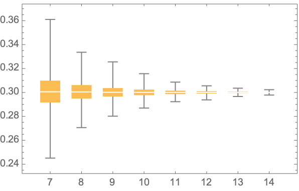
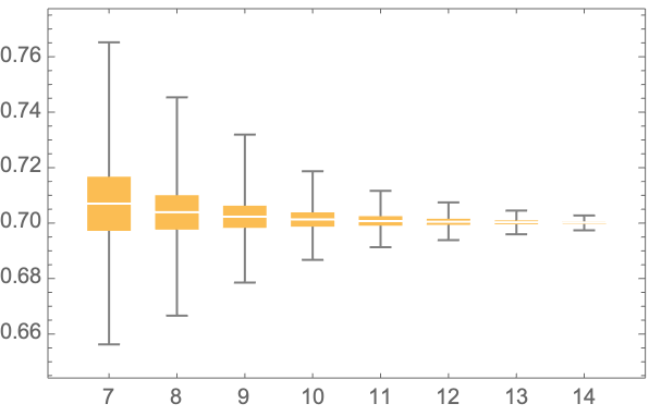
Figure 1: Box plots of $\widehat{R}_{n}$ for $n=7,\dots,14$ based on 10,000 sample paths of fractional Brownian motion with $R=0.3$ (left) and $R=0.7$ (right).

But the estimator $\widehat{R}_{n}$ also has a disadvantage: it is not scale-invariant. Indeed, we clearly have

$$\widehat{R}_{n}(\lambda x)-\widehat{R}_{n}(x)=-\frac{\log_{2}|\lambda|}{n}\qquad\text{for $\lambda\neq 0$.}$$ (8.1)

As a consequence, multiplying $x$ with a constant factor can lead to negative or unreasonably large estimates for $R$ and substantially slow down or speed up the convergence $\widehat{R}_{n}(x)\to R$ (note that both the roughness exponent itself and the reverse Jensen condition are scale-invariant). Naive normalization of the data does not provide a resolution of this issue, as is illustrated in Figure 2. In the next subsection, we are therefore going to derive intrinsically defined optimal scaling factors and the corresponding improved estimators for the roughness exponent.

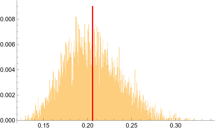
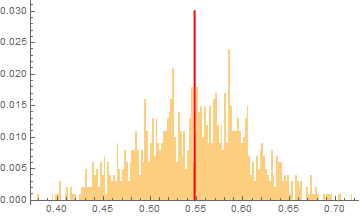
Figure 2: Histograms of $\widehat{R}_{12}$ applied to 5000 standardized sample paths of fractional Brownian motion with Hurst parameters $H=0.3$ (left) and $H=0.7$ (right). Here, standardization means that each sample path is affinely scaled to have empirical mean zero and variance one. The red vertical lines represent the empirical means of the corresponding estimates.

When presented with a generic time series, we face significant uncertainty about possible data scaling that, as discussed above, can lead to significant underperformance of the estimator $\widehat{R}_{n}$. In this section, we will therefore analyze two ideas on constructing scale-invariant estimators for the roughness exponent out of the sequence $(\widehat{R}_{n})$. Both ideas will lead to new estimators that are linear combinations of $\widehat{R}_{n},\dots,\widehat{R}_{n-m}$ for a number $m$.

The first idea consists in looking for a scaling factor $\lambda_{n}$ that optimizes a certain criterion over all possible parameters $\lambda>0$ and then to take $\widehat{R}_{n}(\lambda_{n}x)$ as a new estimator. In particular, we will look at the following two choices. A third choice will be given in Definition 8.2.

Definition 8.1.

Fix $m\in\mathbb{N}$ and $\alpha_{0},\dots,\alpha_{m}\geq 0$ with $\alpha_{0}>0$.

1. For $n>m$, the sequential scaling factor $\lambda_{n}^{s}$ and the sequential scale estimate $R^{s}_{n}(x)$ are defined as follows,

   $$\begin{split}\lambda^{s}_{n}&:=\mathop{\hbox{\rm arg\,min}}_{\lambda>0}\sum_{k=n-m}^{n}\alpha_{n-k}\Big{(}\widehat{R}_{k}(\lambda x)-\widehat{R}_{k-1}(\lambda x)\Big{)}^{2}\quad\text{and}\quad R^{s}_{n}(x):=\widehat{R}_{n}(\lambda^{s}_{n}x).\end{split}$$ (8.2)

   The corresponding mapping $R^{s}_{n}:C[0,1]\rightarrow{\mathbb{R}}$ will be called the sequential scale estimator.

2. The terminal scaling factor $\lambda_{n}^{t}$ and the terminal scale estimate $R_{n}^{t}(x)$ are defined as follows,

   $$\begin{split}\lambda^{t}_{n}&:=\mathop{\hbox{\rm arg\,min}}_{\lambda>0}\sum_{k=n-m}^{n}\alpha_{n-k}\Big{(}\widehat{R}_{n}(\lambda x)-\widehat{R}_{k-1}(\lambda x)\Big{)}^{2}\quad\text{and}\quad R_{n}^{t}(x):=\widehat{R}_{n}(\lambda^{t}_{n}x).\end{split}$$ (8.3)

   The corresponding mapping $R_{n}^{t}:C[0,1]\rightarrow{\mathbb{R}}$ will be called the terminal scale estimator.

We will see in Proposition 8.3 that Definition 8.1 is well posed, because the minimization problems in (8.2) and (8.3) admit unique solutions for every function $x\in C[0,1]$. The intuition for sequential scaling is fairly simple. The sequential scaling factor $\lambda^{s}_{n}$ minimizes the weighted mean-squared differences $\widehat{R}_{k}(\lambda x)-\widehat{R}_{k-1}(\lambda x)$ for $k=m+1,\dots,n$. Since $\widehat{R}_{n}$ is a consistent estimator, the faster the sequence $\widehat{R}_{k}(\lambda x)$ converges, the more accurate the final estimate $\widehat{R}_{n}(\lambda x)$ will be. The idea for terminal scaling is also straightforward: Since the estimator $\widehat{R}_{n}$ is consistent, the last estimate $\widehat{R}_{n}(x)$ should be more precise than any other previous value $\widehat{R}_{k}(x)$ with $k<n$. Therefore, we aim at minimizing the weighted mean-squared differences $\widehat{R}_{k}(\lambda x)$ and $\widehat{R}_{n}(\lambda x)$.

Our second idea for constructing a scale-invariant estimator is as follows. It follows from (8.1) that for $\lambda>0$

$$n\widehat{R}_{n}(x)=n\widehat{R}_{n}(\lambda x)+\log_{2}\lambda.$$

For an ideal scaling factor $\lambda$, the right-hand side will be close to $nR+\log_{2}|\lambda|$. Therefore, the idea is to perform linear regression on the data points $(n-m)\widehat{R}_{n-m}(x),(n-m-1)\widehat{R}_{n-m-1}(x),\dots,n\widehat{R}_{n}(x)$ and to take the corresponding slope as an estimator for $R$.

Definition 8.2.

Let $m\in\mathbb{N}$ and $\alpha_{0},\dots,\alpha_{m}\geq 0$ be such that $\sum_{k=0}^{m}\alpha_{k}=1$. Then, for $n>m$, the regression scale estimate $R^{r}_{n}(x)$ and the regression scaling factor $\lambda^{r}_{n}$ are given by

$$(R^{r}_{n}(x),\lambda^{r}_{n})=\mathop{\hbox{\rm arg\,min}}_{h\in{\mathbb{R}},\,\lambda>0}\sum_{k=0}^{m}\alpha_{k}\Big{(}(n-k)(\widehat{R}_{n-k}(x)-h)-\log_{2}\lambda\Big{)}^{2}.$$ (8.4)

The corresponding mapping $R_{n}^{r}:C[0,1]\rightarrow{\mathbb{R}}$ will be called the regression scale estimator.

The next proposition shows in particular that all three estimators can be represented by linear combinations of the estimators $\widehat{R}_{k}$ for $m\leq k\leq n$ and that they are scale-invariant estimators of the roughness exponent $R$.

Proposition 8.3.

Consider the context of Definitions 8.1 and 8.2 with fixed $m\in\mathbb{N}$ and $\alpha_{0},\dots,\alpha_{m}\geq 0$ such that $\alpha_{0}>0$.

1. The three optimization problems in (8.2), (8.3), and (8.4) admit unique solutions for every function $x\in C[0,1]$. In particular, all objects in Definitions 8.1 and 8.2 are well defined.

2. The sequential and terminal scale estimators can be represented by the following respective linear combinations of the estimators $\widehat{R}_{k}$,

   $$R^{s}_{n}=\beta_{n,n}\widehat{R}_{n}+\cdots+\beta_{n,n-m-1}\widehat{R}_{n-m-1}\qquad\text{and}\qquad R^{t}_{n}=\gamma_{n,n}\widehat{R}_{n}+\cdots+\gamma_{n,n-m-1}\widehat{R}_{n-m-1}$$

   where

   $$\beta_{n,k}=\begin{cases}\displaystyle 1+\frac{\alpha_{0}}{c^{\textrm{\rm s}}_{n}n^{2}(n-1)}&\text{if $k=n$,}\\ \displaystyle\frac{1}{c^{\textrm{\rm s}}_{n}nk}\Big{(}\frac{\alpha_{n-k}}{k-1}-\frac{\alpha_{n-k-1}}{k+1}\Big{)}&\text{if $n-m\leq k\leq n-1$,}\\ \displaystyle\frac{-\alpha_{m}}{c^{\textrm{\rm s}}_{n}n(n-m)(n-m-1)}&\text{if $k=n-m-1$,}\end{cases}\quad\text{for}\quad c^{s}_{n}:=\sum_{k=n-m}^{n}\frac{\alpha_{n-k}}{k^{2}(k-1)^{2}},$$

   and

   $$\gamma_{n,k}=\begin{cases}\displaystyle 1+\frac{1}{c_{n}^{t}n^{2}}\sum_{j=n-m}^{n}\alpha_{n-j}\frac{n-j+1}{j-1}&\text{if $k=n$,}\\ \displaystyle\frac{k-n}{c_{n}^{t}n^{2}k}\alpha_{n-k-1}&\text{otherwise,}\end{cases}\quad\text{for}\quad c_{n}^{t}=\sum_{k=n-m}^{n}\alpha_{n-k}\Big{(}\frac{n-k+1}{n(k-1)}\Big{)}^{2}.$$

   If in addition $\sum_{k}\alpha_{k}=1$, then the regression scale estimator is given by

   $$\begin{split}R^{r}_{n}=\frac{1}{c^{r}}\sum_{k=0}^{m}\alpha_{k}(n-k)\big{(}k-a)\widehat{R}_{n-k},\qquad\text{where $\displaystyle a=\sum_{k=0}^{m}\alpha_{k}k$ and $\displaystyle c^{r}=a^{2}-\sum_{k=0}^{m}\alpha_{k}k^{2}$.}\end{split}$$ (8.5)

3. The sequential, terminal, and regression scale estimators are scale-invariant. That is, for $n>m$, $x\in C[0,1]$, and $\lambda\neq 0$, we have $R^{t}_{n}(\lambda x)=R^{t}_{n}(x)$, $R^{s}_{n}(\lambda x)=R^{s}_{n}(x)$ and $R^{r}_{n}(\lambda x)=R^{r}_{n}(x)$.

4. If $x\in C[0,1]$ is such that there exists $\lambda\neq 0$ for which $|\widehat{R}_{n}(\lambda x)-R|=O(a_{n})$ as $n\uparrow\infty$ for some sequence $(a_{n})$ with $a_{n}=o(1/n)$, then $|R^{s}_{n}(x)-R|$, $|R^{t}_{n}(x)-R|$, and $|R^{r}_{n}(x)-R|$ are all of the order $O(na_{n})$.

Proof.

We prove (a) and (b) together. Fix $x\in C[0,1]$. For $\lambda>0$ we write $\phi:=\log_{2}\lambda$ and we will minimize (8.2) and (8.3) over $\phi$ rather than over $\lambda$. Recall from (8.1) that

$$\widehat{R}_{k}(2^{\phi}x)=\widehat{R}_{k}(x)-\frac{\phi}{k}.$$ (8.6)

One therefore sees that the objective functions in (8.2) and (8.3) are strictly convex in $\phi$, and so minimizers can be computed as the unique zeros of the corresponding derivatives. Differentiating the objective function in (8.2) and summing by parts gives

$$\frac{1}{2}\frac{\partial}{\partial\phi}\sum_{k=n-m}^{n}\alpha_{n-k}\Big{(}\widehat{R}_{k}(2^{\phi}x)-\widehat{R}_{k-1}(2^{\phi}x)\Big{)}^{2}$$

$$=c^{s}_{n}\phi+\frac{\alpha_{0}\widehat{R}_{n}(x)}{n(n-1)}+\sum_{k=n-m}^{n-1}\widehat{R}_{k}(x)\Big{(}\frac{\alpha_{n-k}}{k(k-1)}-\frac{\alpha_{n-k-1}}{(k+1)k}\Big{)}-\frac{\alpha_{m}\widehat{R}_{n-m-1}(x)}{(n-m)(n-m-1)}.$$ (8.7)

Setting this expression equal to zero yields the global minimizer $\phi^{s}_{n}$,

$$\phi^{s}_{n}=-\frac{1}{c^{s}_{n}}\bigg{(}\frac{\widehat{R}_{n}(x)}{n}\cdot\frac{\alpha_{0}}{n-1}+\sum_{k=n-m}^{n-1}\frac{\widehat{R}_{k}(x)}{k}\Big{(}\frac{\alpha_{n-k}}{k-1}-\frac{\alpha_{n-k-1}}{k+1}\Big{)}-\frac{\widehat{R}_{n-m-1}(x)}{n-m-1}\cdot\frac{\alpha_{m}}{n-m}\bigg{)}.$$

Applying (8.6) to $\widehat{R}_{n}(2^{\phi_{n}^{s}}x)$ yields the asserted expression for the sequential scale estimator. The proof for the terminal scale estimator is analogous. The assertion for the regression scale estimator follows by standard computations for linear regression.

(c) For $\eta>0$, we have

$$\mathop{\hbox{\rm arg\,min}}_{\lambda>0}\sum_{k=n-m}^{n}\alpha_{n-k}\Big{(}\widehat{R}_{k}(\lambda\eta x)-\widehat{R}_{k-1}(\lambda\eta x)\Big{)}^{2}=\frac{1}{\eta}\mathop{\hbox{\rm arg\,min}}_{\lambda>0}\sum_{k=n-m}^{n}\alpha_{n-k}\Big{(}\widehat{R}_{k}(\lambda x)-\widehat{R}_{k-1}(\lambda x)\Big{)}^{2}=\frac{\lambda^{s}_{n}}{\eta},$$

where $\lambda^{s}_{n}$ is the sequential scaling factor. Therefore, $R^{s}_{n}(\eta x)=\widehat{R}_{n}(\lambda^{s}_{n}x)=R^{s}_{n}(x)$. The same argument yields the scale invariance of the terminal and regression scale estimators.

(d) Clearly, we can assume without loss of generality that $\lambda=1$. First, we consider the sequential scale estimator. Using (8.7) one sees that $\sum_{k}\beta_{n,k}=1$ so that

$$R^{s}_{n}-R=\beta_{n,n}(\widehat{R}_{n}-R)+\cdots+\beta_{n,n-m-1}(\widehat{R}_{n-m-1}-R).$$

Since $\beta_{n,n-k}=O(n)$ for each $k$, the assertion follows. The proof for the terminal scale estimator is analogous. For the regression scale estimator, one checks that $\frac{1}{c^{r}}\sum_{k=0}^{m}\alpha_{k}(n-k)\big{(}k-a)=1$ and proceeds as before. ∎

Part (d) of Proposition 8.3 implies in particular the consistency of the sequential, terminal, and regression scale estimators if $x\in C[0,1]$ satisfies $|\widehat{R}_{n}(\lambda x)-R|=o(1/n)$ for some $\lambda\neq 0$. It also enables us to obtain the convergence rate of the estimators $R^{s}_{n}$, $R^{t}_{n}$ and $R^{r}_{n}$ for the sample paths of fractional Brownian motion with drift.

Corollary 8.4.

Let $X^{H}$ be a fractional Brownian motion with drift as in (5.1). Then the following almost sure rates of convergence hold for the scale-invariant estimator $R_{n}^{p}$ with $p\in\{s,t,r\}$,

$$\left|R^{p}_{n}(X^{H})-H\right|=\begin{cases}O\left(2^{-n/2}\sqrt{\log n}\right)&\text{if $H\in(0,\frac{1}{2})$,}\\ O\left(2^{-n/2}n^{1/2}\sqrt{\log n}\right)&\text{if $H=\frac{1}{2}$,}\\ O\left(2^{(H-1)n}\sqrt{\log n}\right)&\text{if $H\in(\frac{1}{2},1)$.}\end{cases}$$ (8.8)

Remark 8.5.

A general scale-invariant estimator $\widetilde{R}_{n}$ can be constructed by solving an optimization problem of the form

$$\widetilde{\lambda}:=\mathop{\hbox{\rm arg\,min}}_{\lambda>0}\sum_{j>k}^{n}\alpha_{j,k}|\widehat{R}_{j}(\lambda x)-\widehat{R}_{k}(\lambda x)|^{2},$$

where $\alpha_{j,k}$ are given coefficients, and by setting $\widetilde{R}_{n}(x):=\widehat{R}_{n}(\widetilde{\lambda}x)$. If the global minimizer $\widetilde{\lambda}$ exists, the estimate $\widetilde{R}_{n}(x)$ will be a linear combination of the estimates $\widehat{R}_{k}(x)$.

Let us now investigate the relations between our estimators and the one used in [13]. To this end, we let for $x\in C[0,1]$, $n,k\in\mathbb{N}$ and $q\in{\mathbb{R}}^{-}$,

$$m(q,k,n):=\Big{\lfloor}{\frac{k}{2^{n}}}\Big{\rfloor}^{-1}\sum_{j=1}^{\lfloor 2^{n}/k\rfloor}|x(kj2^{-n})-x(k(j-1)2^{-n})|^{q}.$$

Following Rosenbaum [32], Gatheral et al. [13] assume that there exists a positive constant $b_{q}$ such that

$$\big{(}k2^{-n}\big{)}^{-qR}m(q,k,n)\rightarrow b_{q},\qquad\text{for any fixed $k\in\mathbb{N}$, as $n\uparrow\infty$,}$$

From here, the estimator $R_{n}^{v}$ from [13] is computed by way of a linear regression. More precisely, let $\mathcal{K}$ be a finite collection of positive integers and $\mathcal{Q}$ be a finite collection of positive real numbers. For $q\in\mathcal{Q}$, the estimate $R_{n,q}^{v}(x)$ of the roughness exponent of the continuous function $x$ using the $q^{\text{th}}$ variation is obtained by regressing $\log_{2}m(q,k,n)$ with respect to $\log_{2}k$, i.e.,

$$(R_{n,q}^{v}(x),b_{q})=\mathop{\hbox{\rm arg\,min}}_{h\in{\mathbb{R}},\,b_{q}>0}\sum_{k\in\mathcal{K}}\Big{(}\log_{2}m(q,k,n)-\log_{2}b_{q}-qh(\log_{2}k-n)\Big{)}^{2}.$$ (8.9)

Standard computations for linear regression then yield that

$$R_{n,q}^{v}(x)=\dfrac{\sum_{k\in\mathcal{K}}\big{(}\log_{2}k-\overline{\log_{2}\mathcal{K}}\big{)}\big{(}\log_{2}m(q,k,n)-\overline{\log_{2}m(q,\mathcal{K},n)}\big{)}}{q\cdot\sum_{k\in\mathcal{K}}\big{(}\log_{2}k-\overline{\log_{2}\mathcal{K}}\big{)}},$$

where $|\cdot|$ denotes the cardinality of a set and

$$\overline{\log_{2}\mathcal{K}}=\frac{1}{|\mathcal{K}|}\sum_{k\in\mathcal{K}}\log_{2}k\quad\text{and}\quad\overline{\log_{2}m(q,\mathcal{K},n)}=\frac{1}{|\mathcal{K}|}\sum_{k\in\mathcal{K}}\log_{2}m(q,k,n).$$

The simple regression estimate $R_{n}^{v}(x)$ is then the sample average of $R_{n,q}^{v}(x)$ for all $q\in\mathcal{Q}$. In other words, we have

$$R_{n}^{v}(x):=\frac{1}{|\mathcal{Q}|}\sum_{q\in\mathcal{Q}}R_{n,q}^{v}(x).$$

The corresponding mapping $R_{n}^{v}:C[0,1]\rightarrow{\mathbb{R}}$ will be called the simple regression estimator, which is a formal description of the estimator used in [13]. It is also clear that the simple regression estimator $R^{v}_{n}$ is scale-invariant, i.e., for any $n\in\mathbb{N}$ and $x\in C[0,1]$, we have $R^{v}_{n}(\lambda x)=R^{v}_{n}(x)$ for any $\lambda\neq 0$. Our next result states that the simple regression estimator is a particular case of our regression scale estimator under a certain choice of parameters.

Proposition 8.6.

Let $\mathcal{Q}=\{2\}$, $\mathcal{K}=\{1,2,\cdots,2^{m}\}$ and $\alpha_{k}=\alpha$ for all $k$ and some $\alpha>0$. Then the regression scale estimator $R^{r}_{n}$ coincides with the simple regression estimator $R^{v}_{n}$ for all $n>m$.

Proof.

Since the minimization problems in (8.4) and (8.9) admit unique solutions for every function $x\in C[0,1]$, it suffices to show (8.4) is equivalent to (8.9) when taking the above parameters. Let $\lambda=1/\sqrt{b_{2}}$, and we rewrite optimization problem in (8.9) into

$$\begin{split}&\mathop{\hbox{\rm arg\,min}}_{h\in{\mathbb{R}},\,b_{q}>0}\sum_{k\in\mathcal{K}}\Big{(}\log_{2}m(2,k,n)-\log_{2}b_{2}-2h(\log_{2}k-n)\Big{)}^{2}\\ &=\mathop{\hbox{\rm arg\,min}}_{h\in{\mathbb{R}},\,\lambda>0}\sum_{j=0}^{m}\Big{(}2(j-n)+2\log_{2}s_{n-j}+2\log_{2}\lambda-2h(j-n)\Big{)}^{2}\\ &=\mathop{\hbox{\rm arg\,min}}_{h\in{\mathbb{R}},\,b_{q}>0}\sum_{j=0}^{m}\alpha\cdot\Big{(}(n-j)(\widehat{R}_{n-j}(x)-h)-\log_{2}\lambda\Big{)}^{2},\end{split}$$

where the second identity follows from [28, Proposition 2.1].∎

9 The roughness exponent for unequally spaced partitions

In this section, we will relax our assumption that the data points for sampling the $p^{\text{th}}$ variation $\langle x\rangle_{n}^{(p)}$ of $x$ are located at the $n^{\text{th}}$ dyadic partition of the time interval $[0,1]$. To this end, let us first recall that a partition of the interval $[0,1]$ is a finite set $\mathbb{T}=\{t_{0},\dots,t_{m}\}$ such that $0=t_{0}<t_{1}<\cdots<t_{m}=1$. Its mesh is defined as the maximal distance between two neighboring partition points. A sequence $(\mathbb{T}_{n})_{n\in\mathbb{N}_{0}}$ of partitions of $[0,1]$ is called a refining sequence of partitions of $[0,1]$ if $\mathbb{T}_{0}\subset\mathbb{T}_{1}\subset\cdots$ and the mesh of $\mathbb{T}_{n}$ tends to $0$ as $n\uparrow\infty$. In this case, we will generically write $\mathbb{T}_{n}=\{t_{0}^{n},t^{n}_{1},\dots,t_{m_{n}}^{n}\}$. For simplicity, we will henceforth assume that $\mathbb{T}_{0}=\{0,1\}$ and that, when passing from $\mathbb{T}_{n}$ to $\mathbb{T}_{n+1}$, exactly one new partition point is added between any two neighboring partition points of $\mathbb{T}_{n}$, i.e., $|(t_{k-1}^{n},t^{n}_{k})\cap\mathbb{T}_{n+1}|=1$. This assumption can always be satisfied by re-arranging the partitions, and in this case, we have $m_{n}=2^{n}$. Furthermore, under this assumption, it follows $t^{n}_{k}=t^{n+1}_{2k}$.

In Section 2, the definition of the roughness exponent of a continuous function $x$ was based on the Faber–Schauder expansion of $x$. The Faber–Schauder functions are clearly tied to the sequence of dyadic partitions, but, similar to Cont and Das [5], the definition of the Faber–Schauder functions can be extended to our present setup as follows. First, let $b_{\emptyset}(t):=t$. Next, for $n\in\mathbb{N}_{0}$ and $k\in\{0,\dots,2^{n}-1\}$, we define

$$b_{n,k}(t):=\begin{cases}\displaystyle\frac{t-t^{n+1}_{2k}}{t^{n+1}_{2k+1}-t^{n+1}_{2k}}&\text{if $t\in[t^{n+1}_{2k},t^{n+1}_{2k+1})$,}\\ &\\ \displaystyle\frac{t^{n+1}_{2k+2}-t}{t^{n+1}_{2k+2}-t^{n+1}_{2k+1}}&\text{if $t\in[t^{n+1}_{2k+1},t^{n+1}_{2k+2})$,}\\ &\\ 0&\text{otherwise.}\end{cases}$$

It is shown in [5, Section 3.3] that any function $x\in C[0,1]$ can by represented by the following uniformly convergent series,

$${x}(t)={f}(0)+(x(1)-x(0))t+\sum_{m=0}^{\infty}\sum_{k=0}^{2^{m}-1}\theta_{m,k}b_{m,k}(t),\qquad t\in[0,1],$$ (9.1)

where

$$\theta_{n,k}:=x(t^{n+1}_{2k+1})-\frac{t^{n+1}_{2k+2}-t^{n+1}_{2k+1}}{t^{n+1}_{2k+2}-t^{n+1}_{2k}}x(t^{n+1}_{2k})-\frac{t^{n+1}_{2k+1}-t^{n+1}_{2k}}{t^{n+1}_{2k+2}-t^{n+1}_{2k}}x(t^{n+1}_{2k+2})$$ (9.2)

will be called the generalized Faber–Schauder coefficients of $x$. For $p>0$ and $n\in\mathbb{N}$, we define the $p^{\text{th}}$ variation of the function $x$ along $\mathbb{T}_{n}$ by

$$\langle x\rangle_{n}^{(p)}:=\sum_{k=0}^{2^{n}-1}\big{|}x(t^{n}_{k+1})-x(t^{n}_{k})\big{|}^{p}.$$

If there exists $q\in[1,\infty]$ such that

$$\lim\limits_{n\uparrow\infty}\langle x\rangle_{n}^{(p)}=\begin{cases}0&\quad p>q,\\ \infty&\quad p<q,\end{cases}$$

the roughness exponent of $x$ (with respect to $(\mathbb{T}_{n})_{n\in\mathbb{N}_{0}}$) is defined as $R=1/q$. The following definition formulates the reverse Jensen condition for the irregular Faber–Schauder coefficients defined in (9.2).

Definition 9.1.

We say that the coefficients $(\theta_{m,k})$ of $x$ satisfy the reverse Jensen condition if for each $p\geq 1$, there exists a non-decreasing subexponential function $\varrho_{p}:\mathbb{N}\rightarrow[1,\infty)$ such that

$$\begin{split}\frac{1}{\varrho_{p}(n)}\Big{(}\sum_{m=0}^{n-1}\sum_{k=0}^{2^{m-1}-1}&\frac{\theta_{m,k}^{2}}{t^{m}_{2k+1}-t^{m}_{2k}}+\frac{\theta_{m,k}^{2}}{t^{m}_{2k+2}-t^{m}_{2k+1}}\Big{)}^{p/2}\leq\Big{(}\sum_{k=0}^{2^{n}-1}\sum_{m=0}^{n-1}\frac{\theta^{2}_{m,\lfloor 2^{m-n+1}k\rfloor}}{t^{m}_{\lfloor 2^{m-n}k\rfloor+1}-t^{m}_{\lfloor 2^{m-n}k\rfloor}}\Big{)}^{p/2}\\ &\leq\varrho_{p}(n)\Big{(}\sum_{m=0}^{n-1}\sum_{k=0}^{2^{m-1}-1}\frac{\theta_{m,k}^{2}}{t^{m}_{2k+1}-t^{m}_{2k}}+\frac{\theta_{m,k}^{2}}{t^{m}_{2k+2}-t^{m}_{2k+1}}\Big{)}^{p/2}\quad\text{for }n\in\mathbb{N}.\end{split}$$

To formulate our extension of Theorem 2.4 to unequally spaced partitions, we need an additional condition on our partitions sequence. Let us denote

$$\overline{\pi}_{n}:=\sup_{k}|t^{n}_{k+1}-t^{n}_{k}|\quad\text{and}\quad\underline{\pi}_{n}:=\inf_{k}|t^{n}_{k+1}-t^{n}_{k}|.$$

We will say that the sequence $(\mathbb{T}_{n})_{n\in\mathbb{N}_{0}}$ is well-balanced if there exists a non-decreasing subexponential function $\kappa$ such that

$$\sup_{k\leq n}\frac{\overline{\pi}_{k}}{\underline{\pi}_{k}}\leq\kappa(n),\qquad n\in\mathbb{N}_{0}.$$

The similar, but slightly different concept of a balanced partition sequence was introduced earlier by Cont and Das [6, 5]. Furthermore, for $n\in\mathbb{N}$, we now denote likewise

$$s_{n}:=\sqrt{\sum_{m=0}^{n-1}\sum_{k=0}^{2^{m}-1}2^{m}\theta^{2}_{m,k}}\quad\text{and}\quad\widehat{R}_{n}(x)=1-\frac{1}{n}\log_{2}s_{n}.$$

The next theorem shows that the roughness exponent defined over a sequence of well-balanced partitions, its value can be obtained from the sequence $(s_{n})_{n\in\mathbb{N}}$.

Theorem 9.2.

Suppose that the generalized Faber–Schauder coefficients of $x$ satisfy the reverse Jensen condition and the partition sequence $(\mathbb{T}_{n})_{n\in\mathbb{N}_{0}}$ is well-balanced. Then the function $x$ admits the roughness exponent $R$ if and only if the finite limit $r:=\lim_{n}\widehat{R}_{n}(x)$ exists, and in that case we have $R=r$.

Before proving Theorem 9.2, let us show that the main result of dyadic partitions can been directly recovered from Theorem 9.2. Suppose $(\mathbb{T}_{n})_{n\in\mathbb{N}_{0}}$ is the sequence of dyadic partitions and the function $x\in C[0,1]$ admits the Faber–Schauder coefficients $(\mu_{m,k})$. Then it follows that

$$\mu_{m,k}=2^{m/2+1}\theta_{m,k}\quad\text{and}\quad s_{n}=\sqrt{\frac{1}{2}\sum_{m=0}^{n-1}\sum_{k=0}^{2^{m}-1}\mu_{m,k}^{2}},$$

which then reproduces Theorem 2.4. To prepare for the proof of Theorem 9.2, we define for $n\in\mathbb{N}$,

$$V_{n}:=\sum_{k=0}^{2^{n}-1}\bigg{(}\frac{1}{t^{n+1}_{2k+1}-t^{n+1}_{2k}}{\mathbbmss{1}}_{{}_{\scriptstyle[t^{n+1}_{2k},t^{n+1}_{2k+1})}}-\frac{1}{t^{n+1}_{2k+2}-t^{n+1}_{2k+1}}{\mathbbmss{1}}_{{}_{\scriptstyle[t^{n+1}_{2k+1},t^{n+1}_{2k+2})}}\bigg{)}.$$ (9.3)

Then $V_{n}$ is equal to the right-hand derivative of the function $\sum_{k=0}^{2^{n}-1}b_{n,k}$. We consider each $V_{n}$ as a random variable on the probability space $([0,1],{\mathscr{F}},{\mathbb{P}})$, where ${\mathscr{F}}$ is the Borel $\sigma$-field of $[0,1]$ and ${\mathbb{P}}$ is the Lebesgue measure on ${\mathscr{F}}$. When defining the $\sigma$-field

$${\mathscr{F}}_{n}:=\sigma\big{(}[t^{n}_{k},t^{n}_{k+1}):k=0,\dots,2^{n}-1\big{)},$$

one sees that $V_{n}$ is ${\mathscr{F}}_{n+1}$-measurable. Let us moreover define random variables $\vartheta_{n}:[0,1]\to{\mathbb{R}}$ by

$$\vartheta_{n}:=\sum_{k=0}^{2^{n}-1}\theta_{n,k}{\mathbbmss{1}}_{{}_{\scriptstyle[t^{n}_{k},t^{n}_{k+1})}}.$$ (9.4)

Clearly, the random variable $\vartheta_{n}$ is ${\mathscr{F}}_{n}$–measurable. For each $n\in\mathbb{N}$, let $x_{n}$ denote the $n^{\text{th}}$ truncation of $x$, defined in analogy to (3.10). Then

$$x_{n}(t)=\int_{0}^{t}\sum_{m=0}^{n-1}\vartheta_{m}(s)V_{m}(s)\,ds.$$

Since $\vartheta_{m}$ and $V_{m}$ are constant on intervals of the form $[t^{n}_{k},t^{n}_{k+1})$ for $n\geq m$, we have

$$x(t^{n}_{k+1})-x(t^{n}_{k})=x_{n}(t^{n}_{k+1})-x_{n}(t^{n}_{k})=(t^{n}_{k+1}-t^{n}_{k})\sum_{m=0}^{n-1}\vartheta_{m}(t)V_{m}(t).$$ (9.5)

Hence, for $p\geq 1$,

$$\langle x\rangle_{n}^{(p)} =\sum_{k=0}^{2^{n}-1}\big{|}x(t^{n}_{k+1})-x(t^{n}_{k})\big{|}^{p}=\sum_{k=0}^{2^{n}-1}\bigg{|}(t^{n}_{k+1}-t^{n}_{k})\sum_{m=1}^{n}\vartheta_{m}(t^{n}_{k})V_{m}(t^{n}_{k})\bigg{|}^{p}$$

$$=\sum_{k=0}^{2^{n}-1}(t^{n}_{k+1}-t^{n}_{k})\cdot\bigg{|}\gamma_{n,p}(t_{k})\sum_{m=0}^{n-1}\vartheta_{m}(t_{k})V_{m}(t_{k})\bigg{|}^{p}={\mathbb{E}}\bigg{[}\bigg{|}\gamma_{n,p}\sum_{m=0}^{n-1}\vartheta_{m}V_{m}\bigg{|}^{p}\bigg{]},$$

where the expectation is taken under the Lebesgue measure ${\mathbb{P}}$ and

$$\gamma_{n,p}(t):=\sum_{k=0}^{2^{n}-1}(t^{n}_{k+1}-t^{n}_{k})^{\frac{p-1}{p}}{\mathbbmss{1}}_{{}_{\scriptstyle[t^{n}_{k+1},t^{n}_{k})}}(t).$$

By definition, $\gamma_{n,p}$ is constant on all intervals of the form $[t^{n}_{k},t^{n}_{k+1})$ and hence ${\mathscr{F}}_{n}$-measurable. Moreover, Hölder’s inequality yields that

$${\mathbb{E}}[\gamma_{n,p}^{-p}]^{-1}\cdot{\mathbb{E}}\bigg{[}\bigg{|}\sum_{m=0}^{n-1}\vartheta_{m}V_{m}\bigg{|}^{p/2}\bigg{]}^{2}\leq{\mathbb{E}}\bigg{[}\bigg{|}\gamma_{n,p}\sum_{m=0}^{n-1}\vartheta_{m}V_{m}\bigg{|}^{p}\bigg{]}\leq{\mathbb{E}}[\gamma_{n,p}^{2p}]^{1/2}\cdot{\mathbb{E}}\bigg{[}\bigg{|}\sum_{m=0}^{n-1}\vartheta_{m}V_{m}\bigg{|}^{2p}\bigg{]}^{1/2}.$$ (9.6)

Now take $M_{0}:=0$ and

$$M_{n}:=\sum_{m=0}^{n-1}\vartheta_{m}V_{m}=\sum_{m=0}^{n-1}\vartheta_{m}(N_{m+1}-N_{m}),\qquad n=1,2,\dots.$$

Since for each $m$, the random variable $\vartheta_{m}$ is bounded and ${\mathscr{F}}_{m}$-measurable, $(M_{n})_{n=0,1,\dots}$ is a martingale transform of the martingale $(N_{n})_{n=0,1,\dots}$ and hence itself a martingale. We first compute the expectations of the random variable $\gamma_{n,p}$ occurring on both bounds,

$$\begin{split}{\mathbb{E}}[\gamma_{n,p}^{2p}]^{1/2}&=\Big{(}\sum_{k=0}^{2^{n}-1}(t^{n}_{k+1}-t^{n}_{k})^{2(p-1)}\cdot(t^{n}_{k+1}-t^{n}_{k})\Big{)}^{1/2}=\Big{(}\sum_{k=0}^{2^{n}-1}(t^{n}_{k+1}-t^{n}_{k})^{2p-1}\Big{)}^{1/2}.\\ {\mathbb{E}}[\gamma_{n,p}^{-p}]^{-1}&=\Big{(}\sum_{k=0}^{2^{n}-1}(t^{n}_{k+1}-t^{n}_{k})^{-(p-1)}\cdot(t^{n}_{k+1}-t^{n}_{k})\Big{)}^{-1}=\Big{(}\sum_{k=0}^{2^{n}-1}(t^{n}_{k+1}-t^{n}_{k})^{2-p}\Big{)}^{-1}.\end{split}$$

Furthermore, the Burkholder inequality yields constants $0<A_{p}\leq B_{p}<\infty$, depending only on $p$ but not on $x$, such that

$$A_{p}{\mathbb{E}}\big{[}[M]_{n}^{p}\big{]}\leq{\mathbb{E}}\Big{[}\big{|}M_{n}\big{|}^{2p}\Big{]}\leq B_{p}{\mathbb{E}}\big{[}[M]_{n}^{p}\big{]},$$

where

$$[M]_{n}=\sum_{m=1}^{n}(M_{m}-M_{m-1})^{2}=\sum_{m=0}^{n-1}\vartheta^{2}_{m}V^{2}_{m}.$$

Note that we can also rephrase the reverse Jensen condition in Definition 9.1 in the same way as in (3.6):

$$\frac{1}{\varrho_{p}(n)}{\mathbb{E}}\big{[}\sum_{m=0}^{n-1}V^{2}_{m}\vartheta^{2}_{m}\big{]}^{p/2}\leq{\mathbb{E}}\big{[}\Big{(}\sum_{m=0}^{n-1}V^{2}_{m}\vartheta^{2}_{m}\Big{)}^{p/2}\big{]}\leq\varrho_{p}(n){\mathbb{E}}\big{[}\sum_{m=0}^{n-1}V^{2}_{m}\vartheta^{2}_{m}\big{]}^{p/2}.$$

It then follows from the reverse Jensen condition that

$$\frac{1}{\varrho_{p}(n)}{\mathbb{E}}\big{[}[M]_{n}\big{]}^{p}\leq{\mathbb{E}}\big{[}[M]_{n}^{p}\big{]}\leq\varrho_{p}(n){\mathbb{E}}\big{[}[M]_{n}\big{]}^{p}.$$

Now, we get

$${\mathbb{E}}\big{[}[M]_{n}\big{]}={\mathbb{E}}\big{[}\sum_{m=0}^{n-1}\vartheta^{2}_{m}V^{2}_{m}\big{]}=\sum_{m=0}^{n-1}\sum_{k=0}^{2^{m}-1}\frac{\theta_{m,k}^{2}}{t^{m+1}_{2k+1}-t^{m+1}_{2k}}+\frac{\theta_{m,k}^{2}}{t^{m+1}_{2k+2}-t^{m+1}_{2k+1}}$$

Combining the previous inequalities and the above equality yields

$$\langle x\rangle_{n}^{(p)}\leq C_{p}\varrho_{p}(n)\Big{(}\sum_{m=0}^{n-1}\sum_{k=0}^{2^{m}-1}\frac{\theta_{m,k}^{2}}{t^{m+1}_{2k+1}-t^{m+1}_{2k}}+\frac{\theta_{m,k}^{2}}{t^{m+1}_{2k+2}-t^{m+1}_{2k+1}}\Big{)}^{p/2}\cdot\Big{(}\sum_{k=0}^{2^{n}-1}(t^{n}_{k+1}-t^{n}_{k})^{2p-1}\Big{)}^{1/2}.$$

By deriving a corresponding lower bound in the same way, we obtain the following proposition. Note that have not yet used the assumption that our partition sequence is well-balanced.

Proposition 9.3.

Let $x\in C[0,1]$ satisfies the reverse Jensen condition. Then for $p\geq 1$, there exist constants $0<A_{p}\leq B_{p}<\infty$ and subexponential function $\varrho_{p}$ depending only on $p$ but not on $x$, such that for all $n\in\mathbb{N}$,

$$\begin{split}\langle x\rangle_{n}^{(p)}&\leq B_{p}\varrho_{p}(n)\Big{(}\sum_{m=0}^{n-1}\sum_{k=0}^{2^{m}-1}\frac{\theta_{m,k}^{2}}{t^{m+1}_{2k+1}-t^{m+1}_{2k}}+\frac{\theta_{m,k}^{2}}{t^{m+1}_{2k+2}-t^{m+1}_{2k+1}}\Big{)}^{p/2}\cdot\Big{(}\sum_{k=0}^{2^{n}-1}(t^{n}_{k+1}-t^{n}_{k})^{2p-1}\Big{)}^{1/2},\\ \langle x\rangle_{n}^{(p)}&\geq\frac{A_{p}}{\varrho_{p}(n)}\Big{(}\sum_{m=0}^{n-1}\sum_{k=0}^{2^{m}-1}\frac{\theta_{m,k}^{2}}{t^{m+1}_{2k+1}-t^{m+1}_{2k}}+\frac{\theta_{m,k}^{2}}{t^{m+1}_{2k+2}-t^{m+1}_{2k+1}}\Big{)}^{p/2}\cdot\Big{(}\sum_{k=0}^{2^{n}-1}(t^{n}_{k+1}-t^{n}_{k})^{2-p}\Big{)}^{-1}.\end{split}$$

Proof of Theorem 9.2.

Since $(\mathbb{T}_{n})_{n\in\mathbb{N}}$ is a sequence of well-balanced partitions, then $\kappa^{-1}(n)2^{-n}\leq t^{n}_{k+1}-t^{n}_{k}\leq\kappa(n)2^{-n}$ for $n\in\mathbb{N}$. Applying this relation to Proposition 9.3 gives

$$\begin{split}\langle x\rangle_{n}^{(p)}&\leq B_{p}\varrho_{p}(n)\Big{(}\sum_{m=0}^{n-1}\sum_{k=0}^{2^{m}-1}\frac{\theta_{m,k}^{2}}{t^{m+1}_{2k+1}-t^{m+1}_{2k}}+\frac{\theta_{m,k}^{2}}{t^{m+1}_{2k+2}-t^{m+1}_{2k+1}}\Big{)}^{p/2}\cdot\Big{(}\sum_{k=0}^{2^{n}-1}(t^{n}_{k+1}-t^{n}_{k})^{2p-1}\Big{)}^{1/2}\\ &\leq B_{p}\varrho_{p}(n)\Big{(}\sum_{m=0}^{n-1}\sum_{k=0}^{2^{m}-1}2^{m}\kappa(m)\theta_{m,k}^{2}\Big{)}^{p/2}\cdot\Big{(}\sum_{k=0}^{2^{n}-1}(2^{-n})^{2p-1}\kappa(n)^{|2p-1|}\Big{)}^{1/2}\\ &\leq B_{p}\varrho_{p}(n)\kappa(n)^{1+|2p-1|/2}2^{n(1-p)}\Big{(}\sum_{m=0}^{n-1}\sum_{k=0}^{2^{m}-1}2^{m}\theta_{m,k}^{2}\Big{)}^{p/2}=B_{p}\varrho_{p}(n)\kappa(n)^{1+|2p-1|/2}2^{n(1-p)}s_{n}^{p}.\end{split}$$

Similarly, for the lower bound

$$\langle x\rangle_{n}^{(p)}\geq\frac{A_{p}}{\varrho_{p}(n)\kappa(n)^{p/2+|p-2|}}2^{n(1-p)}s_{n}^{p}.$$

Taking logarithm on both sides of the above two inequalities and letting $n\uparrow\infty$ give the result. This completes the proof. ∎

Acknowledgement. The authors express their gratitude to two anonymous referees for their valuable comments. We thank Zhenyuan Zhang for many enlightening discussions.

References

- [1] Fabrice Baudoin and Martin Hairer. A version of Hörmander’s theorem for the fractional Brownian motion. Probab. Theory Related Fields, 139(3-4):373–395, 2007.
- [2] Mikkel Bennedsen, Asger Lunde, and Mikko S Pakkanen. Decoupling the short-and long-term behavior of stochastic volatility. Journal of Financial Econometrics, 20(5):961–1006, 2022.
- [3] Patrick Cheridito. Regularizing fractional Brownian motion with a view towards stock price modelling. PhD thesis, ETH Zürich, 2001.
- [4] Z. Ciesielski, G. Kerkyacharian, and B. Roynette. Quelques espaces fonctionnels associés à des processus gaussiens. Studia Math., 107(2):171–204, 1993.
- [5] Rama Cont and Purba Das. Quadratic variation along refining partitions: constructions and examples. J. Math. Anal. Appl., 512(2):126173, 2022.
- [6] Rama Cont and Purba Das. Quadratic variation and quadratic roughness. Bernoulli, 29(1):496–522, 2023.
- [7] Rama Cont and Nicolas Perkowski. Pathwise integration and change of variable formulas for continuous paths with arbitrary regularity. Trans. Amer. Math. Soc. Ser. B, 6:161–186, 2019.
- [8] Purba Das. Roughness properties of paths and signals. PhD thesis, University of Oxford, 2022.
- [9] Gregory Eyink. Besov spaces and the multifractal hypothesis. Journal of Statistical Physics, 78:353–375, 1995.
- [10] Georg Faber. Einfaches Beispiel einer stetigen nirgends differenzierbaren Funktion. Jahresber. Dtsch. Math.-Ver., 16:538–540, 1907.
- [11] Hans Föllmer. Calcul d’Itô sans probabilités. In Seminar on Probability, XV (Univ. Strasbourg, Strasbourg, 1979/1980), volume 850 of Lecture Notes in Math., pages 143–150. Springer, Berlin, 1981.
- [12] Nina Gantert. Self-similarity of Brownian motion and a large deviation principle for random fields on a binary tree. Probab. Theory Related Fields, 98(1):7–20, 1994.
- [13] Jim Gatheral, Thibault Jaisson, and Mathieu Rosenbaum. Volatility is rough. Quantitative Finance, 18(6):933–949, 2018.
- [14] E. G. Gladyshev. A new limit theorem for stochastic processes with Gaussian increments. Teor. Verojatnost. i Primenen, 6:57–66, 1961.
- [15] Tilmann Gneiting and Martin Schlather. Stochastic models that separate fractal dimension and the Hurst effect. SIAM Review, 46(2):269–282, 2004.
- [16] Xiyue Han and Alexander Schied. On laws absolutely continuous with respect to fractional Brownian motion. arXiv preprint arXiv:2306.11824, 2023.
- [17] Xiyue Han, Alexander Schied, and Zhenyuan Zhang. A probabilistic approach to the -variation of classical fractal functions with critical roughness. Statist. Probab. Lett., 168:108920, 2021.
- [18] Xiyue Han, Alexander Schied, and Zhenyuan Zhang. A limit theorem for Bernoulli convolutions and the -variation of functions in the Takagi class. Journal of Theoretical Probability, 35(4):2853–2878, 2022.
- [19] Masayoshi Hata and Masaya Yamaguti. The Takagi function and its generalization. Japan J. Appl. Math., 1(1):183–199, 1984.
- [20] Harold Edwin Hurst. Long-term storage capacity of reservoirs. Transactions of the American society of civil engineers, 116(1):770–799, 1951.
- [21] Ruben Klein and Evarist Giné. On quadratic variation of processes with Gaussian increments. The Annals of Probability, 3(4):716–721, 1975.
- [22] Kestutis Kubilius. private communication. 2021.
- [23] Kestutis Kubilius and Dmitrij Melichov. On the convergence rates of Gladyshev’s Hurst index estimator. Nonlinear Anal. Model. Control, 15(4):445–450, 2010.
- [24] Kestutis Kubilius, Yuliya Mishura, and Kostiantyn Ralchenko. Parameter estimation in fractional diffusion models, volume 8. Springer, 2017.
- [25] Terry J. Lyons. Differential equations driven by rough signals. Rev. Mat. Iberoamericana, 14(2):215–310, 1998.
- [26] Michael Marcus and Jay Rosen. p-variation of the local times of symmetric stable processes and of Gaussian processes with stationary increments. The Annals of Probability, 26(4):1685–1713, 1992.
- [27] Yuliya Mishura. Stochastic calculus for fractional Brownian motion and related processes, volume 1929 of Lecture Notes in Mathematics. Springer-Verlag, Berlin, 2008.
- [28] Yuliya Mishura and Alexander Schied. Constructing functions with prescribed pathwise quadratic variation. J. Math. Anal. Appl., 442(1):117–137, 2016.
- [29] Yuliya Mishura and Alexander Schied. On (signed) Takagi–Landsberg functions: th variation, maximum, and modulus of continuity. J. Math. Anal. Appl., 473(1):258–272, 2019.
- [30] Marian Mureşan. A concrete approach to classical analysis. CMS Books in Mathematics/Ouvrages de Mathématiques de la SMC. Springer, New York, 2009.
- [31] I. P. Natanson. Theory of functions of a real variable. Frederick Ungar Publishing Co., New York, 1955. Translated by Leo F. Boron with the collaboration of Edwin Hewitt.
- [32] Mathieu Rosenbaum. First order -variations and Besov spaces. Statist. Probab. Lett., 79(1):55–62, 2009.
- [33] Alexander Schied and Zhenyuan Zhang. On the th variation of a class of fractal functions. Proc. Amer. Math. Soc., 148(12):5399–5412, 2020.
- [34] Hans Triebel. Theory of Function Spaces. Modern Birkhäuser Classics, 1983.