Phase reconstruction from oscillatory data with iterated Hilbert transform embeddings - benefits and limitations

Abstract

In the data analysis of oscillatory systems, methods based on phase reconstruction are widely used to characterize phase-locking properties and inferring the phase dynamics. The main component in these studies is an extraction of the phase from a time series of an oscillating scalar observable. We discuss a practical procedure of phase reconstruction by virtue of a recently proposed method termed iterated Hilbert transform embeddings. We exemplify the potential benefits and limitations of the approach by applying it to a generic observable of a forced Stuart-Landau oscillator. Although in many cases, unavoidable amplitude modulation of the observed signal does not allow for perfect phase reconstruction, in cases of strong stability of oscillations and a high frequency of the forcing, iterated Hilbert transform embeddings significantly improve the quality of the reconstructed phase. We also demonstrate that for significant amplitude modulation, iterated embeddings do not provide any improvement.

1 Introduction

The quantitative analysis of oscillatory phenomena by means of non-linear methods has become an indispensable tool in widespread research areas such as physics [1, 2, 3], chemistry [4, 5, 6], engineering [7], life sciences [8, 9, 10, 11, 12, 13], geoscience [14, 15], and communication [16]. Various procedures of analysis combine statistical and state-space methods or seek to reconstruct a full dynamical model from data [17].

For oscillatory systems, a commonly adopted approach is to characterize oscillations through their phases. In the context of data analysis, a phase is reconstructed from an observed time series of the dynamics. The obtained phase is then used either for statistical characterization of synchronization, and of other interdependencies such as network connectivity [8], or for a data-driven reconstruction of the phase dynamics [18, 19, 20]. This latter approach resides on the rigor phase reduction theory, which allows for a description of the dynamics of weakly perturbed or coupled limit-cycle oscillators in terms of their phases [21, 22, 23, 24, 25].

This paper focuses on the initial problem of extracting the phases from a scalar time series. We will not touch next possible steps (e.g., a characterization of the phase dynamics). The difficulties arising at the first stage of the analysis are manifold: First, determination of the phase requires an embedding of the scalar signal into at least a two-dimensional state space. This means that an additional variable should be constructed from the available scalar signal. Second, an available scalar observable can have a pretty complex waveform, with several maxima and minima over the characteristic period. A good example is an electrocardiogram, with its several peaks (waves) during one cardiac cycle  [12]. Therefore, one needs an approach that is universally applicable to complex oscillatory signals, and not only to those with a sine-like waveform. Third, one has to distinguish between an arbitrary phase-like variable, a protophase, and the true phase, which potentially can always be defined for limit-cycle oscillators. The fourth and the most striking problem is that typical oscillatory signals possess modulations of both the phase and the amplitude. To the best of our knowledge, there is no general observation-based method of disentanglement of these modulations. This latter issue becomes especially critical in a widely-used approach to phase reconstruction based on the Hilbert transform [26, 27]. Indeed, the Hilbert transform is known to “mix” the phase and the amplitude modulations of a signal [28, 29, 30, 15]. This, in particular, leads to the property that even for a purely phase modulated signal (i.e., if amplitude modulations are absent) the phase extraction is challenging. Recently, this latter problem, which we call phase demodulation problem, has been solved via an application of iterated Hilbert transform embeddings (IHTE) [31]. This method provides phase demodulation for complex waveforms and for broad modulation spectra (where previously one had to apply filtering or mode decomposition prior to demodulation [26, 30, 15]).

This work aims to test the IHTE method on the observables from driven nonlinear limit-cycle oscillators. Such general observables possess necessarily also amplitude modulation, and we will explore under which circumstances an application of the IHTE method is of merit. The following two steps will be carried out: First, we will extract a protophase from a generic, moderately complex scalar observable. Such a protophase contains all available information about the true phase dynamics, but it does not coincide with the true phase. Thus, while it provides a proper estimation of the mean frequency of oscillations, protophase-based calculations of the synchronization index and of the phase coupling functions are biased and depend on the method of protophase extraction. In the second step, to obtain an invariant (i.e., independent on the details of the extraction) representation of the phase dynamics, an additional protophase-to-phase transformation should be performed; this transformation is discussed in the last part of the paper.

2 Nonlinear Limit-Cycle Oscillators and Phase Reduction

2.1 Phase Reduction: Theory

Here we remind the theoretical framework behind the problem of phase dynamics reconstruction from data [21, 22, 23, 24]. An autonomous non-linear oscillatory system is described by an $N$-dimensional state variable $\mathbf{y}(t)$, which evolves in time according to the differential equation $\dot{\mathbf{y}}=\mathbf{f}(\mathbf{y})$. The system possesses an asymptotically stable limit cycle $\mathbf{y}_{0}(t)=\mathbf{y}_{0}(t+T)$ with period $T$ and frequency $\omega=2\pi/T$. In the basin of attraction of this cycle, the uniformly growing phase $\varphi(t)=\Phi[\mathbf{y}(t)]$ always exists and obeys the equation

$$\dot{\varphi}=\nabla_{\mathbf{y}}\Phi|_{\mathbf{y}(t)}\cdot\mathbf{f}(\mathbf{y})=\omega=\frac{2\pi}{T}\;.$$ (1)

On the limit cycle, only the phase changes, so that the state of the system is fully determined by the phase: $\mathbf{y}_{0}(t)=\mathbf{y}_{0}(\varphi(t))$. Generally, in the basin of the cycle, one has to know the phase and the amplitudes (deviations from the limit cycle) to exactly determine the state of the system.

If the oscillator is perturbed by a small external force $\varepsilon\mathbf{p}(\mathbf{y},t)$, the dynamical equations are $\dot{\mathbf{y}}=\mathbf{f}(\mathbf{y})+\varepsilon\mathbf{p}(\mathbf{y},t)$. Here, the forcing term can be any bounded regular, chaotic or stochastic function of time and state. Substitution into equation for the phase yields

$$\dot{\varphi}=\omega+\varepsilon\nabla_{\mathbf{y}}\Phi|_{\mathbf{y}(t)}\cdot\mathbf{p}(\mathbf{y},t)\;.$$ (2)

One can see that for a bounded driving force and small enough value of $\varepsilon$, the phase grows monotonously $\dot{\varphi}>0$. For a non-smooth and non-bounded driving (e.g., for a Gaussian white noise forcing), an additional smoothing should be performed to ensure monotonicity of the phase. The phase equation (2) is not a closed equation for the phase $\varphi$, because the trajectory $\mathbf{y}(t)$ differs from the limit cycle solution $\mathbf{y}_{0}(\varphi)$. However, for weak perturbations one can argue that deviations from the limit cycle are small

$$\mathbf{y}=\mathbf{y}_{0}(\varphi)+\varepsilon\delta\mathbf{y}\;.$$ (3)

This allows for closing the equation for the phase (2) in the first order in $\varepsilon$, by substituting into (2) the zero-order expression $\mathbf{y}\approx\mathbf{y}_{0}(\varphi)$:

$$\dot{\varphi}=\omega+\varepsilon\nabla_{\mathbf{y}}\Phi|_{\mathbf{y}_{0}(\varphi)}\cdot\mathbf{p}(\mathbf{y}_{0}(\varphi),t)=\omega+\varepsilon Q(\varphi,t)\;.$$ (4)

Formulae (3) and (4) describe the dynamics in the first order in $\varepsilon$.

The equation of the phase dynamics (4) accounts for the major component of the system response, corresponding to the neutrally stable flow direction along the limit cycle. Accordingly, deviations of the phase are not small (can be larger than $2\pi$), only the rate of their variations is small $\sim\varepsilon$. In contradistinction, the deviations of the amplitudes according to Eq. (3) are small. Therefore, to describe relevant phenomena like synchronization, one concentrates on the phase dynamics (4) only.

2.2 Phase Reduction: Reconstruction Problem

In the context of data analysis, the equations of a driven oscillatory system are usually unknown. Instead, one rather observes its dynamics from the outside. Then, the ultimate goal is to reconstruct the phase dynamics in the form of Eq. (4) from the observed time series as a low dimensional representation of the original dynamics. For this task, one typically has at hand a scalar observable, which is a function of the system state $X(\mathbf{y})$. For a perturbed dynamics close to the limit cycle (3) this function can be expressed as

$$X(\mathbf{y}(t))=X(\mathbf{y}_{0}(\varphi)+\varepsilon\delta\mathbf{y})\approx X(\mathbf{y}_{0}(\varphi))+\varepsilon\left.\nabla_{\mathbf{y}}X\right|_{\mathbf{y}_{0}(\varphi)}\cdot\delta\mathbf{y}\;.$$ (5)

One can see that generally the observed signal is a process with phase modulation (the first term on the r.h.s. of (5)) and with amplitude modulation (the second term on the r.h.s.). The problem is to determine the phase $\varphi(t)$ from the time series of $X(t)=X(\mathbf{y}(t))$. We address this problem in the following sections, using a forced Stuart-Landau oscillator as a basic example.

3 Driven Stuart-Landau oscillator

3.1 Stuart-Landau Oscillator

The Stuart-Landau oscillator (SLO) is a paradigmatic model for non-linear oscillations. We write its dynamics in dimensionless variables, where the amplitude of the limit cycle and its frequency are both one:

$$\dot{u} =-v+\mu u(1-u^{2}-v^{2})+\alpha v(u^{2}+v^{2}-1)\;,$$ (6)

$$\dot{v} =u+\mu v(1-u^{2}-v^{2})-\alpha u(u^{2}+v^{2}-1)+\varepsilon P(t)\;.$$

Parameter $\mu$ defines the stability of the limit cycle, parameter $\alpha$ determines the inclination of isochrons at the limit cycle and is a measure of non-isochronicity (this parameter is also responsible for a non-trivial dependence of the phase on $(u,v)$, see below). In polar coordinates $u(t)=R(t)\cos(\phi(t)),\;v(t)=R(t)\sin(\phi(t))$, the SL system (6) reads

$$\dot{R} = \mu R(1-R^{2})+\varepsilon P(t)\sin(\phi)\;,$$ (7)

$$\dot{\phi} = 1-\alpha(R^{2}-1)+\varepsilon R^{-1}P(t)\cos(\phi)\;.$$ (8)

One can easily check that the uniformly rotating phase $\varphi$ of the SLO is

$$\varphi=\Phi(\phi,R)=\phi-\alpha\mu^{-1}\ln(R),\qquad\dot{\varphi}=1+\varepsilon\frac{\cos(\phi)-\alpha\mu^{-1}\sin(\phi)}{R}P(t)\;.$$ (9)

An equation for a small deviation $\Delta R=R-1$ of the amplitude from the limit cycle reads

$$\frac{d}{dt}\Delta R=-2\mu\Delta R+\varepsilon P(t)\sin(\phi)\;.$$

It follows that the characteristic values of the deviation are $|\Delta R|\sim\varepsilon/\mu$. Thus, the amplitude modulation vanishes in the limit of strong stability of the limit cycle $\mu\to\infty$. In this limit the amplitude stays constant $R\approx 1$ and $\phi(t)\approx\varphi(t)$. We will use this in our exploration of the effect of the amplitude modulation on the quality of phase reconstruction.

3.2 Scalar Observable

As discussed above, to model observations of the dynamics, we need to define a “generic” scalar observable. We cannot expect this to be one of the dynamical variables of the underlying equations. Below we use a moderately complex observable:

$$X(u,v)=u^{3}+v+2uv\;.$$ (10)

This observable is a smooth function of the state space variables $u(t)$ and $v(t)$, and it is complex in the sense that two maxima and minima exist on the basic period of oscillations (see Fig. 1).

3.3 Forcing

We choose a quasi-periodic forcing with three incommensurate frequencies (to avoid synchronization that would lead to a trivial phase dynamics):

$$P(t)=\Big{[}\cos(\Omega t)+\cos(\sqrt{3/5}\Omega t+\pi/4)+\cos(\sqrt{2/5}\Omega t+\pi/2))\Big{]}/3\;.$$ (11)

Parameter $\Omega$ allows us to test for low- and high-frequency forcing, in comparison with the basic frequency $\omega=1$ of the oscillator. In most numerical examples below we use $\varepsilon=0.3$.

3.4 Levels of Amplitude Modulation

For the SLO, an explicit relation between its phase $\varphi(t)$ and the state $\mathbf{y}(t)$ exists (Eq. (9)). Thus, we find the phase of the driven oscillations from the numerically obtained trajectory by virtue of Eq. (9). In other situations, where the dynamics of the system is known, one can find the phase by a purely numeric procedure [25]. In this way we can check the relative importance of the two terms entering Eq. (5). It is instructive to rewrite (5) as

$$X(\varphi,R)\approx X(\varphi,1)+\varepsilon\Delta X(\varphi,R)$$ (12)

The first term on the r.h.s., describing pure phase modulation, is $2\pi$-periodic in $\varphi$ while the second term should be aperiodic. Thus, to characterize the effect of the second term on $2\pi$-periodicity, we define the amplitude modulation level (AML) for the observable $X(\varphi,R)$ by calculating the normalized second moment of $X(\varphi+2\pi,R)-X(\varphi,R)$:

$$(\text{AML})^{2}=\frac{\int[X(\varphi+2\pi,R)-X(\varphi,R)]^{2}d\varphi}{\int[X(\varphi,R)-\langle X\rangle]^{2}d\varphi}\;.$$ (13)

Because the phase $\varphi$ grows nearly uniformly, the integrals in this expression can also be performed as time integrals. In Fig. 1 we show this error normalized by the forcing strength $\varepsilon$, for different values $\mu$ and different frequencies of the forcing.

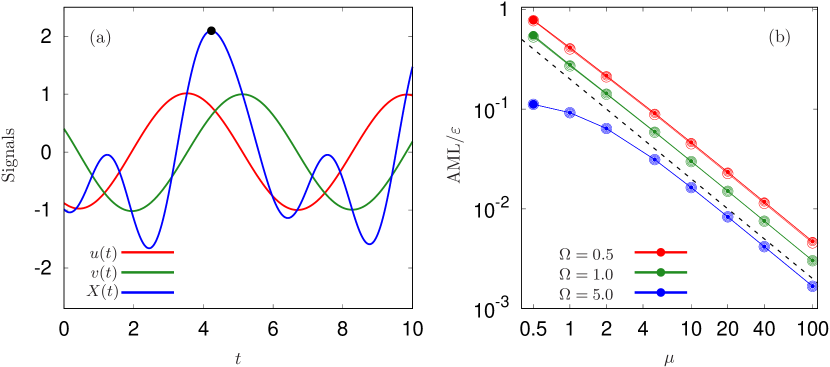
Figure 1: Panel (a): The time series of variables $u(t),v(t)$ and of observable $X(t)$ (Eq. 10) for the SLO with $\alpha=0.1$, $\mu=0.5$, $\Omega=0.5$ and $\varepsilon=0.1$. The bold black dot indicates a marker event that corresponds to a phase of $k2\pi$, this marker event will be used below for the protophase definition. Because only a short piece of about one period is depicted, the modulation is not visible at this scale. Panel (b): Levels of the amplitude modulation, AML (cf. Eq. (13)), in the driven SLO Eqs. (6), (11) with observable from Eq. (10). The curves show AML normalized by the amplitude of the forcing $\varepsilon$, for four values of $\varepsilon=0.01,\;0.02,\;0.05,\;0.1$ (different dot sizes, they overlap nearly perfectly) and for three values of the forcing frequency as indicated in the panel. The dashed line shows the power law $0.2\mu^{-1}$.

In case of the SLO, the curves for different $\varepsilon$ nearly perfectly overlap, showing that the AML is $\propto\varepsilon$. This level decreases with parameter $\mu$ as $\propto\mu^{-1}$. Thus, in the limit $\mu\to\infty$, the observable is purely phase modulated.

4 Protophases and the Phase Reconstruction Problem

According to the theory summarized in Section 2, the phase is defined as a $2\pi$-periodic variable which grows uniformly if the dynamics is unperturbed, i.e. if amplitude perturbations vanish. For example, for the SLO (6), if variables $(u(t),v(t))$ on the limit cycle are observed, the definition $\phi=\text{arg}(u+iv)$ provides the true phase. If, however, the observed variables are slightly shifted, then the same definition $\phi^{\prime}=\text{arg}(u+u_{0}+i(v+v_{0}))$ will provide a phase variable which is not growing uniformly in time, although it is $2\pi$-periodic. This observation motivated authors of Refs. [32, 33] to introduce a notion of protophase as a variable that parametrizes motion on a limit cycle, which is $2\pi$-periodic and monotonously – but not uniformly – grows in time. Generally, a protophase depends on the details of its definition (in the example above on the values of the offset $(u_{0},v_{0})$, but as a rule also on the observables used, on the way one defines a coordinate along a closed curve, etc.). Thus, it is convenient to introduce a family of protophases [32, 33], which can be obtained from the phase via a transformation

$$\psi=\Psi(\varphi),\qquad\text{where}\quad\Psi(\varphi)=\Psi(\varphi+2\pi)+2\pi\;,\;\;\Psi^{\prime}>0\;.$$ (14)

For any admissible function $\Psi$, the variable $\psi$ will be an admissible protophase, fulfilling the condition of $2\pi$-periodicity. Generally, one can assume that a reconstruction method delivers some protophase $\psi$, not the true phase $\varphi$ [32, 33].

In fact, a reconstruction of a protophase already provides a very rich knowledge on the dynamics, because the genuine phase is related to it via a one-to-one transformation of class (14). For example, one could reconstruct dynamical equations of type (4) in terms of a protophase. The disadvantage is that these dynamical equations are not observable-independent (because protophase-dependent), and cannot be compared directly with theory, in contradistinction to the equations for the true phase.

Therefore, the phase dynamics reconstruction problem can be divided into two steps:

1. From a generic observation $X(t)$ of a dynamical system with a limit cycle, infer a protophase $\psi(t)$ that is a function of the genuine phase $\varphi$.

2. Having obtained a protophase $\psi$, find a transformation to the genuine phase $\psi\to\varphi$.

We will address problem 1 in Sections 5 and 6 below. First, in Section 5 we will consider the case of a purely phase-modulated observable and present the method of Iterated Hilbert Transform Embeddings (IHTE), which solves the problem [31]. Then in Section 6 we will explore, how well this method works for observables with an additional amplitude modulation. Finally, in Section 7, we will discuss the protophase-to-phase transformation problem [32, 33].

5 Phase Demodulation via Iterated Hilbert Transform Embeddings

Here we consider the problem of phase reconstruction for a purely phase-modulated signal. Because, as discussed above, generally we have no chance to obtain the true phase, we from the beginning write this signal as a function of a protophase

$$X(t)=S(\psi(t)),\quad S(\psi)=S(\psi+2\pi)\;.$$ (15)

This signal corresponds to observations of the state of an oscillator, if on the r.h.s. of expressions (5) and (12) only the first term is present. The $2\pi$-periodic function $S$ will be called waveform. Of course, if another protophase is used, the waveform changes as well. The goal is to find one protophase and one waveform from this family.

5.1 Case of two observables

The solution of this problem is simple, if a second observable $Y(t)=S_{y}(\psi(t))$, also only purely phase-modulated, would be available (this second observable should be of course at least partially independent of the first one). Then, the trajectory $(X(t),Y(t))$ on the plane $(X,Y)$ will be, according to the Whitney’ embedding theorem [34], a closed curve (although possibly with self-crossings) and the protophase $\psi(t)$ can be chosen as some parametrization along this curve. For example, the curve length

$$L(t)=\int_{0}^{t}\sqrt{\dot{X}^{2}+\dot{Y}^{2}}dt$$ (16)

yields a monotonously growing function of time, even if the curve has many loops (i.e., if the waveform is complex). The protophase can then be defined as

$$\psi(t)=2\pi\frac{L(t)}{\mathcal{L}}\;,$$ (17)

where $\mathcal{L}$ is the total length of the closed loop and thus can be obtained from data. As has been discussed previously in [31], it stands in close correspondence to the average periodicity of the signal in terms of $L$. We stress here that for determining the protophase (17) no a priori knowledge on the properties of the system is needed.

5.2 Hilbert transform embedding

If only one scalar time series $X(t)$ is available, one tries to´ obtain the second scalar time series $Y(t)$ from the first one. The most widely used method for this task is the Hilbert transform (HT): $Y(t)=\hat{H}[X(t)]$, where

$$\hat{H}[X(t)]=\frac{\text{p.v.}}{\pi}\int_{t^{(0)}}^{t^{(m)}}\frac{X(\tau)}{t-\tau}d\tau\;.$$ (18)

(Formally, the HT is defined on an infinite time interval, we write here finite limits $t^{(0)}$, $t^{(m)}$ because we will apply it to a finite time series).

After calculating $Y(t)$, one performs an embedding on the plane $(X,Y)$. The main problem with this approach is that – already for a purely phase-modulated signal – the HT embedding is not a closed curve, but rather a band (see Fig. 2 a,b). The reason for this is the well-known fact that the HT mixes modulations of amplitude and phase [28, 29, 30, 15]. Thus, any definition of a protophase based on the embedding $(X,\hat{H}[X])$ is not accurate.

5.3 Iterated Hilbert transform embeddings

To resolve the problem, in Ref. [31] we demonstrated, theoretically and numerically, how an iteration of the HT embedding yields an almost perfect phase demodulation for purely phase modulated signals. In this procedure, remaining errors arise due to a discrete implementation of the HT and the finiteness of the time series. The main idea is to use the approximate phase, obtained from the embedding $(X,Y)$, as a new “time” variable, and perform a new HT in terms of this new time.

To describe the procedure algorithmically, it is convenient to introduce a protophase at each step of iterations $\theta_{n}$, and to treat time as the zero-order protophase $\theta_{0}=t$. Then, at each step $n$ one has a signal $X(\theta_{n})$. The HT of this signal is calculated according to

$$Y(\theta_{n})=\hat{H}[X(\theta_{n})]=\frac{\text{p.v.}}{\pi}\int_{\theta_{n}^{(0)}}^{\theta_{n}^{(m)}}\frac{X(\tilde{\theta}_{n})}{\theta_{n}-\tilde{\theta}_{n}}\ d\tilde{\theta}_{n}\;.$$ (19)

Here one should take into account that for different $n$ the functions $X(\theta_{n})$ are different. For simplicity of notations, we keep this difference only by writing the corresponding index at the argument, the same holds for $Y(\theta_{n})$. After $Y(\theta_{n})$ is calculated, we perform an embedding in the plane $(X(\theta_{n}),Y(\theta_{n}))$ and calculate the (non-normalized) protophase at the next step as the length along the embedded trajectory, like in (16):

$$L_{n+1}(\theta_{n})=\int_{0}^{\theta_{n}}\sqrt{(dX/d\theta_{n}^{\prime})^{2}+(dY/d\theta_{n}^{\prime})^{2}}d\theta_{n}^{\prime}\;.$$ (20)

In principle, for further iterations it is not necessary to normalize $L_{n+1}(\theta_{n})$, because the outcome of the integration Eq. (19) is independent on the rescaling of the argument. It is, however, convenient for the sake of comparison and of presentation, to have at each step a protophase normalized to intervals of $2\pi$. We employ an approach based on a spline interpolation. We define for each period one marker event (in the context of stochastic processes, a slightly different, statistical concept of marker events is used [35, 36]). Practically, we take as this event the largest local maximum of the waveform on a period (as depicted in Fig. 1 (a)). Subsequent markers correspond to phases $0,2\pi,4\pi,\ldots,k2\pi,\ldots$. If these events correspond to the values of the quantities calculated in Eq. (20) $L_{n+1}^{(0)},L_{n+1}^{(1)},L_{n+1}^{(2)},\ldots,L_{n+1}^{(k)},\ldots$, then we define $\theta_{n+1}$ as a smooth function of $L_{n+1}$, having values $k2\pi$ at values of the argument $L_{n+1}^{(k)}$. We denote this spline normalization of the length-defined protophase as

$$\theta_{n+1}(t)=\text{SPL}(L_{n+1}(t))\;.$$ (21)

We accomplish the construction with standard cubic splines [37]. One can easily see, that if the embedding in the plane $(X(\theta_{n}),Y(\theta_{n}))$ is a well defined curve, then this definition of the protophase $\theta_{n+1}(t)$ coincides with Eq. (17) (because in this case the function (21) is a straight line). Notice, that in this procedure one calculates the values of the protophase $\theta_{n}(t)$ at the same instants, at which the initial time series was defined. In this way, applying steps Eqs. (19) - (21) iteratively for $n=0,1,2\ldots$, one obtains a series of the protophases $\theta_{n+1}(t)$ as functions of time. As has been demonstrated in Ref. [31], this procedure converges to an almost perfectly $2\pi$-periodic protophase.

Before applying this method to observations, of the driven SLO, we illustrate it with a purely phase-modulated signal like in Eq. (15).

5.4 Example - A purely phase-modulated signal

Here we demonstrate properties of the IHTE using a purely phase modulated signal. We create it from the dynamics of the forced SLO (Section 3). We use the basic observable (10), but insert there purely phase-dependent variables

$$\overline{u}(t)=\cos(\varphi(t)),\quad\overline{v}=\sin(\varphi(t)),\quad\overline{X}=\overline{u}^{3}+\overline{v}+2\overline{u}\overline{v}\;.$$

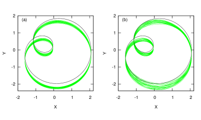
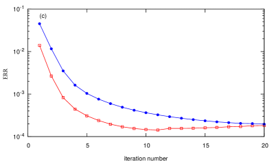
Figure 2: Panels (a) and (b): illustration of embeddings in plane $(\overline{X}(\theta_{n}(t)),\overline{Y}(\theta_{n}(t))$ for the first iteration $(n=1)$ (green line) and for the final iteration $n=20$ (black line). Panel (a): $\Omega=1$; panel (b): $\Omega=4$. One can see that at the first iteration a certain level of amplitude modulation appears (one observes a band of a finite width). At $n=20$ the line is nearly perfect, indicating for a very low level of residual amplitude modulation. Panel (c): Characterization of quality of the phase demodulation by periodicity error ERR (22). Filled circles: $\Omega=4$, open squares: $\Omega=1$.

We characterize the success of the phase demodulation procedure in two ways, at each step of the iterative procedure where the approximate protophase $\theta_{n}(t)$ is determined. The first method is just a visualization of the embedding $(\overline{X}(\theta_{n}(t)),\overline{Y}(\theta_{n}(t)))$. For a perfect demodulation, this embedding produces a closed loop describing the waveform of the signal (cf. discussion in Section 5.1). In a more quantitative approach, the success of demodulation is determined by the periodicity error

$$(\text{ERR}_{n})^{2}=\frac{\int[X(\theta_{n}+2\pi)-X(\theta_{n})]^{2}d\theta_{n}}{\int[X(\theta_{n})-\langle X\rangle]^{2}d\theta_{n}}\;.$$ (22)

This expression is similar to the AML Eq. (13). We stress here, that this expression is based on the observations only and does not require a priori knowledge of the system. The difference is that it now monitors the $2\pi$-periodicity of the waveform $X(\theta_{n})$ which is an indicator for the remaining spurious amplitude modulation of the reconstructed waveform in step $n$. If $2\pi$-periodicity is achieved, then ERR_n is zero.

We illustrate the results for the driven SLO (6),(11) with $\varepsilon=0.3$ and two values of the basic frequency of the forcing $\Omega\in\left\{1,4\right\}$ in Fig. 2. Compared to the basic period of oscillations, these forcing frequencies give rise to a slow (case $\Omega=1$) and a fast (case $\Omega=4$) forcing, respectively. The obtained results confirm findings of Ref. [31], which can be summarized as follows: (i) For a slow (i.e. $\Omega\lesssim 1$) and weak (i.e. $\varepsilon\ll\omega$) modulation, already the first iteration (i.e. the traditional HT embedding) provides the highest periodicity of the protophase (e.g., in Fig. 2(c) ERR₁ in the first iteration for $\Omega=1$ is approximately 4 times smaller than for $\Omega=4$, with the same amplitude of the forcing); (ii) for all other cases, i.e. for a slow (i.e. $\Omega\lesssim 1$) but strong (i.e., $\varepsilon\lesssim\omega$) modulation, as well as for a fast modulation (i.e. $\Omega>1$), several iterations are needed to achieve a good demodulation. The final level of the error is limited by errors in numerical performance of the HT due to discreteness and finiteness of the signal.

6 Protophase reconstruction from the full signal

Here we report on the application of the IHTE procedure to the time series of the observable $X(t)$ (10) from the forced SLO. As the observable contains both a phase and an amplitude modulation, we cannot expect that the resulting modulation error (22) will be small; in fact it is bounded below by the amplitude modulation level. The question we would like to address is whether iterations improve the quality of the protophase reconstruction. We show the results in Figures 3, 4. Figure 3 shows the error according to (22) versus the iteration number for different values of the driving frequency $\Omega$ and of the parameter of stability of the limit cycle $\mu$. One can see that for a slow forcing (panel (b), $\Omega=1$), a weak improvement is achieved for large $\mu=64$ only, i.e., for a weak amplitude modulation. In all other cases, already the first iteration provides a reconstruction that cannot be further improved. On the other hand, for higher frequency of the forcing (panel (a)), and for large enough values of stability parameter $\mu\in\left\{16,64\right\}$, iterations do indeed improve the quality of the reconstruction - by one order of magnitude for $\mu=64$. This general conclusion is supported also by Fig. 4, which shows, in dependence on $\mu$, the periodicity error ERR_n after the 1st and the last ($n=20$) iteration steps. From this data one can see how significant the improvement is due to IHTE for extremely large stability of the limit cycle ($\mu=128$). An improvement is already present for $\mu>4$ for $\Omega=4$, and for $\mu>16$ for $\Omega=1$.

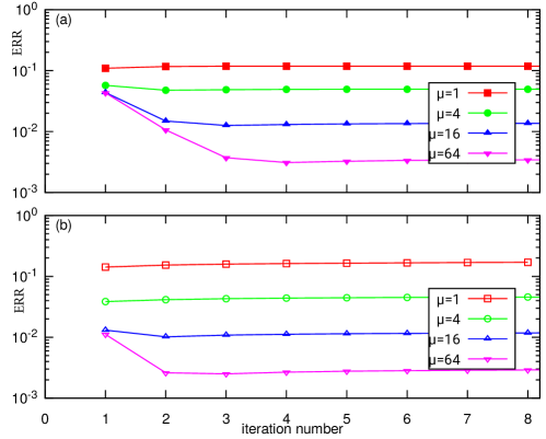
Figure 3: Periodicity error ERR_n for the phase reconstruction by virtue of the IHTEs. Panel (a): $\Omega=4$, panel (b) $\Omega=1$.

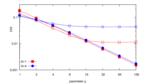
Figure 4: Periodicity error ERR_n in the protophase reconstruction in dependence on parameter $\mu$: ERR₁ at iteration step $n=1$ is shown with open markers, and error Err₂₀ at iteration step $n=20$ is shown with corresponding filled markers.

7 Protophase-to-Phase Transformation

After having obtained a protophase $\psi(t)=\theta_{n}(t)$ from IHTE as described in Section 5.3 above, the true phase needs to be estimated. We assume that any good protophase is a function of the true phase $\psi=\Psi(\varphi)$. Thus, the problem can be reformulated in terms of finding the inverse protophase-to-phase (PTP) transformation $\varphi=\Psi^{-1}(\psi)$.

7.1 Two variants of PTP transformation

In Ref. [32, 33], a method to reconstruct the protophase-to-phase transformation (PTP) $\Psi^{-1}(\psi)$ has been suggested. It is based on the assumption that the phase probability distribution density $\rho(\varphi)$ should be uniform: $\rho(\varphi)=(2\pi)^{-1}$. This condition indeed selects the true phase for an undriven oscillator: because $\dot{\varphi}=\omega$, the density of $\varphi$ is uniform. Next, one assumes that under small forcing the distribution is only slightly perturbed such that uniformity should be valid at least up to corrections $\sim\varepsilon$ [32, 33].

Practically, implementation of the PTP according to the condition of uniformity is based on the estimation of the density of the protophase $\rho(\psi)$ [32, 33]. It is convenient to represent this density via $K$ Fourier modes, the amplitudes $F_{k}$, $k=1,\ldots,K$ of which are calculated directly from the time series of the protophase $\psi(t)$:

$$F_{k}=\frac{1}{2\pi}\int_{0}^{2\pi}\rho(\tilde{\psi})\exp(-ik\tilde{\psi})d\tilde{\psi}=\frac{1}{t^{(m)}-t^{(0)}}\int_{t^{(0)}}^{t^{(m)}}\exp(-ik\psi(t))dt\;.$$ (23)

After this, the PTP transformation is accomplished according to the expression [32, 33]

$$\varphi=\Psi^{-1}(\psi)+\xi^{db}(\psi)=\int_{0}^{\psi(t)}\rho(\tilde{\psi})d\tilde{\psi}+\xi^{db}(\psi)=\psi+\sum^{K}_{k\neq 0}\frac{F_{k}}{ik}\Big{(}\exp(ik\psi)-1\Big{)}+\xi^{db}(\psi)\;.$$ (24)

The residual term of this density-based PTP is denoted by $\xi^{db}(\psi)$.

The PTP transformation (23),(24) has the advantage that it is purely data-based; thus, on the one hand, no additional information is needed. On the other hand, it is based on a condition (uniform density of the true phase), that is fulfilled only approximately. To evaluate the quality of the data-driven PTP, we additionally estimate the coefficients of the mapping $\Psi^{-1}(\psi)$ from the least square fit to $\varphi$, according to the following expression:

$$\Big{\langle}\left[\varphi(t)-\psi(t)-\sum^{K}_{k=0}A_{k}\cos(k\psi(t))+B_{k}\sin(k\psi(t))\right]^{2}\Big{\rangle}_{t}\rightarrow\text{min}\;.$$ (25)

(We used the C++ library EIGEN to perform this task.) The residual term of fitting here is denoted as $\xi^{fit}(\psi)$. We would like to stress that this approach makes use of $\varphi(t)$ and is thus based on theoretical information, not available in an experiment. However, it can be deemed as the optimal PTP because it is not bound to the condition of uniformity for $\rho(\psi)$ discussed before.

7.2 Accuracy of phase reconstruction

Here in Fig. 5 we present exemplary residua $\xi^{fit,db}(\psi(\varphi))$ of phase reconstructions after PTP from the direct fitting Eq. (25) and from the density-based approach Eq. (24) (both with $K=30$) for signals $X(t)$ at different frequencies of the forcing, $\Omega$, and of the oscillator stability $\mu$. In accordance with the results of Section 6 above, only for forcing frequencies larger than the base frequency, and for large values of parameter $\mu$, i.e. for strong stability of the limit cycle, the iterations of the IHTE allow for an essential improvement. Moreover, for the case of low-frequency forcing, the two variants of the PTP transformation give very similar results. We attribute this to the fact that the uncertainty in the protophase reconstruction is significantly larger than the violation of the uniformity condition for the density of the true phase.

For the high-frequency forcing, the results of the two variants of the PTP transformation are slightly different. It is instructive to compare panels (h) (direct fit according to (25)) and (i) (density-based transformation according to (24)). For the direct fit, the residual error does not depend on average on $\varphi$, thus it is intrinsic and cannot be removed by an additional transformation. In contradistinction, the curve of the density-based fit shows pronounced oscillations and could be potentially improved. This residual waveform is due to non-exactness of the condition of uniform density of the true phase.

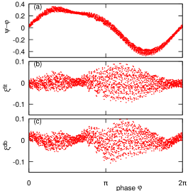
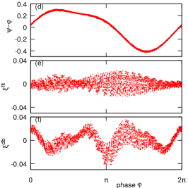
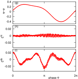
Figure 5: Panels (a,d,g): Differences $\psi-\varphi$ obtained in the IHTE procedure vs the true phase $\varphi$. Here, $\psi=\theta_{20}$ after 20 iterations. Panels (b,e,h): Residua $\xi^{fit}(\psi(\varphi))$ obtained by applying to the protophase $\psi$ the fitting procedure (25). Panels (c,f,i): Residua $\xi^{db}(\psi(\varphi))$ obtained by applying to the protophase $\psi$ the PTP procedure (24). Parameter of the forcing is $\Omega=4$, parameters of the SLO: in panels (a,b,c) $\mu=4$, in panels (d,e,f) $\mu=16$, and in panels (g,h,i) $\mu=64$. Notice that the panels showing the residua have different vertical scales for different values of $\mu$. In all panels, many periods of the signal are overlapped.

Finally, to judge the accuracy of the combined procedure of IHTE and PTP transformation, we define the phase reconstruction error PRE as the variance of the difference $\Psi^{-1}(\theta_{n})-\varphi$:

$$\text{PRE}_{n}^{2}=\langle(\Psi^{-1}(\theta_{n})-\varphi-\langle\Psi^{-1}(\theta_{n})-\varphi\rangle)^{2}\rangle,$$ (26)

and plot it vs the iteration number in Fig. 6. For a small forcing frequency ($\Omega=1$), practically no improvement via iterations is achieved. One can see here that the overall accuracy grows significantly with parameter $\mu$, i.e. with the increasing stability of the limit cycle. Panel (a) shows that for a higher forcing frequency ($\Omega=4$), the reconstruction error reduces by a factor of two to three within the first five iterations.

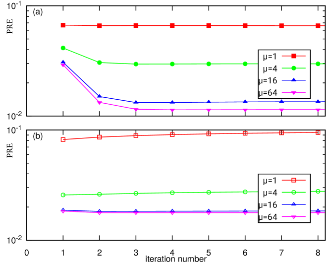
Figure 6: Reconstruction error (26) for phase estimation by virtue of the IHTEs and subsequent PTP transformation according to (26). Panel (a): $\Omega=4$, panel (b) $\Omega=1$. The values of the SLO parameter $\mu$ are depicted in the panels.

As a visual example for the accuracy of reconstruction, Fig. 7 depicts the true phase together with reconstructions at the 1st and at the 20th iterations.

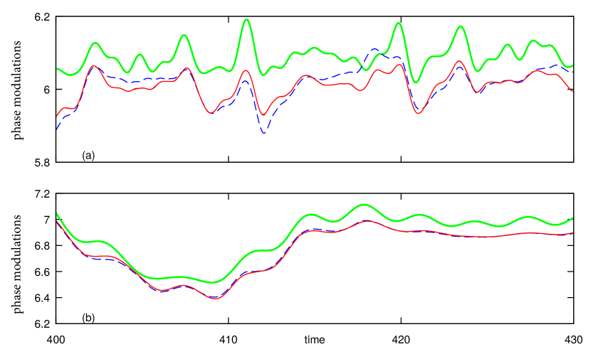
Figure 7: Comparison of the true phase (green line) with phases obtained after the protophase reconstruction at the 1st iteration of the IHTE procedure (blue dashed line) and at iteration 20 (red line). To the protophases also the density-based PTP transformation according to expressions (23) has been applied. We removed the linear trend $\sim t$ from all phases and we shifted the true phase vertically for better comparison. Panel (a): $\Omega=4$, panel (b): $\Omega=1$.

8 Conclusion

The goal of this study was to explore how phase reconstruction from scalar observables of oscillatory dynamical systems can be improved by the application of iterated Hilbert transform embeddings. We considered the simplest model of stable self-oscillations, the Stuart-Landau oscillator, under quasiperiodic external forcing. We explored a range of the frequencies of the forcing and of the limit cycle stability parameter. The main conclusion is the following: In the case of purely phase-modulated signals, the true phase can be nearly perfectly reconstructed. In the more realistic situation where modulations of the amplitude and of the phase are present, the improvement from IHTEs is moderate if any.

Because the amplitude modulation is heavily suppressed in the case of highly stable limit cycles, we have observed that for large values of $\mu$ IHTEs indeed enhance the quality of phase reconstruction. However, for small $\mu$ there is no merit in performing iterations. The reason for this is that the Hilbert transform (HT) “mixes” phase and amplitude modulations, and iterations beneficial in the purely phase-modulated case are spoiled by the intrinsic amplitude modulation of the signal. Practically, we could recommend performing at least one additional iteration of the HT embedding, and if it does not reduce the error, use just the phase from the first HT. Otherwise, one can perform several iterations until ERR_n stops to decrease. Albeit there exists no strict correspondence between the periodicity error ERR_n Eq. (22) and the reconstruction accuracy PRE_n Eq. (26), we suggest that the empiric criterion for ERR_n, put forward in this study, should be used to test protophases for their quality ($2\pi$-periodicity).

Here, we would like to stress several aspects of our approach which are either not widespread in the literature or should be taken into account when developing further the IHTE procedure:

1. We used a scalar observable of moderate complexity, which is a smooth function of the system variables. The observed signal thus does not have a simple sine-like form but has several maxima and minima on the basic period. Correspondingly, an embedding using HT leads to a “band” that has several loops. In such a situation one cannot use the argument of the analytic signal $X+i\hat{H}[X]$ for the phase estimation. Instead, we used the length of the curve as an estimation of the protophase, following Refs. [12, 31].

2. It is important to distinguish a protophase, $\psi(t)$, which is the final result of successful phase demodulation (Section 5), and an estimate of the true phase $\varphi(t)$. The true phase is just one out of a family of possible protophases, and typically does not arise through the demodulation procedure described above. While all the protophases are equivalent (up to an invertible transformation), knowing the true phase is of enormous merit, because this allows one to obtain from the data a description as close as possible to the theory. In this work, we used a density-based transformation from a length-defined protophase to the phase [33] and demonstrated that it gives rise to small deviations from the ground truth. The remaining deviations arise due to the basic assumption behind this approach, namely that the true phase has a uniform distribution, which is valid only approximately. Due to this, we used different measures of accuracy to characterize the quality ($2\pi$-periodicity) of the protophase reconstruction (ERR_n), and the quality of the protophase-to-phase transformation (PRE_n) throughout iterations.

3. We would like to point out that three levels of error estimation have been outlined in this paper. First, one can compare the width of the embedding curve in the first and the final step of iterations. This approach might be useful if just a rough idea is needed on how good demodulation is. Second, a quantitative and data-driven measure for the periodicity of a protophase is defined by the quantity ERR (Eq. (22)). This measure does not assume any a priori knowledge of the system’s properties. In contradistinction, the absolute reconstruction error PRE (Eq. (26)) is measured directly for the true phase $\varphi$. It is thus not applicable in studies of empirical data but can be calculated and compared to ERR if the dynamical equations are known.

4. We would like to stress that iterated embeddings in the IHTE are different from the embeddings used for a phase space representation of a high-dimensional attractor [38]. Because we study (modulated) periodic oscillations, in the ideal case of pure phase modulation, the underlying object is a one-dimensional manifold, which, according to Whitney’s embedding theorem [34], can be embedded in a two-dimensional plane. A Hilbert transform allows for a two-dimensional representation, but due to a mixture of phase and amplitude modulations, it does not provide a good embedding at the first step. This drawback is cured by adopting the iteration procedure according to Ref. [31].

As discussed above, resolving the amplitude modulation problem remains the main challenge in constructing an accurate phase reconstruction from data. However, it appears promising to attack this problem for situations where there is sufficient theoretical understanding of the amplitude dynamics in coupled oscillators. In particular, the theory of higher-order interactions of coupled Stuart-Landau oscillators [25] includes explicit expressions for the amplitude variations in low orders in the coupling parameter; this information could be used to develop and validate methods of coping with the amplitude modulation.

Moreover, we have shown that, despite a significant increase in the protophase periodicity due to IHTE, the pre-assumptions of data-driven PTP represent a potential obstacle for an accurate phase reconstruction. These results suggest improving the PTP procedure to non-uniform target phase densities and/or incorporating phase-amplitude coupling into the phase reconstruction. To the best of our knowledge, both approaches are unsolved problems. Particularly, the highly desirable data-driven reconstruction of a phase-amplitude coupling from geometric information of embedding curves is an open problem. Some work has been carried out given full observations of the limit cycle dynamics [39].

In this paper, we assumed that the available time series is an observable of a perturbed oscillating dynamical system. Therefore we did not touch the issue of preprocessing the data if this assumption is not fulfilled. In the case where the time series is a mixture of components from different oscillators, one could try to separate these components using signal decomposition methods (like empirical mode decomposition [14], intrinsic mode functions [40], Hilbert-Huang transform [41]). However, it is not clear how such a preprocessing affects the properties of the phase and the amplitude modulations that are crucial for phase extraction. Quite popular are also methods of time-frequency analysis, based on the wavelet transform; they aim at finding an instantaneous frequency of a signal [42, 43]. These methods typically provide a frequency averaged over several characteristic periods. Potentially, one could reconstruct a protophase by integration of the instantaneous frequency. Comparing the wavelet-based methods and the Hilbert transform-based technique described above remains a subject for future studies.

Finally, we would like to stress that the phase dynamics concepts have been extended for chaotic oscillators and systems with strong noise [44, 45]. However, in these cases, the amplitude modulation of the observed signals is very strong, and we do not expect the IHTEs to improve the phase reconstruction task.

Bibliography

Bibliography

- [1] M. H. Matheny, J. Emenheiser, W. Fon, A. Chapman, A. Salova, M. Rohden, J. Li, M. H. de Badyn, M. P’osfai, L. Duenas-Osorio, M. Mesbahi, J. P. Crutchfield, M. C. Cross, R. M. D’Souza, M. L. Roukes, Exotic states in a simple network of nanoelectromechanical oscillators, Science 363 (2019) eaav7932.
- [2] N. Blackbeard, S. Wieczorek, H. Erzgräber, P. S. Dutta, From synchronisation to persistent optical turbulence in laser arrays, Physica D: Nonlinear Phenomena 286 (2014) 43–58.
- [3] M. Nixon, E. Ronen, A. A. Friesem, N. Davidson, Observing geometric frustration with thousands of coupled lasers, Phys. Rev. Lett. 110 (2013) 184102.
- [4] J. L. Ocampo-Espindola, C. Bick, I. Z. Kiss, Weak chimeras with modular electrochemical oscillator networks, Frontiers in Applied Mathematics and Statistics 5 (2019) 38.
- [5] O. E. Omel’chenko, M. Sebek, I. Z. Kiss, Universal relations of local order parameters for partially synchronized oscillators, Phys. Rev. E 97 (6).
- [6] K. A. Blaha, A. Pikovsky, M. Rosenblum, M. T. Clark, C. G. Rusin, J. L. Hudson, Reconstruction of two-dimensional phase dynamics from experiments on coupled oscillators, Phys. Rev. E 84 (4) (2011) 046201.
- [7] S. H. Strogatz, D. M. Abrams, A. McRobie, B. Eckhardt, E. Ott, Crowd synchrony on the millennium bridge, Nature 438 (7064) (2005) 43–44.
- [8] E. Lowet, M. J. Roberts, P. Bonizzi, J. Karel, P. De Weerd, Quantifying Neural Oscillatory Synchronization: A Comparison between Spectral Coherence and Phase-Locking Value Approaches, PLOS ONE 11 (1).
- [9] R. van der Meij, J. Jacobs, E. Maris, Uncovering phase-coupled oscillatory networks in electrophysiological data, Human Brain Mapping 36 (7) (2015) 2655–2680.
- [10] D. Benitez, P. Gaydecki, A. Zaidi, A. Fitzpatrick, The use of the Hilbert transform in ECG signal analysis, Computers in Biology and Medicine 31 (5) (2001) 399–406.
- [11] Ç. Topçu, M. Frühwirth, M. Moser, M. Rosenblum, A. Pikovsky, Disentangling respiratory sinus arrhythmia in heart rate variability records, Physiological Measurement 39 (5) (2018) 054002.
- [12] B. Kralemann, M. Frühwirth, A. Pikovsky, M. Rosenblum, T. Kenner, J. Schaefer, M. Moser, In vivo cardiac phase response curve elucidates human respiratory heart rate variability, Nature Communications 4 (2013) 2418.
- [13] A. Yeldesbay, G. R. Fink, S. Daun, Reconstruction of effective connectivity in the case of asymmetric phase distributions, Journal of Neuroscience Methods 317 (2019) 94–107.
- [14] B. M. Battista, C. Knapp, T. McGee, V. Goebel, Application of the empirical mode decomposition and Hilbert-Huang transform to seismic reflection data, Geophysics 72 (2) (2007) H29–H37.
- [15] D. A. Zappala, M. Barreiro, C. Masoller, Mapping atmospheric waves and unveiling phase coherent structures in a global surface air temperature reanalysis dataset, Chaos: An Interdisciplinary Journal of Nonlinear Science 30 (1) (2020) 011103.
- [16] S. Shahal, A. Wurzberg, I. Sibony, H. Duadi, E. Shniderman, D. Weymouth, N. Davidson, M. Fridman, Synchronization of complex human networks, Nature communications 11 (1) (2020) 1–10.
- [17] H. Kantz, T. Schreiber, Nonlinear Time Series Analysis, Cambridge University Press, Cambridge, 2004, 2nd edition.
- [18] M. Rosenblum, A. Pikovsky, Detecting direction of coupling in interacting oscillators, Phys. Rev. E 64 (4) (2001) 045202(R).
- [19] W. D. Penny, V. Litvak, L. Fuentemilla, E. Duzel, K. Friston, Dynamic causal models for phase coupling, J. Neurosci. Methods 183 (2009) 19–30.
- [20] T. Stankovski, T. Pereira, P. V. E. McClintock, A. Stefanovska, Coupling functions: Universal insights into dynamical interaction mechanisms, Rev. Mod. Phys. 89 (2017) 045001.
- [21] Y. Kuramoto, Chemical Oscillations, Waves and Turbulence, Springer, Berlin, 1984.
- [22] A. Pikovsky, M. Rosenblum, J. Kurths, Synchronization: a universal concept in nonlinear sciences, Cambridge University Press, 2001.
- [23] H. Nakao, Phase reduction approach to synchronisation of nonlinear oscillators, Contemporary Physics 57 (2) (2016) 188–214.
- [24] B. Pietras, A. Daffertshofer, Network dynamics of coupled oscillators and phase reduction techniques, Physics Reports 819 (2019) 1–105.
- [25] E. Gengel, E. Teichmann, M. Rosenblum, A. Pikovsky, High-order phase reduction for coupled oscillators, Journal of Physics: Complexity 2 (1) (2020) 015005.
- [26] M. Feldman, Hilbert transform applications in mechanical vibration, John Wiley & Sons, 2011.
- [27] F. W. King, Hilbert Transforms, Vol. 1,2 of Encyclopedia of Mathematics and its Applications, Cambridge University Press, 2009.
- [28] E. Bedrosian, The analytic signal representation of modulated waveforms, Proceedings of the IRE 50 (10) (1962) 2071–2076.
- [29] E. Bedrosian, A product theorem for Hilbert transforms, Proceedings of the IEEE 51 (5) (1963) 868–869.
- [30] R. Guevara Erra, J. L. Perez Velazquez, M. Rosenblum, Neural synchronization from the perspective of non-linear dynamics, Frontiers in computational neuroscience 11 (2017) 98.
- [31] E. Gengel, A. Pikovsky, Phase demodulation with iterative Hilbert transform embeddings, Signal Processing 165 (2019) 115–127.
- [32] B. Kralemann, L. Cimponeriu, M. Rosenblum, A. Pikovsky, R. Mrowka, Uncovering interaction of coupled oscillators from data, Phys. Rev. E 76 (5) (2007) 055201.
- [33] B. Kralemann, L. Cimponeriu, M. Rosenblum, A. Pikovsky, R. Mrowka, Phase dynamics of coupled oscillators reconstructed from data, Phys. Rev. E 77 (6) (2008) 066205.
- [34] M. Adachi, Embeddings and Immersions, AMS, 1993.
- [35] L. Callenbach, P. Hänggi, S. J. Linz, J. A. Freund, L. Schimansky-Geier, Oscillatory systems driven by noise: Frequency and phase synchronization, Physical Review E 65 (5) (2002) 051110.
- [36] S. O. Rice, Mathematical analysis of random noise, Bell Syst. Tech. J. 23 (3) (1944) 282–332.
- [37] W. H. Press, S. A. Teukolsky, W. T. Vetterling, B. P. Flannery, Numerical recipies in C, Vol. 3, Cambridge university press Cambridge, 1992.
- [38] T. Sauer, J. A. Yorke, M. Casdagli, Embedology, Journal of statistical Physics 65 (3) (1991) 579–616.
- [39] R. Cestnik, Inferring oscillatory dynamics from data, Ph.D. thesis, Vrije Universiteit Amsterdam (2020).
- [40] A. Stallone, A. Cicone, M. Materassi, New insights and best practices for the successful use of Empirical Mode Decomposition, Iterative Filtering and derived algorithms, Scientific Reports 10 (2020) 15161.
- [41] N. E. Huang, S. S. P. Shen (Eds.), Hilbert-Huang transform and its applications, World Scientific, Singapore, 2014.
- [42] M. Le Van Quyen, J. Foucher, J.-P. Lachaux, E. Rodriguez, A. Lutz, J. Martinerie, F. J. Varela, Comparison of Hilbert transform and wavelet methods for the analysis of neuronal synchrony, Journal of Neuroscience Methods 111 (2) (2001) 83–98.
- [43] I. Daubechies, J. Lu, H.-T. Wu, Synchrosqueezed wavelet transforms: An empirical mode decomposition-like tool, Appl. Comput. Harmon. Anal. 30 (2011) 243–261.
- [44] J. T. Schwabedal, A. Pikovsky, B. Kralemann, M. Rosenblum, Optimal phase description of chaotic oscillators, Phys. Rev. E 85 (2) (2012) 026216.
- [45] J. T. Schwabedal, A. Pikovsky, Phase description of stochastic oscillations, Phys. Rev. Lett. 110 (20) (2013) 204102.