Data-driven analysis of a SUSY GUT of flavour

Abstract

We present a data-driven analysis of a concrete Supersymmetric (SUSY) Grand Unified Theory (GUT) of flavour, based on $SU(5)\times S_{4}$, which predicts charged fermion and neutrino mass and mixing, and where the mass matrices of both the Standard Model and the Supersymmetric particles are controlled by a common symmetry at the GUT scale. This framework also predicts non-vanishing non-minimal flavour violating effects, motivating a sophisticated data-driven parameter analysis to uncover the signatures and viability of the model. This computer-intensive Markov-Chain-Monte-Carlo (MCMC) based analysis includes a large range of flavour as well as dark matter and SUSY observables, predicts distributions for a range of physical quantities which may be used to test the model. The predictions include maximally mixed sfermions, $\mu\rightarrow e\gamma$ close to its experimental limit and successful bino-like dark matter with nearby winos (making direct detection unlikely), implying good prospects for discovering winos and gluinos at forthcoming collider runs. The results also demonstrate that the Georgi-Jarlskog mechanism does not provide a good description of the splitting of down type quark masses and charged leptons, while neutrinoless double beta decay is predicted at observable rates.

1 Introduction

The Minimal Supersymmetric Standard Model (MSSM) remains an appealing extension of the Standard Model of particle physics, as it provides solutions to the most prominent shortcomings of the latter. In addition to solving the hierarchy problem related to the mass of the Higgs boson HiggsATLAS2012 ; HiggsCMS2012 , the model includes a viable candidate for the observed Cold Dark Matter (CDM) in the Universe, namely the lightest of the four neutralinos. Furthermore, the masses of the Standard Model neutrinos can be generated through the Seesaw mechanism Minkowski:1977sc ; GellMann:1980vs ; Yanagida:1979as ; Mohapatra:1979ia ; Schechter:1980gr by including heavy right-handed neutrinos which can easily be implemented in the MSSM.

While collider searches for new physics have remained unsuccessful so far, additional information can be obtained from examining precision observables involving flavour transitions. For example, in the hadronic sector, the branching ratios of rare decays such as $b\to s\gamma$ are sensitive to new physics contributions, especially if they involve non-minimal flavour violation (NMFV), i.e. sources of flavour violation beyond the Cabbibo Kobayashi Maskawa (CKM) matrix Cabibbo1963 ; Kobayashi1973 . The same holds for the lepton sector Maki1962 ; Pontecorvo1967 , where NMFV contributions can induce the branching ratios like $\mu\to e\gamma$ and $\mu\to 3e$, or $\mu-e$ conversion rates in nuclei. Flavour precision observables therefore provide an interesting handle towards the new physics spectrum, and in particular towards the underlying flavour structure.

Extensive studies have shown that the MSSM parameter space can accomodate NMFV in both the squark and the slepton sectors despite the numerous experimental and theoretical constraints Arana-Catania:2014ooa ; Kowalska:2014opa ; DeCausmaecker:2015yca . In addition, NMFV may lead to specific collider signatures Bartl:2005yy ; Bozzi:2007me ; Bartl:2007ua ; delAguila:2008iz ; Hurth:2009ke ; Bartl:2009au ; Bruhnke:2010rh ; Bartl:2010du ; Bartl:2011wq ; Bartl:2012tx ; Bartl:2014bka , weaken the current mass limits derived from the non-observation of superpartners Blanke:2015ulx ; Brooijmans:2018xbu ; Chakraborty:2018rpn , and, although to some lesser extend, affect the dark matter phenomenology Barger:2009gc ; Choudhury2011 ; Herrmann:2011xe ; Agrawal:2014aoa .

A particularly interesting feature of the MSSM and related models is that they can be successfully embedded into Grand Unified Theories (GUTs). Such a framework allows a unification of the gauge couplings at a scale of about $10^{16}$ GeV with better precision than the Standard Model alone Amaldi:1991cn . In the same spirit, the soft breaking parameters related to squarks and sleptons stem from a common origin. In the most simple realizations this allows for the reduction of the number of parameters of the model. Starting from the imposed values at the GUT scale, the phenomenological aspects are obtained through renormalization group running to the TeV scale, where the physical masses and related observables are computed.

The two aforementioned aspects can be addressed by considering SUSY-GUTs including flavour symmetries, such as $SU(5)\times A_{4}$ Belyaev:2018vkl or $SU(5)\times S_{4}$ Dimou:2015cmw ; Dimou:2015yng , to cite only two examples. In such a situation, the flavour structure of the theory is defined at the GUT scale by the imposed symmetry. Renormalization group running then translates the GUT-scale structure into the observable mass spectrum at the TeV scale. The TeV-scale phenomenology thus inherits a footprint of the imposed flavour structure at the GUT scale.

In a previous study Bernigaud:2018qky , some of the authors have explored the phenomenology of NMFV within a $SU(5)\times A_{4}$ implementation of the MSSM suggested first in Ref. Belyaev:2018vkl . Based on the variation of the NMFV parameters around a MFV reference scenario taken from Ref. Belyaev:2018vkl , it has been shown that these parameters need to be varied simultaneously in order to cover all phenomenological aspects, in particular since cancellations between different contributions may occur. Moreover, it has been demonstrated that a model may feature a reasonable amount of flavour violation while satisfying the stringent constraints of rare decays such as $b\to s\gamma$ or $\mu\to e\gamma$ while sufficient lepton flavour violation may also address baryon asymmetry in the universe Mukaida:2021sgv . It is therefore interesting to pursue the study of GUT implementations of flavour violation, e.g., via flavour symmetries, in the context of low-energy and precision constraints as well as TeV-scale phenomenology.

In the present paper, we shall focus on the case of $SU(5)$ unification combined with an $S_{4}$ flavour symmetry, as suggested by one of the authors in Refs. Dimou:2015cmw ; Dimou:2015yng . In a similar way as in Ref. Bernigaud:2018qky , we will explore in detail the TeV-scale aspects of this model, including observables related to flavour violation and dark matter phenomenology. More precisely, in this study, we aim at a complete exploration of the associated parameters, i.e. including a variation of all relevant parameters at the GUT scale. For the sake of an efficient exploration, we make use of the Markov Chain Monte Carlo technique Metropolis1953 ; Hastings1970 ; Markov1971 .

The paper is organised as follows. In Section 2, we review the assumed model. Section 3 is dedicated to the discussion of the Markov Chain Monte Carlo algorithm that we employ to efficiently explore the model parameter space. Results are then presented in Section 4. Our conclusions are given in Section 5.

2 The Model

2.1 Fields and symmetries

The model developed in Refs. Hagedorn:2010th ; Hagedorn:2012ut ; Dimou:2015yng ; Dimou:2015cmw is based on the grand unifying group $SU(5)$ combined with an $S_{4}$ family symmetry, and supplemented by a $U(1)$ symmetry. The left-handed quarks and leptons are unified into the representations $\mathbf{\bar{5}}$, $\mathbf{10}$ and $\mathbf{1}$ of $SU(5)$ according to,

$$F_{\alpha}\sim\overline{\bf 5}\sim\left(\begin{array}[]{c}d_{r}^{c}\\ d_{b}^{c}\\ d_{g}^{c}\\ e^{-}\\ -\nu\end{array}\right)_{\!\!\alpha}\,,\qquad T_{\alpha}\sim{\bf 10}\sim\left(\begin{array}[]{ccccc}0&u_{g}^{c}&-u_{b}^{c}&u_{r}&d_{r}\\ .&0&u_{r}^{c}&u_{b}&d_{b}\\ .&.&0&u_{g}&d_{g}\\ .&.&.&0&e^{c}\\ .&.&.&.&0\end{array}\right)_{\!\!\alpha}\,,\qquad N_{\alpha}\sim{\bf 1}\sim\nu^{c}_{\alpha}$$ (2.11)

where the superscript $c$ stands for $CP$-conjugated fields (which would be right-handed without the $c$ operation), and $\alpha=1,2,3$ is a family index. The three families are controlled by a family symmetry $S_{4}$, with $F$ and $N$ each forming a triplet and the first two families of $T$ forming a doublet, while the third family $T_{3}$ (containing the top quark) is a singlet, as summarised in Table 1. The choice of the third family $T_{3}$ being a singlet, permits a renormalisable top quark Yukawa coupling to the singlet Higgs discussed below.

The $S_{4}$ singlet Higgs fields $H_{\bf{5}},\ H_{\bf{\bar{5}}}$ and $H_{\bf{\bar{45}}}$, each contain a doublet $SU(2)_{L}\times U(1)_{Y}$ representation that eventually form the standard up ($H_{u}$) and down ($H_{d}$) Higgses of the MSSM (where the $H_{d}$ emerges as a linear combination of doublets from the $H_{\bf{\bar{5}}}$ and $H_{\bf{\bar{45}}}$)  Chung:2003fi . The VEVs of the two neutral Higgs fields are

$$v_{u}=\frac{v}{\sqrt{1+t_{\beta}^{2}}}\,t_{\beta},~{}~{}~{}~{}~{}~{}v_{d}=\frac{v}{\sqrt{1+t_{\beta}^{2}}},$$ (2.12)

where $t_{\beta}\equiv\tan(\beta)=\frac{v_{u}}{v_{d}}$ and $v=\sqrt{v_{u}^{2}+v_{d}^{2}}\approx 246$ GeV.

Field

$T_{3}$

$T$

$F$

$N$

$H_{5}$

$H_{\overline{5}}$

$H_{\overline{45}}$

$\Phi_{2}^{u}$

$\widetilde{\Phi}_{2}^{u}$

$\Phi_{3}^{d}$

$\widetilde{\Phi}_{3}^{d}$

$\Phi_{2}^{d}$

$\Phi^{\nu}_{3^{\prime}}$

$\Phi^{\nu}_{2}$

$\Phi^{\nu}_{1}$

$\eta$

$SU(5)$

$\mathbf{10}$

$\mathbf{10}$

$\mathbf{\overline{5}}$

$\mathbf{1}$

$\mathbf{5}$

$\mathbf{\overline{5}}$

$\mathbf{\overline{45}}$

$\mathbf{1}$

$\mathbf{1}$

$\mathbf{1}$

$\mathbf{1}$

$\mathbf{1}$

$\mathbf{1}$

$\mathbf{1}$

$\mathbf{1}$

$\mathbf{1}$

$S_{4}$

$\mathbf{1}$

$\mathbf{2}$

$\mathbf{3}$

$\mathbf{3}$

$\mathbf{1}$

$\mathbf{1}$

$\mathbf{1}$

$\mathbf{2}$

$\mathbf{2}$

$\mathbf{3}$

$\mathbf{3}$

$\mathbf{2}$

$\mathbf{3^{\prime}}$

$\mathbf{2}$

$\mathbf{1}$

$\mathbf{1^{\prime}}$

$U(1)$

0

5

4

-4

0

0

1

-10

0

-4

-11

1

8

8

8

7

Table 1: Field content of the model and associated charges and representations.

Just below the $SU(5)$ breaking scale to the usual SM gauge group, the flavour symmetry is broken by the VEVs of some new fields: the flavons, $\Phi^{f}_{\rho}$, which are labelled by the corresponding $S_{4}$ representation $\rho$ as well as the fermion sector $f$ to which they couple at leading order (LO). Two flavons, $\Phi^{u}_{2}$ and $\tilde{\Phi}^{u}_{2}$, generate the LO up-type quark mass matrix. Three flavon multiplets, $\Phi^{d}_{3}$, $\tilde{\Phi}^{d}_{3}$ and $\Phi^{d}_{2}$, are responsible for the down-type quark and charged lepton mass matrices. Finally, the right-handed neutrino mass matrix is generated from the flavon multiplets $\Phi^{\nu}_{3^{\prime}}$, $\Phi^{\nu}_{2}$ and $\Phi^{\nu}_{1}$ as well as the flavon $\eta$ which is responsible for breaking the tri-bimaximal pattern of the neutrino mass matrix to a trimaximal one at subleading order. An additional $U(1)$ symmetry must be introduced in order to control the coupling of the flavon fields to the matter fields in a way which avoids significant perturbations of the flavour structure by higher-dimensional operators.

2.2 Flavon alignments

The vacuum alignment of the flavon fields is achieved by coupling them to a set of so-called driving fields and requiring the $F$-terms of the latter to vanish. These driving fields, whose transformation properties under the family symmetry are discussed in Refs. Hagedorn:2010th ; Hagedorn:2012ut ; Dimou:2015yng ; Dimou:2015cmw , are SM gauge singlets and carry a charge of $+2$ under a continuous $R$-symmetry. The flavons and the GUT Higgs fields are uncharged under this $U(1)_{R}$, whereas the supermultiplets containing the SM fermions (or right-handed neutrinos) have charge $+1$. As the superpotential must have a $U(1)_{R}$ charge of $+2$, the driving fields can only appear linearly and cannot have any direct interactions with the SM fermions or the right-handed neutrinos.

Using the driving fields, the flavour superpotential may be constructed, resulting in the following vacuum alignments (for details see Refs. Hagedorn:2010th ; Hagedorn:2012ut ),

$$\frac{\langle\Phi^{u}_{2}\rangle}{M} = \left(\begin{array}[]{ccc}0\\[-1.42262pt] 1\end{array}\right)\phi^{u}_{2}\,\lambda^{4},\qquad\frac{\langle\tilde{\Phi}^{u}_{2}\rangle}{M}=\left(\begin{array}[]{ccc}0\\[-1.42262pt] 1\end{array}\right)\tilde{\phi}^{u}_{2}\,\lambda^{4},$$ (2.17)

$$\frac{\langle\Phi^{d}_{3}\rangle}{M} = \left(\begin{array}[]{ccc}0\\[-1.42262pt] 1\\[-1.42262pt] 0\end{array}\right)\phi^{d}_{3}\,\lambda^{2},\qquad\frac{\langle\tilde{\Phi}^{d}_{3}\rangle}{M}=\left(\begin{array}[]{ccc}0\\[-1.42262pt] -1\\[-1.42262pt] 1\end{array}\right)\tilde{\phi}^{d}_{3}\,\lambda^{3},\qquad\frac{\langle\Phi^{d}_{2}\rangle}{M}=\left(\begin{array}[]{ccc}1\\[-1.42262pt] 0\end{array}\right)\phi^{d}_{2}\,\lambda\ ,$$ (2.26)

$$\frac{\langle\Phi^{\nu}_{3^{\prime}}\rangle}{M} = \left(\begin{array}[]{ccc}1\\[-1.42262pt] 1\\[-1.42262pt] 1\end{array}\right)\phi^{\nu}_{3^{\prime}}\,\lambda^{4},\qquad\frac{\langle\Phi^{\nu}_{2}\rangle}{M}=\left(\begin{array}[]{ccc}1\\[-1.42262pt] 1\end{array}\right)\phi^{\nu}_{2}\,\lambda^{4},~{}\quad\frac{\langle\Phi^{\nu}_{1}\rangle}{M}=\phi^{\nu}_{1}\,\lambda^{4},~{}\quad\frac{\langle\eta\rangle}{M}=\phi^{\eta}\,\lambda^{4},~{}~{}~{}~{}~{}~{}$$ (2.32)

where $\lambda=0.22$ is approximately equal to the Wolfenstein parameter Wolfenstein:1983yz and the $\phi$’s are dimensionless order one parameters. Imposing $CP$-symmetry of the underlying theory Luhn:2013vna , all coupling constants can be taken real, so that $CP$ is broken spontaneously by generally complex values for the $\phi$s. The remaining phases are independent and there is no residual $CP$-symmetry. $M$ denotes a generic messenger scale which is common to all the non-renormalisable effective operators and assumed to be around the scale of grand unification.

2.3 Yukawa matrices

Because of the non-trivial structure of the Kähler potential, non-canonical kinetic terms are generated. For a proper analysis of the flavour structure, one needs to perform a canonical normalisation (CN) operation, swapping the misalignment of the kinetic terms to the superpotential. Therefore, in the model proposed in Refs.  Hagedorn:2010th ; Hagedorn:2012ut ; Dimou:2015yng ; Dimou:2015cmw , contributions to the flavour texture from both the superpotential and the Kähler potential are taken into account. In this subsection, we shall begin by ignoring such corrections, and also only consider the leading order Yukawa operators, in order to clearly illustrate the origin of the flavour structure in the model. However, all such corrections are taken into account in the phenomenological treatment of the Yukawa matrices in the following subsection. We remark that the model is highly predictive, as the parameters entering the flavour structure are expected to be of $O(1)$ but the overall flavour texture is provided as a function of the expansion parameter $\lambda=0.22$.

2.3.1 Up-type quarks

The Yukawa matrix of the up-type quarks can be constructed by considering all the possible combinations of a product of flavons with $TTH_{5}$ for the upper-left $2\times 2$ block, with $TT_{3}H_{5}$ for the ($i3$) elements, and with $T_{3}T_{3}H_{5}$ for the (33) element. The most important operators which generate a contribution to the Yukawa matrix of order up to and including $\lambda^{8}$ are

$$y_{t}T_{3}T_{3}H_{5}+\frac{1}{M}y^{u}_{1}TT\Phi^{u}_{2}H_{5}+\frac{1}{M^{2}}y^{u}_{2}TT\Phi^{u}_{2}\tilde{\Phi}^{u}_{2}H_{5}\,,$$ (2.33)

where the parameters $y_{t}$ and $y^{u}_{i}$ are real order one coefficients. Inserting the flavon VEVs and expanding the $S_{4}$ contractions of Eq. (2.33), with $TT$ and $\Phi^{u}_{2}\tilde{\Phi}^{u}_{2}$ each combined into a doublet using the Clebsch-Gordan coefficients Hagedorn:2010th ; Hagedorn:2012ut , yields the up-type Yukawa matrix at the GUT scale

$$\mathcal{Y}^{u}_{\text{GUT}} \approx \left(\begin{array}[]{ccc}y_{u}e^{i\theta^{y}_{u}}\lambda^{8}&0&0\\ 0&y_{c}e^{i\theta^{y}_{c}}\lambda^{4}&0\\ 0&0&y_{t}\end{array}\right)\ ,$$ (2.37)

where the relation to the flavon VEVs, see Eqs. (2.17) – (2.32), is given by

$$y_{u}e^{i\theta^{y}_{u}}=y^{u}_{2}\phi^{u}_{2}\tilde{\phi}^{u}_{2}\,,\qquad y_{c}\,e^{i\theta^{y}_{c}}=y^{u}_{1}\phi^{u}_{2}\,.$$ (2.38)

2.3.2 Down-type quarks and charged leptons

The Yukawa matrices of the down-type quarks and the charged leptons can be deduced from the leading superpotential operators

$$y^{d}_{1}\frac{1}{M}FT_{3}\Phi^{d}_{3}H_{\bar{5}}+y^{d}_{2}\frac{1}{M^{2}}(F\tilde{\Phi}^{d}_{3})_{\mathbf{1}}(T\Phi^{d}_{2})_{\mathbf{1}}H_{\bar{45}}+y^{d}_{3}\frac{1}{M^{3}}(F(\Phi^{d}_{2})^{2})_{\mathbf{3}}(T\tilde{\Phi}^{d}_{3})_{\mathbf{3}}H_{\bar{5}}\,,$$ (2.39)

where the $y^{d}_{i}$ are real order one coefficients. For the operators proportional to $y^{d}_{2}$ and $y^{d}_{3}$, specific $S_{4}$ contractions indicated by $(\cdots)_{\mathbf{1}}$ and $(\cdots)_{\mathbf{3}}$ have been chosen (justified by messenger arguments) such that the Gatto-Sartori-Tonin (GST) Gatto:1968ss and Georgi-Jarlskog (GJ) Georgi:1979df relations are satisfied. Separating the contributions of $H_{\bf{\bar{5}}}$ and $H_{\bf{\bar{45}}}$, the $S_{4}$ contractions give rise to

$$\mathcal{Y}_{\bf{\bar{5}}}\approx\left(\begin{array}[]{ccc}0&\tilde{x}_{2}e^{i\theta^{\tilde{x}}_{2}}\lambda^{5}&-\tilde{x}_{2}e^{i\theta^{\tilde{x}}_{2}}\lambda^{5}\\ -\tilde{x}_{2}e^{i\theta^{\tilde{x}}_{2}}\lambda^{5}&0&\tilde{x}_{2}e^{i\theta^{\tilde{x}}_{2}}\lambda^{5}\\ 0&0&y_{b}e^{i\theta^{y}_{b}}\lambda^{2}\end{array}\right),~{}\quad\mathcal{Y}_{\bf{\bar{45}}}\approx\left(\begin{array}[]{ccc}0&0&0\\ 0&y_{s}e^{i\theta^{y}_{s}}\lambda^{4}&-y_{s}e^{i\theta^{y}_{s}}\lambda^{4}\\ 0&0&0\end{array}\right).~{}$$ (2.40)

The parameters in these expressions are related to the flavon VEVs as defined in Eqs. (2.17)–(2.32) via

$$y_{b}e^{i\theta^{y}_{b}}=y^{d}_{1}\phi^{d}_{3}\,,~{}\quad y_{s}e^{i\theta^{y}_{s}}=y^{d}_{2}\phi^{d}_{2}\tilde{\phi}^{d}_{3},\,,~{}\quad\tilde{x}_{2}e^{i\theta^{\tilde{x}}_{2}}=y^{d}_{3}(\phi^{d}_{2})^{2}\tilde{\phi}^{d}_{3}\,.$$ (2.41)

The Yukawa matrices of the down-type quarks and the charged leptons are linear combinations of the two structures in Eq. (2.40). Following the construction proposed by Georgi and Jarlskog, we have $\mathcal{Y}^{d}_{\text{GUT}}=\mathcal{Y}_{\bar{5}}+\mathcal{Y}_{\bar{45}},\ \ \ \ \mathcal{Y}^{e}_{\text{GUT}}=(\mathcal{Y}_{\bar{5}}-3\mathcal{Y}_{\bar{45}})^{T}$. CKM mixing is dominated by the diagonalisation of the down-type quark Yukawa matrix. Note that in some models it is possible to go beyond the simple case $m_{b}=m_{\tau}$ at the GUT scale, by including larger Higgs representations Antusch:2009gu ; Antusch:2013rxa .

2.3.3 Neutrinos

The neutrino masses originate from a standard Supersymmetric Type I Seesaw mechanism, where the heavy right-handed fields, N, are turning the tiny observed neutrino effective Yukawa couplings into natural parameters. The Lagrangian for the neutrino sector is therefore given by

$$\mathcal{L}_{\nu}\supset(\mathcal{Y}^{\nu})_{ij}\overline{L}_{i}H_{u}N_{j}+(\mathcal{M}_{R})_{ij}N_{i}N_{j}\,,$$ (2.42)

where $\mathcal{Y}_{\nu}$ is the Dirac Yukawa coupling and $\mathcal{M}_{R}$ is the right-handed Majorana mass matrix.

The Dirac coupling of the right-handed neutrinos $N$ to the left-handed SM neutrinos is dominated by the superpotential term

$$y_{D}FNH_{5}$$ (2.43)

where $y_{D}$ is a real order one parameter. The corresponding Yukawa matrix is determined as

$$\mathcal{Y}^{\nu} \approx \left(\begin{array}[]{ccc}y_{D}&0&0\\ 0&0&y_{D}\\ 0&y_{D}&0\end{array}\right)\ ,$$ (2.47)

The mass matrix of the right-handed neutrinos is obtained from the superpotential terms

$$w_{1,2,3}NN\Phi^{\nu}_{1,2,3^{\prime}}+w_{4}\frac{1}{M}NN\Phi^{d}_{2}\eta\ ,$$ (2.48)

where $w_{i}$ denote real order one coefficients. This results in a right-handed Majorana neutrino mass matrix $\mathcal{M}_{R}$ of the form

$$\frac{\mathcal{M}_{R}}{M} \approx \left(\begin{array}[]{ccc}A+2C&~{}~{}~{}B-C&~{}~{}~{}B-C\\ B-C&~{}~{}~{}B+2C&~{}~{}~{}A-C\\ B-C&~{}~{}~{}A-C&~{}~{}~{}B+2C\end{array}\right)e^{i\theta_{A}}\lambda^{4}+\left(\begin{array}[]{ccc}0&~{}0&~{}D\\ 0&~{}D&~{}0\\ D&~{}0&~{}0\end{array}\right)e^{i\theta_{D}}\lambda^{5}\,,~{}~{}~{}~{}~{}~{}~{}$$ (2.55)

with

$$Ae^{i\theta_{A}}\!=w_{1}\phi^{\nu}_{1}\,,\,\quad Be^{i\theta_{A}}\!=w_{2}\phi^{\nu}_{2}\,,\,\quad Ce^{i\theta_{A}}\!=w_{3}\phi^{\nu}_{3^{\prime}}\,,\,\quad De^{i\theta_{D}}\!=w_{4}\,\eta\,\phi^{d}_{2}\,.$$ (2.56)

The first matrix of Eq. (2.55) arises from terms involving only $\Phi^{\nu}_{1,2,3^{\prime}}$. As their VEVs respect the tri-bimaximal (TB) Klein symmetry $Z_{2}^{S}\times Z_{2}^{U}\subset S_{4}$, this part is of TB form. The second matrix of Eq. (2.55), proportional to $D$, is due to the operator $w_{4}\frac{1}{M}NN\Phi^{d}_{2}\eta$ which breaks the $Z_{2}^{U}$ at a relative order of $\lambda$, while preserving the $Z_{2}^{S}$. The resulting trimaximal TM₂ structure can accommodate the sizable value of the reactor neutrino mixing angle $\theta^{l}_{13}$.

It is instructive to show the effective light neutrino mass matrix which arises via the type I seesaw mechanism, and has the form

$$m^{\text{eff}}_{\nu} \approx \frac{y_{D}^{2}v_{u}^{2}}{\lambda^{4}M}\left[\!\left(\begin{array}[]{ccc}b^{\nu}+c^{\nu}-a^{\nu}&a^{\nu}&a^{\nu}\\ a^{\nu}&b^{\nu}&c^{\nu}\\ a^{\nu}&c^{\nu}&b^{\nu}\end{array}\right)e^{-i\theta_{A}}+\left(\begin{array}[]{ccc}0&0&d^{\nu}\\ 0&d^{\nu}&0\\ d^{\nu}&0&0\end{array}\right)\lambda\,e^{i(\theta_{D}-2\theta_{A})}\right],~{}~{}~{}~{}~{}~{}$$ (2.63)

with $a^{\nu}$, $b^{\nu}$, $c^{\nu}$ and $d^{\nu}$ being functions of the real parameters $A$, $B$, $C$ and $D$. The deviation from tri-bimaximal neutrino mixing is controlled by $d^{\nu}\propto D$. Due to the three independent input parameters ($w_{1}\propto A$, $w_{2}\propto B$, $w_{3}\propto C$), any neutrino mass spectrum can be accommodated in this model. However, in our numerical analysis, we shall restrict our scans to the case of a normal neutrino mass ordering, which is preferred by the latest global fits of neutrino oscillation data. Note that this expression, while generally providing a good estimation of the effective neutrino mass matrix, is only an approximation valid at order $D\times\lambda$ and therefore, it does not strictly hold when considering a potential $O(10)$ $D$-parameter. This is why this expression is more for illustrative purposes while we performed a rigorous treatment of the full seesaw mechanism in the numerical analysis.

2.4 Phenomenological Yukawa couplings at the GUT scale

The true model predictions at the high scale differ from those shown previously, since they also involve other higher order corrections to the Yukawa terms, and one must also include the effects of canonical normalisation (CN) leading to the matrices in Ref. Dimou:2015yng . For simplicity, while keeping the phenomenology indistinguishable from the constructed model, we allow for minor approximations, and here we summarise the form of the Yukawa matrices that we actually assume at the GUT scale.

Concerning the up-type quark Yukawa matrix, we shall continue to take it to be diagonal as the off-diagonal entries are much more $\lambda$ suppressed than the diagonal ones. We may also absorb the phases into a redefinition of the fields.

Since the CKM matrix is controlled by the down-type quark Yukawa matrix, we shall include some of the higher-order terms and some of the effects of CN, in order to obtain a perfect fit to quark data. Therefore there are some corrections to the GST relations.

The charged lepton Yukawa matrix is, like in any standard $SU(5)$ model, closely related to the down-quark Yukawa matrix as per $Y_{\ell}\simeq Y_{d}^{T}$, together with a modified via the GJ mechanism through the incorporation of $\mathbf{\bar{45}}$ and $\mathbf{\bar{5}}$ Higgs representations in order to generate a more reasonable relation between $m_{s}$ and $m_{\mu}$.

The explicit Yukawa matrices we will use for the charged fermionic sector are therefore provided by the following expressions:

$$\begin{split}&Y_{u}=\begin{pmatrix}y_{u}\lambda^{8}&0&0\\ 0&y_{c}\lambda^{4}&0\\ 0&0&y_{t}\end{pmatrix},\\ &Y_{d}=\begin{pmatrix}z_{1}^{d}\lambda^{8}\,e^{-i\delta}&x_{2}\lambda^{5}&-x_{2}\lambda^{5}\,e^{i\delta}\\ -x_{2}\lambda^{5}&y_{s}\lambda^{4}\,e^{-i\theta_{2}^{d}}&-y_{s}\lambda^{4}\,e^{2i(\theta_{2}^{d}+\theta_{3}^{d})}+x_{2}\lambda^{5}e^{3i(\theta_{2}^{d}+\theta_{3}^{d})}\\ (z_{3}^{d}\,e^{-i\theta_{2}^{d}}-\frac{1}{2}K_{3}y_{b}\,e^{-i\delta})\lambda^{6}&(z_{2}^{d}\,e^{-i\theta_{2}^{d}}-\frac{1}{2}K_{3}y_{b}\,e^{-i\delta})\lambda^{6}&y_{b}\lambda^{2}\end{pmatrix},\\[10.0pt] &Y_{\ell}=\begin{pmatrix}-3{z_{1}^{d}}\lambda^{8}\,e^{-i\delta}&-x_{2}\lambda^{5}&(z_{3}^{d}\,e^{-i\theta_{2}^{d}}-\frac{1}{2}K_{3}y_{b}\,e^{-i\delta})\lambda^{6}\\ x_{2}\lambda^{5}&-3y_{s}\lambda^{4}\,e^{-i\theta_{2}^{d}}&(z_{2}^{d}\,e^{-i\theta_{2}^{d}}-\frac{1}{2}K_{3}y_{b}\,e^{-i\delta})\lambda^{6}\\ -x_{2}\lambda^{5}\,e^{i\delta}&3y_{s}\lambda^{4}\,e^{2i(\theta_{2}^{d}+\theta_{3}^{d})}+x_{2}\lambda^{5}e^{3i(\theta_{2}^{d}+\theta_{3}^{d})}&y_{b}\lambda^{2}\end{pmatrix}\,,\end{split}$$ (2.64)

where $\delta=2\theta_{2}^{d}+3\theta_{3}^{d}$, and $\theta_{\rho}^{d}$ ($\rho=2,3$) corresponds to the phase of a $\rho$-representation flavon in the original model. Note that our analysis, including the soft masses discussed below, relies only on the two phases $\theta_{2}^{d}$ and $\theta_{3}^{d}$. These Yukawa matrices are obtained using Eq. (2.40). However, one needs to perform a canonical normalisation of the kinetic terms. This procedure has been taken care of in Ref. Dimou:2015yng . Therefore, our phenomenological Yukawa couplings involve more parameters than the ones exposed in Eq. (2.40). The up-type quark Yukawa has been approximated with respect to Ref. Dimou:2015yng .

In the neutrino sector, the effects of CN are negligible, and we therefore take these matrices to have the same form as given previously,

$$\frac{M_{R}}{M_{GUT}}=\begin{pmatrix}A+2C&B-C&B-C\\ B-C&B+2C&A-C\\ B-C&A-C&B+2C\end{pmatrix}\lambda^{4}\,e^{-2i\theta_{3}^{d}}+\begin{pmatrix}0&0&D\\ 0&D&0\\ D&0&0\end{pmatrix}\lambda^{5}\,e^{i(4\theta_{2}^{d}-\theta_{3}^{d})}\,.$$ (2.65)

The Dirac neutrino coupling, neglecting the $O(\lambda^{4})$ terms, compared to the original paper Dimou:2015yng , that is also of the form given in the previous subsection,

$$Y_{\nu}=\begin{pmatrix}y_{D}&0&0\\ 0&0&y_{D}\\ 0&y_{D}&0\end{pmatrix}\,.$$ (2.66)

2.5 SUSY breaking terms

We now consider the SUSY breaking sector of the low energy scale MSSM generated after integrating out the heavy degrees of freedom. In the context of the standard phenomenological $R$-parity conserving MSSM, the soft Lagrangian is parametrised as

$$\begin{split}\mathcal{L}^{\rm MSSM}_{\rm soft}=&-\frac{1}{2}\big{(}M_{1}\widetilde{B}\widetilde{B}+M_{2}\widetilde{W}\widetilde{W}+M_{3}\widetilde{g}\widetilde{g}+\rm{h.c.}\big{)}\\[4.30554pt] &-M_{Q}^{2}\widetilde{Q}^{\dagger}\widetilde{Q}-M_{L}^{2}\widetilde{L}^{\dagger}\widetilde{L}-M_{U}^{2}\widetilde{U}^{*}\widetilde{U}-M_{D}^{2}\widetilde{D}^{*}\widetilde{D}-M_{E}^{2}\widetilde{E}^{*}\widetilde{E}-M_{N}^{2}\widetilde{N}^{*}\widetilde{N}\\[4.30554pt] &-\big{(}A_{U}\widetilde{U}^{*}H_{u}\widetilde{Q}+A_{D}\widetilde{D}^{*}H_{d}\widetilde{Q}+A_{E}\widetilde{E}^{*}H_{d}\widetilde{L}+A_{\nu}\widetilde{N}^{*}H_{u}\widetilde{L}+\rm{h.c.}\big{)}\\[4.30554pt] &-m_{H_{u}}^{2}H_{u}^{*}H_{u}-m_{H_{d}}^{2}H_{d}^{*}H_{d}-\big{(}bH_{u}H_{d}+{\rm h.c.}\big{)}\,.\end{split}$$ (2.67)

where $\tilde{\phi}$ denotes the generic superpartner of a generic SM particle $\phi$. Assuming that the SUSY breaking is controlled by some hidden sector mediated by a superfield $X$, the soft parameters described in (2.67) are generated when $X$ develops a VEV in its F-term at the SUSY breaking scale. Furthermore, we consider that the SUSY breaking mechanism is independent of the flavour breaking one. Note that we assume non universal gaugino masses in our analysis. While this is the case in simplistic $SU(5)$ models, many extensions can account for non universal masses, see e.g. Ref. King:2007vh .

The new flavour structure arising from the SUSY breaking sector is also controlled by the flavour symmetry, in a similar fashion as the SM texture is. Extracting the results from Ref. Dimou:2015yng , we first summarise the predictions for the soft trilinear terms $A_{f}$,

$$\begin{split}\frac{A_{GUT}^{u}}{A_{0}}&\simeq\begin{pmatrix}a_{u}\lambda^{8}&0&0\\ 0&a_{c}\lambda^{4}&\\ 0&0&a_{t}\end{pmatrix}\,,\\[10.0pt] \frac{A_{GUT}^{d}}{A_{0}}&\simeq\begin{pmatrix}z_{1}^{d_{a}}\lambda^{8}&\widetilde{x}_{2}^{a}\lambda^{5}&-\widetilde{x}_{2}^{a}\lambda^{5}\\ -\widetilde{x}_{2}^{a}\lambda^{5}&a_{s}\lambda^{4}&-a_{s}\lambda^{4}\\ (z_{3}^{d_{a}}-\frac{K_{3}a_{b}}{2})\lambda^{6}&(z_{2}^{d_{a}}-\frac{K_{3}a_{b}}{2})\lambda^{6}&a_{b}\lambda^{2}\end{pmatrix}\,,\\[10.0pt] \frac{A_{GUT}^{e}}{A_{0}}&\simeq\begin{pmatrix}-3a_{d}\lambda^{8}&-\widetilde{x}_{2}^{a}\lambda^{5}&(z_{3}^{d_{a}}-\frac{K_{3}a_{b}}{2})\lambda^{6}\\ \widetilde{x}_{2}^{a}&-3a_{s}\lambda^{4}&(z_{2}^{d_{a}}-\frac{K_{3}a_{b}}{2})\lambda^{6}\\ -\widetilde{x}_{2}^{a}\lambda^{5}&3a_{s}\lambda^{4}&a_{b}\lambda^{2}\end{pmatrix}\,,\\[10.0pt] \frac{A_{GUT}^{\nu}}{A_{0}}&\simeq\begin{pmatrix}a_{D}&0&0\\ 0&0&a_{D}\\ 0&a_{D}&0\end{pmatrix}\,.\end{split}$$ (2.68)

The trilinear soft couplings exhibit the same structure as the Yukawa terms, except that the $O(1)$ parameters are now different. Note that in our numerical analysis we neglect the phases appearing in the trilinear matrices. We have verified that such phases have a negligible affect on the $CP$-conserving constraints. We further use the same approximations as the ones considered for the Yukawa couplings.

Similarly, we summarise the results on the soft scalar mass matrices,

$$\begin{split}M_{T}^{2}&\simeq m_{0}^{2}\begin{pmatrix}b_{01}&(b_{2}-b_{01}k_{2})\lambda^{4}&(b_{4}-\frac{k_{4}(b_{01}-b_{02})}{2})e^{-i\theta_{4k}}\lambda^{6}\\ \cdot&b_{01}&(b_{3}-\frac{k_{3}(b_{01}-b_{02})}{2})e^{-i\theta_{3k}}\lambda^{5}\\ \cdot&\cdot&b_{02}\end{pmatrix}\,,\\[10.0pt] M_{F(N)}^{2}&\simeq m_{0}^{2}\begin{pmatrix}B_{0}^{(N)}&(B_{3}^{(N)}-K_{3}^{(N)})\lambda^{4}&(B_{3}^{(N)}-K_{3}^{(N)})\lambda^{4}\\ \cdot&B_{0}^{(N)}&(B_{3}^{(N)}-K_{3}^{(N)})\lambda^{4}\\ \cdot&\cdot&B_{0}^{(N)}\end{pmatrix}\,,\end{split}$$ (2.69)

where $N$ is the right handed sneutrino term, $\theta_{3k}=-5\theta_{2}^{d}$ and $\theta_{4k}=\theta_{3}^{d}-\theta_{2}^{d}$. Because of the unification, all the sfermion soft matrices are linked to the soft matrix of the $SU(5)$ representation they belong to.

3 Data-driven model exploration

3.1 Algorithm

The full analysis of the parameter space relies on a Markov-Chain Monte Carlo technique Markov1971 , and more specifically the Metropolis-Hastings algorithm Metropolis1953 ; Hastings1970 . This technique allows one to perform a sophisticated data-driven exploration of an high-dimension parameter space. The idea behind the algorithm is to estimate the likelihood $\mathcal{L}$ of a given set of parameter values $\vec{\theta}$ with respect to the set of observables $\vec{O}$. For simplicity and the rest of the analysis we assume that the observables are not correlated, i.e.

$$\mathcal{L}(\vec{\theta},\vec{O},\vec{\sigma})=\prod_{i}\mathcal{L}_{i}(\vec{\theta},O_{i},\sigma_{i}),$$ (3.70)

where $\sigma_{i}$ is the uncertainty associated to the observable $O_{i}$.

Successively, random values of the parameters, picked around the previous ones, are evaluated at each iteration. In our implementation, the new proposed parameter value $\theta^{n+1}$ is obtained through a Gaussian jump,

$$\theta_{i}^{n+1}=\mathcal{G}\left(\theta_{i}^{n},\,\kappa(\theta_{i}^{\text{max}}-\theta_{i}^{\text{min}})\right)\,,$$ (3.71)

where $\mathcal{G}\left(a,b\right)$ is a Gaussian distribution centered around $a$ with width $b$, $\kappa$ is a parameter that needs to be tuned empirically for the algorithm and $\theta_{i}^{\text{max}}$ and $\theta_{i}^{\text{min}}$ stands for the extrema values of the $\theta_{i}$ considered range.

If $\mathcal{L}^{n+1}(\vec{\theta}^{n+1},\vec{O},\vec{\sigma})>\mathcal{L}^{n}(\vec{\theta}^{n},\vec{O},\vec{\sigma})$, the point is accepted and the chain continues from this point. Otherwise, the new point is accepted with probability

$$p=\frac{\mathcal{L}^{n+1}(\vec{\theta}^{n+1},\vec{O},\vec{\sigma})}{\mathcal{L}^{n}(\vec{\theta}^{n},\vec{O},\vec{\sigma})}\,$$ (3.72)

This avoids falling into local minima, and thus allows for a better parameter space exploration. In practice, we randomly choose a number $\mu\in[0,1]$ such that the test succeeds if $\mu<p$. Otherwise, the point is rejected, and we reevaluate the step $n+1$ for another proposal set of parameters deduced from step $n$. Within this framework, the algorithm can move across larger regions while still converging to highest likelihood regions.

In high-dimensional parameter space, the quality of the exploration relies more on the total of chain numbers than the length of the chain themselves. Indeed, different starting points (chosen randomly) can lead to different likelihood maximums. A summary of the algorithm is given in Figure 1.

Figure 1: Illustration of the MCMC algorithm utilisation.

3.2 Constraints, tools and setup

We now develop on the numerical tools and constraints employed in our analysis. As the model is defined at the GUT scale, we first perform the evolution of the renormalisation group equations (RGEs) to the low scale, to derive low energy observables. For this purpose we employed the SARAH v4.14.1 Mathematica package Staub:2008uz ; Staub:2013tta ; Staub:2012pb ; Staub:2010jh ; Staub:2009bi in order to generate a type I Seesaw GUT MSSM model based on SPheno v4.0.4 Porod:2003um ; Porod:2011nf . Right handed Majorana neutrinos, which typically live near the GUT scale are therefore consistently integrated out at their mass scale. Furthermore, the Flavour kit Porod:2014xia available within SARAH / SPheno computes a wide range of flavour observables, simplifying our framework as both one-loop masses, two-loop Higgs mass Goodsell:2014bna ; Goodsell:2015ira ; Goodsell:2016udb ; Braathen:2017izn and flavour observables are evaluated within a single executable.

However, modifications of this model have been realised: In the usual SPheno instances, SM fermion masses are enforced to match the experimental data by several runs up and down between the GUT scale and the low scale, rendering our model predictions impossible to estimate. To overcome this, we have removed the SM fermions from this iterative convergence process while keeping the massive gauge bosons. To consistently implement such restrictions, attention must be payed concerning several features. An extended discussion regarding our modified SPheno version can be found in Appendix A.

We have also decided to include dark matter constraints in our analysis. Restricting ourselves to neutralino dark matter, we imposed a step dark matter candidate likelihood (1 if the LSP is the lightest neutralino, 0 otherwise). In order to derive relic density and direct detection constraints, we have used micrOMEGAs v5.2, which accepts the spectrum files generated by SPheno through the SUSY Les Houches Accord (SLHA) Skands:2003cj ; Allanach:2008qq interface.

It should be noted that SARAH generated micrOMEGAs models are in general limited to real Lagrangian parameters, that is all couplings need to be real. This caused problems in our relic density calculations due to the presence of phases in multiple sectors. To overcome this, we maintained a full calculation including phases within SPheno but recast the model with real valued couplings (taking the modulus) for the relic density calculation. As, in general, the $CP$-violating contribution to relevant (co-)annihilation channels are limited, and our $CP$-violating parameters are also numerically rather small, this is a valid approximation. We have verified for a few cases, that the effect of the phases had little impact on the amplitudes squared of the relevant processes.

Linking these tools together, we are able to investigate a wide range of constraints. The list of the Standard Model parameters to be fitted is given in Table 3 while the flavour and dark matter constraints are listed in Table 4. We give the list of input parameters and their respective scanning range in Table 2.

Parameter	Range	Parameter	Range	Parameter	Range
$A_{0}$	$[-1000,1000]$	$y_{d}$	$[-2,2]$	$k_{2}$	$[-8,8]$
$m_{0}^{2}$	$[2\cdot 10^{5},7\cdot 10^{6}]$	$z_{1}^{d}$	$[-2,2]$	$k_{3}$	$[-8,8]$
$m_{H_{u}}^{2}$	$[2\cdot 10^{5},7\cdot 10^{6}]$	$x_{2}$	$[-1.2,1.2]$	$k_{4}$	$[-8,8]$
$m_{H_{d}}^{2}$	$[2\cdot 10^{5},7\cdot 10^{6}]$	$y_{s}$	$[-1,1]$	$B_{0}^{(N)}$	$[0,8]$
$M_{1}$	$[500,1500]$	$z_{3}^{d}$	$[-2,2]$	$B_{3}^{(N)}$	$[-8,8]$
$M_{2}$	$[500,1500]$	$z_{2}^{d}$	$[-2,2]$	$K_{3}^{(N)}$	$[-8,8]$
$M_{3}$	$[800,3000]$	$y_{b}$	$[-2.5,2.5]$	$a_{u}$	$[-8,8]$
$\tan(\beta)$	$[6,15]$	$A$	$[-8,8]$	$a_{c}$	$[-8,8]$
$y_{u}$	$[0.1,1.5]$	$B$	$[-8,8]$	$a_{t}$	$[-8,8]$
$y_{c}$	$[0.1,1.5]$	$C$	$[-8.8]$	$a_{s}$	$[-8,8]$
$y_{t}$	$[0.4,0.7]$	$D$	$[-8,8]$	$a_{b}$	$[-8,8]$
$\theta_{3}^{d}$	$[0,2\pi]$	$b_{01}$	$[0,8]$	$\tilde{x}_{2}^{a}$	$[-8,8]$
$\theta_{2}^{d}$	$[0,2\pi]$	$b_{02}$	$[0,8]$	$z_{3}^{da}$	$[-8,8]$
$z_{1}^{da}$	$[-8,8]$	$b_{2}$	$[-8,8]$	$z_{2}^{da}$	$[-8,8]$
$\alpha_{D}$	$[-8,8]$	$b_{3}$	$[-8,8]$
$y_{D}$	$[-1.5,1.5]$	$b_{4}$	$[-8,8]$

Table 2: GUT scale input parameters for the model and their scanning range. For all parameters, the step size for a Markov chain iteration is given as 0.5% of the total range length of the allowed values. This step size was procured by trial and error in order to balance scan efficiency and a search of the parameter space. In addition, we set a fixed value for the following parameters: ${\rm sign}(\mu)=-1$; and $\lambda=0.22$ and $M_{\rm GUT}=2\cdot 10^{16}$ which enters as parametrization of Yukawa, trilinear and mass matrices as stated in Eqs. (2.64), (2.65) and (2.69).

Observable	Constraint	Refs.
$m_{u}$	$(2.2\pm 0.5)\cdot 10^{-3}$	Zyla:2020zbs
$m_{c}$	$1.275\pm 0.0035$	Zyla:2020zbs
$m_{t}$	$172.76\pm 0.9$	Zyla:2020zbs
$m_{d}$	$(4.7\pm 0.5)\cdot 10^{-3}$	Zyla:2020zbs
$m_{s}$	$(93\pm 9)\cdot 10^{-3}$	Zyla:2020zbs
$m_{b}$	$4.18\pm 0.04$	Zyla:2020zbs
$m_{e}$	$0.511\cdot 10^{-3}$	Zyla:2020zbs
$m_{\mu}$	$105.66\cdot 10^{-3}$	Zyla:2020zbs
$m_{\tau}$	$1.7769$	Zyla:2020zbs
$m_{h}$	$125$	Zyla:2020zbs

Observable	Constraint	Refs.
$(\Delta m_{21}^{\nu})^{2}$	$(7.42\pm 0.2)\cdot 10^{-23}$	Esteban:2018azc
$(\Delta m_{31}^{\nu})^{2}$	$(2.514\pm 0.028)\cdot 10^{-21}$	Esteban:2018azc
$\sin(\theta_{12}^{\text{CKM}})$	$0.225\pm 0.0010$	UTfit
$\sin(\theta_{13}^{\text{CKM}})$	$(0.003675\pm 9.5)\cdot 10^{-5}$	UTfit
$\sin(\theta_{23}^{\text{CKM}})$	$0.042\pm 0.00059$	UTfit
$\delta^{\text{CKM}}$	$1.168\pm 0.04$	UTfit
$\sin(\theta_{12}^{\text{PMNS}})$	$0.55136\pm 0.012$	Esteban:2018azc
$\sin(\theta_{13}^{\text{PMNS}})$	$0.1490\pm 0.0022$	Esteban:2018azc
$\sin(\theta_{23}^{\text{PMNS}})$	$0.7550\pm 0.0134$	Esteban:2018azc
$\delta^{\text{PMNS}}$	$3.86\pm 1.2$	Esteban:2018azc

Table 3: $\nu$SM parameters, masses and EWSB constraints for our model exploration. All masses are given in GeV and are pole masses, except for the bottom and light quarks: the bottom (light quarks) one is the $\overline{\text{MS}}$ mass given at the scale $Q=m_{b}$ ($\mu=2$ GeV). Theoretical uncertainties of $1\%$ are assumed for the different masses and are added in quadrature with the experimental ones. Note that the charged lepton and Higgs boson mass experimental uncertainties are negligible with respect to the theoretical ones and are therefore omitted.

Observable	Constraint	Refs.
$\mathrm{BR}(\mu\rightarrow e\gamma)$	$<4.2\cdot 10^{-13}$	Zyla:2020zbs
$\mathrm{BR}(\tau\rightarrow e\gamma)$	$<3.3\cdot 10^{-8}$	Zyla:2020zbs
$\mathrm{BR}(\tau\rightarrow\mu\gamma)$	$<4.4\cdot 10^{-8}$	Zyla:2020zbs
$\mathrm{CR}(\mu-e,Ti)$	$<4.3\cdot 10^{-12}$	Zyla:2020zbs
$\mathrm{CR}(\mu-e,Au)$	$<7\cdot 10^{-13}$	Zyla:2020zbs
$\mathrm{CR}(\mu-e,Pb)$	$<4.6\cdot 10^{-11}$	Zyla:2020zbs
$\mathrm{BR}(\mu\rightarrow 3e)$	$<1\cdot 10^{-12}$	Zyla:2020zbs
$\mathrm{BR}(\tau\rightarrow 3e)$	$<2.7\cdot 10^{-8}$	Zyla:2020zbs
$\mathrm{BR}(\tau\rightarrow 3\mu)$	$<2.1\cdot 10^{-8}$	Zyla:2020zbs
$\mathrm{BR}(\tau-\rightarrow e^{-}\mu^{+}\mu^{-})$	$<2.7\cdot 10^{-8}$	Zyla:2020zbs
$\mathrm{BR}(\tau-\rightarrow\mu^{-}e^{+}\mu^{-})$	$<1.8\cdot 10^{-8}$	Zyla:2020zbs
$\mathrm{BR}(\tau-\rightarrow e^{+}\mu^{-}\mu^{-})$	$<1.7\cdot 10^{-8}$	Zyla:2020zbs
$\mathrm{BR}(\tau-\rightarrow\mu^{+}e^{-}e^{-})$	$<1.5\cdot 10^{-8}$	Zyla:2020zbs

Observable	Constraint	Refs.
$\mathrm{BR}(Z\rightarrow e\mu)$	$<7.5\times 10^{-7}$	Zyla:2020zbs
$\mathrm{BR}(Z\rightarrow e\tau)$	$<9.8\times 10^{-6}$	Zyla:2020zbs
$\mathrm{BR}(Z\rightarrow\mu\tau)$	$<1.2\times 10^{-5}$	Zyla:2020zbs
$\mathrm{BR}(h\rightarrow e\mu)$	$<6.1\times 10^{-5}$	Zyla:2020zbs
$\mathrm{BR}(h\rightarrow e\tau)$	$<4.7\times 10^{-3}$	Zyla:2020zbs
$\mathrm{BR}(h\rightarrow\mu\tau)$	$<2.5\times 10^{-3}$	Zyla:2020zbs
$\mathrm{BR}(\tau\rightarrow e\pi)$	$<8\times 10^{-8}$	Zyla:2020zbs
$\mathrm{BR}(\tau\rightarrow e\eta)$	$<9.2\times 10^{-8}$	Zyla:2020zbs
$\mathrm{BR}(\tau\rightarrow e\eta^{\prime})$	$<1.6\times 10^{-7}$	Zyla:2020zbs
$\mathrm{BR}(\tau\rightarrow\mu\pi)$	$<1.1\times 10^{-7}$	Zyla:2020zbs
$\mathrm{BR}(\tau\rightarrow\mu\eta)$	$<6.5\times 10^{-8}$	Zyla:2020zbs
$\mathrm{BR}(\tau\rightarrow\mu\eta^{\prime})$	$<1.3\times 10^{-7}$	Zyla:2020zbs
$\Omega h^{2}$	$0.12\pm 0.012$ th.	Ade:2015xua ; Belanger:2001fz ; Belanger:2004yn ; Barducci:2016pcb
Direct detection	cf. Figure 2	Aprile:2018dbl ; Aprile:2019dbj

Table 4: Leptonic flavour and dark matter constraints. These upper limits numbers are given at the 90% confidence level. For the dark matter relic density we assume 10% theoretical uncertainties because of cosmological assumptions.

In all tables, the upper bounds constraints are given at the 90% confidence level and in order to help the process of chain convergence and initialization, we postulate a smoothing step function for the upper limits constraints

$$\mathcal{L}_{\text{upper}}(\vec{\theta},O_{i},\sigma_{i})=\left\{\begin{array}[]{ll}1\hskip 85.35826pt\text{for}\ \ O_{i}(\vec{\theta})\leq O_{i}^{\text{bound}}\\ \\ e^{-\frac{\left(O_{i}(\vec{\theta})-O_{i}^{\text{bound}}\right)^{2}}{2\sigma_{i}^{2}}}\ \ \ \ \text{for}\ \ \ O_{i}(\vec{\theta})>O_{i}^{\text{bound}}\end{array}\right.$$ (3.73)

where we chose, somehow arbitrarily, a common value of $\sigma_{i}=10\%\cdot O_{i}^{\text{bound}}$.

On the other hand, we associate a Gaussian likelihood function for all experimentally measured observables

$$\mathcal{L}_{\text{measured}}(\vec{\theta},O_{i},\sigma_{i})=e^{-\frac{\left(O_{i}(\vec{\theta})-O_{i}^{\text{exp}}\right)^{2}}{2\sigma_{i}^{2}}}\,,$$ (3.74)

$\sigma_{i}$ being the uncertainty given in Tables 3 and 4.

Regarding the dark matter direct detection constraints, we extracted and extrapolated the curves from Refs. Aprile:2018dbl ; Aprile:2019dbj as shown in Figure 2, while for the relic density we have used the results from Ref. Ade:2015xua adding a 10% uncertainty due to micrOMEGAs precision in combination with underlying cosmological assumptions. For the other constraints we are using the current experimental uncertainties associated to the values given in the different tables while adding in quadrature a theoretical constraints on the different standard model masses. The theory uncertainty on the Higgs mass is fixed at 2 GeV Slavich:2020zjv while we assume a common 1% uncertainty on the different fermion masses because of RGE fixed order precision and changes from the $\overline{\text{DR}}$ to the on-shell renormalisation scheme. If no experimental constraints is present for a given value in the tables it is understood that theoretical uncertainties are by far dominant with respect to the experimental ones. Finally, the different quark masses are extracted at different scales, i.e. $Q=2$ GeV for $q=(u,\,d,\,c,\,s)$ and $Q=m_{b}$ for $q=b$.

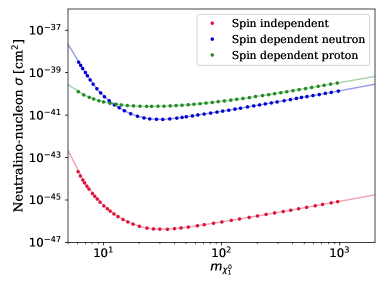
Figure 2: Dark matter direct detection limits in plane of dark matter mass and spin-(in)dependent nucleon scattering cross section. The dots correspond to data extracted from Refs. Aprile:2018dbl ; Aprile:2019dbj , while the solid line is the extrapolation we performed.

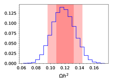
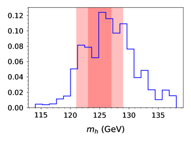
Figure 3: Distribution of the Higgs mass and dark matter relic density predictions, normalised to one. The $1\sigma$ ($2\sigma$) region is marked in red (light red). The MCMC displays an approximate Gaussian fit around the experimental values.

Having implemented and executed the above, 197 chains were recovered. As the parameter space was so vast and such a large number of very precise constraints were used, the efficiency of these scans was very low, requiring weeks of computer time to complete. Therefore, the scans were allowed 2000 Markov chain steps each. After this process we collect the data and applied a likelihood cutoff such that only points with relatively high likelihood are left in the final data set. This was in order to prevent the distributions presented here-in from misleading the reader into thinking some parts of parameter space were viable when, in fact, they produce excessively low likelihoods. The likelihood cutoff applied was $10^{-150}$. Although this is tiny, much of the poor likelihood comes from poor convergence of the fermion masses (see discussion in Section 4.1). In general, the remaining constraints converged very well to the observed values. As an example of two constraints, see Figure 3, which shows how the Higgs boson mass and relic density are centered around the expected value.

4 Results

The subsequent results are based on the Markov Chain Monte Carlo (MCMC) study following the methods elucidated previously. Having already presented two illustrative plots showing the constraints used to guide the MCMC, we now present the resultant spectra and phenomena. We begin with a discussion of the fermion masses, mixing, and a general discussion of the model’s success in recreating the Standard Model observables. We then look at the supersymmetric (SUSY) spectrum, the dark matter sector, and further phenomenological results. Finally, we give a discussion of the effects on collider physics and experimental physics more generally.

4.1 Fermion masses and mixing

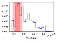
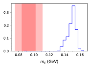
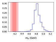
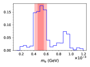
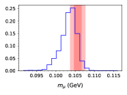
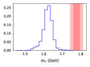
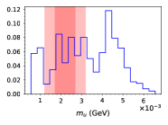
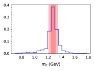
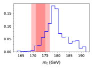
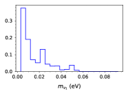
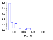
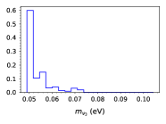
Figure 4: The fermion masses are displayed where the red (light red) region indicating the $1\sigma$ ($2\sigma$) limits. The first generations are very well fitted. However, due to the link between the down type quarks and the leptons at the GUT scale, the second and third generation masses are slightly off. Furthermore, the top mass is also slightly poorly aligned due to the Higgs mass constraint. Note that few points exhibit neutrino masses above the visible part of the histograms.

In this subsection we present the results of our scan for fermion masses and mixing parameters, which are put in as constraints as shown in Table 3. The results for the fermion masses are shown in Figure 4, while those for the mixing parameters are shown in Figures 6 and 7.

These results follow from the charged fermion Yukawa matrices at the GUT scale shown in Eqs. (2.64), together with the neutrino Dirac Yukawa matrix in Eq. (2.66) and the heavy right-handed neutrino mass matrix in Eq. (2.65). Note that the $(3,3)$ entries of the charged lepton and down type quark Yukawa matrices are equal at the GUT scale (yielding approximate bottom-tau unification $m_{b}=m_{s}$), while the $(2,2)$ entries of these matrices differ by the Georgi-Jarlskog (GJ) factor of $3$ (yielding an approximate strange to muon mass ratio $m_{s}=m_{\mu}/3$ at the GUT scale).

The results for fermion masses in Figure 4 show that the above GJ relations do not lead to phenomenologically viable charged lepton and down type quark masses at low energy, in particular $m_{s}$, $m_{b}$ and $m_{\tau}$ are not well fitted. This problem has also been noted by other authors, and possible solutions have been proposed based on various alternative choices of GUT scale Higgs leading to different phenomenologically successful mass ratios at the GUT scale Antusch:2009gu ; Antusch:2013rxa . Since the purpose of this paper is to perform a comprehensive phenomenological analysis on an existing benchmark model, we shall not consider such alternative solutions here, but simply note that such solutions exist and could be readily applied.

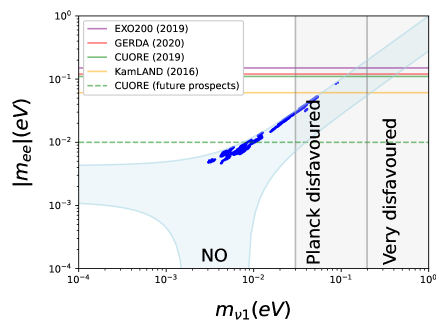
Figure 5: The dark blue points are the model prediction of the neutrinoless double beta decay parameter $|m_{ee}|$ vs the mass of the lightest neutrino $m_{\nu 1}$. The light blue shaded region shows the allowed range in this plane for a normal hierarchy as predicted by the model. The vertical grey shaded bands to the right show the current Planck disfavoured region Planck:2018vyg , while the coloured horizontal lines show the limits on $|m_{ee}|$ from KamLAND KamLAND-Zen:2016pfg , EXO-200 EXO-200:2019rkq , CUORE CUORE:2019yfd , and GERDA GERDA:2020xhi . We also indicate future prospects for CUORE CUORE:2017fp .

Note that the absolute values of the neutrino masses in Figure 4 are genuine predictions of the model, since only the experimentally measured mass squared differences in Table 3 were put in as constraints. In particular, the lightest neutrino mass distribution is peaked around a few times $10^{-3}$ eV. This leads to an interesting prediction for neutrinoless double-beta becay. In Figure 5 we give the model prediction of the neutrinoless double-beta decay parameter $m_{ee}$ against the mass of the lightest neutrino $m_{\nu 1}$. $m_{ee}$ is given by

$$|m_{ee}|=|\sum_{i=1}^{3}{U_{1i}}^{2}m_{\nu i}|\,,$$ (4.75)

where $m_{\nu i}$ are the light neutrino masses and $U$ is the PMNS matrix including the Majorana phases. We use the same convention as in Ref. Zyla:2020zbs . Future projections for CUORE rule out approximately $52\%$ of the data set. Indeed, the model tends to favour relatively high values of $m_{ee}$ as compared to the theoretically allowed region.

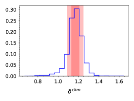
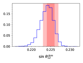
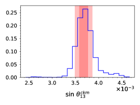
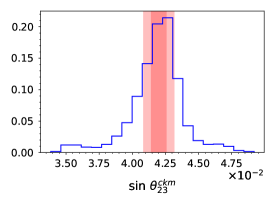
Figure 6: The CKM parameters are displayed where the red (light red) region indicating the $1\sigma$ ($2\sigma$) limits. All parameters in the CKM are fitted very well with an approximately Gaussian distribution around the expected value.

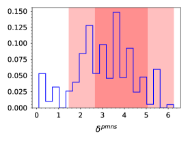
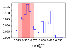
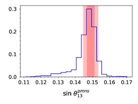
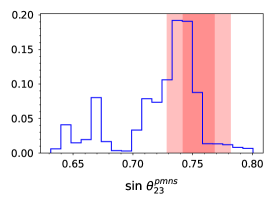
Figure 7: The PMNS parameters are displayed where the red (light red) region indicating the $1\sigma$ ($2\sigma$) limits. Unlike the CKM parameters, the PMNS shows more variation due to the less stringent experimental constraints.

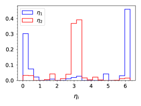
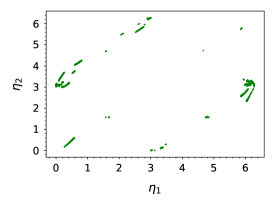
Figure 8: A representation of the Majorana phases is presented. The first panel shows the density of values for the two phases while the second shows their strong correlations.

The results for the CKM and PMNS mixing parameters in Figures 6 and 7 show a good fit to the constraints. The PMNS mixing parameters $\sin\theta_{12}^{\rm PMNS}$ and $\sin\theta_{13}^{\rm PMNS}$ also fit very well. However the model prefers somewhat smaller values of $\sin\theta_{23}^{\rm PMNS}$, with the $CP$-oscillation phase $\delta^{\rm PMNS}$ being quite uniformly distributed.

The Majorana phases are also predicted and are highly correlated as shown in Figure 8. In principle, the fact that they are correlated is not surprising. The model only depends on two high scale phases, $\theta_{2}^{d}$ and $\theta_{3}^{d}$, and the MCMC has two low scale constraints on the phases from $\delta^{CKM}$ and $\delta^{PMNS}$. Therefore, the high scale phases, who determine the Majorana phases, must be correlated. However, the striking nature of the correlation is surprising. It seems that, roughly speaking, the Majorana phases must sum to a multiple of $\pi$. Of course, these phases are important with regards to $CP$-violating processes but this should suggest that their individual values should be multiples of $\pi$, not their sum. For the time being we leave this puzzle as a comment to be understood in greater detail.

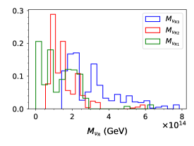
Figure 9: Mass distribution of right handed neutrinos. Overall, the masses are very large and approximately of the same order of magnitude ($10^{14}$ GeV).

4.2 SUSY spectrum

Figure 10 shows the distribution of the lightest charged sfermion masses. We recall from table 1 that in the sfermion sector the $SU(5)$ 5-plets, the first two generation 10-plets and the third generation 10-plet transform as a triplet, doublet and singlet under $S_{4}$, respectively. The nature of the lightest sfermions depens on the mass hierarchy of these states at the GUT scale. In case that $S_{4}$ doublet is the lightest one, then the lightest sfermion consists of a strong admixture of the first two generation sfermions. More precisely, the lightest slepton, $d$-type squark and $u$-type squark will be an admixture of $\tilde{e}_{R}$ and $\tilde{\mu}_{R}$, $\tilde{d}_{L}$ and $\tilde{s}_{L}$, and $\tilde{u}_{R}$ and $\tilde{c}_{R}$, respectively. In all other cases these states will be sfermions of the third generation. On average the corresponding mass splitting is larger in these cases compared to the first one. This can be traced back to the large top Yukawa coupling as well as to a possible difference between the masses of the 10-plet and the 5-plet at the GUT scale.

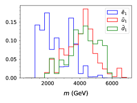
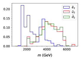
Figure 10: Distribution of masses for the lightest up-type, down-type sfermions and the lightest slepton. The slepton is the lightest of these particles.

The neutralino, chargino, and gluino masses are displayed in Figure 11. Although the gluino mass is not particularly constrained, the two lightest neutralinos and the lightest chargino have a very constrained spectrum. As, a priori, the relic density is too high, the model requires a specific mechanism to reduce the dark matter relic density to phenomenological values. As much of the rest of the spectrum is large, the neutralinos and charginos supply an alternative mechanism via co-annihilation. In order to allow for such contributions, the lightest gauginos must be comparable in mass as will be seen in the dark matter dedicated section below.

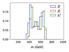
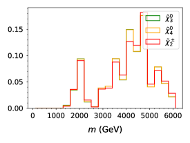
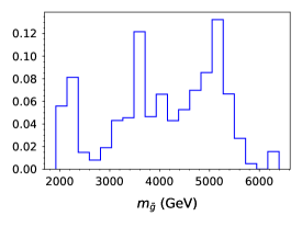
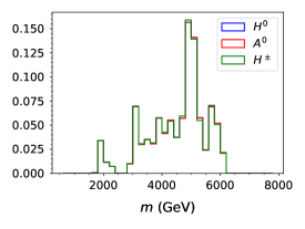
Figure 11: Distribution of the masses of the gauginos and higgses. The mass spectrum of the lightest chargino and two lightest neutralinos is compressed to provide co-annihilation mechanism for dark matter.

The last panel of Figure 11 demonstrates the "decoupling limit" for two Higgs doublet models. In this limit, the three additional Higgs states have very large masses and are approximately degenerate.

Finally, Figure 9 depicts the mass distribution of the heavy neutrinos. Overall, the masses are very large and approximately of the same order of magnitude ($10^{14}$ GeV).

4.3 Dark matter

We now come to the discussion of dark matter aspects of the model under consideration. As we have seen in Figure 3, the dark matter relic density given by the latest Planck results is well accommodated for in the parameter regions surviving the numerous imposed constraints. The corresponding parameter configurations feature essentially bino-like dark matter, which can be understood from Figure 12, where we depict the relevant bino and wino content of the lightest neutralino.

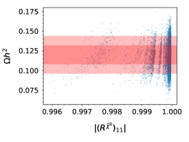
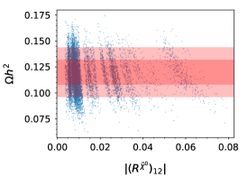
Figure 12: The bino ($|(R^{\tilde{\chi}^{0}})_{11}|$, left) and wino ($|(R^{\tilde{\chi}^{0}})_{12}|$, right) contents of the lightest neutrino shown against the corresponding dark matter relic density. The higgsino contents of the lightest neutralino are negligible and not shown here. The neutralino mixing matrix $R^{\tilde{\chi}^{0}}$ is defined according to the SLHA standard Skands:2003cj . The red (light red) region is indicating the $1\sigma$ ($2\sigma$) limits

Looking at the gaugino masses (Figure 11), it can be seen that the second-lightest neutralino as well as the lighter chargino lie very close to the lightest neutralino. In other words, the bino and wino mass parameters are, at the SUSY scale, almost equal, the bino lying just below the wino mass. This feature is driven by co-annihilations needed to achieve the required relic density. Note that this corresponds to a situation where the GUT-scale values of the bino and wino mass differ roughly by a factor of two.

It is interesting to note that, although the bino-like lightest neutralino $\tilde{\chi}^{0}_{1}$ is the dark matter candidate, the (co-)annihilation cross-section is dominated by the (co-)annihilaton of the wino-like states $\tilde{\chi}^{0}_{2}$ and $\tilde{\chi}^{\pm}$. This is explained, on the one hand, by the very small mass difference between the wino-like states, and, on the other hand, by the enhanced annihilation cross-section for the latter as compared to the bino-like state. Typical final states of these (co-)annihilation channels are quark-antiquark pairs and gauge boson pairs (including $Z^{0}$, $W^{\pm}$, and $\gamma$). Neutrino final states are subdominant.

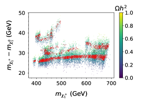
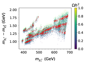
Figure 13: Mass differences between the lightest neutralino (left) as well as the second-lightest neutralino (right) and the lightest neutralino displayed against the lightest chargino mass. Correlations between the masses are displayed with the colour indicating the relic density. In addition, red dots correspond to a relic density of $\Omega h^{2}=0.120\pm 0.006$. The relic density is controlled by co-annihilation channels whose strength are dictated by the mass gap between the relevant particles.

The presence of co-annihilation can also be understood through Figure 13 showing the correlation of the three lightest gaugino masses and the dark matter relic density. Let us finally note that scenarios with wino-like dark matter would give rise to insufficient relic density to align with the experimental evidence, as the wino (co-)annihilation cross-section is numerically more important as the one for the bino.

Coming to the direct dark matter detection, we can see from Figure 14 that this constraint is also well satisfied in the model under consideration, both for the spin-dependent and the spin-independent case. It is important to note that all points shown in Figure 14 lie also below the projected limits of the XENONnT experiment XENON:2020kmp . The fact that all points are found below this limit can be traced to the fact that we have applied a cut on the global likelihood value as explained in Section 3. This procedure discards the points which are too close to the current XENON1T limit, since they typically feature a somewhat lower likelihood value. This means that parameter configurations with reasonably high global likelihood values may not be challenged by direct detection experiments in a near future.

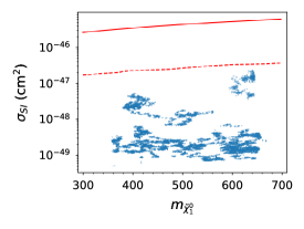
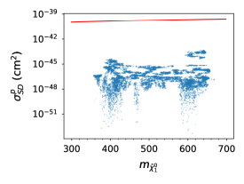
Figure 14: The direct detection limits for spin dependant and spin independent cross-sections are shown with the experimental limit plotted. The solid line indicates the XENON1T limits Aprile:2019dbj , while the dashed line in the first panel indicates the expected limit for the XENONnT XENON:2020kmp experiment. We have precluded a representation of the neutron direct detection calculation as all data points are far away from the exclusion limit, much like the proton calculation of the same.

In summary, the relic density constraint implies a relatively small mass difference between the lightest neutralino and the next-to-lightest states, leading to final states with soft pions and leptons which are difficult to detect. The current bounds depend on the nature of the NLSP go up to masses of about 240 GeV ATLAS:2017vat ; CMS:2018kag ; CMS:2019san ; ATLAS:2019lng . This cuts slightly into the allowed parameter space.

4.4 Collider related aspects

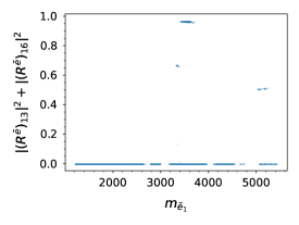
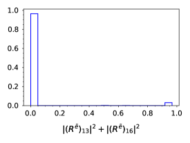
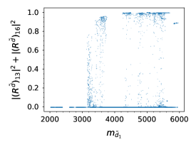
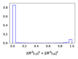
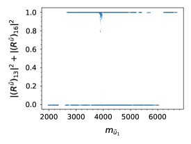
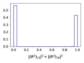
Figure 15: The mass of the lightest sparticle for up and down type squarks and sleptons is plotted against the third generation content for the given particle on the left panels. When the third generation content is close to 0, the sfermion features a second and first generation maximally mixed state. For low mass down squark and slepton states, an admixture of first and second generation is favoured. The right panels illustrate the actual proportion of points that belong to these two extreme flavour cases. The sfermion mixing matrices $R^{\tilde{f}}$ ($\tilde{f}=\tilde{u},\tilde{d},\tilde{e}$) are defined according to the SLHA 2 standard Allanach:2008qq .

As already mentioned in Section 4.2 the flavour structure of the lightest sfermions falls into two extreme case: For each sfermion type, we observe either a first and second generation fully mixed state or a strict third generation state. This feature is illustrated in Figure 15 where we show the distribution of the sum of the square of the mixing matrix entries.

While at first glance it seems that this particular prediction of the model would be quite interesting from a collider perspective, enabling potential flavour mixed search channels, the model also predicts rather high masses for sfermion states. The lightest squark masses are peaked around 4 TeV and stand well beyond any potential collider sensitivity reach (see for e.g. Ref. ATLAS:2020syg where the limits are around 1.8 TeV squarks using simplifying assumptions that do not hold in our case). The lightest slepton on the other hand can be as light as 1 TeV. However, the production cross section drops significantly with respect to the QCD dominated squark ones. Furthermore, our model naturally predicts right-handed slepton states to be the lightest ones which further decreases the production cross section Beenakker:1999xh . As an example, recent searches for flavour conserving channels with nearly helicity degenerated slepton states are excluding masses of the order 600 – 700 GeV ATLAS:2019lff if $m_{\tilde{\chi}^{0}_{1}}<150$ GeV (and limits are even weaker if this is not the case). In addition, current exclusion on $\tau$ flavoured sleptons masses are of order 390 GeV ATLAS:2019gti .

It turns out that our model predictions regarding the sfermionic sector are not very promising for potential collider searches. However this flavour mixing particularity leads to some interesting features from indirect searches perspectives. It is well known that slepton mixing can generate significant contributions to flavour violating decay constraints; in particular, if the mass of the slepton is rather light. In our case, BR$(\mu\rightarrow e\gamma)$ illustrates very well this feature as being one of the most stringent test for lepton flavour violation. Figure 16 shows the distribution of this branching ratio as a function of the mass of the lightest slepton. While the points are within the current experimental limits, it appears that future prospects in the current MEG II experiment MEGII:2018kmf could rule out a vast majority of our light slepton points, implying the interesting conclusion that this particular constraint and other flavour violating constraints would have more discriminatory power than classic direct slepton searches and propose typical smoking guns for our framework. We also note that, while we can have light staus in the model, $\tau\rightarrow e\gamma$ limits are far from constraining our model with branching ratios below $10^{-13}$ while current limits are around $10^{-8}$.

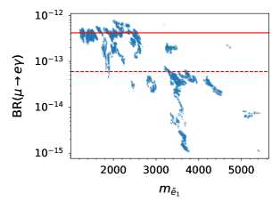
Figure 16: BR$(\mu\rightarrow e\gamma)$ as a function of $m_{\tilde{e}_{1}}$. Current experimental limit is represented by the red solid line while the dashed one corresponds to the future prospects of MEG II ($6\cdot 10^{-14}$) MEGII:2018kmf .

Despite the sfermionic states being unreachable in near future collider searches, this is not necessarily the case for the other SUSY particles in our model. In particular, the model can predict rather light electroweakinos with sufficient mass gap for collider considerations. As a comparison, recent searches from ATLAS ATLAS:2021moa put a lower bound on $m_{\tilde{\chi}_{1}^{0}}$ of 270 GeV when the mass gap with $m_{\tilde{\chi}_{1}^{\pm}}$ is of order 50 GeV. While this very light masses are not present in our current framework, we can hope for more stringent limits from future LHC runs.

Similar conclusion can be derived regarding gluino searches. While the predicted masses lie in the 2 – 6 TeV range, ATLAS and CMS limits using simplified models ATLAS:2020syg ; CMS:2019zmd reaches 1.8 TeV exclusion. Again, we can argue that future LHC runs might restrict our light spectrum parameter distributions.

To illustrate the collider phenomenology we present three benchmark points where relevant information is given in Table 5. The detailed information is added as supplementary material to the arXiv submission of this paper. In particular, we list the masses of the electroweakinos for an illustrative point with low masses for the light gauginos and a relatively small mass gap. We also give the dominant decay channels and decay widths. All other particles are too heavy to be detected in the upcoming LHC run. We give a benchmark for a point which features, besides the light chargino and the neutralinos of BP1, a gluino with mass 2 TeV which should be in reach of the upcoming LHC run. Again, we give the masses, decay widths, and decay channels for the particles under examination. Regarding the third benchmark point, while having similar features as BP2 in view of collider physics, it further highlights the fully mixed nature of the lightest sleptons and the potential relevance for $\mu\to e\gamma$. Its branching of $4\cdot 10^{-13}$ is close to the current experimental bound. However, even if this rare decay is discovered in an upcoming experiment, this example shows that it will be rather challenging to detect lepton flavour at a high energy collider as the sleptons are quite heavy.

	Particle	Mass	Decay Width	Decay Channels	Branching Ratio
BP1	$\tilde{\chi}_{1}$	$402$	$0$
	$\tilde{\chi}_{2}$	$442$	$1.76\times 10^{-11}$	$\tilde{\chi}_{1}\>\bar{q}\>q$ $\tilde{\chi}_{1}\>\bar{b}\>b$ $\tilde{\chi}_{1}\>\nu_{i}\nu_{i}$	70% 13% 14%
	$\tilde{\chi}_{1}^{+}$	$444$	$1.5\times 10^{-8}$	$\tilde{\chi}_{1}\>\bar{q}\>q$ $\tilde{\chi}_{1}\>\bar{l}\>\nu_{i}$	67% 33%
BP2	$\tilde{G}$	$2000$	$1.87\times 10^{-1}$	$\tilde{\chi_{1}}\>\bar{q}\>q$ $\tilde{\chi_{1}^{\pm}}\>q^{*}\>q$ $\tilde{\chi}_{2}\>q^{*}\>q$	11% 46% 35%
BP3	$\tilde{e}_{1}$	$1470$	$6.6$	$\tilde{\chi}_{1}\>e$ $\tilde{\chi}_{1}\>\mu$	44% 56%
	$\tilde{e}_{2}$	$1500$	$6.8$	$\tilde{\chi}_{1}\>e$ $\tilde{\chi}_{1}\>\mu$	56% 44%
	$\tilde{\chi}_{1}$	$413$	$0$
	$\tilde{\chi}_{2}$	$439$	$3.72\times 10^{-11}$	$\tilde{\chi}_{1}\>q^{*}\>q$ $\tilde{\chi}_{1}\>\nu\>\nu$	81% 15%
	$\tilde{\chi}_{1}^{+}$	$440$	$5.18\times 10^{-8}$	$\tilde{\chi}_{1}\>q^{*}\>q$ $\tilde{\chi}_{1}\>\nu\>e^{*}$	67% 33%
	$\tilde{G}$	$2110$	$0.228$	$\tilde{\chi}_{1}\>q^{*}\>q$ $\tilde{\chi}_{1}^{\pm}\>q^{*}\>q$ $\tilde{\chi}_{2}\>q^{*}\>q$	13% 50% 37%

Table 5: Selected benchmark points (BP) for phenomenology. The first BP exhibits rather light electroweakinos and might represent a challenge for future colliders. The second BP has a rather light gluino, which is already close to the current experimental limits from the LHC collaborations. Finally, the last BP is an example of maximally mixed lightest sleptons. All masses and widths are given in GeV.

5 Conclusion

In this paper we have presented a detailed phenomenological analysis of a concrete Supersymmetric (SUSY) Grand Unified Theory (GUT) of flavour, based on $SU(5)\times S_{4}$. The model predicts charged fermion and neutrino mass and mixing, and where the mass matrices of both the Standard Model and the Supersymmetric particles are controlled by a common symmetry at the GUT scale, with only two input phases. The considered framework predicts small but non-vanishing non-minimal flavour violating effects, motivating a sophisticated data-driven parameter analysis to uncover the signatures and viability of the model.

The computer-intensive Markov-Chain-Monte-Carlo (MCMC) based analysis performed here, the first of its kind to include a large range of flavour as well as dark matter and SUSY observables, predicts distributions for a range of physical quantities which may be used to test the model. The predictions include maximally mixed sfermions, $\mu\rightarrow e\gamma$ close to its experimental limit and successful bino-like dark matter with nearby winos (making direct detection unlikely), implying good prospects for discovering winos and gluinos at forthcoming collider runs. The results also demonstrate that the Georgi-Jarlskog mechanism does not provide a good description of the splitting of down type quark masses and charged leptons. However neutrinoless double beta decay, which depends on a curious pattern of Majorana phases resulting from the two input phases, is predicted at observable rates.

The analysis here may be repeated for any given SUSY GUT of flavour, leading to corresponding predictions for fermion masses and mixing as well as SUSY masses and flavour violating physical observables at colliders and high precision experiments. The results here exemplify the synergy between the theory of quark and lepton (including neutrino) mass and mixing, dark matter and the SUSY particle spectrum and flavour violation, that is possible within such frameworks. It is only by systematically confronting the detailed predictions of concrete examples of SUSY GUTs of flavour with experiment that the underlying unified theory of quark and lepton flavour beyond the Standard Model may eventually be discovered.

Appendix A SPheno

Our results have been obtained using the numerical code SPheno Porod:2003um ; Porod:2011nf , where we have implemented the model using SARAH v4.14.0 Staub:2008uz ; Staub:2013tta ; Staub:2012pb ; Staub:2010jh ; Staub:2009bi and then adapted the code for the model at hand. Here we describe the corresponding modifications.

In the standard version of SPheno the SM fermion masses, the CKM matrix, the mass of the $Z$-boson $m_{Z}$, the Fermi constant, the electromagnetic coupling $\alpha$, and the strong coupling $\alpha_{s}(m_{Z})$ serve as input. The latter can either be given in the Thomson limit or in the $\overline{\rm MS}$-scheme at $Q=m_{Z}$. From these the three gauge couplings, the SM vacuum expectation value (VEV) $v$ of the Higgs boson and the Yukawa couplings are calculated at the scale $Q=m_{Z}$. The couplings are then evolved up to the scale $M_{\rm SUSY}$ where the SM and the MSSM are matched including one-loop SUSY threshold corrections.

In the model at hand the Yukawa couplings are given at the GUT-scale and the fermion masses, the CKM-matrix and the PMNS-matrix are an output which required some changes to the code. The input which is done via the standard SUSY Les Houches format Skands:2003cj ; Allanach:2008qq with the slight modification that the Yukawa couplings can be input at the GUT scale. The input is given at different scales as follows:

• at $M_{\rm GUT}$: $Y_{\ell}$, $Y_{\nu}$, $Y_{d}$, $Y_{u}$, arg($\mu$) (in practice the sign of $\mu$), as well as the soft SUSY breking terms in a non-universal form: scalar mass squares $m^{2}_{\tilde{f}}$ ($\tilde{f}=\dots$), trilinear couplings $A_{\tilde{f}}$ ($\tilde{f}=\dots$) and non-universal gaugino mass parameters $M_{1}$, $M_{2}$, $M_{3}$. All phases can be non-zero in principle.

• at $M_{\rm SUSY}$: $\tan\beta$

• at $Q=m_{Z}$: $G_{F}$, $m_{Z}$, $\alpha_{s}$, $\alpha_{em}(m_{Z})$

The calculation is done in an iterative way:

1. The gauge couplings are evolved from the electroweak scale using the SUSY RGEs at the one-loop level to $M_{\rm GUT}=2\cdot 10^{16}$ GeV. We do not require unification at this scale. These couplings at this stage serve only as a starting point for our iteration.

2. All parameters are evolved from $M_{\rm GUT}$ to $M_{\rm SUSY}=\sqrt{(M_{Q})_{33}(M_{U})_{33}}$ using RGEs at the two-loop level. The right-handed neutrinos are decoupled at their respective mass scale during this evaluation and the contributions to the Weinberg operator are calculated at these scales as well. The running of this operator is taken into account as well.

3. The SUSY spectrum is calculated at the scale $M_{\rm SUSY}$ at the one-loop level and the heavy Higgs masses at two-loop level taking into account the contributions from third generation sfermions and fermions, see Ref. Slavich:2020zjv for a summary. In addition the matching to the SM-parameters is performed as described in Ref. Staub:2017jnp .

4. The SM-parameters are evolved from $M_{\rm SUSY}$ to $m_{Z}$ using the two-loop SM RGEs. At $m_{Z}$, the masses of the SM fermions are calculated and the mass of the Higgs boson at the two-loop level. For these calculations we however take $G_{F}$, $m_{Z}$, $\alpha(m_{Z})$ and $\alpha_{s}(m_{Z})$ to calculate the gauge couplings and the VEV.

5. The gauge and Yukawa couplings as well as the quartic Higgs couplings are then evolved to $M_{\rm SUSY}$ using the two-loop RGEs. At this scale the SUSY threshold corrections to the gauge and Yukawa couplings are taken into account. The resulting couplings are evolved to $M_{\rm GUT}=2\cdot 10^{16}$ GeV. Then steps 2. to 4. are repeated until a relative precision of all masses at the level of $10^{-5}$ is reached.

6. Once the precision goal for the spectrum has been achieved, the flavour observables are calculated. Also here we have modified the procedure slightly: we have a quite heavy spectrum leading potentially large logs of the form $\ln(M_{\rm SUSY}/m_{t})$. For this reason the calculation is done in two steps: (i) Calculate the SUSY contributions to the Wilson coefficients at $Q=M_{\rm SUSY}$. (ii) Calculate the SM contributions to the Wilson coefficients at $Q=m_{t}$. (iii) Add both contributions to calculate the relevant observables.

References

- (1) ATLAS Collaboration, G. Aad et al., Observation of a new particle in the search for the Standard Model Higgs boson with the ATLAS detector at the LHC, Phys. Lett. B716 (2012) 1–29, [arXiv:1207.7214].
- (2) CMS Collaboration, S. Chatrchyan et al., Observation of a new boson at a mass of 125 GeV with the CMS experiment at the LHC, Phys. Lett. B716 (2012) 30–61, [arXiv:1207.7235].
- (3) P. Minkowski, at a Rate of One Out of 1-Billion Muon Decays?, Phys.Lett. B67 (1977) 421.
- (4) M. Gell-Mann, P. Ramond, and R. Slansky, Complex Spinors and Unified Theories, Conf.Proc. C790927 (1979) 315–321, [arXiv:1306.4669].
- (5) T. Yanagida, Horizontal Symmetry and Masses of Neutrinos, Conf.Proc. C7902131 (1979) 95–99.
- (6) R. N. Mohapatra and G. Senjanovic, Neutrino Mass and Spontaneous Parity Violation, Phys.Rev.Lett. 44 (1980) 912.
- (7) J. Schechter and J. W. F. Valle, Neutrino Masses in Theories, Phys. Rev. D22 (1980) 2227.
- (8) N. Cabibbo, Unitary Symmetry and Leptonic Decays, Phys. Rev. Lett. 10 (1963) 531–533.
- (9) M. Kobayashi and T. Maskawa, CP Violation in the Renormalizable Theory of Weak Interaction, Prog. Theor. Phys. 49 (1973) 652–657.
- (10) Z. Maki, M. Nakagawa, and S. Sakata, Remarks on the unified model of elementary particles, Prog. Theor. Phys. 28 (1962) 870–880.
- (11) B. Pontecorvo, Neutrino Experiments and the Problem of Conservation of Leptonic Charge, Sov. Phys. JETP 26 (1968) 984–988. [Zh. Eksp. Teor. Fiz.53,1717(1967)].
- (12) M. Arana-Catania, S. Heinemeyer, and M. J. Herrero, Updated Constraints on General Squark Flavor Mixing, Phys. Rev. D 90 (2014), no. 7 075003, [arXiv:1405.6960].
- (13) K. Kowalska, Phenomenology of SUSY with General Flavour Violation, JHEP 09 (2014) 139, [arXiv:1406.0710].
- (14) K. De Causmaecker, B. Fuks, B. Herrmann, F. Mahmoudi, B. O’Leary, W. Porod, S. Sekmen, and N. Strobbe, General squark flavour mixing: constraints, phenomenology and benchmarks, JHEP 11 (2015) 125, [arXiv:1509.05414].
- (15) A. Bartl, K. Hidaka, K. Hohenwarter-Sodek, T. Kernreiter, W. Majerotto, and W. Porod, Test of lepton flavor violation at LHC, Eur. Phys. J. C 46 (2006) 783–789, [hep-ph/0510074].
- (16) G. Bozzi, B. Fuks, B. Herrmann, and M. Klasen, Squark and gaugino hadroproduction and decays in non-minimal flavour violating supersymmetry, Nucl. Phys. B 787 (2007) 1–54, [arXiv:0704.1826].
- (17) A. Bartl, K. Hidaka, K. Hohenwarter-Sodek, T. Kernreiter, W. Majerotto, and W. Porod, Impact of slepton generation mixing on the search for sneutrinos, Phys. Lett. B 660 (2008) 228–235, [arXiv:0709.1157].
- (18) F. del Aguila et al., Collider aspects of flavour physics at high , Eur. Phys. J. C 57 (2008) 183–308, [arXiv:0801.1800].
- (19) T. Hurth and W. Porod, Flavour violating squark and gluino decays, JHEP 08 (2009) 087, [arXiv:0904.4574].
- (20) A. Bartl, K. Hidaka, K. Hohenwarter-Sodek, T. Kernreiter, W. Majerotto, and W. Porod, Impact of squark generation mixing on the search for gluinos at LHC, Phys. Lett. B 679 (2009) 260–266, [arXiv:0905.0132].
- (21) M. Bruhnke, B. Herrmann, and W. Porod, Signatures of bosonic squark decays in non-minimally flavour-violating supersymmetry, JHEP 09 (2010) 006, [arXiv:1007.2100].
- (22) A. Bartl, H. Eberl, B. Herrmann, K. Hidaka, W. Majerotto, and W. Porod, Impact of squark generation mixing on the search for squarks decaying into fermions at LHC, Phys. Lett. B 698 (2011) 380–388, [arXiv:1007.5483]. [Erratum: Phys.Lett.B 700, 390–390 (2011)].
- (23) A. Bartl, H. Eberl, E. Ginina, B. Herrmann, K. Hidaka, W. Majerotto, and W. Porod, Flavour violating gluino three-body decays at LHC, Phys. Rev. D 84 (2011) 115026, [arXiv:1107.2775].
- (24) A. Bartl, H. Eberl, E. Ginina, B. Herrmann, K. Hidaka, W. Majerotto, and W. Porod, Flavor violating bosonic squark decays at LHC, Int. J. Mod. Phys. A 29 (2014), no. 07 1450035, [arXiv:1212.4688].
- (25) A. Bartl, H. Eberl, E. Ginina, K. Hidaka, and W. Majerotto, as a test case for quark flavor violation in the MSSM, Phys. Rev. D 91 (2015), no. 1 015007, [arXiv:1411.2840].
- (26) M. Blanke, B. Fuks, I. Galon, and G. Perez, Gluino Meets Flavored Naturalness, JHEP 04 (2016) 044, [arXiv:1512.03813].
- (27) G. Brooijmans et al., Les Houches 2017: Physics at TeV Colliders New Physics Working Group Report, in 10th Les Houches Workshop on Physics at TeV Colliders, 3, 2018. arXiv:1803.10379.
- (28) A. Chakraborty, M. Endo, B. Fuks, B. Herrmann, M. M. Nojiri, P. Pani, and G. Polesello, Flavour-violating decays of mixed top-charm squarks at the LHC, Eur. Phys. J. C 78 (2018), no. 10 844, [arXiv:1808.07488].
- (29) V. Barger, D. Marfatia, A. Mustafayev, and A. Soleimani, SUSY dark matter and lepton flavor violation, Phys. Rev. D 80 (2009) 076004, [arXiv:0908.0941].
- (30) D. Choudhury, R. Garani, and S. K. Vempati, Flavored Co-annihilations, JHEP 06 (2012) 014, [arXiv:1104.4467].
- (31) B. Herrmann, M. Klasen, and Q. Le Boulc’h, Impact of squark flavour violation on neutralino dark matter, Phys. Rev. D 84 (2011) 095007, [arXiv:1106.6229].
- (32) P. Agrawal, M. Blanke, and K. Gemmler, Flavored dark matter beyond Minimal Flavor Violation, JHEP 10 (2014) 072, [arXiv:1405.6709].
- (33) U. Amaldi, W. de Boer, and H. Furstenau, Comparison of grand unified theories with electroweak and strong coupling constants measured at LEP, Phys. Lett. B 260 (1991) 447–455.
- (34) A. S. Belyaev, S. F. King, and P. B. Schaefers, Muon g-2 and dark matter suggest nonuniversal gaugino masses: case study at the LHC, Phys. Rev. D97 (2018), no. 11 115002, [arXiv:1801.00514].
- (35) M. Dimou, S. F. King, and C. Luhn, Phenomenological implications of an SU(5)S4 U(1) SUSY GUT of flavor, Phys. Rev. D93 (2016), no. 7 075026, [arXiv:1512.09063].
- (36) M. Dimou, S. F. King, and C. Luhn, Approaching Minimal Flavour Violation from an SUSY GUT, JHEP 02 (2016) 118, [arXiv:1511.07886].
- (37) J. Bernigaud, B. Herrmann, S. F. King, and S. J. Rowley, Non-minimal flavour violation in A SU(5) SUSY GUTs with smuon assisted dark matter, JHEP 03 (2019) 067, [arXiv:1812.07463].
- (38) K. Mukaida, K. Schmitz, and M. Yamada, Leptoflavorgenesis: baryon asymmetry of the Universe from lepton flavor violation, arXiv:2111.03082.
- (39) N. Metropolis, A. W. Rosenbluth, M. N. Rosenbluth, A. H. Teller, and E. Teller, Equation of state calculations by fast computing machines, J. Chem. Phys. 21 (1953) 1087–1092.
- (40) W. K. Hastings, Monte Carlo Sampling Methods Using Markov Chains and Their Applications, Biometrika 57 (1970) 97–109.
- (41) A. A. Markov, Extension of the limit theorems of probability theory to a sum of variables connected in a chain. reprinted in Appendix B of: R. Howard, Dynamic Probabilistic Systems, volume 1: Markov Chains, John Wiley and Sons, 1971.
- (42) C. Hagedorn, S. F. King, and C. Luhn, A SUSY GUT of Flavour with S4 x SU(5) to NLO, JHEP 06 (2010) 048, [arXiv:1003.4249].
- (43) C. Hagedorn, S. F. King, and C. Luhn, SUSY S SU(5) revisited, Phys. Lett. B717 (2012) 207–213, [arXiv:1205.3114].
- (44) D. J. H. Chung, L. L. Everett, G. L. Kane, S. F. King, J. D. Lykken, and L.-T. Wang, The Soft supersymmetry breaking Lagrangian: Theory and applications, Phys. Rept. 407 (2005) 1–203, [hep-ph/0312378].
- (45) L. Wolfenstein, Parametrization of the Kobayashi-Maskawa Matrix, Phys. Rev. Lett. 51 (1983) 1945.
- (46) C. Luhn, Trimaximal TM1 neutrino mixing in S4 with spontaneous CP violation, Nucl. Phys. B875 (2013) 80–100, [arXiv:1306.2358].
- (47) R. Gatto, G. Sartori, and M. Tonin, Weak Selfmasses, Cabibbo Angle, and Broken , Phys. Lett. 28B (1968) 128–130.
- (48) H. Georgi and C. Jarlskog, A New Lepton - Quark Mass Relation in a Unified Theory, Phys. Lett. 86B (1979) 297–300.
- (49) S. Antusch and M. Spinrath, New GUT predictions for quark and lepton mass ratios confronted with phenomenology, Phys. Rev. D 79 (2009) 095004, [arXiv:0902.4644].
- (50) S. Antusch, S. F. King, and M. Spinrath, GUT predictions for quark-lepton Yukawa coupling ratios with messenger masses from non-singlets, Phys. Rev. D 89 (2014), no. 5 055027, [arXiv:1311.0877].
- (51) S. F. King, J. P. Roberts, and D. P. Roy, Natural dark matter in SUSY GUTs with non-universal gaugino masses, JHEP 10 (2007) 106, [arXiv:0705.4219].
- (52) F. Staub, SARAH, arXiv:0806.0538.
- (53) F. Staub, SARAH 4 : A tool for (not only SUSY) model builders, Comput. Phys. Commun. 185 (2014) 1773–1790, [arXiv:1309.7223].
- (54) F. Staub, SARAH 3.2: Dirac Gauginos, UFO output, and more, Comput. Phys. Commun. 184 (2013) 1792–1809, [arXiv:1207.0906].
- (55) F. Staub, Automatic Calculation of supersymmetric Renormalization Group Equations and Self Energies, Comput. Phys. Commun. 182 (2011) 808–833, [arXiv:1002.0840].
- (56) F. Staub, From Superpotential to Model Files for FeynArts and CalcHep/CompHep, Comput. Phys. Commun. 181 (2010) 1077–1086, [arXiv:0909.2863].
- (57) W. Porod, SPheno, a program for calculating supersymmetric spectra, SUSY particle decays and SUSY particle production at colliders, Comput. Phys. Commun. 153 (2003) 275–315, [hep-ph/0301101].
- (58) W. Porod and F. Staub, SPheno 3.1: Extensions including flavour, CP-phases and models beyond the MSSM, Comput. Phys. Commun. 183 (2012) 2458–2469, [arXiv:1104.1573].
- (59) W. Porod, F. Staub, and A. Vicente, A Flavor Kit for BSM models, Eur. Phys. J. C 74 (2014), no. 8 2992, [arXiv:1405.1434].
- (60) M. D. Goodsell, K. Nickel, and F. Staub, Two-Loop Higgs mass calculations in supersymmetric models beyond the MSSM with SARAH and SPheno, Eur. Phys. J. C 75 (2015), no. 1 32, [arXiv:1411.0675].
- (61) M. Goodsell, K. Nickel, and F. Staub, Generic two-loop Higgs mass calculation from a diagrammatic approach, Eur. Phys. J. C 75 (2015), no. 6 290, [arXiv:1503.03098].
- (62) M. D. Goodsell and F. Staub, The Higgs mass in the CP violating MSSM, NMSSM, and beyond, Eur. Phys. J. C 77 (2017), no. 1 46, [arXiv:1604.05335].
- (63) J. Braathen, M. D. Goodsell, and F. Staub, Supersymmetric and non-supersymmetric models without catastrophic Goldstone bosons, Eur. Phys. J. C 77 (2017), no. 11 757, [arXiv:1706.05372].
- (64) P. Z. Skands et al., SUSY Les Houches accord: Interfacing SUSY spectrum calculators, decay packages, and event generators, JHEP 07 (2004) 036, [hep-ph/0311123].
- (65) B. C. Allanach et al., SUSY Les Houches Accord 2, Comput. Phys. Commun. 180 (2009) 8–25, [arXiv:0801.0045].
- (66) Particle Data Group Collaboration, P. Zyla et al., Review of Particle Physics, PTEP 2020 (2020), no. 8 083C01.
- (67) I. Esteban, M. C. Gonzalez-Garcia, A. Hernandez-Cabezudo, M. Maltoni, and T. Schwetz, Global analysis of three-flavour neutrino oscillations: synergies and tensions in the determination of , , and the mass ordering, JHEP 01 (2019) 106, [arXiv:1811.05487].
- (68) “Unitarity triangle fit.” http://www.utfit.org/UTfit/WebHome. Accessed: 2020-02-03.
- (69) Planck Collaboration, P. A. R. Ade et al., Planck 2015 results. XIII. Cosmological parameters, Astron. Astrophys. 594 (2016) A13, [arXiv:1502.01589].
- (70) G. Bélanger, F. Boudjema, A. Pukhov, and A. Semenov, MicrOMEGAs: A Program for calculating the relic density in the MSSM, Comput. Phys. Commun. 149 (2002) 103–120, [hep-ph/0112278].
- (71) G. Bélanger, F. Boudjema, A. Pukhov, and A. Semenov, micrOMEGAs: Version 1.3, Comput. Phys. Commun. 174 (2006) 577–604, [hep-ph/0405253].
- (72) D. Barducci, G. Belanger, J. Bernon, F. Boudjema, J. Da Silva, S. Kraml, U. Laa, and A. Pukhov, Collider limits on new physics within micrOMEGAs_4.3, Comput. Phys. Commun. 222 (2018) 327–338, [arXiv:1606.03834].
- (73) XENON Collaboration, E. Aprile et al., Dark Matter Search Results from a One Ton-Year Exposure of XENON1T, Phys. Rev. Lett. 121 (2018), no. 11 111302, [arXiv:1805.12562].
- (74) XENON Collaboration, E. Aprile et al., Constraining the spin-dependent WIMP-nucleon cross sections with XENON1T, Phys. Rev. Lett. 122 (2019), no. 14 141301, [arXiv:1902.03234].
- (75) P. Slavich et al., Higgs-mass predictions in the MSSM and beyond, Eur. Phys. J. C 81 (2021), no. 5 450, [arXiv:2012.15629].
- (76) Planck Collaboration, N. Aghanim et al., Planck 2018 results. VI. Cosmological parameters, Astron. Astrophys. 641 (2020) A6, [arXiv:1807.06209]. [Erratum: Astron.Astrophys. 652, C4 (2021)].
- (77) KamLAND-Zen Collaboration, A. Gando et al., Search for Majorana Neutrinos near the Inverted Mass Hierarchy Region with KamLAND-Zen, Phys. Rev. Lett. 117 (2016), no. 8 082503, [arXiv:1605.02889]. [Addendum: Phys.Rev.Lett. 117, 109903 (2016)].
- (78) EXO-200 Collaboration, G. Anton et al., Search for Neutrinoless Double- Decay with the Complete EXO-200 Dataset, Phys. Rev. Lett. 123 (2019), no. 16 161802, [arXiv:1906.02723].
- (79) CUORE Collaboration, D. Q. Adams et al., Improved Limit on Neutrinoless Double-Beta Decay in 130Te with CUORE, Phys. Rev. Lett. 124 (2020), no. 12 122501, [arXiv:1912.10966].
- (80) GERDA Collaboration, M. Agostini et al., Final Results of GERDA on the Search for Neutrinoless Double- Decay, Phys. Rev. Lett. 125 (2020), no. 25 252502, [arXiv:2009.06079].
- (81) L. Canonica et al., Status and prospects for CUORE, J. Phys. Conf. Ser. 888 (2017), no. 1 012034.
- (82) XENON Collaboration, E. Aprile et al., Projected WIMP sensitivity of the XENONnT dark matter experiment, JCAP 11 (2020) 031, [arXiv:2007.08796].
- (83) ATLAS Collaboration, M. Aaboud et al., Search for electroweak production of supersymmetric states in scenarios with compressed mass spectra at TeV with the ATLAS detector, Phys. Rev. D 97 (2018), no. 5 052010, [arXiv:1712.08119].
- (84) CMS Collaboration, A. M. Sirunyan et al., Search for new physics in events with two soft oppositely charged leptons and missing transverse momentum in proton-proton collisions at 13 TeV, Phys. Lett. B 782 (2018) 440–467, [arXiv:1801.01846].
- (85) CMS Collaboration, A. M. Sirunyan et al., Search for supersymmetry with a compressed mass spectrum in the vector boson fusion topology with 1-lepton and 0-lepton final states in proton-proton collisions at 13 TeV, JHEP 08 (2019) 150, [arXiv:1905.13059].
- (86) ATLAS Collaboration, G. Aad et al., Searches for electroweak production of supersymmetric particles with compressed mass spectra in 13 TeV collisions with the ATLAS detector, Phys. Rev. D 101 (2020), no. 5 052005, [arXiv:1911.12606].
- (87) ATLAS Collaboration, G. Aad et al., Search for squarks and gluinos in final states with jets and missing transverse momentum using 139 fb-1 of =13 TeV collision data with the ATLAS detector, JHEP 02 (2021) 143, [arXiv:2010.14293].
- (88) W. Beenakker, M. Klasen, M. Kramer, T. Plehn, M. Spira, and P. M. Zerwas, The Production of charginos / neutralinos and sleptons at hadron colliders, Phys. Rev. Lett. 83 (1999) 3780–3783, [hep-ph/9906298]. [Erratum: Phys.Rev.Lett. 100, 029901 (2008)].
- (89) ATLAS Collaboration, G. Aad et al., Search for electroweak production of charginos and sleptons decaying into final states with two leptons and missing transverse momentum in TeV collisions using the ATLAS detector, Eur. Phys. J. C 80 (2020), no. 2 123, [arXiv:1908.08215].
- (90) ATLAS Collaboration, G. Aad et al., Search for direct stau production in events with two hadronic -leptons in TeV collisions with the ATLAS detector, Phys. Rev. D 101 (2020), no. 3 032009, [arXiv:1911.06660].
- (91) MEG II Collaboration, A. M. Baldini et al., The design of the MEG II experiment, Eur. Phys. J. C 78 (2018), no. 5 380, [arXiv:1801.04688].
- (92) ATLAS Collaboration, G. Aad et al., Search for chargino–neutralino pair production in final states with three leptons and missing transverse momentum in TeV collisions with the ATLAS detector, arXiv:2106.01676.
- (93) CMS Collaboration, A. M. Sirunyan et al., Search for supersymmetry in proton-proton collisions at 13 TeV in final states with jets and missing transverse momentum, JHEP 10 (2019) 244, [arXiv:1908.04722].
- (94) F. Staub and W. Porod, Improved predictions for intermediate and heavy Supersymmetry in the MSSM and beyond, Eur. Phys. J. C 77 (2017), no. 5 338, [arXiv:1703.03267].