Temporally Consistent Online Depth Estimation in Dynamic Scenes
Abstract
Temporally consistent depth estimation is crucial for online applications such as augmented reality. While stereo depth estimation has received substantial attention as a promising way to generate 3D information, there is relatively little work focused on maintaining temporal stability. Indeed, based on our analysis, current techniques still suffer from poor temporal consistency. Stabilizing depth temporally in dynamic scenes is challenging due to concurrent object and camera motion. In an online setting, this process is further aggravated because only past frames are available. We present a framework named Consistent Online Dynamic Depth (CODD) to produce temporally consistent depth estimates in dynamic scenes in an online setting. CODD augments per-frame stereo networks with novel motion and fusion networks. The motion network accounts for dynamics by predicting a per-pixel SE3 transformation and aligning the observations. The fusion network improves temporal depth consistency by aggregating the current and past estimates. We conduct extensive experiments and demonstrate quantitatively and qualitatively that CODD outperforms competing methods in terms of temporal consistency and performs on par in terms of per-frame accuracy. Project page: https://mli0603.github.io/codd
1 Introduction
[loop,controls=play,width=]6img/animation/frame_2561
For online applications such as augmented reality, estimating consistent depth across video sequences is important, as temporal noise in depth estimation may corrupt visual quality and interfere with downstream processing such as surface extraction. One way to acquire metric depth (i.e. without scale ambiguity) is to use calibrated stereo images. Recent developments in stereo depth estimation have been focusing on improving disparity accuracy on a per-frame basis [9, 4, 7, 30, 16]. However, none of these approaches considers temporal information nor attempts to maintain temporal consistency. We examine the temporal stability of different per-frame networks and find that current solutions suffer from poor temporal consistency. We quantify such temporal inconsistency in predictions in Sect. 4 and provide qualitative visualization of resulting artifacts in the video supplement to further illustrate the case.
We posit that stabilizing depth estimation temporally requires reasoning between current and previous frames, i.e. establishing cross-frame correspondences and correlating the predicted values. In the simplest case where the scene is entirely static and camera poses are known [18, 19], camera motion can be corrected by a single SE3 transformation. Considering geometric constraints of multiple camera views [1], the aligned cameras have the same viewpoint onto the static scene and therefore, depth values are expected to be the same, which allows pixel-wise aggregation of depth estimates from different times for consistency.
However, in a dynamic environment with moving and deforming objects, multi-view constraints do not hold. Even if cross-frame correspondences are established, independent depth estimates for corresponding points cannot simply be fused. This is because depth is not translation invariant and thus, fusion requires aligning depth predictions into a common coordinate frame. Therefore, prior works [21, 15] explicitly remove moving objects and only stabilize the static background to comply with the constraint. Given additional 3D motion, e.g. estimated by scene flow, the depth of both moving and static objects can be aligned, which then enables temporal consistency processing [41]. However, as do the previously mentioned approaches, Zhang et al. [41] use information from all video frames and optimize network parameters at application time, limiting itself to offline use.
In an online setting, prior works [29, 40, 6] incorporate temporal information by appending a recurrent network to the depth estimation modules. However, these recurrent networks do not provide explicit reasoning between frames. Moreover, these approaches [29, 40, 6] consider depth estimation from single images, not stereo pairs. Due to the scale ambiguity of monocular depth estimation, prior works mainly focus on producing estimates with consistent scale [15, 41] instead of reducing the inter-frame jitter that arises in metric depth estimation.
Traditionally, to encourage temporal consistency in metric depth, prior techniques have relied on hand-crafted probability weights [13, 23, 33]. One example is the Kalman filter [13], which combines previous and current predictions based on associated uncertainties. However, it assumes Gaussian measurement error, which often fails in scenarios with occlusion and de-occlusion between frames.
We present a framework named Consistent Online Dynamic Depth (CODD) that produces temporally consistent depth predictions. To account for inter-frame motion, we integrate a motion network that predicts a per-pixel SE3 transformation that aligns previous estimates to the current frame. To remove temporal jitters and outliers from estimates, a fusion network is designed to aggregate depth predictions temporally. Compared with existing methods, CODD produces temporally consistent metric depth and is capable of handling dynamic scenes in an online setting. Qualitative results of improved temporal consistency of CODD framework are shown in Fig. 1.
For evaluation, we first show empirically that current stereo depth estimation solutions indeed suffer from poor temporal stability. We quantify such inconsistency with a set of temporal metrics and find that networks with better per-frame accuracy may have worse temporal consistency. We then benchmark CODD on varied datasets, including synthetic data of rigid [24] or deforming [36] objects, real-world footage of driving [34, 25], indoor and medical scenes. CODD improves over competing methods in terms of temporal metrics by up to 31%, and performs on par in terms of per-frame accuracy. The improvement is attributed to the temporal information that our model leverages. We conduct extensive ablation studies of different components of CODD and further demonstrate the performance upper bound of our proposed setup empirically, which may motivate future research. CODD can run at 25 FPS on modern hardware.
Our contribution can be summarized as follows:
-
–
We study an important yet understudied problem for online applications such as augmented reality: temporal consistency in-depth estimation from stereo images. We demonstrate that contemporary per-frame solutions suffer from temporal noise.
-
–
We present a general framework CODD that builds on per-frame stereo depth networks for improved temporal stability. We design a novel motion network to accommodate dynamics and a novel fusion network to encourage temporal consistency in an online setting.
-
–
We conduct experiments across varied datasets to demonstrate the favorable temporal performance of CODD without sacrificing per-frame accuracy.
2 Related Work
Stereo depth networks compute disparity between the left and right images to obtain the depth estimate given camera parameters. Classical approaches, such as SGM [9], use mutual information to guide disparity estimation. In recent years, different network architectures have been proposed including 3D-convolution-based networks such as PSMNet [4], correlation-based networks such as HITNet [30], hybrid approaches with both 3D convolution and correlation such as GwcNet [7], and transformer-based networks such as STTR [16]. CODD builds on top of these per-frame methods to improve temporal consistency.
Temporally consistent depth networks aim to produce coherent depth for a video sequence. Offline approaches assume no temporal constraints. Some methods [18, 19] are only applicable in static scenes while others [21, 15] explicitly mask out moving objects and optimize for static background only. Zhang et al. [41] extend the aforementioned prior methods to dynamic scenes by using additional 3D scene flow estimation.
Online approaches [29, 40] have used recurrent modules to aggregate temporal information. However, these approaches were studied in the context of monocular depth, where errors are dominated by scale inconsistency [15, 41]. Moreover, the recurrent modules do not provide an explicit mechanism of how temporal information is used. CODD is instead designed for metric depth from stereo images and provides explicit reasoning between frames in an online setting.
Scene flow estimation seeks to recover inter-frame 3D motion from a set of stereo or RGBD images [22, 38, 32]. While previous algorithms aim at generating accurate scene flow between frames, our work uses the 3D motion as an intermediary such that previous estimates can be aligned with the current frame. Following RAFT3D [32], we predict the inter-frame 3D motion as a per-pixel SE3 transformation.
Simultaneous localization and mapping (SLAM) jointly estimates camera poses and mapping of the scene. Many approaches [26, 11, 39, 20], such as DynamicFusion, accumulate information over all past frames. These approaches may include objects that have already exited the scene and are thus not relevant anymore, leading to excess computing. Another common assumption is that only a single or few objects are in the scene, which restricts applicability. CODD can be seen as a “temporally local” SLAM system where only the immediately preceding frames are considered and no prior information about the scene is assumed.
3 Consistent Online Dynamic Depth
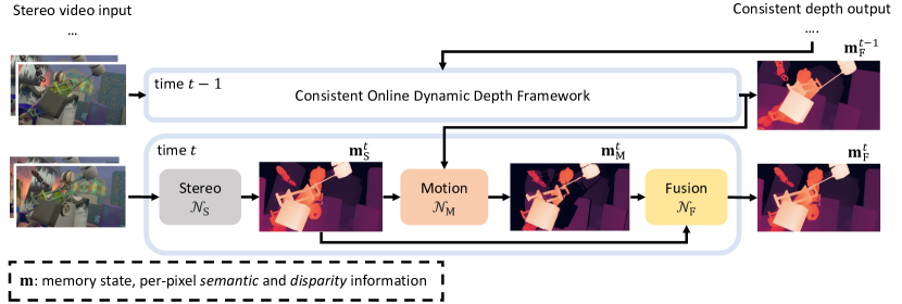
The goal of CODD is to estimate temporally consistent depth in dynamic scenes in an online setting. A stereo video stream is taken as input, where each image is of dimension . Let a memory state be a combination of per-pixel -channel semantic and 1-channel disparity information. CODD, as shown in Fig. 2, consists of three sub-networks:
-
–
A stereo network (Sect. 3.1) estimates the initial disparity and semantic feature map on a per-frame basis. The semantic information is encoded as feature maps and RGB values.
-
–
A motion network (Sect. 3.2) accounts for motion across frames by aligning the previous predictions to the current frame. Such motion information is also added to the semantic information for better fusion.
-
–
A fusion network (Sect. 3.3) that fuses the disparity estimates across time to promote the temporal consistency in an online setting.
We introduce the high-level concepts of each sub-network in the following sections and detail the designs in Appx A.
3.1 Stereo Network
The objective of the stereo network is to extract an initial estimate of disparity and semantic feature map on a per-frame basis. The stereo network takes the current stereo images as input and outputs the stereo memory state at time . Internally, it extracts semantic feature maps from the stereo images, and computes disparity by finding matches between the feature maps. In this paper, we use a recent network, HITNet [30], as our building block to estimate per-frame disparity due to its real-time speed and superior performance. In the subsequent sections, we discuss how to extend the stereo network to stabilize the disparity prediction temporally.
3.2 Motion Network
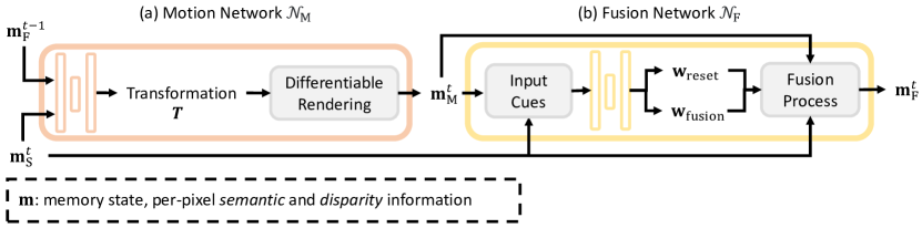
The motion network aligns the previous memory state with that of the current frame. Let denote the preceding memory state from our online consistent depth network at time . Our motion network , as shown in Fig. 3a, transforms into current frame based on :
where is the state from aligned to .
To perform such alignment, the inter-frame motion must be recovered. In a dynamic scene with camera movement and object movement/deformation, the motion prediction needs to be on a per-pixel level. Our motion network builds on top of RAFT3D [32] to predict a per-pixel SE3 transformation map . The motion is predicted using a GRU network and a Gauss-Newton optimization mechanism based on matching confidence for iterations. Once the motion between frames is recovered, we project the previous memory state to the current frame similar to [17] using differentiable rendering [28]:
| (1) |
where and are perspective and inverse perspective projection, respectively. Thus, the motion memory state resides in the current camera coordinate frame and has pixel-wise correspondence with the current prediction, which enables temporal aggregation of disparity. Additionally, we estimate a binary visibility mask by identifying the regions in the current frame that is not visible in the previous one. We also compute the confidence of motion via Sigmoid and compute the motion magnitude as the L2 norm of the scene flow. These information are added to the memory state for the fusion network to adaptively fuse the predictions. We detail differences between our motion network and RAFT3D and provide a quantitative comparison in Appx A.2.
3.3 Fusion Network
The objective of the fusion network (Fig. 3b) is to promote temporal consistency by aggregating the disparities of the motion and stereo memory states. The output of the fusion network is the fusion memory state :
| (2) |
where is the fusion network and contains the temporally consistent disparity estimate . We first discuss the fusion process (Sect. 3.3.1) and then cover the set of cues extracted from the memory states (Sect. 3.3.2) to guide such fusion process.
3.3.1 Fusion Process
The temporally consistent disparity is obtained by fusing the aligned and current disparity estimates. Let be the disparity from the motion network and be the disparity from the stereo network. The fusion network computes a reset weight and a fusion weight both of dimension . The fusion process of disparity estimates is formulated as:
| (3) |
The fusion memory state is thus formed by the fused disparity and semantic features extracted by the stereo network.
The intuition behind the fusion process is two-fold. First, it filters out outliers using . The outliers can be either induced by inaccurate disparity or motion predictions. In our work, is supervised to identify outliers whose errors are larger than the other disparity estimate by a threshold of . Second, the fusion process encourages temporal consistency by fusing current disparity prediction with reliable predictions propagated from the previous frame using . When disparity estimates are considered to be equally reliable within a threshold , the fusion network aggregates them with a regressed value between 0 and 1. As reset weights should already reject the most significant outliers, we set .
3.3.2 Input Cues
To determine the reset and fusion weights, we collect a set of input cues from and . We find explicit input cues are advantageous over the channel-wise concatenation of the two memory states.
First, the disparity confidence of and are computed. As disparities are computed mainly based on appearance similarity between the left and right images, we approximate the confidence of disparity prediction by computing the distance between the left and right features extracted from the stereo network. For robustness against matching ambiguity, we additionally offset each disparity estimate by and to collect local confidence information, forming a 3-channel confidence feature.
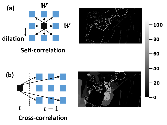
However, in the case of stereo occlusion, i.e. regions that are only visible in the left but not the right image, the disparity confidence based on appearance similarity becomes ill-posed. Thus, we additionally use the local smoothness information as a cue. We implement a pixel-to-patch self-correlation (Fig. 4a) to approximate the local smoothness information, which computes the correlation between a pixel and its neighboring pixels in a local patch of size , forming a correlation feature. Dilation may be used to increase the receptive field. We apply the pixel-to-patch self-correlation for both disparity and semantic features to acquire local disparity and appearance smoothness.
In the case of inaccurate motion predictions, the aligned memory state may contain wrong cross-frame correspondences. Therefore, the predictions in these regions need to be discarded as outliers. To promote such outlier rejection, the fusion network applies a pixel-to-patch cross-correlation (Fig. 4b) to evaluate the cross-frame disparity and appearance similarities. In cross-correlation, each pixel attends to a local patch of the previous image centered at the same pixel location after motion correction, forming a correlation feature. In our implementation, we use the distance for disparity and dot-products for appearance correlation.
Lastly, we observe that when the inter-frame motion is large, the motion estimate is less reliable and may thus result in wrong cross-frame correspondences. Therefore, we provide the flow magnitude and confidence as a motion cue. We additionally use the visibility mask from the projection process to identify the invalid regions and provide the semantic features for context information.
3.4 Supervision
Stereo and Motion Network We supervise the stereo network on the per-frame disparity estimate against the ground truth following [30]. We supervise the motion network on the transformation prediction T, with a loss imposed on its projected scene flow against the ground truth following [32].
Fusion Network We supervise the fusion network to promote temporal consistency of disparity estimates. We note that optimizing for disparity changes only may not be ideal, as errors in the previous frame will propagate to the current frame even if the predicted disparity change is correct. Therefore, we impose losses on the disparity prediction , and predicted weights .
We supervise the predicted disparity against the ground truth using Huber loss [10], denoted as the disparity loss .
Further, we supervise the reset weights such that they reject the worse prediction between the stereo and motion network disparity estimates. Let be the error of the motion disparity and be the error of the stereo disparity against the ground truth . Because rejects the motion disparity estimate when its value is zero (Eqn. 3), we impose a loss such that it favors zero when is worse and favors one when is better. Thus, we have
where is worse in condition 1) while is better in condition 2). Otherwise, the loss is zero as shown in condition 3).
The fusion weights are supervised such that they aggregate the past two disparity estimates correctly:
Different from the reset weights, the fusion weights are not only trained to identify the better estimate as shown in conditions 1) and 2), but also trained with an additional regularization term such that the fusion weights are around 0.5 when both estimates are considered equally good as shown in condition 3).
The final loss for fusion network training is computed as:
| (4) |
which is the weighted sum of and .
4 Experimental Setup
4.1 Implementation Details
We use a batch of 8 and Adam [14] as the optimizer on Nvidia V100 GPUs. Following [32], we use a linearly decayed learning rate of for pre-training and for fine-tuning. We pre-train motion and fusion networks for 25000 and 12500 steps, and halve the steps during fine-tuning. We perform steps of incremental updates in the motion network when datasets contain small motion (e.g. TartanAir [36]) and otherwise (e.g. FlyingThings3D [24], KITTI Depth [34] and KITTI 2015 [25]). In the fusion network, we use a patch size with dilation of 2 for pixel-to-patch correlation to increase the receptive field. By default, we set , , , and . Due to the sparsity of ground truth in KITTI datasets, supervising the fusion weights can be ill-posed as only a few pixels are aligned across time. We set .
4.2 Metrics
We propose to quantify the temporal inconsistency by a temporal end-point-error (TEPE) metric and the relative error () given cross-frame correspondences:
| (5) |
where are signed disparity change and avoids division by zero. Intuitively, TEPE and reflects the absolute and relative error between predicted and ground truth depth motion between two time points. TEPE is generally proportional to the ground truth magnitude and thus better reflects consistencies in pixels with large motion. better captures the consistencies of static pixels due to the weight. We also report threshold metrics of 3px for TEPE and 100% for (, ). Temporal metrics themselves can be limited as a network can be temporally consistent but wrong. Therefore, we also report the per-pixel disparity error using EPE and threshold metric of 3px (). We exclude pixels with extreme scene flow ( 210px) or disparity (1px or 210px) following [32] as they are generally outliers in our intended application. For all metrics, lower is better.
5 Results and Discussion
We first show quantitatively that current stereo depth estimation solutions suffer from poor temporal consistency (Sect. 5.1). We then show that CODD improves upon per-frame stereo networks and outperforms competing approaches across varied datasets, sharing the same stereo network without the need of re-training or fine-tuning (Sect. 5.2–Sect. 5.3). We lastly present ablation studies (Sect. 5.4) and inference time (Sect. 5.5) to characterize CODD.
5.1 Temporal Consistency Evaluation
We examine the temporal consistency of stereo depth techniques of different designs that operate on a per-frame basis. We use FlyingThings3D finalpass [24] dataset as it is commonly used for training stereo networks.
Results As shown in Tab. 1, all considered approaches have large TEPE and , with TEPE often larger than EPE and more than 14 times the ground truth disparity change as implied by . This suggests that the considered approaches suffer from poor temporal stability despite good per-pixel accuracy. A qualitative visualization is shown in Fig. 1. We show the resulting artifacts in the video supplement to further illustrate the case.
5.2 Pre-training on FlyingThings3D
We first demonstrate that CODD improves the temporal stability of per-frame networks by using the pre-trained HITNet [30] as our stereo network and freezing its parameters during training for a fair comparison. We follow the official split of FlyingThings3D. Tab. 2 summarizes the result.
Results To ensure temporal consistency, one naive way is to only forward the past information to the current frame. Thus, we compare the results of the per-frame prediction of the stereo network with the aligned preceding prediction of the motion network. To evaluate fairly, we fill occluded regions that are not observable in the past with . As shown in Tab. 2, the motion estimate is worse than stereo estimate due to outliers caused by wrong motion predictions as shown blue in Tab. 3, suggesting that only forwarding past information is not feasible. Nonetheless, performs on par with in most of the cases (white) and can even mitigate errors of that is hard to predict in the current frame (red). Thus, techniques to adaptively handle these cases can greatly reduce temporal noise.
While Kalman filter [13] successfully improves the temporal consistency by combining the two outputs, it leads to worse EPE. The result indicates that temporal consistency is indeed a different problem from per-frame accuracy. In contrast, CODD performs better in all metrics, which suggests that CODD achieves better stability across frames by pushing predictions toward the ground truth instead of propagating errors in time. We further show that our pipeline applies to other stereo networks in Appx C.1.
figureTemporal consistency comparison between stereo and motion predictions. While contains outliers (blue), it can also mitigate errors of (red). Our fusion network learns to adaptively fuse the estimates. Images from FlyingThings3D dataset [24].
![[Uncaptioned image]](/html/2111.09337/assets/x4.png)
| TEPE | EPE | ||||||
| TartanAir dataset [36] | Stereo [30] | 0.876 | 0.053 | 9.039 | 0.339 | 0.934 | 0.055 |
| Kalman Filter [13] | 0.829 | 0.053 | 7.501 | 0.252 | 0.935 | 0.055 | |
| CODD (Ours) | 0.751 | 0.045 | 6.206 | 0.240 | 0.904 | 0.053 | |
| KITTI Depth dataset [34] | Stereo [30] | 0.289 | 0.001 | 3.630 | 0.156 | 0.423 | 0.004 |
| Kalman Filter [13] | 0.278 | 0.001 | 2.615 | 0.125 | 0.431 | 0.005 | |
| CODD (Ours) | 0.258 | 0.001 | 2.764 | 0.132 | 0.418 | 0.003 | |
| KITTI 2015 dataset [25] | Stereo [30] | 0.570 | 0.026 | 10.672 | 0.126 | 0.811 | 0.033 |
| Kalman Filter [13] | 0.533 | 0.026 | 9.668 | 0.117 | |||
| CODD (Ours) | 0.507 | 0.022 | 8.740 | 0.112 | |||
5.3 Benchmark Results
We benchmark CODD across varied datasets. We first fine-tune the stereo network on each dataset to ensure good per-frame accuracy and keep it frozen for a fair comparison. We then fine-tune the motion and fusion networks, using the output of the stereo network as input. We summarize results in Tab. 3, provide end-to-end results in Appx C.2 and zero-shot results in Appx C.3.
Dataset TartanAir [36] is a synthetic dataset with simulated drone motions in different scenes. We use 15 scenes (219434 images) for training, 1 scene for validation (6607 images), and 1 scene (5915 images) for testing.
KITTI Depth [34] has footage of real-world driving scenes, where ground truth depth is acquired from LiDAR. We follow the official split and train CODD on 57 scenes (38331 images), validate on 1 scene (1100 images), and test on 13 scenes (3426 images). We use pseudo ground truth information inferred from an off-the-shelf optical flow network [31] trained on KITTI 2015.
KITTI 2015 [25] is a subset of KITTI Depth with 200 temporal image pairs. The data is complementary to KITTI Depth as ground truth optical flow information is provided, however, the long-term temporal consistency is not captured as there are only two frames for each scene. We train on 160 image pairs, validate on 20 image pairs, and test on 20 image pairs. Given the small dataset size, we perform five-fold cross-validation experiments and report the average results.
Results We find that CODD consistently outperforms the per-frame stereo network [30] across all metrics similar to findings in Sect. 5.2. The is improved by up to 31%, from 9.039 to 6.206 in the TartanAir dataset. Compared to the Kalman filter, CODD leads to smaller EPE in contrast to the Kalman filter, indicating both improved temporal and per-pixel performance. This again demonstrates the improved temporal performance does NOT guarantee improved per-pixel accuracy. We note that all settings in KITTI 2015 have the same EPE and , because we do not have ground truth information to evaluate the per-pixel accuracy of the fusion result of the second frame. More qualitative visualizations can be found in video supplement and Appx B.
5.4 Ablation Experiments
We conduct experiments on the FlyingThings3D dataset [24] to ablate the effectiveness of different sub-components.
5.4.1 Fusion Network
We summarize the key ablation experiments of the fusion network in Tab. 4 and provide additional results in Appx C.4.
| TEPE | EPE | ||||||
| a) Reset | 0.783 | 0.036 | 15.953 | 0.217 | 0.618 | 0.030 | |
| weight | ✓ | 0.756 | 0.035 | 15.013 | 0.211 | 0.604 | 0.029 |
| b) Fusion input cues | +FL | 0.763 | 0.035 | 15.103 | 0.211 | 0.604 | 0.029 |
| +V | 0.758 | 0.035 | 15.082 | 0.210 | 0.605 | 0.029 | |
| +SM | 0.756 | 0.035 | 15.013 | 0.211 | 0.604 | 0.029 | |
| c) Training | 2 | 0.756 | 0.035 | 15.013 | 0.211 | 0.604 | 0.029 |
| sequence | 3 | 0.753 | 0.035 | 14.942 | 0.211 | 0.600 | 0.029 |
| length | 4 | 0.741 | 0.034 | 15.205 | 0.214 | 0.595 | 0.028 |
a) Reset weights: In theory, only the fusion weight is needed between two estimates as it can reject outliers by estimating extreme values (e.g., 0 or 1). However, we find that predicting additional reset weights improves performance across all metrics. This may be attributed to the difference in supervision, where reset weights are trained for outlier detection, while fusion weights are trained for aggregation.
b) Fusion input cues: Other than the disparity confidence, self- and cross-correlation, we incrementally add the flow confidence/magnitude (+FL), visibility mask (+V), and semantic feature map (+SM) to the fusion networks. We find that the metrics improve marginally with additional inputs, especially for TEPE.
c) Training sequence length: During training, by default we train with sequences with a length of two frames, where the second frame takes the stereo outputs of the first frame as input. However, during the inference process, the preceding outputs are from the fusion network. Thus, to better approximate the inference process, we further extend the sequence length to three and four. We find that the fusion network consistently benefits from the increasing training sequence length. However, this elongates training time proportionally.
5.4.2 Empirical Best Case
We provide an empirical study of the “best case” of motion or fusion network in Tab. 5. For empirical best motion network , we use ground truth scene flow and set flow confidence to one. For empirical best fusion network , we pick the better disparity estimates pixel-wise between the stereo and motion estimates given ground truth disparity. We find that perfect motion leads to a substantial reduction in while perfect fusion leads to a substantial reduction in TEPE. In both cases, EPE also improves. While CODD performs well against competing approaches, advancing the motion or fusion networks has the potential to substantially improve temporal consistency.
| TEPE | EPE | |||||
| CODD (Ours) | 0.741 | 0.034 | 15.205 | 0.214 | 0.595 | 0.028 |
| Empirical best | 0.879 | 0.043 | 5.401 | 0.125 | 0.571 | 0.027 |
| Empirical best | 0.529 | 0.025 | 9.936 | 0.214 | 0.455 | 0.021 |
5.5 Inference Speed and Number of Parameters
The inference speed of CODD on images of resolution 640480 with is 25 FPS (stereo 26ms, motion 13ms, fusion 0.3ms) on an Nvidia Titan RTX GPU. The total number of parameters is 9.3M (stereo 0.6M, motion 8.5M, and fusion 0.2M). Compared to the stereo network, the overhead is mainly introduced by the motion network.
5.6 Limitations
While CODD outperforms competing methods across datasets, we recognize that there is still a gap between CODD and the empirical best cases in Sect. 5.4.2. Furthermore, CODD cannot correct errors when both current and previous frame estimates are wrong, as the weights between estimates in the fusion process are bounded to . Lastly, we design CODD to look at the immediately preceding frame only. Exploiting more past information may potentially lead to performance improvement.
6 Conclusions
We present a general framework to produce temporally consistent depth estimation for dynamic scenes in an online setting. CODD builds on contemporary per-frame stereo depth approaches and shows superior performance across different benchmarks, both in terms of temporal metrics and per-pixel accuracy. Future work may extend upon our motion or fusion network for better performance and extend to multiple past frames.
References
- [1] Alex M Andrew. Multiple view geometry in computer vision. Kybernetes, 2001.
- [2] Gualtiero Badin and Fulvio Crisciani. Variational formulation of fluid and geophysical fluid dynamics. Mech. Symmetries Conservation Laws, 2018.
- [3] D. J. Butler, J. Wulff, G. B. Stanley, and M. J. Black. A naturalistic open source movie for optical flow evaluation. In A. Fitzgibbon et al. (Eds.), editor, European Conf. on Computer Vision (ECCV), Part IV, LNCS 7577, pages 611–625. Springer-Verlag, Oct. 2012.
- [4] Jia-Ren Chang and Yong-Sheng Chen. Pyramid stereo matching network. In Proceedings of the IEEE Conference on Computer Vision and Pattern Recognition, pages 5410–5418, 2018.
- [5] MMSegmentation Contributors. MMSegmentation: Openmmlab semantic segmentation toolbox and benchmark. https://github.com/open-mmlab/mmsegmentation, 2020.
- [6] Chanho Eom, Hyunjong Park, and Bumsub Ham. Temporally consistent depth prediction with flow-guided memory units. IEEE Transactions on Intelligent Transportation Systems, 21(11):4626–4636, 2019.
- [7] Xiaoyang Guo, Kai Yang, Wukui Yang, Xiaogang Wang, and Hongsheng Li. Group-wise correlation stereo network. In Proceedings of the IEEE/CVF Conference on Computer Vision and Pattern Recognition, pages 3273–3282, 2019.
- [8] Kaiming He, Xiangyu Zhang, Shaoqing Ren, and Jian Sun. Deep residual learning for image recognition. In Proceedings of the IEEE conference on computer vision and pattern recognition, pages 770–778, 2016.
- [9] Heiko Hirschmuller. Stereo processing by semiglobal matching and mutual information. IEEE Transactions on pattern analysis and machine intelligence, 30(2):328–341, 2007.
- [10] Peter J Huber. Robust estimation of a location parameter. In Breakthroughs in statistics, pages 492–518. Springer, 1992.
- [11] Matthias Innmann, Michael Zollhöfer, Matthias Nießner, Christian Theobalt, and Marc Stamminger. Volumedeform: Real-time volumetric non-rigid reconstruction. ArXiv, abs/1603.08161, 2016.
- [12] Max Jaderberg, Karen Simonyan, Andrew Zisserman, et al. Spatial transformer networks. Advances in neural information processing systems, 28:2017–2025, 2015.
- [13] Rudolph Emil Kalman. A new approach to linear filtering and prediction problems. 1960.
- [14] Diederik P Kingma and Jimmy Ba. Adam: A method for stochastic optimization. arXiv preprint arXiv:1412.6980, 2014.
- [15] Johannes Kopf, Xuejian Rong, and Jia-Bin Huang. Robust consistent video depth estimation. In Proceedings of the IEEE/CVF Conference on Computer Vision and Pattern Recognition, pages 1611–1621, 2021.
- [16] Zhaoshuo Li, Xingtong Liu, Nathan Drenkow, Andy Ding, Francis X Creighton, Russell H Taylor, and Mathias Unberath. Revisiting stereo depth estimation from a sequence-to-sequence perspective with transformers. In Proceedings of the IEEE/CVF International Conference on Computer Vision, pages 6197–6206, 2021.
- [17] Zhaoshuo Li, Amirreza Shaban, Jean-Gabriel Simard, Dinesh Rabindran, Simon DiMaio, and Omid Mohareri. A robotic 3d perception system for operating room environment awareness. arXiv preprint arXiv:2003.09487, 2020.
- [18] Chao Liu, Jinwei Gu, Kihwan Kim, Srinivasa G Narasimhan, and Jan Kautz. Neural rgb (r) d sensing: Depth and uncertainty from a video camera. In Proceedings of the IEEE/CVF Conference on Computer Vision and Pattern Recognition, pages 10986–10995, 2019.
- [19] Xiaoxiao Long, Lingjie Liu, Wei Li, Christian Theobalt, and Wenping Wang. Multi-view depth estimation using epipolar spatio-temporal networks. In Proceedings of the IEEE/CVF Conference on Computer Vision and Pattern Recognition, pages 8258–8267, 2021.
- [20] Yonghao Long, Zhaoshuo Li, Chi Hang Yee, Chi Fai Ng, Russell H Taylor, Mathias Unberath, and Qi Dou. E-dssr: Efficient dynamic surgical scene reconstruction with transformer-based stereoscopic depth perception. In International Conference on Medical Image Computing and Computer-Assisted Intervention, pages 415–425. Springer, 2021.
- [21] Xuan Luo, Jia-Bin Huang, Richard Szeliski, Kevin Matzen, and Johannes Kopf. Consistent video depth estimation. ACM Transactions on Graphics (TOG), 39(4):71–1, 2020.
- [22] Wei-Chiu Ma, Shenlong Wang, Rui Hu, Yuwen Xiong, and Raquel Urtasun. Deep rigid instance scene flow. In Proceedings of the IEEE/CVF Conference on Computer Vision and Pattern Recognition, pages 3614–3622, 2019.
- [23] Sergey Matyunin, Dmitriy Vatolin, Yury Berdnikov, and Maxim Smirnov. Temporal filtering for depth maps generated by kinect depth camera. In 2011 3DTV Conference: The True Vision-Capture, Transmission and Display of 3D Video (3DTV-CON), pages 1–4. IEEE, 2011.
- [24] Nikolaus Mayer, Eddy Ilg, Philip Hausser, Philipp Fischer, Daniel Cremers, Alexey Dosovitskiy, and Thomas Brox. A large dataset to train convolutional networks for disparity, optical flow, and scene flow estimation. In Proceedings of the IEEE conference on computer vision and pattern recognition, pages 4040–4048, 2016.
- [25] Moritz Menze, Christian Heipke, and Andreas Geiger. Joint 3d estimation of vehicles and scene flow. ISPRS annals of the photogrammetry, remote sensing and spatial information sciences, 2:427, 2015.
- [26] Richard A Newcombe, Dieter Fox, and Steven M Seitz. Dynamicfusion: Reconstruction and tracking of non-rigid scenes in real-time. In Proceedings of the IEEE conference on computer vision and pattern recognition, pages 343–352, 2015.
- [27] Adam Paszke, Sam Gross, Francisco Massa, Adam Lerer, James Bradbury, Gregory Chanan, Trevor Killeen, Zeming Lin, Natalia Gimelshein, Luca Antiga, et al. Pytorch: An imperative style, high-performance deep learning library. Advances in neural information processing systems, 32:8026–8037, 2019.
- [28] Nikhila Ravi, Jeremy Reizenstein, David Novotny, Taylor Gordon, Wan-Yen Lo, Justin Johnson, and Georgia Gkioxari. Accelerating 3d deep learning with pytorch3d. arXiv:2007.08501, 2020.
- [29] Denis Tananaev, Huizhong Zhou, Benjamin Ummenhofer, and Thomas Brox. Temporally consistent depth estimation in videos with recurrent architectures. In Proceedings of the European Conference on Computer Vision (ECCV) Workshops, pages 0–0, 2018.
- [30] Vladimir Tankovich, Christian Hane, Yinda Zhang, Adarsh Kowdle, Sean Fanello, and Sofien Bouaziz. Hitnet: Hierarchical iterative tile refinement network for real-time stereo matching. In Proceedings of the IEEE/CVF Conference on Computer Vision and Pattern Recognition, pages 14362–14372, 2021.
- [31] Zachary Teed and Jia Deng. Raft: Recurrent all-pairs field transforms for optical flow. In European conference on computer vision, pages 402–419. Springer, 2020.
- [32] Zachary Teed and Jia Deng. Raft-3d: Scene flow using rigid-motion embeddings. In Proceedings of the IEEE/CVF Conference on Computer Vision and Pattern Recognition, pages 8375–8384, 2021.
- [33] Iraklis Tsekourakis and Philippos Mordohai. Measuring the effects of temporal coherence in depth estimation for dynamic scenes. In Proceedings of the IEEE/CVF Conference on Computer Vision and Pattern Recognition Workshops, pages 0–0, 2019.
- [34] Jonas Uhrig, Nick Schneider, Lukas Schneider, Uwe Franke, Thomas Brox, and Andreas Geiger. Sparsity invariant cnns. In 2017 international conference on 3D Vision (3DV), pages 11–20. IEEE, 2017.
- [35] Jingdong Wang, Ke Sun, Tianheng Cheng, Borui Jiang, Chaorui Deng, Yang Zhao, Dong Liu, Yadong Mu, Mingkui Tan, Xinggang Wang, et al. Deep high-resolution representation learning for visual recognition. IEEE transactions on pattern analysis and machine intelligence, 2020.
- [36] Wenshan Wang, Delong Zhu, Xiangwei Wang, Yaoyu Hu, Yuheng Qiu, Chen Wang, Yafei Hu, Ashish Kapoor, and Sebastian Scherer. Tartanair: A dataset to push the limits of visual slam. In 2020 IEEE/RSJ International Conference on Intelligent Robots and Systems (IROS), pages 4909–4916. IEEE, 2020.
- [37] Greg Welch, Gary Bishop, et al. An introduction to the kalman filter. 1995.
- [38] Gengshan Yang and Deva Ramanan. Upgrading optical flow to 3d scene flow through optical expansion. In Proceedings of the IEEE/CVF Conference on Computer Vision and Pattern Recognition, pages 1334–1343, 2020.
- [39] Tao Yu, Kaiwen Guo, Feng Xu, Yuan Dong, Zhaoqi Su, Jianhui Zhao, Jianguo Li, Qionghai Dai, and Yebin Liu. Bodyfusion: Real-time capture of human motion and surface geometry using a single depth camera. 2017 IEEE International Conference on Computer Vision (ICCV), pages 910–919, 2017.
- [40] Haokui Zhang, Chunhua Shen, Ying Li, Yuanzhouhan Cao, Yu Liu, and Youliang Yan. Exploiting temporal consistency for real-time video depth estimation. In Proceedings of the IEEE/CVF International Conference on Computer Vision, pages 1725–1734, 2019.
- [41] Zhoutong Zhang, Forrester Cole, Richard Tucker, William T Freeman, and Tali Dekel. Consistent depth of moving objects in video. ACM Transactions on Graphics (TOG), 40(4):1–12, 2021.
Acknowledgements We thank Johannes Kopf and Michael Zollhoefer for helpful discussions, and Vladimir Tankovich for HITNet implementation. We thank anonymous reviewers and meta-reviewers for their feedback on the paper. This work was done during an internship at Reality Labs, Meta Inc and funded in part by NIDCD K08 Grant DC019708.
Appendix A Network Details
Our code base is built upon MMSegmentation [5].
A.1 Stereo Network
We use HITNet [30] as our per-frame stereo network to extract disparity and features on a per-frame basis. HITNet builds an initial cost volume with a pre-specified disparity range. In our implementation, we set the maximum disparity to be 320 following the original implementation. The channel size of extracted features is 24, which is used in the fusion network to evaluate disparity confidence. The memory state generated by the stereo network includes the frame-wise estimated disparity, the feature of left and right images at the 1/4 resolution for disparity confidence computation, and the left RGB image.
Our HITNet code is adapted from open-sourced implementation111https://github.com/MJITG/PyTorch-HITNet-Hierarchical-Iterative-Tile-Refinement-Network-for-Real-time-Stereo-Matching222https://github.com/meteorshowers/X-StereoLab in PyTorch [27] and confirmed by the authors of HITNet. We note that the HITNet adapted is based on Table 6 of [30] instead of the HITNet XL or HITNet L in Table 1 of [30]. As HITNet works across different datasets (Table 2-4 in [30]), we have chosen HITNet as our stereo network. As described in Sect.4.2, we remove pixels with extreme scene flow (210px) and disparity (1px or 210px). These removed pixels correspond to unrealistically fast, far, or close objects during simulation, which are not considered in our intended applications such as augmented reality. In comparison, [30] removes pixels with disparity 192px. Thus, the reported per-pixel accuracy performance differs slightly on FlyingThings3D.
A.2 Motion Network
Our motion network builds on top of RAFT3D [32]. Specifically, we adapt the inter-frame transformation T estimation process. We first provide the necessary background of the estimation process and detail the difference between our motion network and RAFT3D next paragraph. Let be a location in pixel coordinates and be a location in Cartesian coordinates. RAFT3D uses a context extractor to provide semantic information for object grouping, and a feature extractor for cross-frame correspondence matching. A piece-wise rigid constraint is realized by grouping pixels based on their motion and appearance similarities and enforcing the motion within a group to be the same. The GRU module takes the image context feature, correlation information, estimated transformation, and corresponding scene flow as input. The GRU then makes corrections to the scene flow, extracts a set of rigid-embeddings , and associated confidence of estimates . A differentiable Gauss-Newton (GN) optimization step is performed to update the transformation based on the residual error (Eq. 6). The update scheme is iterative for steps, with the transformation and flow initialized to identity and zero respectively. Given the i-th pixel at and its local neighborhood pixels , the k-th iteration residual error to be minimized is:
| (6) | ||||
| (7) | ||||
| (8) |
where is the incremental motion on the SE3 manifold to be made to the previous transformation , is the raw predicted scene flow, is weighted norm, is the flow confidence, and is the distance of rigid-embeddings. The updated transformation is . The final scene flow-induced transformation from transformation prediction T in image coordinate can be computed as:
| (9) |
The magnitude and confidence of the flow is used later in fusion network.
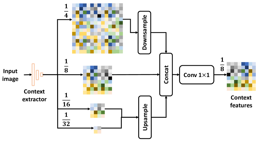
The difference between the transformation T prediction process of our motion network and RAFT3D is summarized in this paragraph. As shown in Eq. 6, the similarities between rigid embeddings of pixels critically determine if two pixels are grouped as the same object. Thus, generating high-quality rigid embeddings has a direct impact on motion accuracy. Originally, RAFT3D uses a pre-trained ResNet-50 [8] as the context extractor to provide semantics information. Instead, we replace the pre-trained ResNet-50 with a network similar to HRNet [35] that aggregates the context information across hierarchical levels. An overview is shown in Fig. 5. The context extractor extracts the semantic information from four resolutions – , and resolutions. We use bilinear upsampling to resize all feature maps to the resolution and use one convolution to aggregate the information. Compared to ResNet-50, which has 40M parameters, our context extractor only has 3M parameters. We found that our motion network outperforms RAFT3D on the FlyingThings3D [24] dataset while having 1/5-th of the parameters of RAFT3D. In our implementation, we use the RGB image as semantic input instead of features from stereo to reduce dependency on the stereo network.
Once inter-frame motion T is recovered, we use differentiable rendering [28] to forward-project all feature maps [17] from the previous frame to the current frame, which is equivalent to Lagrangian flow where pixels of the past frame are pushed to the current frame. This is in contrast to Eularian flow, where pixels are pulled [2], which is proposed in Spatial Transformer [12] and implemented as the “grid_sample” function in PyTorch [27].
We evaluate the accuracy of the transformation map T of our motion network because accurate motion prediction is critical to our process. We compare the performance of our motion network and RAFT3D in Tab. 6. To quantify the accuracy of T, we report the flow EPE (FEPE) on optical flow and scene flow , and threshold metrics of 1px following [32]. We evaluate the performance in two settings, 1) taking the ground truth disparity as input and 2) taking the noisy stereo disparity estimates as input. For a fair comparison, we re-train RAFT3D using our training setup and report its result. CODD performs better than RAFT3D in both and regardless of the input type, with only 1/5-th of the parameters of RAFT3D.
A.3 Fusion Network
The fusion network uses a set of input cues to determine the and . For appearance correlation, we project the input features from the stereo network to a feature dimension of 32. The fusion weight is then regressed at resolution for better context awareness while the reset weight is regressed at the full resolution for better outlier rejection.
| TEPE | EPE | |||||
| STTR | 0.482 | 0.014 | 11.434 | 0.374 | 0.449 | 0.014 |
| STTR + CODD | 0.448 | 0.017 | 10.109 | 0.290 | 0.454 | 0.014 |
| PSMNet | 1.371 | 0.056 | 35.136 | 0.466 | 1.079 | 0.045 |
| PSMNet + CODD | 1.266 | 0.052 | 31.958 | 0.354 | 1.052 | 0.044 |
| GwcNet | 0.959 | 0.041 | 22.598 | 0.409 | 0.752 | 0.032 |
| GwcNet + CODD | 0.924 | 0.039 | 19.953 | 0.402 | 0.726 | 0.032 |
Appendix B Qualitative Visualization
B.1 Space-time volume
Similar to [41], we visualize the network’s output by concatenating the predictions over the temporal axis to build a space-time volume on the MPI Sintel dataset. We then take a slice along the horizontal axis and visualize the depth prediction over time in Fig. 6. Even though this does not trace the same object point over time, it gives insights into how stable the model’s prediction is temporally. We find that CODD contains less high-frequency variation than the per-frame model.
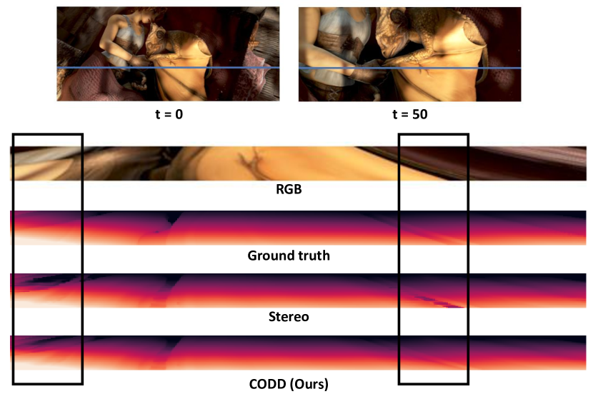
© copyright Blender Foundation durian.blender.org
B.2 Improvements over Per-frame Stereo
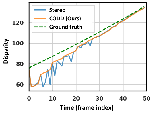
We visualize the improvements over stereo qualitatively in Fig. 7. As ground truth disparity constantly increases, the stereo predictions vary frequently. By incorporating temporal information, CODD removes many of the temporal jitters of the stereo prediction and outputs more consistent and accurate estimates.
We plot the distribution of TEPE comparing our and stereo’s results in Fig. 8. We find that CODD successfully reduce TEPE across different magnitudes as shown in Fig. 8a, suggesting more consistent predictions across time. To understand how the performance of each pixel has changed instead of the whole image, we additionally plot the TEPE of each pixel of the stereo network and CODD in Fig. 8b with one-to-one correspondence, where the diagonal line indicates break-even (i.e., TEPE of both networks are the same), top left region indicates that CODD successfully reduces the TEPE, and bottom right region indicates that CODD makes the TEPE larger. As most of the plotted points are clustered in the top left region, i.e., our TEPE is smaller than stereo network TEPE, CODD reduces TEPE of the stereo network for the majority of the pixels. We note that even in the cases where the TEPE of the stereo network is large (y-axis), CODD can reduce the error close to zero (x-axis), suggesting large improvements in terms of temporal consistency over the stereo network for these cases.

Appendix C Additional Experiments
We include additional experiments that shed light on CODD in the following sections.
C.1 Using Different Stereo Networks
We present additional experiments on FlyingThings3D [24] to demonstrate that our framework works with different stereo networks. We follow the same experimental setup as Sect.5.2 and use other stereo networks to produce the per-frame disparity estimates. Tab. 7 summarizes our findings, which are consistent with our findings for HITNet. We note that all metrics improve with the introduction of our motion and fusion networks, with the only exceptions of STTR , EPE and GwcNet . The results suggest that our proposed framework should apply to other stereo networks.
C.2 End-to-End Fine-tuning
We note that our framework is designed to be end-to-end differentiable. Thus, during fine-tuning, we can in theory directly fine-tune all components together, instead of first fine-tuning the stereo network and then the other components. However, due to the gradients from different losses back-propagating to the stereo network, in comparison to only the stereo losses in the case of a per-frame stereo network, end-to-end fine-tuning may not be a fair comparison. Thus, we report these additional results in the appendix.
Denoting the loss of stereo network as , the loss of motion network as , and the loss of fusion network as , during end-to-end fine-tuning, the total loss is the weighted sum of all sub-network losses:
| (10) |
We use while keeping in our experiments to balance the losses. A batch size of 16 is used for end-to-end fine-tuning due to memory constraints. All learning rates are linearly decayed from following the learning rate of the per-frame stereo model.
The results on different benchmarks are summarized in Tab. 8, where the end-to-end training (E2E) result is comparable to the stage-wise fine-tuning results in Sect.5.3. Other than TartanAir, end-to-end fine-tuning leads to better results. In either training setup, our results are favorable compared to the per-frame results. The results suggest that our framework is not sensitive to the specific training strategies we have used.
| TEPE | EPE | ||||||
| Tartan Air dataset [36] | Stereo [30] | 0.876 | 0.053 | 9.039 | 0.339 | 0.934 | 0.055 |
| CODD | 0.751 | 0.045 | 6.206 | 0.240 | 0.904 | 0.053 | |
| CODD (E2E) | 0.763 | 0.047 | 6.976 | 0.270 | 0.905 | 0.052 | |
| KITTI Depth dataset [34] | Stereo [30] | 0.289 | 0.001 | 3.630 | 0.156 | 0.423 | 0.004 |
| CODD | 0.258 | 0.001 | 2.764 | 0.132 | 0.418 | 0.003 | |
| CODD (E2E) | 0.251 | 0.001 | 2.408 | 0.129 | 0.409 | 0.003 | |
| KITTI 2015 dataset [25] | Stereo [30] | 0.570 | 0.026 | 10.672 | 0.126 | 0.811 | 0.033 |
| CODD | 0.507 | 0.022 | 8.740 | 0.112 | |||
| CODD (E2E) | 0.505 | 0.024 | 8.132 | 0.111 | 0.806 | 0.032 | |
C.3 Zero-shot Generalization
Dataset We report zero-shot generalization results of our pre-trained network from FlyingThings3D on the TartanAir, KITTI Depth, and MPI Sintel dataset finalpass [3]. MPI Sintel contains animated characters with deformation. It contains 23 video sequences, totaling 1064 images.
C.4 Additional Fusion Network Ablation
We provide additional ablation experiments to further understand how different design choices may affect the performance in Tab. 10.
Correlation window We experiment with different correlation window size to see the effect of increasing receptive field. We increase the correlation window size of correlation from 3 to 5 or 7, with a constant dilation of 2. We do not observe significant benefits of increasing the window size. The result suggests that a window size of 3 with dilation of 2 already provides enough information for the network. Our final model uses a window size of 3 for efficiency.
Correlation type In addition to our proposed pixel-to-patch correlation, we also experiment with: 1) pixel-to-pixel correlation, where correlation values are obtained pixel-wise, and 2) patch-to-patch correlation, where correlation values are computed pixel-wise over the whole patch. We find that pixel-to-patch correlation performs best across all metrics.
| TEPE | EPE | ||||||
| Correlation | 3 | 0.756 | 0.035 | 15.013 | 0.211 | 0.604 | 0.029 |
| window | 5 | 0.756 | 0.035 | 15.005 | 0.210 | 0.603 | 0.029 |
| 7 | 0.756 | 0.035 | 15.014 | 0.210 | 0.603 | 0.029 | |
| Correlation Type | pixel-to-patch | 0.756 | 0.035 | 15.013 | 0.212 | 0.604 | 0.029 |
| pixel-to-pixel | 0.758 | 0.036 | 15.103 | 0.211 | 0.610 | 0.030 | |
| patch-to-patch | 0.759 | 0.035 | 15.134 | 0.210 | 0.609 | 0.030 | |
Appendix D Dataset Details
For long sequences (several thousand), we chunk the video into sub-sequences of 50 frames following [3].
FlyingThings3D: We follow the official split information.
TartanAir: We validate on the seasonforest sequence and test on the carwelding sequence.
KITTI Depth [34]333http://www.cvlibs.net/datasets/kitti/eval_depth_all.php: We follow the official split on the KITTI Depth dataset, except the People scene for training due to little variation. We use the last training sequence 2011_10_03_drive_0042_sync for validation. Due to the missing ground truth optical flow information, we use an off-the-shelf network to generate the optical flow information [31] and use forward-backward flow consistency to determine flow occluded regions and outliers. The disparity change is then computed from optical flow.
KITTI 2015 [25]444http://www.cvlibs.net/datasets/kitti/eval_scene_flow.php: We use a 5-fold split that splits the data into train, validation, test data.
Appendix E Training Stereo Depth Network in Multi-frame Setting
One of the simplest ideas we have tried to improve the temporal consistency of stereo depth networks is to train stereo networks in a multi-frame setting instead of randomly sampling images from the whole dataset. For a fair comparison, we reduce the cropping height by two times and insert a subsequent frame from the same video sequence, such that the total number of pixels that the network sees is the same. However, we find this does not perform well compared to the original training scheme as shown in Tab. 11, which may be attributed to the reduced diversity in the sample size.
| TEPE | TEPE | EPE | |
| default training | 0.821 | 16.450 | 0.609 |
| multi-frame training | 0.998 | 19.199 | 0.715 |
Appendix F Optical Flow as Alignment Mechanism
One alternative to our motion network is to predict an inter-frame optical flow (i.e. without disparity change compared to scene flow) to provide past information. However, since depth is not translation invariant, the past information can only provide past trending information instead of being directly aggregated. As a proof-of-concept, we replace the motion network with the ground truth optical flow provided to test the optical flow idea. However, we find that the temporal stability often doesn’t benefit from the past information, and in fact, becomes worse on the FlyingThings3D dataset.