Optimization of Grant-Free NOMA with Multiple Configured-Grants for mURLLC

Abstract

Massive Ultra-Reliable and Low-Latency Communications (mURLLC), which integrates URLLC with massive access, is emerging as a new and important service class in the next generation (6G) for time-sensitive traffics and has recently received tremendous research attention. However, realizing efficient, delay-bounded, and reliable communications for a massive number of user equipments (UEs) in mURLLC, is extremely challenging as it needs to simultaneously take into account the latency, reliability, and massive access requirements. To support these requirements, the third generation partnership project (3GPP) has introduced enhanced grant-free (GF) transmission in the uplink (UL), with multiple active configured-grants (CGs) for URLLC UEs. With multiple CGs (MCG) for UL, UE can choose any of these grants as soon as the data arrives. In addition, non-orthogonal multiple access (NOMA) has been proposed to synergize with GF transmission to mitigate the serious transmission delay and network congestion problems. In this paper, we develop a novel learning framework for MCG-GF-NOMA systems with bursty traffic. We first design the MCG-GF-NOMA model by characterizing each CG using the parameters: the number of contention-transmission units (CTUs), the starting slot of each CG within a subframe, and the number of repetitions of each CG. Based on the model, the latency and reliability performances are characterized. We then formulate the MCG-GF-NOMA resources configuration problem taking into account three constraints. Finally, we propose a Cooperative Multi-Agent based Double Deep Q-Network (CMA-DDQN) algorithm to balance the allocations of the channel resources among MCGs so as to maximize the number of successful transmissions under the latency constraint. Our results show that the MCG-GF-NOMA framework can simultaneously improve the low latency and high reliability performances in massive URLLC.

I Introduction

In the standardization of the Fifth Generation (5G) New Radio (NR), three communication service categories were defined to address the requirements of novel Internet of Things (IoT) use cases [1]. Among them, the Ultra-Reliable and Low-Latency Communications (URLLC) is one of the most challenging services with stringent low latency and high reliability requirements, i.e., in the Third Generation Partnership Project (3GPP) standard [2], a general URLLC requirement is $1-10^{-5}$ target reliability within 1 ms user plane latency. Considering the explosive increase in the number of IoT devices, it is essential to improve the access performance in networks for accommodating massive access with various requirements. Integrating URLLC with massive access, massive URLLC (mURLLC) wireless networks are able to realize efficient, delay-bounded, and reliable communications for a massive number of IoT devices[3]. The mURLLC is becoming a new and important service class in the next generation (6G) for the time-sensitive traffics and has received tremendous research attention[4]. However, addressing the need in mURLLC is fundamentally challenging as it needs to simultaneously guarantee the latency, reliability, and massive access requirements.

To support these requirements, several new features such as configured-grant (CG) transmission with automatic repetitions[5], user-equipment (UE) multiplexing[6], and multiple active CGs for URLLC UEs[7] were standardized by the 3GPP.

I-1 Grant-Free NOMA

To reduce the latency in URLLC, the grant-free (GF) (a.k.a. configured-grant (CG)) transmission is proposed for 5G NR in 3GPP Release 15[5] as an alternative for traditional grant-based (GB) (a.k.a. dynamic-grant (DG)) in Long Term Evolution (LTE). In NR GF transmission, the UE is allowed to transmit data to the Base Station (BS) in an arrive-and-go manner without scheduling request (SR) and uplink (UL) resource grant (RG) to reduce latency. To increase the reliability in URLLC, the K-repetition GF transmission has been proposed by 3GPP, where a pre-defined number of consecutive replicas of the same packet are transmitted in the consecutive time slots[5]. More details about K-repetition GF transmission can be found in [8]. To mitigate the serious transmission delay and network congestion problems caused by collision events in contention-based GF transmission and enhance the uplink connectivity, non-orthogonal multiple access (NOMA) has been proposed to synergize with GF transmission [6, 9], where GF-NOMA allows multiple UEs to transmit over the same physical resource by employing user-specific signature patterns (e.g, codebook, pilot sequence, mapping pattern, demodulation reference signal, power, etc.)[10].

I-2 Multiple Configured-Grants for Grant-Free NOMA

3GPP proposed multiple CGs (MCG) transmission in Release 16 [7] to support different starting offsets of the resources with respect to UL packet arrival time as shown in Fig. 1.

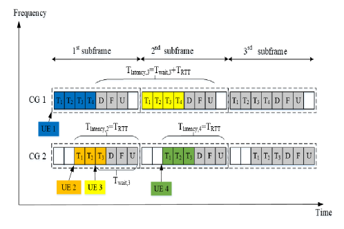
Figure 1: Multiple CGs (MCG) configurations for K-repetition GF transmission, T: packet transmission, D: DL processing, F: ACK/NACK feedback, and U: UL processing.

On the one hand, there is a chance of reducing the latency in cases where the data of an UE arrives (i.e., UE is active) after the starting slot offset of the CG 1 (UE 2, 3, and 4 in Fig. 1). As illustrated in Fig. 1, UE 2 can transmit using the CG 2 without waiting for the CG period in the next subframe as in the single CG (SCG). On the other hand, there is a chance of mitigating the collision events when multiple UEs are active and waiting for the CG period to transmit the packet. For example, UE 2 and UE 3 can transmit using different CG resources without collision as shown in Fig. 1. Multiple CGs also support different resource sizes, repetitions, and periodicity, to suit different data requirements, respectively[11, 12].

I-A Related Works

Scanning the open literature, to the best of our knowledge, most works focused on the analysis or optimization of single configured-grant GF-NOMA (SCG-GF-NOMA) transmissions.

In terms of analysis, a GF-NOMA strategy was proposed in [13], in which active devices transmitted data over a randomly selected available channel. In order to allow the receiver decode successfully, the transmitted data was encoded with rateless code. In [14], a new GF-NOMA analytical framework was proposed and the expressions for outage probability and throughput for GF-NOMA transmissions were derived, by treating collisions as interference through successive joint decoding or successive interference cancellation (SIC). In [15], a semi-GF scheme has been proposed, where the dedicated GB access was provided for one user while GF access was used by other users.

In terms of optimization, several studies have applied deep reinforcement learning (DRL) to optimize the SCG-GF-NOMA networks. DRL can obtain better resource allocation with near-optimal resource access probability distribution to improve the SCG-GF-NOMA transmission[16]. In [16], the authors designed users and sub-channel clusters in a region to reduce collisions of the GF-NOMA system. The formulated long-term cluster throughput problem is solved via DRL algorithm for optimal sub-channel and power allocation. In [17], the authors introduced power-domain NOMA to further improve network throughput and defined a new reward that enabled only one acknowledgement bit returning to the device from the BS in each time slot. In [18], the authors proposed two distributed Q-learning aided uplink GF-NOMA schemes to maximize the number of accessible devices, where the bursty traffic of massive Machine Type Communications (mMTC) devices is carefully considered.

Different from [13, 14, 15, 16, 17, 18], we aim to first design a novel framework about multiple CGs GF-NOMA (MCG-GF-NOMA) networks and optimize the long-term successfully served UEs under the latency constraint based on this framework for mURLLC service.

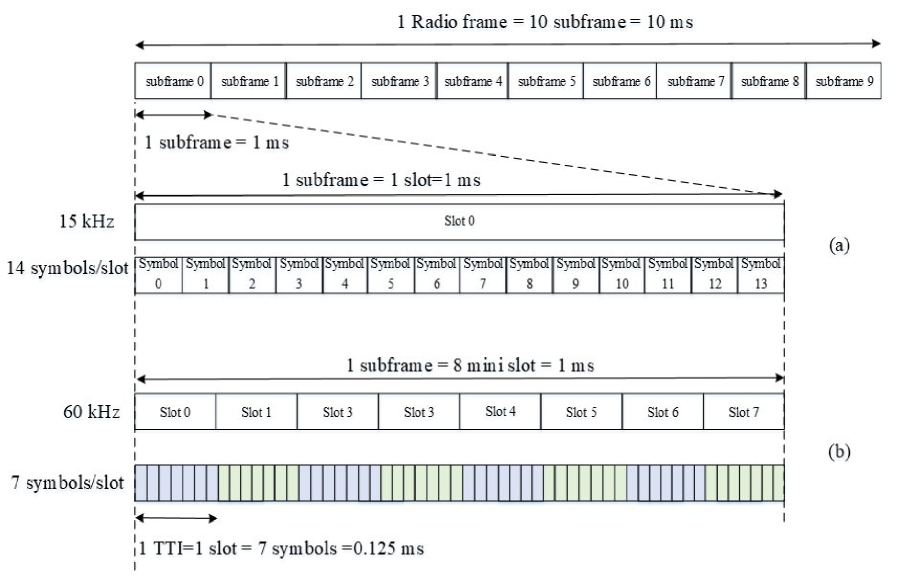
Figure 2: 5G NR frame structure for numerology: (a) 15 kHz with 14 symbols/slot, (b) 60 kHz with 7 symbols/mini-slot.

I-B Motivations and Contributions

As mentioned before, research on the MCG-GF-NOMA networks to support mURLLC is fundamental and essential, which is an untreated and challenging problem. To cope with it, accurately modeling, analyzing, and optimizing the MCG-GF-NOMA resource is fundamentally important, but the interplay between latency and reliability brings extra complexity. In addition, in the GF-NOMA scheme, the data is transmitted along with the pilot randomly, which is unknown at the BS and can lead to new research problems. The blind detection of active UEs is needed due to that the set of active users is unknown to the BS, which also brings extra challenges. The MCG-GF-NOMA system optimization can hardly be solved via the traditional convex optimization method, due to the complex communication environment with the lack of tractable mathematical formulations, whereas Reinforcement Learning (RL), can be a potential alternative approach, due to that it solely relies on the self-learning of the environment interaction, without the need to derive explicit optimization solutions based on a complex mathematical model. In this paper, we address the following fundamental questions: 1) how to design the MCG-GF-NOMA network; 2) how to quantify the URLLC reliability and latency performances in the MCG-GF-NOMA network; 3) how to formulate the MCG-GF-NOMA resources configuration problem taking into account the reliability and latency; and 4) how to balance the allocations of channel resources among multiple CGs so as to provide maximum success transmissions in mURLLC scenario with bursty traffic. The main contributions of this paper are as follows:

• We propose a novel MCG-GF-NOMA learning framework for attaining the long-term successfully served UEs under the latency constraint in mURLLC service, where the latency and reliability performances are characterized and analyzed for each CG. In this framework, we practically simulate the random traffics, the resource configuration, the collision detection, and the data decoding procedures.

• We design a MCG-GF-NOMA system, where we characterize each CG using the parameters including the number of contention-transmission units (CTUs), the starting slot of each CG within a subframe, and the number of repetitions of each CG. We then formulate the MCG-GF-NOMA resource configuration problem taking into account three constraints: 1) the CTU resource constraint is set to compare the MCG-GF-NOMA scheme with the SCG-GF-NOMA scheme; 2) the latency constraint is set to satisfy the latency requirement; and 3) the starting slot constraint is set to support various UL packet arrival times.

• We propose a Cooperative Multi-Agent learning technique based Double Deep Q-Network (CMA-DDQN) algorithm to balance the allocations of resources among MCGs so as to maximize the number of successful transmissions under the latency constraint, which breaks down the selection of high-dimensional parameters into multiple parallel sub-tasks with a number of DDQN agents cooperatively being trained to produce each parameter.

• Our results show that the MCG-GF-NOMA learning framework can improve the low latency and high realibity performances in a massive URLLC scenario. First, the number of successfully served UEs in the MCG-GF-NOMA system is up to four times more than that in the SCG-GF-NOMA system, and the latency of successfully served UEs in the MCG-GF-NOMA system is circa half of that in the SCG-GF-NOMA system. Second, the MCG-GF-NOMA learning framework can also increase the CTU resource utilization efficiency compared to the SCG-GF-NOMA system.

I-C Organization

The remainder of this paper is structured as follows. Section II illustrates the system model of MCG-GF-NOMA system. Section III describes the problem analysis and formulation. Section IV elaborates on the proposed CMA-DDQN algorithm for solving the formulated problem. The simulation results are illustrated in Section V. Finally, Section VI concludes the main concept, insights and results of this paper.

II System Model

We consider a single-cell uplink wireless network with a coverage radius of $R$. Particularly, a BS is located at the center of the cell, and a number of $N_{\rm UE}$ static UEs are randomly distributed around the BS in an area of the plane $\mathbb{R}^{2}$, where the UEs remain spatially static once deployed. The BS is unaware of the status of these UEs, hence no uplink channel resource is scheduled to them in advance. To capture the effects of the physical radio, we consider the standard power-law path-loss model with the path-loss attenuation $r^{-\eta}$, where $r$ is the Euclidean distance between the UE and the BS and $\eta$ is the path-loss attenuation factor. In addition, we consider a Rayleigh flat-fading environment, where the channel power gains $h$ are exponentially distributed (i.i.d.) random variables with unit mean.

II-A 5G NR Frame Structure and Numerologies

5G NR defines five numerologies based on subcarrier spacing (SCS) $\Delta f={2^{\mu}}\times 15$ kHz, where $\mu=0,1,2,3,4$ is the numerology factor [19], instead of a single value of 15 kHz in LTE. This feature reduces transmission time by decreasing the slot length as shown in Fig. 2. As depicted in Fig. 2, the per frame duration in NR is still 10 ms, and the same as in LTE. One frame consists of 10 subframes and each with 1 ms duration. With the increased SCS, i.e., a large value of $\mu$, the slot duration reduces according to $1/2^{\mu}$ ms. To further reduce the latency by shortening transmission time interval (TTI), in 5G NR, a TTI can be a mini-slot of 2, 4, or 7 Orthogonal Frequency Division Multiplexing (OFDM) symbols instead of 14 OFDM symbols per TTI in LTE (see Fig. 2), and a transmission can start at the beginning of a mini-slot [19]. Mini-slot durations will depend on the SCS ($\mu$) and on the number of OFDM symbols included in a slot ($N_{\rm sym}$), i.e.,

$${\rm TTI}=N_{\rm sym}/2^{\mu}/14\ (\rm ms).$$ (1)

Thus, one NR subframe may have one (for $\mu=0$) or multiple slots depending on the value of the numerology factor $\mu$, i.e.,

$$N_{\rm slot}=1/{\rm TTI}=2^{\mu}\times 14/N_{\rm sym}.$$ (2)

II-B Inter-Arrival Traffic

The small packets for each UE are generated according to random inter-arrival processes over the TTIs, which are Markovian as defined in [20, 21] and unknown to BS. We consider a bursty traffic process, which occurs when a large number of UEs attempt to access the same network simultaneously during a short period of time[22]. This is especially observable when the number of UEs could be huge. 3GPP recommends applying a Beta distribution based arrival process to model the arrival intensity during bursty traffic arrivals in [21]. Considering the nature of slotted-Aloha, the newly activated devices can only execute transmission at the beginning of the closest CG. This means that the UEs transmitting in a ${\rm CG}_{i}$ period come from those who received a packet within the interval between the last period ($\tau^{i-1}$,$\tau^{i}$). The traffic instantaneous rate in packets in a period is described by a function $p(\tau)$, so that the packets arrival rate in the $i$th CG period is given by

$${A^{i}}=\int_{{\tau_{i-1}}}^{{\tau_{i}}}{p(\tau)}d\tau.$$ (3)

Each UE would be activated at any time $\tau$, according to a time limited Beta probability density function (PDF) as [21, Section 6.1.1]

$$p(\tau)=\frac{{{\tau^{\alpha-1}}{{(T-\tau)}^{\beta-1}}}}{{{T^{\alpha+{\beta}-1}}\rm{Beta}(\alpha,\beta)}},$$ (4)

where $T$ is the total time duration of the bursty traffic and ${\rm Beta}(\alpha,\beta)=\int_{0}^{1}{{\tau^{\alpha-1}}}{(1-\tau)^{\beta-1}}d\tau$ is the Beta function with the constant parameters $\alpha$ and $\beta$[23].

II-C Grant-Free NOMA Model

We focus on the UEs that are connected to the network in a GF manner. In order to deal with the resource constraint problem caused by orthogonal resource allocation, NOMA is introduced to increase the number of accessible devices in this paper. In the GF-NOMA, the smallest transmission unit that a UE can compete for is called a contention transmission unit (CTU). A CTU may comprise of a MA physical resource and a MA signature [24, 10, 25]. The MA physical resources represent a set of time-frequency resource blocks (RBs) and the MA signatures represent a set of pilot sequences for channel estimation and/or UE activity detection, and a set of codebooks for robust data transmission and interference whitening, etc. Without loss of generality, we consider that there are $L$ different pilot sequences defined over one time-frequency RB as shown in Fig. 3. Each pilot sequence $l$ is made unique to a specific codebook and acts as the UE’s signature[14, 6]. There are obviously $N_{\rm CTU}=F\times L$ unique CTUs over $F$ time-frequency RBs configured by the BS in each CG configuration period. Each UE randomly choose one CTU from the pool to transmit in this period.

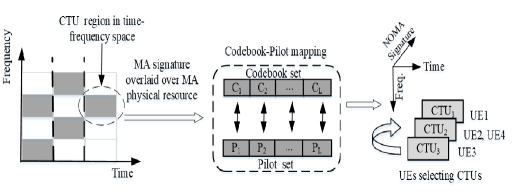
Figure 3: An illustration of CTU in a time-frequency space.

Unlike orthogonal resource allocation (i.e., each time-frequency resource can only be used by one UE), NOMA allows multiple UEs with different codebooks and pilot sequences to transmit over the same time-frequency resource, thus increasing the number of accessible UEs without expanding physical resources. However, a collision will occur when more than one UE selects the same codebook and pilot sequence (i.e. the same CTU).

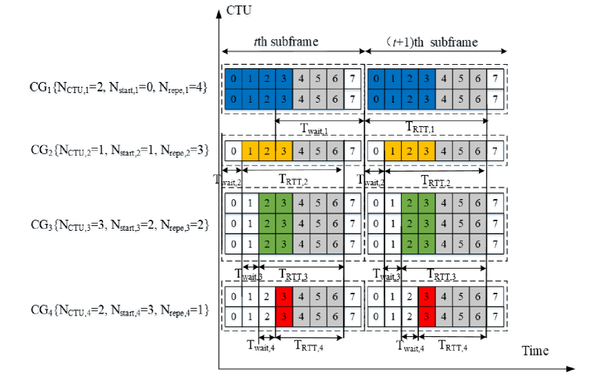
Figure 4: Multiple CGs (MCG) configurations with four CGs.

II-D Multiple Configured-Grants Grant-Free NOMA (MCG-GF-NOMA) Design

We consider the MCG-GF-NOMA system as shown in Fig. 4. The BS configures $N_{\rm CG}$ UL CGs for massive URLLC transmissions at each subframe. The UE chooses the configuration with the earliest starting point to transmit data. Each CG is consist of different resources in the CTU domains, and is associated with the following transmission parameters:

• Number of CTUs ($N_{\rm CTU}$)

• Starting slot within a subframe ($N_{\rm start}$)

• Number of repetitions ($N_{\rm repe}$)

• Number of slots in a subframe ($N_{\rm slot}$)

Without loss of generality, we consider that all the subframe has the same number of slots all the time, i.e., the $N_{\rm slot}$ is the same for each CG and each subframe. Thus, for ease of presentation, we represent each ${{\rm CG}_{i}}$ in the $t$th subframe by ${\rm CG}^{t}_{i}\{N^{t}_{{\rm CTU},i},N^{t}_{{\rm start},i},N^{t}_{{\rm repe},i}\}$. As illustrated in Fig. 4, ${\rm CG}^{t}_{1}\{2,0,4\}$, ${\rm CG}^{t}_{2}\{1,1,3\}$, ${\rm CG}^{t}_{3}\{3,2,2\}$, and ${\rm CG}^{t}_{4}\{2,3,1\}$ are four CGs in the $t$th subframe.

The main variables are summarized in Table I.

TABLE I: Notation Table

Symbol	Meaning	Symbol	Meaning
$N_{\rm UE}$	The number of static UEs	$R$	The coverage radius of the cell
$r$	The distance between an UE and the BS	$h$	The Rayleigh fading channel power gain
$\eta$	The path-loss exponent	$\mu$	The numerology factor
$N_{\rm sym}$	The number of OFDM symbols included in a slot	$N_{\rm slot}$	The number of slots within a subframe
$A$	The packets arrival rate	$p$	The Beta probability density
$T$	The duration of the bursty traffic	$L$	The number of pilot sequences over one RB
$F$	The number of time-frequency RBs	$N_{\rm CG}$	The number of CGs configured at each subframe
$N_{\rm CTU}$	The number of CTUs	${\cal N}_{\rm CTU}$	The set of the number of CTUs
$N_{\rm start}$	The starting slot within a subframe	${\cal N}_{\rm start}$	The set of the starting slot
$N_{\rm repe}$	The number of repetitions	$t$	The $t$th subframe
$T_{{\rm wait},i}^{t}$	The waiting time of the UE using ${{\rm CG}_{i}}$ at the $t$th subframe	$T_{{\rm RRT},i}^{t}$	The RTT time of the UE using ${{\rm CG}_{i}}$ at the $t$th subframe
$T_{{\rm laten},i}^{t}$	The latency of the UE using ${{\rm CG}_{i}}$ at the $t$th subframe	$T_{{\rm aver}}^{t}$	The average latency of the successfully served UEs at each subframe
$N_{{\rm suc},i}^{t}$	The successfully served UEs using ${{\rm CG}_{i}}$ at the $t$th subframe	${\cal N}_{{\rm IC},i}^{t}$	The set of idle CTUs for ${\rm CG}_{i}$ at the $t$th subframe
${\cal N}_{{\rm SC},i}^{t}$	The set of singleton CTUs for ${\rm CG}_{i}$ at the $t$th subframe	${\cal N}_{{\rm CC},i}^{t}$	The set of collision CTUs for ${\rm CG}_{i}$ at the $t$th subframe
${\cal N}_{f,{\rm SU},i}^{t}$	The set of UEs choosing the singleton CTUs for ${\rm CG}_{i}$ on the $f$th RB	${N}_{f,{\rm CU},i}^{t}$	The number of UEs choosing the collision CTUs for ${\rm CG}_{i}$ on the $f$th RB
$P$	The transmission power	$\sigma^{2}$	The noise power
$\gamma_{th}$	The received SINR threshold	$CG_{i}$	The $i$th CG in a subframe
$N_{{\rm CTU},{\rm SCG}}$	The configured CTU numbers for the SCG-GF-NOMA system	$T_{\rm RTT}$	The length of one round trip time
$T_{\rm wait}$	The length of waiting time	$T_{\rm laten}$	The latency of the successfully served UE
$T_{\rm aver}$	The average latency of the successfully served UEs in each subframe	$P_{s,f,i}$	The received power of the $s$th UE in the $n$th repetition of the CG $i$ on the $f$th RB

III Problem Analysis and Formulation

In a given subframe $t$, the BS preconfigured $N_{\rm CG}$ CGs for UEs to transmit their packets. The BS sends radio resource control (RRC) (for both type 1 and type 2 CG transmission) or downlink control information (DCI) (only for type 2 CG transmission) to activate or release the CG configurations[28]. As soon as the URLLC data arrives, a UE can choose the ${\rm CG}^{t}_{i}$ with the earliest starting point (i.e., the smallest $N^{t}_{{\rm start},i}$) to transmit data. Suppose that the UE choose the ${\rm CG}^{t}_{i}\{N^{t}_{{\rm CTU},i},N^{t}_{{\rm start},i},N^{t}_{{\rm repe},i}\}$, then the UE randomly choose a CTU from $N^{t}_{{\rm CTU},i}$ available CTUs and start transmit at slot $N^{t}_{{\rm start},i}$ for $N^{t}_{{\rm repe},i}$ repetitions. The BS decodes (D) each repetition independently and the transmission is successful when at least one repetition succeeds. After processing all the received $N^{t}_{{\rm repe},i}$ repetitions, the BS transmits the ACK/NACK feedback (F) to the UE. Considering the small packets of URLLC traffic, we set the packet transmission time as one TTI. The BS feedback time and the BS (UE) processing time are also assumed to be one TTI following our previous work [8]. The latency analysis and the reliability analysis for the MCG-GF-NOMA are described in the following.

III-A MCG-GF-NOMA Latency Analysis

In order to meet the low latency requirement for mURLLC, we consider that the active UE can only transmit for one round trip time (RTT). The RTT is the length time it takes for a data packet to be sent to a destination plus the time it takes for an acknowledgment of that packet to be received back at the origin. According to Fig. 4, the incurred latency of the UE using the $CG_{i}^{t}$ at the $t$th subframe includes two parts: the waiting time $T_{{\rm wait},i}^{t}$ and the RTT $T_{{\rm RTT},i}^{t}$. We obtain the RTT of the UE using $CG_{i}^{t}$ at the $t$th subframe as

$${T_{{\rm RRT},i}^{t}}=N^{t}_{{\rm repe},i}+3.$$ (5)

It should be noted that the UEs transmitting in ${\rm CG}_{i}^{t}$ come from those who received a packet after the start point of the ${\rm CG}_{i-1}^{t}$. Thus, the waiting time is the length time from the start point of the ${\rm CG}_{i-1}^{t}$ to the start point of the ${\rm CG}_{i}^{t}$. We derive the waiting time as

$${T_{{\rm wait},i}^{t}}=\tau^{i}-\tau^{i-1},$$ (6)

where

$$({\tau^{i-1}},{\tau^{i}})=$$ (7)

$$\left\{\begin{array}[]{l}(N_{\rm slot}\times(t-1)+N^{t}_{{\rm start},{i-1}},N_{\rm slot}\times(t-1)+N^{t}_{{\rm start},i}),\\ (i>1),\\ (0,0),\\ (i=1,t=1),\\ (N_{\rm slot}\times(t-2)+N^{t}_{{\rm start},N_{\rm CG}^{t-1}},N_{\rm slot}\times(t-2)+N_{\rm slot}),\\ (i=1,t>1).\end{array}\right.$$

According to (5), (6), and (7), we obtain the latency for ${\rm CG}^{t}_{i}$ as

$${T_{{\rm laten},i}^{t}}={T_{{\rm wait},i}^{t}}+{T_{{\rm RRT},i}^{t}}$$ (9)

$$=\left\{\begin{array}[]{l}N_{{\rm start},i}^{t}-N_{{\rm start},{i-1}}^{t}+N^{t}_{{\rm repe},i}+3,(i>1),\\ N^{t}_{{\rm repe},i}+3,(i=1,t=1),\\ N_{\rm slot}-N_{{\rm start},N_{\rm CG}^{t-1}}^{t}+N^{t}_{{\rm repe},i}+3,(i=1,t>1).\end{array}\right.$$ (13)

In order to compare the latency performance, we calculate the average latency of the successfully served UEs in each subframe as

$$T_{\rm aver}^{t}=\frac{{\sum\limits_{i}^{{N_{\rm CG}}}{T_{{\rm laten},i}^{t}\times N_{{\rm suc},i}^{t}}}}{{\sum\limits_{i}^{{N_{\rm CG}}}{N_{{\rm suc},i}^{t}}}},$$ (14)

where $N_{{\rm suc},i}^{t}$ is the successfully served UEs using the ${\rm CG}_{i}$ at the $t$th subframe and is obtained in the next subsection about reliability analysis.

III-B MCG-GF-NOMA Reliability Analysis

During each RTT, if the GF-NOMA procedure fails, the UE fails to be served and its packets will be dropped. The GF-NOMA fails if: ($i$) a CTU collision occurs when two or more UEs choose the same CTU (i.e., UE detection fails); or ($ii$) the SIC decoding fails (i.e., data decoding fails).

III-B1 CTU dectection

At each RTT, each active UE transmits its packets to the BS by randomly choosing a CTU from the earliest ${\rm CG}_{i}$. The BS can detect the UEs that have chosen different CTUs. However, if multiple UEs choose the same CTU, the BS cannot differentiate these UEs and therefore cannot decode the data. We categorize the CTUs from each ${\rm CG}_{i}$ into three types[14]:

• idle CTU: a CTU which has not been chosen by any UE;

• singleton CTU : a CTU chosen by only one UE;

• collision CTU : a CTU chosen by two or more UEs.

After collision detection at the $t$th subframe for the ${\rm CG}_{i}$, the BS observes the set of singleton CTUs ${\cal N}_{{\rm SC},i}^{t}$, the set of idle CTUs ${\cal N}_{{\rm IC},i}^{t}$, and the set of collision CTUs ${\cal N}_{{\rm CC},i}^{t}$ for each ${\rm CG}_{i}$.

III-B2 SIC decoding

After detecting the UEs that have chosen the singleton CTUs, the BS performs the SIC technique to decode the data of these UEs. Based on the NOMA principles, at each iterative stage of SIC, the BS first decodes the UE with the strongest received power and then subtracted the successfully decoded signal from the received signal (we assume perfect SIC the same as [14]). That is to say, the decoding order at the BS is in sequence to the received power. It worth noting that during the decoding, the UEs that transmit on different RBs do not interfere with each other due to the orthogonality, and only UEs that transmit on the same RB cause interference. Thus, in order to characterize the UEs transmitting with ${\rm CG}_{i}$ on the $f$th RB, we represent the ${\cal N}_{f,{\rm SU},i}^{t}$ as the set of UEs that have chosen the singleton CTUs for the ${\rm CG}_{i}$ on the $f$th RB, the ${N}_{f,{\rm SU},i}^{t}=\left|{\cal N}_{f,{\rm SU},i}^{t}\right|$ as the number of UEs that have chosen the singleton CTUs for the ${\rm CG}_{i}$ on the $f$th RB ($\left|\cdot\right|$ denotes the number of elements in any vector $\cdot$), and ${N}_{f,{\rm CU},i}^{t}$ as the number of UEs that have chosen the collision CTUs using the ${\rm CG}_{i}$ on the $f$th RB. We define the received power of the $s$th UE in the $n$th repetition of the ${\rm CG}_{i}$ on the $f$th RB as

$$P_{s,f,i}^{t}={{P}{h_{s,f,i}^{t}}{r_{s}}^{-\eta}},$$ (15)

where $P$ is the transmission power, $r$ is the Euclidean distance between the UE and the BS, $\eta$ is the path-loss attenuation factor, $h$ is the Rayleigh fading channel power gain from the UE to the BS.

Suppose that the received power obeys $P_{1,f,i}^{t}\geq P_{2,f,i}^{t}\geq...\geq P_{{N}_{f,{\rm SU},i}^{t}}^{t}$, the decoding order should be from the $1$st UE to the ${N}_{f,{\rm SU},i}$th UE. In each iterative stage of SIC decoding, the CTU with the strongest received power is decoded by treating the received powers of other CTUs over the same RB as the interference. Thus, at the $t$th subframe, in the $n$th repetition of the ${\rm CG}_{i}$ on the $f$th RB, the signal-to-interference-plus-noise ratio (SINR) of the $s$th stage of SIC decoding of the $s$th UE is derived as

$${\rm SINR}^{t}_{s,f,i}=\frac{{P_{s,f,i}^{t}}}{{\sum\limits_{m=s+1}^{{N}_{f,SU,i}^{t}}P_{m,f,i}^{t}+\sum\limits_{n^{\prime}=1}^{{N}_{f,CU,i}^{t}}P_{n^{\prime},f,i}^{t}+{\sigma^{2}}}},$$ (16)

where $\sigma^{2}$ is the noise power.

Each iterative stage of SIC decoding is successful when the SINR in that stage is larger than the SINR threshold, i.e., ${\rm SINR}^{t}_{s,f,i}\geq{\gamma_{th}}$. The SIC procedure stops when one iterative stage of the SIC fails or when there are no more signals to decode. The SIC decoding procedure for each ${\rm CG}_{i}$ is described in the following.

• Step 1: Start the $n$th repetition with the initial $n=1$, ${\cal N}_{f,{\rm SU},i}^{t}$, ${N}_{f,{\rm SU},i}^{t}$ and ${N}_{f,{\rm CU},i}^{t}$;

• Step 2: Decode the $s$th UE with the initial $s=1$ using (16);

• Step 3: If the $s$th UE is successfully decoded, put the decoded UE in set ${\cal N}_{f,{\rm suc},i}^{t}(n)$ and go to Step 4, otherwise go to Step 5;

• Step 4: If $s\leq{N}_{f,{\rm SU},i}^{t}$, do $s=s+1$, go to Step 2, otherwise go to Step 5;

• Step 5: SIC for the $n$th repetition stops;

• Step 6: If $n\leq N_{{\rm repe},i}$, do $n=n+1$, go to Step 1, otherwise go to the end.

Finally, the set of successfully served UEs using the ${\rm CG}_{i}$ on the $f$th RB at the $t$th subframe is derived as

$${\cal N}_{f,{\rm suc},i}^{t}=\bigcup\limits_{n=1}^{{N_{{\rm repe},i}}}{({{\cal N}_{f,{\rm suc},i}^{t}(n)})},$$ (17)

the set of the successfully served UEs using the ${\rm CG}_{i}$ at the $t$th subframe is obtained as

$${\cal N}_{{\rm suc},i}^{t}=\bigcup\limits_{f=1}^{{F^{t}}}{({{\cal N}_{f,{\rm suc},i}^{t}})},$$ (18)

and the set of the successfully served UEs at the $t$th subframe is obtained as

$${\cal N}_{{\rm suc}}^{t}=\bigcup\limits_{i=1}^{{N_{\rm CG}}}{({{\cal N}_{{\rm suc},i}^{t}})}.$$ (19)

Then, ${N}_{{\rm suc}}^{t}=\left|{{\cal N}_{{\rm suc}}^{t}}\right|$ is the number of successfully served UEs.

III-C Problem Formulation

In this work, we aim to tackle the problem of optimizing the MCG-GF-NOMA configuration defined by parameters ${\rm CG}^{t}_{i}\{N^{t}_{{\rm CTU},i},N^{t}_{{\rm start},i},N^{t}_{{\rm repe},i}\}$ for each subframe $t$. At each subframe $t$, the BS aims at maximizing a long-term objective $R_{t}$ related to the average number of UEs that have successfully send data with respect to the stochastic policy $\pi$ that maps the current observation history $O^{t}$ to the probabilities of selecting each possible parameters in $A^{t}$. This optimization problem (P1) can be formulated as:

$$({\rm P1}:) \max\limits_{\pi({A^{t}}|{{O^{t}}})}\quad\sum\limits_{k=t}^{\infty}{{\gamma^{k-t}}}{{\mathbb{E}}_{\pi}}[N_{\rm suc}^{k}]$$ (20)

$$s.t.\quad \sum\limits_{i=1}^{{N_{\rm CG}}}N^{t}_{{\rm CTU},i}=N^{t}_{{\rm CTU},{\rm SCG}},$$ (21)

$$N^{t}_{{\rm start},i}+N^{t}_{{\rm repe},i}+3=N_{\rm slot},\forall i\in[1,N_{\rm CG}],$$ (22)

$$N^{t}_{{\rm start},i}<N^{t}_{{\rm start},i+1}<N_{\rm slot}-3,\forall i\in[1,N_{\rm CG}],$$ (23)

where $\gamma\in[0,1)$ is the discount factor for the performance accrued in the future subframes, and $\gamma=0$ means that the agent just concerns the immediate reward. The CTU resource constraint in (21) is set to compare with the SCG-GF-NOMA scheme, where $N^{t}_{{\rm CTU},{\rm SCG}}$ is the configured CTU numbers for the SCG-GF-NOMA. That is to say, the MCG-GF-NOMA configuration uses the same frequency resources but overlap in time and have different starting points so they do not require the additional resources compared to the conventional SCG-GF-NOMA scheme. The latency constraint in (22) is set to satisfy the latency requirement. That is to say, the transmission must be completed in one subframe (1 ms). Otherwise, the packet will be dropped. The starting slot constraint in (23) is set to support different UL packet arrival times.

All these constraints yield a mixed-integer non-convex problem and, in general, there is no standard method for solving this kind of problem efficiently. Additionally, since the dynamics of the MCG-GF-NOMA system is Markovian over the continuous subframes, this is a Partially Observable Markov Decision Process (POMDP) problem that is generally intractable for the conventional convex optimization algorithms due to their limitation in overcoming the dynamic in the environment. Here, partial observation refers to that a BS can not fully know all the information of the communication environment, including, but not limited to, the channel conditions, the random collision process, and the traffic statistics. The search space is expanded as the number of parameters increases, which also makes the conventional gradient-based optimization techniques unsuitable. The deep reinforcement learning (DRL) is regarded as powerful tool to address complex dynamic control problems in POMDP. The reasons in choosing DQN are that: 1) the Deep Neural Network (DNN) function approximation is able to deal with several kinds of partially observable problems [29, 30]; 2) DQN has the potential to accurately approximate the desired value function while addressing a problem with very large state spaces; 3) DQN is with high scalability, where the scale of its value function can be easily fit to a more complicated problem; 4) a variety of libraries have been established to facilitate building DNN architectures and accelerate experiments, such as TensorFlow, Pytorch, Theano, Keras, and etc.. The goal of deploying and designing the MCG-GF-NOMA is for maximizing the long-term benefits, which falls into the field of the DRL algorithm for the reason that this algorithm can monitor the reward resulting from its actions and incorporate farsighted system evolution instead of myopically optimizing current benefits.

IV Proposed Optimization Solution

In this section, we propose a Cooperative Multi-Agent Double Deep Q-Network (CMA-DDQN) approach to tackle the problem (P1), which breaks down the selection in high-dimensional action space into multiple parallel sub-tasks.

The aim of the CMA-DDQN model is to enable the agent to carry out the optimal actions to maximize the long-term sum reward. The principle of the CMA-DDQN model is maximizing the long-term sum reward instead of aiming for maximizing the reward at a particular subframe. Thus, in the CMA-DDQN model, the selected action may not be the optimal choice for the current subframe, but the optimal choice for pursing long-term benefits. In this paper, the parameters configuration of MCG-GF-NOMA is considered as discrete, so the value-based RL algorithm is invoked. The state space, action space, reward function design of the proposed CMA-DDQN based algorithm are specified.

IV-A Reinforcement Learning Framework

To optimize the number of successfully served UEs in MCG-GF-NOMA system, we consider a RL-agent deployed at the BS to interact with the environment in order to choose appropriate actions progressively leading to the optimization goal. We define $S\in\cal S$, $A\in\cal A$, and $R\in\cal R$ as any state, action, and reward from their corresponding sets, respectively. At the beginning of each subframe $t$, the RL-agent first observes the current state $S^{t}$ corresponding to a set of previous observations ${U^{t^{\prime}}}$ for all prior subframes (${t^{\prime}=1,...,t-1}$) in order to select an specific action $A^{t}\in{\cal A}(S^{t})$. After carrying out the action $A^{t}$, the RL-agent transits to a new observed state $S^{t+1}$ and obtains a corresponding reward $R^{t+1}$ as the feedback from the environment, which is designed based on the new observed state $S^{t+1}$ and guides the agent to achieve the optimization goal. After enough iterations, the BS can learn the optimal policy that maximizes the long-term rewards.

At each subframe $t$, a Q-value is calculated based on the current state and previously taken actions. Thus, the state, action and Q-value is stored in a Q-function, $Q(S^{t},A^{t})$, which determines the decision policy $\pi$. The Q-value and Q-function are updated based on the current state, previously taken actions and the received reward by following the principle

$$Q(S^{t},A^{t})$$ (24)

$$=Q(S^{t},A^{t})+\lambda[R^{t+1}+\gamma\mathop{\max}\limits_{A\in{\cal A}}Q(S^{t+1},A)-Q(S^{t},A^{t})],$$

The detailed descriptions of the state, action and reward of problem (P1) are introduced as follows.

IV-A1 States in the Q-learning Model

In terms of the state space of the proposed CMA-DDQN model, it contains five parts: the number of the collision CTUs ${N_{\rm CC}^{t^{\prime}}}$, the number of the idle CTUs ${N_{\rm IC}^{t^{\prime}}}$, the number of the singleton CTUs ${N_{\rm SC}^{t^{\prime}}}$, the number of UEs that have been successfully detected and decoded under the latency constraint ${N_{\rm suc}^{t^{\prime}}}$, and the number of UEs that have been successfully detected but not successfully decoded ${N_{\rm fdec}^{t^{\prime}}}$.

IV-A2 Actions in the Q-learning Model

Practically, the MCG-GF-NOMA system is always configured with multiple CGs to serve UEs with random traffic. In this section, we study the problem (P1) of optimizing the resource configuration for multiple CGs each with parameters $CG^{t}=\{N^{t}_{{\rm CTU},i},N^{t}_{{\rm start},i},N^{t}_{{\rm repe},i}\}_{i=1}^{N_{\rm CG}}$, where $N^{t}_{{\rm CTU},i}$ is chosen from the set of the number of the CTUs ${\cal N}_{{\rm CTU}}$, $N^{t}_{{\rm start},i}$ is chosen from the set of the value of the repetitions ${\cal N}_{{\rm start}}$, and $N^{t}_{{\rm repe},i}$ is chosen from the set of the value of the repetitions ${\cal N}_{{\rm repe}}$. This joint optimization by configuring each parameter in each CG can improve the overall data transmission performance. However, considering multiple CGs results in the increment of observations space, which exponentially increases the size of state space. For example, the number of available actions corresponds to the possible combinations of configurations $\left|{\cal A}\right|=\prod\limits_{i=1}^{N_{\rm CG}}{(\left|{\cal N}_{{\rm CTU},i}\right|\times\left|{\cal N}_{{\rm start},i}\right|\times\left|{\cal N}_{{\rm repe},i}\right|)}$. To train Q-agent with this expansion, the requirements of time and computational resources greatly increase. In view of this, we revise the configured parameters by considering the constraints from (21) to (23).

Input: Set of number of CTUs ${\cal N}_{\rm CTU}$, Length of CTUs set ${N}_{\rm CTU}=\left|{\cal N}_{{\rm CTU}}\right|$, Number of configured CTUs for the SCG-GF-NOMA $N^{t}_{{\rm CTU},{\rm SCG}}$, Number of the configured CG at each subframe $N_{\rm CG}$.

Output: The set of actions for the number of CTUs configuration ${\cal A}_{\rm CTU}^{t}$

1Define set ${\cal A}_{\rm CTU}^{t}$;

2Generate the initial index matrix: $X\in{\mathbb{C}}^{1\times N_{\rm CG}}$ with all the elements equaling to 0;

3Generate the max index matrix: ${X}_{\rm max}\in{\mathbb{C}}^{1\times N_{\rm CG}}$ with all the elements equaling to $N_{\rm CTU}$;

4The total searching steps $S_{teps}=\prod\limits_{i=1}^{N_{\rm CG}}{{X}_{\rm max}[i]}$;

5for j $\leftarrow$ 1 to $S_{teps}$  do

6       if $\sum\limits_{i=1}^{N_{\rm CG}}{{\cal N}_{\rm CTU}[X[i]]}=N^{t}_{{\rm CTU},{\rm SCG}}$ then

7            Put action $A_{\rm CTU}^{t}=\{{\cal N}_{\rm CTU}[X[i]],\forall i\in\left[1,N_{\rm CG}\right]\}$ into the action set ${\cal A}_{\rm CTU}^{t}$;

8       end if

9      

10      for k $\leftarrow$ 1 to ${N}_{\rm CG}$ do

11             $X[-k]+=1$;

12            if $X[-k]\textless X_{\rm max}[-k]:$ break;

13            $X[-k]\%=X_{\rm max}[-k]$.

14       end for

15      

16 end for

Algorithm 1 Generate the set of actions for the number of CTUs configuration.

First, considering the CTU resource constraint $\sum\limits_{i=1}^{{N_{\rm CG}}}N^{t}_{{\rm CTU},i}=N^{t}_{{\rm CTU},{\rm SCG}}$ as presented in (21), we could obtain the action set ${\cal A}_{\rm CTU}^{t}$, which consists of the actions $A_{\rm CTU}^{t}\in{\cal A}_{\rm CTU}^{t}$ with $A_{\rm CTU}^{t}=\{{N_{{\rm CTU},1}^{t}},...,{N_{{\rm CTU},N_{\rm CG}}^{t}}\}$. To find all possible combinations of the number of CPUs for multiple CG configurations with the CTU resource constraint, we follow the Algorithm 1.

In addition, considering the starting slot constraint $N^{t}_{{\rm start},i}<N^{t}_{{\rm start},i+1}<N_{\rm slot}-3,\forall i\in[1,N_{\rm CG}]$ in (23), we could obtain the action set ${\cal A}_{\rm start}^{t}$, which consists of the actions $A_{\rm start}^{t}\in{\cal A}_{\rm start}^{t}$ with $A_{\rm start}^{t}=\{N_{{\rm start},1}^{t},...,N_{{\rm start},N_{\rm CG}}^{t}\}$. Similarly, following the Algorithm 1, we can get all possible combinations of the starting slots for multiple CG configurations with the starting slot constraint. Different from the CTU action set, in step 6, the constraint should be starting slot constraint.

According to the latency constraint in (22), we have $N^{t}_{{\rm repe},i}=N_{\rm slot}-3-N^{t}_{{\rm start},i},\forall i,$. Therefore, two actions set ${\cal A}_{\rm CTU}^{t}$ and ${\cal A}_{\rm start}^{t}$ is enough to characterize the multiple CG configurations defined by parameters ${\rm CG}^{t}_{i}\{N^{t}_{{\rm CTU},i},N^{t}_{{\rm start},i},N^{t}_{{\rm repe},i}\}$.

IV-A3 Reward Function in the Q-Learning Model

As the optimization goal is to maximize the number of the successfully served UEs under the latency constraint, we define the reward $R^{t+1}$ as

$$R^{t+1}=N_{\rm suc}^{t},$$ (25)

where ${N_{\rm suc}^{t}}$ is the number of UEs that have been successfully detected and decoded under the latency constraint.

IV-B Cooperative Multi-Agent DDQN Approach

When the number of actions and states is small, the RL algorithm can efficiently obtain the optimal policy. However, when a large number of actions and states exist, which will inevitably result in massive computation latency and severely affect the performance of the RL algorithm. To address this issue, DRL is introduced, where DRL can directly control the behavior of each agent and solve complex decision-making problems, through interaction with the environment[29, 30]. In addition, Multi-Agent RL (MA-RL) is introduced with centralized or decentralized rewards. In MA-RL with centralized rewards, all agents receive a common (central) reward, while in MA-RL with decentralized rewards, every agent obtains a distinct reward [31]. However, in MA-RL with decentralized rewards, all agents may compete with each other, i.e., agents may act in a selfish behavior for requiring the highest reward which may affect the global network performance. To convert this selfishness into cooperative behavior, the same reward may be assigned to all agents [32]. In this section, we apply the Cooperative Multi-Agent technique based DDQN (CMA-DDQN) to prevent the selfish behavior of agents.

The challenge of this approach is how to evaluate each action according to the common reward function. For each DQN agent, the received reward is corrupted by massive noise, where its own effect on the reward is deeply hidden in the effects of all other DQN agents. For instance, a positive action can receive a mismatched low reward due to other DQN agents’ negative actions. Fortunately, in our scenario, all DQN agents are centralized at the BS, which means that all DQN agents can have full information among each other. The CMA-DDQN algorithm utilizes the experience replay technique to enhance the convergence performance of RL. When updating the CMA-DDQN algorithm, mini-batch samples are selected randomly from the experience memory as the input of the neural network, which breaks down the correlation among the training samples. In addition, through averaging the selected samples, the distribution of training samples can be smoothed, which avoids the training divergence. We define $A^{t}_{x}$ as the action selected by the $x$th agent. Each $x$th agent is responsible for updating the value $Q(S^{t},A^{t}_{x})$ of action $A^{t}_{x}$ in state $S^{t}$, where the state variable ${{S^{t}}}=[A^{t-1},U^{t-1},A^{t-2},U^{t-2},...,A^{t-M_{o}},U^{t-M_{o}}]$ only includes information about the last $M_{o}$ RTTs. All agents receive the same reward $R^{t+1}$ at the end of each subframe.

Input: : Action space $\cal A$ and Operation Iteration I.

1Algorithm hyperparameters: learning rate $\lambda_{RMS}\in(0,1])$, discount rate $\gamma\in[0,1)$, $\epsilon$-greedy rate $\epsilon\in(0,1]$, target network update frequency $Y$;

2Initialization of replay memory $M$ to capacity $D$, the state-action value function $Q(S,A,{\bm{\theta}})$, the parameters of primary Q-network $\bm{\theta}$, and the target Q-network $\bm{\bar{\theta}}$;

3for Iteration $\leftarrow$ 1 to I do

4       Initialization of $S^{1}$ by executing a random action $A^{0}_{x}$;

5      for t $\leftarrow$ 1 to T do

6            

7            if $p_{\epsilon}<\epsilon$ Then select a random action $A^{t}_{x}$ from ${\cal A}_{x}$

8            else select ${A^{t}_{x}}=\mathop{\arg\max}\limits_{a\in{\cal A}_{x}}Q({S^{t}},A_{x}^{t},\bm{\theta}_{x})$.

9            The BS broadcasts $A^{t}_{x}$ and backlogged UEs attempt communication in the $t$th subframe;

10            The BS observes state $S^{t+1}$, and calculate the related reward $R^{t+1}$;

11            Store transition $(S^{t},A^{t}_{x},R^{t+1},S^{t+1})$ in replay memory $M_{x}$;

12            Sample random minibatch of transitions $(S^{t},A^{t}_{x},R^{t+1},S^{t+1})$ from replay memory $M_{x}$;

13            Perform a gradient descent step and update parameters $\bm{\theta}_{x}$ for $Q(S^{t},A_{x}^{t},{\bm{\theta}_{x}})$ using (IV-B);

14            Update the parameter $\bm{\bar{\theta}}=\bm{\theta}$ of the target Q-network every $Y$ steps.

15       end for

16      

17 end for

Algorithm 2 CMA-DQN Based MCG-GF-NOMA Uplink Resource Configuration

The DDQN agents are trained in parallel. Each agent $x$ parameterizes the action-state value function $Q(S^{t},A^{t}_{x})$ by using a function $Q(S^{t},A^{t}_{x},\bm{\theta}_{x})$, where $\bm{\theta}_{x}$ represents the weights matrix of a multiple layers DNN with fully-connected layers. The variables in the state $S^{t}$ is fed in to the DNN as the input; the Rectifier Linear Units (ReLUs) are adopted as intermediate hidden layers; while the output layer is consisted of linear units, which are in one-to-one correspondence with all available actions in $\cal A$. The online update of weights matrix $\bm{\theta}_{x}$ is carried out along each training episode by using DDQN[33]. Accordingly, learning takes place over multiple training episodes, where each episode consists of several RTT periods. In each RTT, the parameters $\bm{\theta}_{x}$ of the Q-function approximator $Q(S^{t},A^{t}_{x},\bm{\theta}_{x})$ are updated using RMSProp optimizer[34] as

$${\bm{\theta}^{t+1}_{x}}={\bm{\theta}^{t}_{x}}-{\lambda_{\mathrm{RMS}}}\nabla{L_{x}^{\mathrm{DDQN}}}({\bm{\theta}^{t}_{x}})$$ (26)

where $\lambda_{\mathrm{RMS}}\in(0,1]$ is RMSProp learning rate, $\nabla{L_{x}^{\mathrm{DDQN}}}({\bm{\theta}^{t}_{x}})$ is the gradient of the loss function ${L_{x}^{\mathrm{DDQN}}}({\bm{\theta}^{t}_{x}})$ used to train the state-action value function. The gradient of the loss function is defined as

$$\nabla{L_{x}^{\mathrm{DDQN}}}({\bm{\theta}^{t}_{x}})$$

$$={{\rm E}_{{S^{j}},{A^{j}_{x}},{R^{j+1}},{S^{j+1}}}}[({R^{j+1}}+\gamma\mathop{\mathop{\max}\limits_{a\in{\cal A}}\ Q({S^{j+1}},{A_{x}^{j}},{{\bar{\bm{\theta}}}^{t}_{x}})}$$ (27)

$$-Q({S^{j}},{A^{j}_{x}},{\bm{\theta}^{t}_{x}})){\nabla_{\bm{\theta}_{x}}}Q({S^{j}},{A^{j}_{x}},{\bm{\theta}^{t}_{x}})],$$

where the expectation is taken over the minibatch, which are randomly selected from previous samples $(S^{j},A^{j}_{x},S^{j+1},R^{j+1})$ for $j\in\{t-M_{r},...,t\}$ with $M_{r}$ being the replay memory size[29]. When $t-M_{r}$ is negative, it represents to include samples from the previous episode. Furthermore, $\bar{{\bm{\theta}}^{t}}$ is the target Q-network in DDQN that is used to estimate the future value of the Q-function in the update rule, and $\bar{\bm{\theta}}^{t}$ is periodically copied from the current value ${\bm{\theta}}^{t}$ and kept unchanged for several episodes.

Through calculating the expectation of the selected previous samples in minibatch and updating the ${\bm{\theta}^{t}}$ by (26), the DDQN value function $Q(s,a,\bm{\theta})$ can be obtained. The detailed CMA-DDQN algorithm is presented in Algorithm 2. We consider $\epsilon$-greedy approach to balance exploitation and exploration in the actor of the Q-Agent, where $\epsilon$ is a positive real number and $\epsilon<1$. In each subframe $t$, the Q-agent randomly generates a probability $P_{\epsilon}^{t}$to compare with $\epsilon$. Then, with the probability $\epsilon$, the algorithm randomly chooses an action from the remaining feasible actions to improve the estimate of the non-greedy action’s value. With the probability $1-\epsilon$, the algorithm exploits the current knowledge of the Q-value table to choose the action that maximizes the expected reward.

IV-C Computational Complexity

The approximate complexity of generating the set of actions for $X$ agents is $O(XS_{step}N_{CG})$, where $S_{step}$ represents the maximum iteration steps and $N_{CG}$ represents the element number checking and correcting. The training complexity for $X$ agents, one minibatch of $I$ episodes with $T$ time-steps until convergence results in computational complexity is of order $O(X^{2}S_{step}N_{CG}IT)$ in training phase. The structures of the value function approximator can also be specifically designed for RL agents with sub-tasks of significantly different complexity. However, there is no such requirement in our problem, so it will not be considered. DNN is a better value function approximator due to its efficiency and capability in solving high complexity problems.

V Simulation Results

In this section, we examine the effectiveness of our proposed MCG-GF-NOMA system with CMA-DDQN algorithm via simulation. We adopt the standard network parameters listed in Table II following[35], and hyperparameters for the DQN learning algorithm are listed in Table III. Without loss of generality, in the simulation, we focus on the mini-slots of $N_{\rm sym}=7$ OFDM symbols for transmissions using 60 kHz ($\mu=2$) SCS, which is in line with the main guidelines for 3GPP NR performance evaluations presented in [35].

TABLE II: Simulation Parameters

Parameters	Value
Numerology factor $\mu$	2
Number of OFDM symbols in a slot $N_{\rm sym}$	7
Path-loss exponent $\eta$	4
Noise power $\sigma^{2}$	-132 dBm
Transmission power $P$	23 dBm
The received SINR threshold $\gamma_{th}$	-10 dB
Duration of traffic $T$	1000 ms
The number of the configured CTUs for the SCG-GF-NOMA $N_{{\rm CTU},{\rm SCG}}$	64
The set of the number of CTUs ${\cal N}_{CTU}$	$\{8,16,24,32,40,48,56\}$
The set of the starting slot ${\cal N}_{start}$	$\{0,1,2,3,4\}$
The number of static UEs for low (high) traffic $N_{\rm UE}$	10000 (50000)
The number of time-frequency RBs $F$	4
Cell radius $R$	10 km
The number of slots within a subframe $N_{\rm slot}$	8

TABLE III: Learning Hyperparameters

Hyperparameters	Value
Learning rate $\lambda_{RMS}$	0.0001
Minimum exploration rate $\epsilon$	0.1
Discount rate $\gamma$	0.5
Minibatch size	32
Replay Memory	10000
Target Q-network update frequency	1000

All testing performance results are obtained by averaging over 1000 episodes. The BS is located at the center of a circular area with a 10 km radius, and the UEs are randomly located within the cell. The DQN is set with two hidden layers, each with 128 ReLU units. In the following, we present our simulation results of multiple CG configurations in MCG-GF-NOMA system.

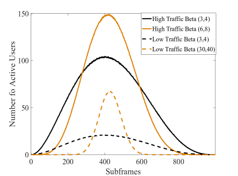
Figure 5: The real-time traffic load.

Throughout epoch, each UE has a bursty traffic profile (i.e., the time limited Beta profile defined in (4) with parameters (3, 4), (6, 8) or (30, 40)) that has a peak around the 400th subframe. The resulting average number of newly generated packets is shown in Fig. 5, where the dashed line represents the low traffic (LOW) and the solid line represents the high traffic (HIGH).

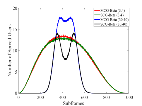
Figure 6: Average number of successfully served users in low traffic scenario.

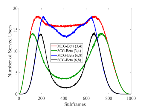
Figure 7: Average number of successfully served users in high traffic scenario.

Fig. 6 compares the number of successfully served UEs for MCG-GF-NOMA and SCG-GF-NOMA systems in low traffic scenario with parameters Beta(3, 4) and Beta(30, 40), respectively. Unless otherwise stated, we consider $N_{\rm CG}=5$ for the MCG-GF-NOMA system. It is obvious that the MCG-GF-NOMA can increase the successfully served UEs compared with the SCG-GF-NOMA, especially for the high bursty traffic peak (Beta(30, 40)), i.e., massive access simultaneously. Particularly, at the peak traffic, the number of successfully served UEs in the MCG-GF-NOMA system is circa two times more than that in the SCG-GF-NOMA system. However, when the bursty traffic is lower (Beta(3, 4)), this advantage of MCG is not obvious. This indicates that the MCG solution can ensure the massive access performance of GF-NOMA in a massive URLLC scenario.

Fig. 7 compares the number of successfully served UEs for MCG-GF-NOMA and SCG-GF-NOMA systems in high traffic scenario with parameters Beta(3,4) and Beta(6,8), respectively. We observe that at the peak traffic with parameter (3, 4), the number of successfully served UEs in the MCG-GF-NOMA system is circa four times more than that in the SCG-GF-NOMA system, while at the peak traffic with parameter (6, 8), the number of successfully served UEs in the MCG-GF-NOMA system is circa seven times more than that in the SCG-GF-NOMA system. This is in line with Fig. 6 that the MCG-GF-NOMA outperform the SCG-GF-NOMA for massive access scenario. It should be noted that the number of successfully served UEs for MCG-GF-NOMA with Beta (6, 8) decreases slightly at the peak traffic compared with that for MCG-GF-NOMA with Beta (3, 4). It indicates that with ever-increasing traffic, the ability of MCG-GF-NOMA will be limited, more efficient solution should be designed.

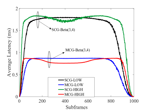
Figure 8: Average latency of successfully served users.

Fig. 8 compares the average latency of successfully served UEs in MCG-GF-NOMA and SCG-GF-NOMA systems with both high traffic and low scenarios with parameters Beta(3, 4), respectively. It is obvious that the MCG-GF-NOMA can decrease the average latency of successfully served UEs compared to the SCG-GF-NOMA, for both the high traffic and low traffic scenarios. In particular, the MCG-GF-NOMA system could almost decrease the latency by half compared with that in the SCG-GF-NOMA system. This indicates that the MCG solution can ensure the low latency performance of GF-NOMA in a massive URLLC scenario.

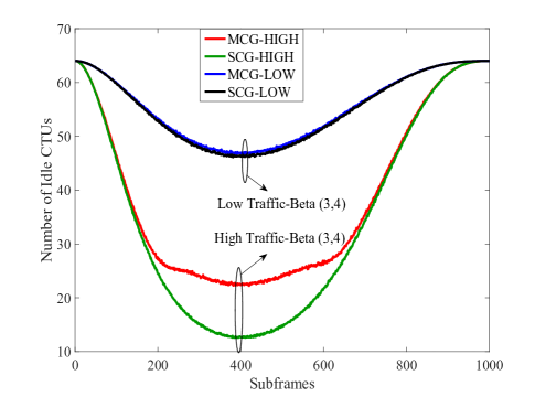
Figure 9: Average number of idle CTUs.

Fig. 9 and Fig. 10 compare the average number of idle and collision CTUs in MCG-GF-NOMA and SCG-GF-NOMA systems with both high traffic and low traffic scenarios with parameters Beta(3, 4), respectively. Combining with Fig. 6-Fig. 8, we observe that the multiple CGs solution can obtain better reliability and latency performance of MCG-GF-NOMA only by using smaller CTU resources than the SCG-GF-NOMA with the single CG, especially for the high traffic scenario. This is due to the fact that the MCG solution mitigates the heavy traffic backlog in the SCG-GF-NOMA system, where multiple UEs are active after the starting slot offset of one CG will wait for the next CG period to transmit the packet. Consequently, the collision events are mitigated in the MCG-GF-NOMA system.

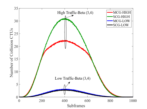
Figure 10: Average number of collision CTUs.

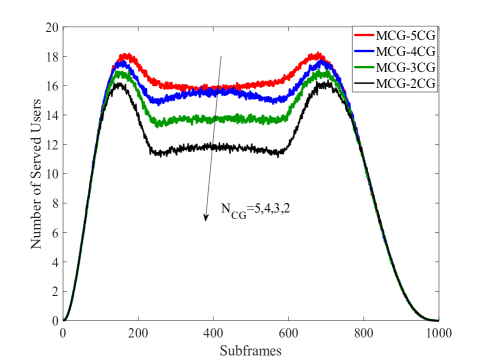
Figure 11: Average number of successfully served users in MCG-GF-NOMA with different numbers of configured-grants $N_{\rm CG}$.

Fig. 11 and Fig. 12 compare the average number of successfully served users and the average latency of successfully served users in the MCG-GF-NOMA system with high traffic for different numbers of CGs $N_{\rm CG}$, respectively. Unless otherwise stated, we consider bursty traffic parameter Beta(3, 4) for the MCG-GF-NOMA system. We observe that the average number of successfully served users increases, whereas the average latency of successfully served users decreases, with increasing the numbers of CGs $N_{\rm CG}$. The increased degree of the average number of successfully served users and the decreased degree of the average latency of successfully served users is largest at the peak traffic around the 400th subframe. This indicates that more CGs can improve the massive access performance of GF-NOMA in high traffic regions, which is in line of the descriptions of MCG-GF-NOMA in Section I.A. The MCG-GF-NOMA system could mitigate the collision events when multiple UEs are active and waiting for the CG period to transmit the packet. It should be noted that both the increased degree of the average number of successfully served users and the decreased degree of the average latency of successfully served users decrease with increasing the numbers of CGs $N_{\rm CG}$.

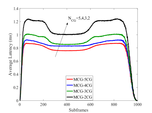
Figure 12: Average latency of successfully served users in MCG-GF-NOMA with different numbers of configured-grants $N_{\rm CG}$.

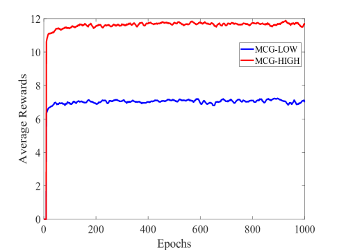
Figure 13: Average received reward.

In Fig. 13, we show the system convergence process of the proposed CMA-DDQN aided MCG-GF-NOMA schemes by plotting the average reward. It can be intuitively seen that the proposed framework has a fast convergence speed and the episode required for system convergence is very small.

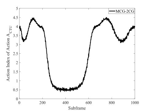
Figure 14: Action index of the action $A_{\rm CTU}$ in the action set ${\cal A}_{\rm CTU}$ for MCG-GF-NOMA with $N_{\rm CG}=2.$

Fig. 14 and Fig. 15 plot the action index of the action $A_{\rm CTU}$ in the action set ${\cal A}_{\rm CTU}$ and the action $A_{\rm start}$ in the action set ${\cal A}_{\rm start}$ for MCG-GF-NOMA systems in heavy traffic scenario with $N_{\rm CG}=2$, respectively. According to the Algorithm 1, we could obtain the action set ${\cal A}_{\rm CTU}=\{[8,56],[16,48],[24,40],[32,32],[40,24],[48,16],[56,8]\}$ as well as the action set ${\cal A}_{\rm start}=$ $\{[0,1],[0,2],[0,3],[0,4],[1,2],[1,3],[1,4],[2,3],[2,4],[3,4]\}$, which are sorted by the element in the matrix. In Fig. 14, we observe that the agent learns to adopt the action with a smaller number of CTUs for CG 1 and a larger number of CTUs for CG 2 around the peak traffic, e.g., $A_{\rm CTU}=[8,56]$. This is because the agent in the MCG-GF-NOMA scheme learns to sacrifice the successful transmission in CG 1 to alleviate the traffic congestion in CG 2 for heavy traffic regions to obtain a long-term reward. We also observe that the agent learns to adopt the action with the same number of CTUs for CG 1 and CG 2 around the low traffic, e.g., $A_{\rm CTU}=[32,32]$. This is because in a low traffic region with less traffic congestion the agent in the MCG-GF-NOMA scheme learns to guarantee the successful transmission in both the CG 1 and CG 2. Similarly, in Fig. 15, the agent learns to adopt the action with an earlier stating slot for CG 2 around the peak traffic, e.g., $A_{\rm start}=[0,1]$. This can guarantee the larger repetition value in CG2 to get high reliability.

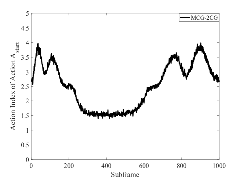
Figure 15: Action index of the action $A_{\rm start}$ in the action set ${\cal A}_{\rm start}$ for MCG-GF-NOMA with $N_{\rm CG}=2.$

VI Conclusion

In this paper, we proposed a novel MCG-GF-NOMA learning framework for attaining the long-term successfully served UEs under the latency constraint in mURLLC service, where bursty traffic of UEs was considered. We first designed and modeled the MCG-GF-NOMA system, where we characterize each CG using the parameters including the number of CTUs, the starting slot of each CG within a subframe, and the number of repetitions of each CG. We then characterized and analyzed the latency and reliability performances for each CG. We formulated the MCG-GF-NOMA resources configuration problem taking into account three constraints: 1) the CTU resource constraint is set to compare the MCG-GF-NOMA system with the SCG-GF-NOMA scheme; 2) the latency constraint is set to satisfy the latency requirement; and 3) the starting slot constraint is set to support various UL packet arrival times. Finally, we proposed a CMA-DDQN algorithm to balance the allocations of resources among MCGs so as to maximize the number of successful transmissions under the latency constraint, which breaks down the selection of high-dimensional parameters into multiple parallel sub-tasks with a number of DDQN agents cooperatively being trained to produce each parameter. Our results have shown that the MCG-GF-NOMA framework can improve the low latency and high realibity performances in a massive URLLC scenario. In detail, the number of successfully served UEs in the MCG-GF-NOMA system is circa four times more than that in the SCG-GF-NOMA system, and the latency of successfully served UEs in the MCG-GF-NOMA system is circa half of that in the SCG-GF-NOMA system in high traffic scenario. Our work will help to support the 3GPP evolution in terms of 1) the establishment of the theoretical foundation of MCG transmission procedure; and 2) PHY and MAC parameters configuration setup, evaluation, and optimization. Our proposed learning framework defined the observations, actions, and rewards to maximize long-term successfully served UEsunder the latency constrain, which can be standardized as the collected parameters from the environment. From the perspective of performance improvement, determining the retransmission or not can be optimized in the future by considering both the different latency constraints and the future traffic congestion. Furthermore, a promising future direction is to cooperatively optimize networks along with the UEs’ key performance indicators (KPIs), such as power consumption and transmission delay. Such multi-objective optimization is quite challenging and should be addressed in the future.

References

- [1] M. Series, “IMT vision-framework and overall objectives of the future development of IMT for 2020 and beyond,” Recommendation ITU, pp. 2083–0, Sep. 2015.
- [2] “Study on scenarios and requirements for next generation access technologies,” 3GPP, TS 38.913 v15.2.0, Jun. 2018.
- [3] X. Zhang, J. Wang, and H. V. Poor, “Statistical delay and error-rate bounded QoS provisioning for mURLLC over 6G CF M-MIMO mobile networks in the finite blocklength regime,” IEEE J. Sel. Areas Commun., pp. 1–1, Sep. 2020.
- [4] X. Zhang, J. Wang, and H. V. Poor, “Optimal resource allocations for statistical QoS provisioning to support mURLLC over FBC-EH-Based 6G THz wireless nano-networks,” IEEE J. Sel. Areas Commun, vol. 39, no. 6, pp. 1544–1560, Apr. 2021.
- [5] “5G; NR; physical layer procedures for data,” 3GPP TS 38.214 v15.9.0, Mar. 2020.
- [6] Y. Chen, A. Bayesteh, Y. Wu, B. Ren, S. Kang, S. Sun, Q. Xiong, C. Qian, B. Yu, Z. Ding, S. Wang, S. Han, X. Hou, H. Lin, R. Visoz, and R. Razavi, “Toward the standardization of non-orthogonal multiple access for next generation wireless networks,” IEEE Commun. Mag., vol. 56, no. 3, pp. 19–27, Mar. 2018.
- [7] T.-K. Le, U. Salim, and F. Kaltenberger, “An overview of physical layer design for ultra-reliable low-latency communications in 3GPP releases 15, 16, and 17,” IEEE Access, vol. 9, pp. 433–444, Dec. 2020.
- [8] Y. Liu, Y. Deng, M. Elkashlan, A. Nallanathan, and G. K. Karagiannidis, “Analyzing grant-free access for URLLC service,” IEEE J. Sel. Areas Commun., pp. 1–1, Aug. 2020.
- [9] M. Elbayoumi, M. Kamel, W. Hamouda, and A. Youssef, “NOMA-assisted machine-type communications in UDN: State-of-the-art and challenges,” IEEE Commun. Surveys Tutorials, vol. 22, no. 2, pp. 1276–1304, Mar. 2020.
- [10] M. B. Shahab, R. Abbas, M. Shirvanimoghaddam, and S. J. Johnson, “Grant-free non-orthogonal multiple access for IoT: A survey,” IEEE Commun. Surveys Tutorials, pp. 1–1, May. 2020.
- [11] “Enhanced UL configured grant transmissions for URLLC,” R1-1906151, 3GPP TSG RAN WG1 97, May. 2019.
- [12] A. Gunturu, V. S. Tijoriwala, and A. K. Reddy Chavva, “Optimal configured grant selection method for nr rel-16 uplink urllc,” in GLOBECOM 2020 - 2020 IEEE Global Communications Conference, Jan. 2020, pp. 1–6.
- [13] M. Shirvanimoghaddam, M. Condoluci, M. Dohler, and S. J. Johnson, “On the fundamental limits of random non-orthogonal multiple access in cellular massive IoT,” IEEE J. Sel. Areas Commun., vol. 35, no. 10, pp. 2238–2252, Jul. 2017.
- [14] R. Abbas, M. Shirvanimoghaddam, Y. Li, and B. Vucetic, “A novel analytical framework for massive grant-free NOMA,” IEEE Trans. Commun., vol. 67, no. 3, pp. 2436–2449, Mar. 2019.
- [15] Z. Ding, R. Schober, P. Fan, and H. V. Poor, “Simple semi-grant-free transmission strategies assisted by non-orthogonal multiple access,” IEEE Trans. Commun., vol. 67, no. 6, pp. 4464–4478, Mar. 2019.
- [16] J. Zhang, X. Tao, H. Wu, N. Zhang, and X. Zhang, “Deep reinforcement learning for throughput improvement of the uplink grant-free NOMA system,” IEEE Internet of Things Journal, vol. 7, no. 7, pp. 6369–6379, Feb. 2020.
- [17] M. V. da Silva, R. D. Souza, H. Alves, and T. Abrão, “A NOMA-Based Q-Learning random access method for machine type communications,” IEEE Wireless Commun. Lett., vol. 9, no. 10, pp. 1720–1724, Jun. 2020.
- [18] J. Liu, Z. Shi, S. Zhang, and N. Kato, “Distributed Q-Learning aided uplink grant-free NOMA for massive machine-type communications,” IEEE J. Sel. Areas Commun., vol. 39, no. 7, pp. 2029–2041, May. 2021.
- [19] “Physical channels and modulation,” 3GPP, TS 38.211 v15.8.0, Jan. 2020.
- [20] “Cellular system support for ultra-low complexity and low throughput Internet of Things (CIoT),” 3GPP, Sophia Antipolis, France, TR 45.820 V13.1.0,, Nov. 2015.
- [21] “Study on RAN improvements for machine-type communications,” 3GPP, TR 37.868 v11.0.0, Sep. 2011.
- [22] J. Navarro-Ortiz, P. Romero-Diaz, S. Sendra, P. Ameigeiras, J. J. Ramos-Munoz, and J. M. Lopez-Soler, “A survey on 5G usage scenarios and traffic models,” IEEE Commun. Surveys Tutorials, vol. 22, no. 2, pp. 905–929, Feb. 2020.
- [23] A. K. Gupta and S. Nadarajah, Handbook of beta distribution and its applications. CRC press, 2004.
- [24] N. Ye, H. Han, L. Zhao, and A.-H. Wang, “Uplink nonorthogonal multiple access technologies toward 5G: A survey,” Wireless Commun. Mobile Comput., vol. 2018, Jun. 2018.
- [25] K. Au, L. Zhang, H. Nikopour, E. Yi, A. Bayesteh, U. Vilaipornsawai, J. Ma, and P. Zhu, “Uplink contention based SCMA for 5G radio access,” in 2014 IEEE Globecom Workshops (GC Wkshps), May. 2014, pp. 900–905.
- [26] J. Zhang, L. Lu, Y. Sun, Y. Chen, J. Liang, J. Liu, H. Yang, S. Xing, Y. Wu, J. Ma, I. B. F. Murias, and F. J. L. Hernando, “PoC of SCMA-based uplink grant-free transmission in UCNC for 5G,” IEEE J. Sel. Areas Commun., vol. 35, no. 6, pp. 1353–1362, Jun. 2017.
- [27] A. C. Cirik, N. M. Balasubramanya, L. Lampe, G. Vos, and S. Bennett, “Toward the standardization of grant-free operation and the associated NOMA strategies in 3GPP,” IEEE Commun. Standards Mag., vol. 3, no. 4, pp. 60–66, Dec. 2019.
- [28] “Study on physical layer enhancements for NR ultra-reliable and low latency case (URLLC),” 3GPP, TR 38.824 v16.0.0, Mar. 2019.
- [29] R. S. Sutton and A. G. Barto, Reinforcement learning: An introduction. MIT press, 2018.
- [30] V. Mnih, K. Kavukcuoglu, D. Silver, A. A. Rusu, J. Veness, M. G. Bellemare, A. Graves, M. Riedmiller, A. K. Fidjeland, G. Ostrovski et al., “Human-level control through deep reinforcement learning,” nature, vol. 518, no. 7540, pp. 529–533, 2015.
- [31] D. Lee, N. He, P. Kamalaruban, and V. Cevher, “Optimization for reinforcement learning: From a single agent to cooperative agents,” IEEE Signal Process. Mag., vol. 37, no. 3, pp. 123–135, May. 2020.
- [32] L. Liang, H. Ye, and G. Y. Li, “Spectrum sharing in vehicular networks based on multi-agent reinforcement learning,” IEEE J. Sel. Areas Commun., vol. 37, no. 10, pp. 2282–2292, Aug. 2019.
- [33] H. Van Hasselt, A. Guez, and D. Silver, “Deep reinforcement learning with double q-learning,” arXiv preprint arXiv:1509.06461, Dec. 2015.
- [34] T. Tieleman and G. Hinton, “Lecture 6.5-rmsprop: Divide the gradient by a running average of its recent magnitude,” COURSERA: Neural Netw. Mach. Learn., vol. 4, no. 2, pp. 26–31, Oct. 2012.
- [35] “Study on new radio access technology-physical layer aspects,” 3GPP, TR 38.802 v14.0.0, Mar. 2017.