Nearly Optimal Quantum Algorithm for Estimating Multiple Expectation Values

Abstract

Many quantum algorithms involve the evaluation of expectation values. Optimal strategies for estimating a single expectation value are known, requiring a number of state preparations that scales with the target error $\varepsilon$ as $\mathcal{O}(1/\varepsilon)$. In this paper, we address the task of estimating the expectation values of $M$ different observables, each to within additive error $\varepsilon$, with the same $1/\varepsilon$ dependence. We describe an approach that leverages Gilyén et al.’s quantum gradient estimation algorithm to achieve $\mathcal{O}(\sqrt{M}/\varepsilon)$ scaling up to logarithmic factors, regardless of the commutation properties of the $M$ observables. We prove that this scaling is worst-case optimal in the high-precision regime if the state preparation is treated as a black box, even when the operators are mutually commuting. We highlight the flexibility of our approach by presenting several generalizations, including a strategy for accelerating the estimation of a collection of dynamic correlation functions.

Introduction

A fundamental task of quantum simulation is to perform an experiment in silico. Like traditional experimentalists, researchers using quantum computers will often be interested in efficiently measuring a collection of properties. For example, the electronic ground state problem is frequently cited as a motivation for quantum simulation of chemistry, but determining the ground state energy is only a starting point in most chemical applications. Depending on context, it may be essential to measure the dipole moment and polarizability, the electron density, the forces experienced by the classical nuclei, or various other quantities [1, 2]. Similarly, in condensed matter physics and beyond, correlation functions play a central role in the theory of quantum many-body phenomena due to their interpretability and measurability in the lab [3, 4].

In this letter, we consider the problem of accurately and efficiently estimating multiple properties from a quantum computation. We focus on evaluating the expectation values of a collection of $M$ Hermitian operators $\{O_{j}\}$ with respect to a pure state $\ket{\psi}$. We aim to evaluate each expectation value to within additive error $\varepsilon$ using as few calls as possible to a state preparation oracle for $\ket{\psi}$ (or its inverse). One simple approach is to repeatedly prepare $\ket{\psi}$ and projectively measure mutually commuting subsets of $\{O_{j}\}$. Alternatively, strategies based on amplitude estimation achieve a quadratic speedup with respect to $\varepsilon$ but entail measuring each observable separately [5, 6, 7]. A range of newer “shadow tomography” techniques use joint measurements of multiple copies of $\ket{\psi}$ to achieve polylogarithmic scaling with respect to $M$ at the expense of an unfavorable $1/\varepsilon^{4}$ scaling [8, 9, 10, 11]. In certain situations, randomized methods based on the idea of “classical shadows” of the state obtain $1/\varepsilon^{2}$ scaling while improving upon sampling protocols with deterministic measurement settings [12, 13]. We review these existing approaches in Appendix A and compare them to our new strategy in Table 1 and Appendix B.

Our main contribution is an algorithm that achieves the same $1/\varepsilon$ scaling as methods based on amplitude estimation, but also improves the scaling with respect to $M$ from $\widetilde{\mathcal{O}}(M)$ to $\widetilde{\mathcal{O}}(\sqrt{M})$, where the tilde in $\widetilde{\mathcal{O}}(\cdot)$ hides logarithmic factors. Our approach is to construct a function $f$ whose gradient yields the expectation values of interest and encode $f$ in a parameterized quantum circuit. We can then apply Gilyén et al.’s quantum algorithm for gradient estimation [14] to obtain the desired scaling. The following theorem formalizes our result.

Theorem 1.

Let $\{O_{j}\}$ be a set of $M$ Hermitian operators on $N$ qubits, with spectral norms $\|O_{j}\|\leq 1$ for all $j$. There exists a quantum algorithm that, for any $N$-qubit quantum state $\ket{\psi}$ prepared by a unitary $U_{\psi}$, outputs estimates $\widetilde{o_{j}}$ such that $|\widetilde{o_{j}}-\bra{\psi}O_{j}\ket{\psi}|\leq\varepsilon$ for all $j$ with probability at least $2/3$, using $\widetilde{\mathcal{O}}(\sqrt{M}/\varepsilon)$ queries to $U_{\psi}$ and $U_{\psi}^{\dagger}$, along with $\widetilde{\mathcal{O}}(\sqrt{M}/\varepsilon)$ gates of the form controlled-$e^{-ixO_{j}}$ for each $j$, for various values of $x$ with $|x|\in\mathcal{O}(1/\sqrt{M})$.

As we show in Corollary 3, this query complexity is worst-case optimal (up to logarithmic factors) in the high-precision regime where $\varepsilon\in(0,\frac{1}{3\sqrt{M}})$. After establishing this lower bound for our problem, we review the gradient algorithm of Ref. 14 and present the proof of Theorem 1. We then discuss several extensions of our approach, including a strategy for estimating multiple dynamic correlation functions and a method that handles observables with arbitrary norms (or precision requirements) based on a generalization of the gradient algorithm.

	Comm.	Non-comm.	$k$-RDM
Sampling	$\mathcal{O}(\frac{\log M}{\varepsilon^{2}})$	$\widetilde{\mathcal{O}}(\frac{M}{\varepsilon^{2}})$	$\widetilde{\mathcal{O}}(\frac{N^{k}}{\varepsilon^{2}})$ [13]
Amp. Est. [6]	$\widetilde{\mathcal{O}}(\frac{M}{\varepsilon})$	$\widetilde{\mathcal{O}}(\frac{M}{\varepsilon})$	$\widetilde{\mathcal{O}}(\frac{N^{2k}}{\varepsilon})$
Shadow Tom. [11]	$\mathcal{O}(\frac{\log M}{\varepsilon^{4}})$	$\mathcal{O}(\frac{\log{M}}{\varepsilon^{4}})$	$\mathcal{O}(\frac{k\log{N}}{\varepsilon^{4}})$
Gradient	$\widetilde{\mathcal{O}}(\frac{\sqrt{M}}{\varepsilon})$	$\widetilde{\mathcal{O}}(\frac{\sqrt{M}}{\varepsilon})$	$\widetilde{\mathcal{O}}(\frac{N^{k}}{\varepsilon})$

Table 1: A comparison of the (worst-case) complexities, in terms of state preparation oracle queries, of different approaches for measuring multiple observables. We consider three applications: estimating the expectation values of $M$ commuting or non-commuting observables, and determining the fermionic $k$-RDM of an $N$-mode system. Here, $\varepsilon$ denotes the additive error to which each quantity is estimated. We compare strategies based on naive sampling, amplitude estimation, and shadow tomography to our gradient-based approach. We cite the specific works used to determine these complexities, including the Pauli-specific shadow protocol of Ref. 11. Note that methods based on sampling and shadow tomography also work under a weaker input model where only copies of the state are provided.

Lower Bounds

In Ref. 15, Apeldoorn proved a lower bound for a task that is essentially a special case of our quantum expectation value problem. We explain how a lower bound for our problem can be obtained as a corollary. Their results are expressed in terms of a particular quantum access model for classical probability distributions:

Definition 1 (Sample oracle for a probability distribution).

Let $\mathbf{p}$ be a probability distribution over $M$ outcomes, i.e., $\mathbf{p}\in[0,1]^{M}$ with $\|\mathbf{p}\|_{1}=1$. A sample oracle $U_{\mathbf{p}}$ for $\mathbf{p}$ is a unitary operator that acts as

$$U_{\mathbf{p}}:\ket{0}\ket{0}\mapsto\sum_{j=1}^{M}\sqrt{p_{j}}\ket{j}\otimes\ket{\phi_{j}},$$ (1)

where the $\ket{\phi_{j}}$ are arbitrary normalized quantum states.

We rephrase Lemma 13 of Ref. 15 below. Here and throughout this paper, we count queries to a unitary oracle $U$ and to its inverse $U^{\dagger}$ as equivalent in cost.

Theorem 2 (Lemma 13, Ref. 15 (rephrased)).

Let $M$ be a positive integer power of $2$ and let $\varepsilon\in(0,\frac{1}{3\sqrt{M}})$. There exists a known matrix $A\in\{-1,+1\}^{M\times M}$ such that the following is true. Suppose $\mathcal{A}$ is an algorithm that, for every probability distribution $\mathbf{p}$, accessed via a sample oracle $U_{\mathbf{p}}$, outputs (with probability at least $2/3$) a $\mathbf{\tilde{q}}$ such that $\|A\mathbf{p}-\mathbf{\tilde{q}}\|_{\infty}\leq\varepsilon$. Then $\mathcal{A}$ must use $\Omega({\sqrt{M}}/{\varepsilon})$ queries to $U_{\mathbf{p}}$ in the worst case.

We can use this theorem to derive the following corollary, establishing the near-optimality of the algorithm in Theorem 1 in certain regimes.

Corollary 3.

Let $M$ be a positive integer power of $2$ and let $\varepsilon\in(0,\frac{1}{3\sqrt{M}})$. Let $\mathcal{A}$ be any algorithm that takes as an input an arbitrary set of $M$ observables $\{O_{j}\}$. Suppose that, for every quantum state $\ket{\psi}$, accessed via a state preparation oracle $U_{\psi}$, $\mathcal{A}$ outputs estimates of each $\expectationvalue{O_{j}}{\psi}$ to within additive error $\varepsilon$ (with probability at least $2/3$). Then, there exists a set of observables $\{O_{j}\}$ such that $\mathcal{A}$ applied to $\{O_{j}\}$ must use $\Omega({\sqrt{M}}/{\varepsilon})$ queries to $U_{\psi}$.

Proof.

Assume for the sake of contradiction that for any $\{O_{j}\}$ and $U_{\psi}$, the algorithm $\mathcal{A}$ uses $o(\sqrt{M}/\varepsilon)$ queries to $U_{\psi}$ to estimate every $\bra{\psi}O_{j}\ket{\psi}$ to within error $\varepsilon$ (with success probability at least $2/3$). For any sample oracle $U_{\mathbf{p}}$ of the form in Eq. (1), consider the state

$$\ket{\psi(U_{\mathbf{p}})}\coloneqq\sum_{j=1}^{M}\sqrt{p_{j}}\Big{(}\bigotimes_{i=1}^{M}\ket{\frac{1-A_{ij}}{2}}\Big{)}\otimes\ket{j}\otimes\ket{\phi_{j}}.$$ (2)

A quick computation verifies that the $i$-th entry of the vector $A\mathbf{p}$ is equal to $\expectationvalue{Z_{i}}{\psi(U_{\mathbf{p}})}$, where $Z_{i}$ denotes the Pauli $Z$ operator acting on the $i$-th qubit. Since the matrix $A$ is known, it is clear that $\ket{\psi(U_{\mathbf{p}})}=U_{A}(I\otimes U_{\mathbf{p}})\ket{0}$ for a known unitary $U_{A}$:

$$U_{A}=\sum_{j}\big{(}\bigotimes_{i=1}^{M}X_{i}^{\delta_{A_{ij},-1}}\big{)}\otimes\outerproduct{j}{j}\otimes\mathbb{I}.$$ (3)

Therefore, we can apply algorithm $\mathcal{A}$ with $O_{j}=Z_{j}$ for $j\in\{1,\cdots,M\}$ and $U_{\psi}=U_{A}(\mathbb{I}\otimes U_{\mathbf{p}})$. By our assumption, this constitutes an algorithm that for every $U_{\mathbf{p}}$, estimates each entry of $A\mathbf{p}$ to within error $\varepsilon$ using $o(\sqrt{M}/\varepsilon)$ queries to $U_{\mathbf{p}}$, contradicting Theorem 2, and completing the proof. ∎

Background on Gilyén et al.’s gradient algorithm

Our framework for simultaneously estimating multiple expectation values uses the improved quantum algorithm for gradient estimation of Gilyén, Arunachalam, and Wiebe (henceforth, Gilyén et al.) [14]. Gilyén et al. built on earlier work by Jordan [16], which demonstrated an exponential quantum speedup for computing the gradient in a particular black-box access model. Specifically, Jordan’s algorithm uses one query to a binary oracle (see Appendix C) for a function $f$, along with phase kickback and the quantum Fourier transform, to obtain an approximation of the gradient $\nabla f$.

While we defer a technical discussion of Gilyén et al.’s algorithm to Appendix C (and refer the reader also to Ref. 14), we give a brief, colloquial description of their algorithm here. It is helpful to review their definition for a probability oracle,

Definition 2 (Probability oracle).

Consider a function $f:\mathbb{R}^{M}\rightarrow[0,1]$. A probability oracle $U_{f}$ for $f$ is a unitary operator that acts as

$$U_{f}: \ket{\bm{x}}\ket{\bm{0}}\mapsto$$ (4)

$$\ket{\bm{x}}\left(\sqrt{f(\bm{x})}\ket{1}\ket{\phi_{1}(\bm{x})}+\sqrt{1-f(\bm{x})}\ket{0}\ket{\phi_{0}(\bm{x})}\right),$$

where $\ket{\bm{x}}$ denotes a discretization of the variable $\bm{x}$ encoded into a register of qubits, $\ket{\bm{0}}$ denotes the all-zeros state of a register of ancilla qubits, and $\ket{\phi_{0}(\bm{x})}$ and $\ket{\phi_{1}(\bm{x})}$ are arbitrary quantum states.

Gilyén et al. show how such a probability oracle can be used to encode a finite-difference approximation to a directional derivative of $f$ in the phase of an ancilla register, e.g., a first-order approximation is implemented by

$$A_{f^{\prime}_{1}}:\ket{\bm{x}}\ket{\bm{0}}\mapsto e^{i\left(f\left(\bm{x}\right)-f\left(\bm{-x}\right)\right)}\ket{\bm{x}}\ket{\bm{0}}.$$ (5)

As in Jordan’s original algorithm, a quantum Fourier transform can then be used to extract an approximate gradient from the phases accumulated on an appropriate superposition of basis states. By using higher-order finite-difference formulas, Gilyén et al. are able to estimate the gradient with a scaling that is optimal (up to logarithmic factors) for a particular family of smooth functions. We restate the formal properties of their algorithm in the theorem below.

Theorem 4 (Theorem 25, Ref. 14 (rephrased)).

Let $\varepsilon$, $c\in\mathbb{R}_{+}$ be fixed constants, with $\varepsilon\leq c$. Let $M\in\mathbb{Z}_{+}$ and $\bm{x}\in\mathbb{R}^{M}$. Suppose that $f:\mathbb{R}^{M}\rightarrow\mathbb{R}$ is an analytic function such that for every $k\in\mathbb{Z}_{+}$, the following bound holds for all $k$-th order partial derivatives of $f$ at $\bm{x}$ (denoted by $\partial_{{\bm{\alpha}}}f(\bm{x})$): $|\partial_{{\bm{\alpha}}}f(\bm{x})|\leq c^{k}k^{\frac{k}{2}}$. Then, there is a quantum algorithm that outputs an estimate $\widetilde{\bm{g}}\in\mathbb{R}^{M}$ such that $\|\nabla f(\bm{x})-\widetilde{\bm{g}}\|_{\infty}\leq\varepsilon$, with probability at least $1-\delta$. This algorithm makes $\widetilde{\mathcal{O}}(c\sqrt{M}\log(M/\delta)/\varepsilon)$ queries to a probability oracle for $f$.

Expectation values via the gradient algorithm

To construct our algorithm and prove Theorem 1, we build a probability oracle for a function whose gradient encodes the expectation values of interest and apply the quantum algorithm for the gradient.

Proof of Theorem 1.

We begin by defining the parameterized unitary

$$U(\bm{x})\coloneqq\prod_{j=1}^{M}e^{-2ix_{j}O_{j}}$$ (6)

for $\bm{x}\in\mathbb{R}^{M}$. The derivative of this unitary with respect to $x_{\ell}$ is

$$\frac{\partial U}{\partial x_{\ell}}=-2i\Bigg{(}\prod_{j=1}^{\ell}e^{-2ix_{j}O_{j}}\Bigg{)}O_{\ell}\Bigg{(}\prod_{k=\ell+1}^{M}e^{-2ix_{k}O_{k}}\Bigg{)}.$$ (7)

We are interested in the expectation of the $O_{j}$ with respect to the state $\ket{\psi}$, so we define the following function $f$:

$$f(\bm{x})\coloneqq-\frac{1}{2}\mathrm{Im}[\bra{\psi}U(\bm{x})\ket{\psi}]+\frac{1}{2}.$$ (8)

Using Eq. (7), we have

$$\frac{\partial f}{\partial x_{\ell}}\Bigg{|}_{\bm{x}=\bm{0}}=\expectationvalue{O_{\ell}}{\psi}.$$ (9)

Therefore, the gradient $\nabla f(\bm{0})$ is precisely the collection of expectation values of interest.

Now, we verify that $f$ satisfies the conditions of Theorem 4. Observe that $f$ is analytic and that the $k$-th order partial derivative of $f$ with respect to any collection of indices $\alpha\in\{1,\dots,M\}^{k}$ takes the form

$$\partial_{\alpha}f(\bm{x})=(-2)^{k-1}{\rm Im}(i^{k}\expectationvalue{V(\bm{x},{\bm{\alpha}})}{\psi}),$$ (10)

for some operator $V(\bm{x},\alpha)$ which depends on both $\alpha$ and $\bm{x}$. Note that $V$ is a product of terms which are either unitary, or from $\{O_{j}\}$. Since $\|O_{j}\|\leq 1$ for all $j$, we have $\|V\|\leq 1$, and therefore $|\partial_{\alpha}f(\bm{0})|\leq 2^{k-1}$ for all $k$ and $\alpha$. By setting $c=2$, we satisfy the derivative conditions of Theorem 4.

To construct a probability oracle for $f$ (see Definition 2), we need a quantum circuit that encodes $f(\bm{x})$ into the amplitudes of an ancilla. We construct such a circuit using the Hadamard test for the imaginary component of $\bra{\psi}U(\bm{x})\ket{\psi}$ [17, 18]. Let

$$F(\bm{x})\coloneqq\big{(}H\otimes\mathbb{I}\big{)}\big{(}\textsc{c-}U(\bm{x})\big{)}\big{(}S^{\dagger}H\otimes U_{\psi}\big{)},$$ (11)

where $H$ denotes the Hadamard gate, $\textsc{c-}U(\bm{x})$ the $U(\bm{x})$ gate controlled on the first qubit, and $S\coloneqq\ket{0}\!\!\bra{0}+i\ket{1}\!\!\bra{1}$ the phase gate. Applied to $\ket{0}\otimes\ket{\bm{0}}$, this circuit encodes $f(\bm{x})$ in the amplitudes with respect to the computational basis states of the first qubit:

$$F(\bm{x})\ket{0}\otimes\ket{\bm{0}}= \sqrt{f(\bm{x})}\ket{1}\otimes\ket{\phi_{1}(\bm{x})}+$$ (12)

$$\sqrt{1-f(\bm{x})}\ket{0}\otimes\ket{\phi_{0}(\bm{x})},$$

for some normalized states $\ket{\phi_{0}(\bm{x})}$ and $\ket{\phi_{1}(\bm{x})}$ (see Appendix D for more details). Note that $F(\bm{x})$ uses a single call to the oracle $U_{\psi}$.

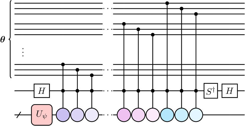
Figure 1: Schematic depiction of the quantum circuit for $U_{f}$, the probability oracle for the function $f(\bm{x})$ defined in Eq. (13). The top registers encode the ($n=3$ bit in this case) binary representations of $x_{1},x_{2},\cdots,x_{M}$. The ancilla qubit whose amplitudes encodes $f(\bm{x})$ (cf. Eq. (11)) is indicated below the $\bm{x}$ registers. The final line represents the $N$-qubit system register. The gates that act on the system register with colored circles represent the doubly-controlled time evolution by the various observables. Estimating the expectation values of the $M$ observables $\{O_{j}\}$ requires executing this circuit and its inverse $\widetilde{\mathcal{O}}(\sqrt{M}/\varepsilon)$ times.

All that remains is to add quantum controls to the rotations in $F(\bm{x})$, so that $F(\bm{x})$ is controlled on a register encoding $\bm{x}$. Specifically, we consider the unitary

$$U_{f}\coloneqq\sum_{\bm{k}\in G_{n}^{M}}\outerproduct{\bm{k}}{\bm{k}}\otimes F(\bm{k}x_{\max}),$$ (13)

where $G_{n}^{M}$ is a set of $2^{nM}$ points distributed in an $M$-dimensional unit hypercube, with $n=\mathcal{O}(\log(1/\varepsilon))$, and $x_{\max}$ is a rescaling factor. The values of $x_{\max}$ and $n$ are chosen to satisfy the requirements of the gradient algorithm (see Appendix C). Here, $\ket{\bm{k}}=\ket{k_{1}}\dots\ket{k_{M}}$ for $\bm{k}\in G_{n}^{M}$ denotes the basis state storing the binary representation of $\bm{k}$ in $M$ $n$-qubit index registers. The controlled time evolution operator for each $O_{j}$ can be implemented efficiently as a product of $n$ controlled-$e^{-ixO_{j}}$ gates with exponentially spaced values of $x$, each controlled on the appropriate qubit of the $j$th index register. We illustrate an example of such a $U_{f}$ in Figure 1.

$U_{f}$ is a probability oracle for the function $f$, and each call to $U_{f}$ involves a single call to the state preparation oracle $U_{\psi}$. Theorem 4 then implies that with probability at least $2/3$, every component of the gradient of $f$, and hence all of the expectation values $\bra{\psi}O_{j}\ket{\psi}$, can be estimated to within an error $\varepsilon$ using $\widetilde{\mathcal{O}}(\sqrt{M}/\varepsilon)$ queries to $U_{f}$. The complexity in terms of the controlled time evolutions follows from multiplying the number of controlled time evolutions required for each query to $U_{f}$, i.e., $\mathcal{O}(\log(M/\varepsilon))$ per observable, by the total number of queries, i.e., $\widetilde{\mathcal{O}}(\sqrt{M}/\varepsilon)$. As discussed in Appendix C, we have $x_{\max}\in\mathcal{O}(1/\sqrt{M})$ as a consequence of the details of the proof of Theorem 4 in Ref. 14. This completes the proof of Theorem 1. ∎

Furthermore (see Appendix C), the space complexity of the gradient algorithm is the same as that of the probability oracle up to an additive logarithmic factor . Therefore, our algorithm uses $\mathcal{O}(M\log(1/\varepsilon)+N)$ qubits.

Discussion

In this letter, we considered the problem of simultaneously estimating the expectation values of multiple observables with respect to a pure state $\ket{\psi}$. We presented an algorithm that uses $\widetilde{\mathcal{O}}(\sqrt{M}\varepsilon^{-1})$ applications of $U_{\psi}$ and its inverse, where $M$ denotes the number of observables and $\varepsilon$ the target error, and $U_{\psi}$ is a unitary that prepares $\ket{\psi}$. We explained how a lower bound on a closely related problem posed in Ref. 15 implies that, for algorithms given black-box access to $U_{\psi}$, this query complexity is worst-case optimal up to logarithmic factors when $\varepsilon\in(0,\frac{1}{3\sqrt{M}})$. In fact, our algorithm affirmatively resolves an open question from Ref. 15 regarding the achievability of this bound for the simultaneous estimation of classical random variables . These results imply that the optimal cost for expectation value estimation can become exponentially worse with respect to $M$ when one demands a scaling that goes as $\varepsilon^{-1}$ instead of $\varepsilon^{-2}$. Furthermore, the instances used in establishing our lower bounds involve a set of mutually commuting observables, implying that commutativity isn’t necessarily helpful when one demands $\varepsilon^{-1}$ scaling.

We presented a comparison with other approaches for the estimation of expectation values in Table 1, which we elaborate on in Appendix A and Appendix B. For example, we find that our algorithm is capable of estimating each element of the $k$-body fermionic reduced density matrix ($k$-RDM) of an $N$-mode system to within error $\varepsilon$ using $\widetilde{\mathcal{O}}(N^{k}/\varepsilon)$ state preparation queries. This offers an unconditional asymptotic speedup compared to existing methods when $\varepsilon=o(N^{-k/3})$. This may be particularly useful in practical applications where we wish to achieve a fixed error in extensive quantities by measuring the $1$ or $2$-RDM and summing $\Omega(N)$ elements.

Our gradient-based approach to estimating expectation values can be extended to other properties. For example, consider the task of evaluating a collection of two-point dynamic correlation functions. These functions take the form

$$C_{A,B}(t)\coloneqq\expectationvalue{U(0,t)A^{\dagger}U(t,0)B}{\psi},$$ (14)

where $A$ and $B$ are some simple operators and $U(t,t^{\prime})$ is the time evolution operator that maps the system from time $t^{\prime}$ to time $t$. These correlation functions are often directly accessible in experiment, as in the case of angle-resolved photoemission spectroscopy [3], and are also central to hybrid quantum-classical methods based on dynamical mean-field theory [21, 22, 23]. In Appendix E, we explain how a generalization of our approach can reduce the number of state preparations required for estimating a collection of these correlation functions.

Although we focused on quantifying the number of state preparation oracle queries, we also considered two other complexity measures. Our approach requires time evolution by each of the $M$ observables. The total duration of time evolution required scales as $\widetilde{\mathcal{O}}(M/\varepsilon)$. We also need an additional $\widetilde{\mathcal{O}}(M\log(1/\varepsilon))$ qubits, although we can modify our approach to trade off between space and query complexities (see  Appendix F). When we are interested in simultaneously estimating $O(N)$ expectation values, the asymptotic scaling of the space complexity is only logarithmically larger than that of storing the system itself. This is the case in a variety of contexts, for example, in the evaluation of the momentum distribution [24]. In other situations, the space overhead may be more substantial, though the capability of modern simulation algorithms to use so-called “dirty ancilla” (temporarily borrowing qubits in an arbitrary state) may offset this challenge in some contexts [25, 26, 27]. As a concrete example, we consider the double-factorized simulation of the electronic structure Hamiltionian proposed in Ref. 26. Von Burg et al. find that the time complexity of their simulation algorithm can be minimized by using $\widetilde{\mathcal{O}}(N^{3/2})$ qubits for data-lookup. These same qubits could be used by our algorithm for expectation value estimation to parallelize the measurement of $\widetilde{\mathcal{O}}(N^{3/2})$ observables, offering a $\widetilde{\mathcal{O}}(N^{3/4})$ asymptotic speedup without any additional qubit overhead.

Another potential reason for modifying our approach arises when the observables of interest have different norms, or when the desired precision varies. In Appendix G, we consider addressing this situation by measuring certain observables using our strategy and measuring others using a sampling-based method. In Appendix H, we take a different approach, and generalize Gilyén et al.’s gradient estimation algorithm to accommodate functions whose gradient components are not necessarily uniformly bounded. This allows us to simultaneously estimate the expectation values of observables $\{O_{j}\}$ with arbitrary norms $\|O_{j}\|$ (possibly greater than $1$) using $\widetilde{\mathcal{O}}(\sqrt{\sum_{j}\|O_{j}\|^{2}}/\varepsilon)$ queries. By rescaling the individual observables we can then also vary how precisely we estimate each expectation value, thereby extending Theorem 1 to the most general setting.

Our focus has been on the asymptotic scaling of our approach, but it will also be desirable to understand the actual costs. Performing a fault-tolerant resource estimate and a comparison against other measurement strategies in the context of a practical application would be a useful line of future work. It is possible that our approach could be modified to obtain a further speedup by taking advantage of the structure of the states and/or observables for particular problems of interest. Another potentially fruitful direction would be to explore extensions of the gradient algorithm to yield quantum algorithms for the Hessian or even higher-order derivatives.

Extracting useful information from a quantum computation, especially a quantum simulation, is a bottleneck for many applications. This is especially true in fields such as quantum chemistry and materials science, where it may be necessary to couple high-level quantum calculations with coarser approximations at other length scales in order to describe macroscopic physical phenomena. We expect that our gradient-based approach to the estimation of expectation values will be a useful tool and a starting point for related approaches to other problems.

Appendix A Prior work on expectation value estimation

This letter focuses on the task of estimating the expectation value of multiple observables with respect to a pure state $\ket{\psi}$. Motivated by settings where the cost of state preparation is the dominant factor, we mainly quantify the resources required in an oracle model where we count the number of calls to the state preparation unitary and its inverse. To provide concrete motivation for this cost model and for the task in general, consider the example where our state of interest is the unknown ground state of some second-quantized electronic structure Hamiltonian under the Jordan-Wigner transformation. In this case, the state preparation step is expected to be tractable under certain assumptions but relatively expensive, even using modern methods (e.g., by applying the ground state preparation algorithms of Ref. 28, 29 in conjunction with state-of-the-art techniques for block-encoding the Hamiltonian [25, 26]). At the same time, the observables of interest may be especially simple (e.g., the elements of a fermionic reduced density matrix). We discuss the situation where the cost of state preparation does not necessarily dominate, and the possible trade-offs available in the context of our approach, in Appendix F

Let $U_{\psi}$ denote the unitary which prepares $\ket{\psi}$ from the $\ket{0}$ state, and let $\{O_{j}\}$ be a collection of $M$ Hermitian operators. For the sake of simplifying the comparison with existing approaches, we make the additional assumption in this section that the $O_{j}$ are also unitary, though this requirement could be relaxed by using techniques based on block-encodings [7]. As in the main text, our goal is to minimize the number of calls to $U_{\psi}$ and $U_{\psi}^{\dagger}$ required to obtain estimates $\widetilde{o_{j}}$ of the $M$ expectation values $\bra{\psi}O_{j}\ket{\psi}$ such that

$$|\widetilde{o_{j}}-\expectationvalue{O_{j}}{\psi}|\leq\varepsilon$$ (15)

for all $j\in\{1,\dots,M\}$ with probability at least $2/3$. We note that some of the methods we compare against are usable under a weaker input model, where the algorithm is merely provided copies of $\ket{\psi}$ rather than access to a state preparation oracle.

A straightforward approach is to repeatedly prepare the state $\ket{\psi}$ and simultaneously measure as many of the operators as possible on each copy. To this end, consider dividing the $M$ operators into $G$ groups of mutually commuting terms. Then

$$C=\mathcal{O}\left(\frac{G\log M}{\varepsilon^{2}}\right)$$ (16)

calls to $U_{\psi}$ suffice to estimate the $M$ expectation values. This can be accomplished by simultaneously diagonalizing the operators within each group and measuring in the common eigenbasis when this is tractable, or by performing phase estimation on the operators within each group using the same copy of $\ket{\psi}$. The outcomes are then averaged over repeated iterations. One key advantage of this approach is that, although it has poor scaling with the target error $\varepsilon$, it does not scale polynomially with $M$, and instead scales with $G$, which could be considerably smaller than $M$. In practice, optimally grouping and sampling the observables may be challenging and can introduce substantial overheads not captured by the query complexity (e.g., the classical cost of finding optimal groupings [30, 31] and of simultaneous diagonalization, the quantum gate complexity of implementing basis change unitaries corresponding to the common eigenbasis, or of phase estimation).

Alternatively, using a strategy based on amplitude estimation [5], we can estimate expectation values with a scaling proportional to $\varepsilon^{-1}$ [6, 7]. Amplitude estimation, as originally implemented in Ref. 6, allows for the estimation of the expectation value $\langle\psi|U|\psi\rangle$ of a unitary operator $U$. estimation algorithm of Ref. 6. The amplitude estimation algorithm works by performing phase estimation on the Szegedy walk operator,

$$S=-RURU^{{\dagger}},\hskip 14.22636ptR=1-2|\psi\rangle\langle\psi|.$$ (17)

One can verify that the operator $S$ is diagonal in the subspace spanned by $|\psi\rangle$ and $U|\psi\rangle$, with eigenvalues $e^{\pm ix}$ for $x=\cos^{-1}(2|\langle\psi|U|\psi\rangle|^{2}-1)$. Phase estimation on $S$ therefore allows for the determination of $|\expectationvalue{\psi}{U}|^{2}$ up to an accuracy $\varepsilon$ with a cost that scales as $1/\varepsilon$. Information about the phase may be regained by repeating this for different variants of $U$ controlled by an ancilla qubit. One can generalize this approach to the estimation of the expectation value of an arbitrary observable $O$ by providing a $U$ that block encodes $O$ [7]. Unfortunately, this algorithm does not generalize in a straightforward way to the task of estimating multiple expectation values, even when the operators commute (beyond the strategy of treating each one separately). As a consequence, estimating all $M$ expectation values using amplitude estimation requires

$$C=\widetilde{\mathcal{O}}\left({\frac{M}{\varepsilon}}\right)$$ (18)

calls to $U_{\psi}$ and $U_{\psi}^{\dagger}$. While this leads to an asymptotic advantage over naive sampling in some settings, it fails to do so in cases where $G/\varepsilon=o(M)$.

These two well-known strategies are complemented by the more recent body of work that began with Aaronson’s definition of the “shadow tomography” problem, the problem of estimating the expectation value of many two-outcome measurements given multiple copies of some input state [8]. Ref. 8 proposes a computationally expensive protocol for this task that achieves scaling logarithmic in the number of two-outcome measurements $M$ and proportional to $\varepsilon^{-4}$, up to logarithmic factors. Ref. 12 put forward an alternative protocol based on randomized measurement that also scales logarithmically in $M$, and improves the scaling with $\varepsilon$ from $\widetilde{\mathcal{O}}(\varepsilon^{-4})$ to $\widetilde{\mathcal{O}}(\varepsilon^{-2})$ at the expense of limiting the types of observables that can be treated efficiently (i.e., without introducing a scaling polynomial in the Hilbert space dimension). A series of additional works have offered improvements and variations on both the randomized measurement approach [13, 32, 33], and the more general approaches based on gentle measurements [9, 10, 11].

In this work, we are primarily concerned with the high-precision regime, and aim to achieve $\widetilde{\mathcal{O}}(\varepsilon^{-1})$ scaling. It is natural to ask whether it is possible to simultaneously achieve an asymptotic cost that is logarithmic in the number of observables $M$ and linear (up to logarithmic factors) in $\varepsilon^{-1}$ using our input model, where the input state is unknown and accessed via a black-box state preparation unitary. In Corollary III in the main text, we point out that recent results preclude this, showing that the desired $\varepsilon^{-1}$ scaling in the precision necessarily comes at the cost of a square root dependence on $M$ for certain collections of observables. On the other hand, Ref. 15 provides an example of a collection of operators—namely, projectors onto orthogonal states—where this scaling is achievable.

Appendix B Applications

In this appendix, we apply our method to three illustrative cases and consider the potential for asymptotic speedups over alternative approaches. As in the main text, we focus on quantifying the cost with respect to the number of state preparation oracle queries. We note that some of the approaches we compare against (namely, methods based on sampling and shadow tomography) are usable under a weaker access model, where copies of the state are provided rather than queries to the state preparation oracle.

A major application of these ideas is the measurement of the fermionic $k$-body reduced density matrices ($k$-RDMs) of a particular pure state. The $k$-RDM of a pure state $\ket{\chi}$ with support on $N$ fermionic modes is a tensor specified by the $N^{2k}$ “matrix elements” of the form $\bra{\chi}a^{\dagger}_{p_{1}}\cdots a^{\dagger}_{p_{k}}a_{p_{k+1}}\cdots a_{p_{2k}}\ket{\chi}$, where the $2k$ indices $p_{j}$ take values ranging over the $N$ modes. The $1$- and $2$- RDMs are particularly important, being sufficient to determine the expected energy of a state and many other properties of interest [34].

The $\mathcal{O}(N^{2k})$ terms in the $k$-RDM can be divided into $\Omega(N^{k})$ groups of $\mathcal{O}(N^{k})$ mutually commuting operators [35]. This allows for each of the terms to be estimated to within a precision $\varepsilon$ by a simple sampling procedure with a query complexity of $\widetilde{\mathcal{O}}(N^{k}/\varepsilon^{2})$ [13]. The asymptotic scaling with $\varepsilon$ can be quadratically improved (see Appendix A by applying amplitude estimation to learn each component individually with the requisite error, leading to a query complexity of $\widetilde{\mathcal{O}}(N^{2k}/\varepsilon)$. Some shadow tomography protocols scale better with respect to $N$ and $k$ than either of these approaches, at the expense of scaling with $\varepsilon^{-4}$ [11, 8, 9, 10]. In particular, the technique described in Ref. 11 can estimate the $k$-RDM at a cost that scales as $\mathcal{O}(k\log(N)/\varepsilon^{4})$ by estimating the expectation values of all degree $2k$ majorana operators under the Jordan-Wigner transformation to within a precision $\varepsilon$ and using these values to reconstruct the $k$-RDM. Our gradient-based algorithm’s scaling of $\widetilde{\mathcal{O}}(N^{k}/\varepsilon)$ for this application follows directly from Theorem 1 in the main text. In terms of the number of state preparation oracle queries, our method thus strictly improves upon sampling and amplitude estimation for this application, and provides an asymptotic advantage over all prior approaches for learning the $k$-RDM when $\varepsilon\in o(N^{-k/3})$. This might naturally occur when we are interested in obtaining estimates of some extensive quantities to within a fixed precision by summing estimates of $O(N)$ local observables.

For the case where we wish to apply our ideas to compute the expectation values of $M$ mutually commuting observables with respect to a state $\ket{\psi}$, the potential benefit still exists, but the trade-offs are less favorable. In this case, commutation allows every expectation value to be measured on a single copy of $\ket{\psi}$. Sampling then yields $\widetilde{\mathcal{O}}(\log(M)/\varepsilon^{2})$ scaling, where the logarithmic dependence on $M$ arises from the application of concentration inequalities together with the union bound to guarantee that all of the $M$ expectation values are estimated to within $\varepsilon$ simultaneously (with some constant probability of success). This is in contrast to the $\widetilde{\mathcal{O}}(\sqrt{M}/\varepsilon)$ scaling of Theorem 1 in the main text. This does not contradict the optimality of our approach in the high-precision regime, due to the requirement that $\varepsilon<1/(3\sqrt{M})$ in Theorem 2 and Corollary 3 in the main text. Inside this region of applicability, sampling has at best the same scaling as our algorithm. The trade-offs between sampling and quantum gradient approaches, as well as algorithms that blend the two, are discussed in Appendix F

Another simple case to consider is one where we wish to measure $M$ observables that all fail to commute. Then it is clear that our approach offers an unconditional speedup when compared with approaches based on sampling and amplitude estimation (in terms of the number of state preparation oracle queries). It is still possible in this case to obtain a better scaling with respect to $M$ by employing shadow tomography [8, 9, 10, 11]. We provided a brief discussion of these approaches in Appendix A To summarize, these strategies require a number of state preparation oracle calls (actually, copies of the state) that scale logarithmically (or poly-logarithmically) with $M$ at the cost of scaling with $\varepsilon^{-4}$. When $\varepsilon=o(M^{-1/6})$ our approach has a favorable asymptotic scaling in terms of the state preparation oracle query complexity.

We note that these shadow tomography protocols are limited in other ways that may ultimately lead to a gate complexity advantage for our method for particular applications, even when the query complexity advantage is absent. Some such protocols, such as the one in Ref. 8, have gate complexities that scale exponentially in one or more relevant parameters. Others, such as the one in Ref. 11, are computationally efficient but only apply to limited sets of operators (Pauli observables in the case of Ref. 11). The proposal of Ref. 9 avoids both of these obstacles but returns a representation of the state in terms of a quantum circuit that must itself be prepared and measured to obtain the expectation values of interest. In some cases, it might be fruitful to apply our measurement techniques to the state whose preparation circuit is learned by this latter proposal.

Appendix C Further background on Gilyén et al.’s quantum algorithm for gradient estimation

In this appendix, we restate a few of the important definitions used in the main theorem which summarizes the performance of the quantum algorithm for the gradient (Theorem 4 in the main text of this work, Theorem 25 in Ref. 14). We also point out some of the details of the gradient algorithm relevant to our consideration of costs beyond the phase oracle complexity that are not included in the main statement of the theorem. We refer the interested reader to Ref. 14 for a rigorous analysis and further information about the implementation.

In Theorem 4 of the main text, we referred to the probability oracle access model for $f$. We recall this definition here, as well as the definitions for the phase oracle access model from Ref. 14 and the binary oracle access model used in Jordan’s original gradient algorithm [16].

Definition 3 (Probability oracle).

Consider a function $f:\mathbb{R}^{M}\rightarrow[0,1]$. A probability oracle $U_{f}$ for $f$ is a unitary operator that acts as

$$U_{f}:\ket{\bm{x}}\ket{\bm{0}}\mapsto\ket{\bm{x}}\left(\sqrt{f(\bm{x})}\ket{1}\ket{\phi_{1}(\bm{x})}+\sqrt{1-f(\bm{x})}\ket{0}\ket{\phi_{0}(\bm{x})}\right),$$ (19)

where $\ket{\bm{x}}$ denotes a discretization of the variable $\bm{x}$ encoded into a register of qubits, $\ket{\bm{0}}$ denotes the all-zeros state of a register of ancilla qubits, and $\ket{\phi_{0}(\bm{x})}$ and $\ket{\phi_{1}(\bm{x})}$ are arbitrary quantum states.

Definition 4 (Phase oracle).

Consider a function $f:\mathbb{R}^{M}\rightarrow\mathbb{R}$. A phase oracle $A_{f}$ for $f$ is a unitary operator that acts as

$$A_{f}:\ket{\bm{x}}\ket{\bm{0}}\mapsto e^{if(\bm{x})}\ket{\bm{x}}\ket{\bm{0}},$$ (20)

where $\ket{\bm{x}}$ denotes a discretization of the variable $\bm{x}$ encoded into a register of qubits and $\ket{\bm{0}}$ denotes the all-zeros state of a register of ancilla qubits.

Definition 5 (Binary oracle).

Consider a function $f:\mathbb{R}^{M}\rightarrow\mathbb{R}$. For some precision parameter $\varepsilon>0$, an $\varepsilon$-accurate binary oracle $B_{f}$ for $f(\bm{x})$ is a unitary operator that acts as

$$B_{f}:\ket{\bm{x}}\ket{\bm{0}}\mapsto\ket{\bm{x}}|\widetilde{f}(\bm{x})\rangle,$$ (21)

where $\ket{\bm{x}}$ denotes a discretization of the variable $\bm{x}$ encoded into a register of qubits, $\ket{\bm{0}}$ denotes the all-zeros state of a register of ancilla qubits, and $\widetilde{f}(\bm{x})$ denotes a fixed-point binary number such that $|f(\bm{x})-\widetilde{f}(\bm{x})|\leq\varepsilon$.

While we referred to the probability oracle access model in our Theorem 4 (in the main text), the original Theorem 25 of Ref. 14 described the gradient algorithm purely in terms of the phase oracle access model. However, they also show how we can efficiently obtain a probability oracle from a phase oracle.

Theorem 5 (Theorem 14, Ref. 14).

Let $U_{f}$ be a probability oracle for a function $f(\bm{x})$. For any $\varepsilon\in(0,\frac{1}{3})$, we can implement an $\varepsilon$-approximate phase oracle $\widetilde{A}_{f}$ such that

$$\|\widetilde{A}_{f}\ket{\psi}\ket{\bm{0}}-A_{f}\ket{\psi}\ket{\bm{0}}\|\leq\varepsilon$$ (22)

for all input states $\ket{\psi}$, where $A_{f}$ denotes an exact phase oracle for $f$. This implementation uses $\mathcal{O}(\log({1}/{\varepsilon}))$ invocations of the probability oracle $U_{f}$ (or its inverse) and $\mathcal{O}(\log\log({1}/{\varepsilon}))$ additional ancilla qubits beyond those required by $U_{f}$.

Therefore, we can regard calls to a phase oracle for $f$ as equivalent to calls to a probability oracle for $f$ up to logarithmic factors. More technically, the actual implementation of the gradient algorithm requires the use of a modified phase oracle known as a fractional query phase oracle. A fractional query phase oracle is defined in the same way as the phase oracle of Definition 4, except that it has an additional parameter $s\in[-1,1]$ which rescales the argument of the exponential. Fortunately, Ref. 14 explains how a fractional phase oracle can be naturally arrived at from a probability oracle in a theorem closely related to Theorem 5 (essentially by applying a rotation to rescale the amplitude $\sqrt{f(\bm{x})}$ of $\ket{1}$ in Eq. (19) to $\sqrt{sf(\bm{x})}$, before converting to a phase oracle).

The statement of Theorem 1 in the main text gives the cost of the gradient estimation algorithm in terms of the number of calls to a probability oracle. Similarly, for our expectation value estimation algorithm, we mainly focus on quantifying the cost in terms of oracle complexity (in particular, the number of queries to the state preparation oracle). However, we also wish to describe some of the secondary costs that we encounter in our algorithm, so it is useful to note a few additional details about the gradient estimation algorithm.

A secondary cost we might consider is the amount of time evolution required for each observable. From the proof of Theorem 25 in Ref. 14, we know that the phase oracle is queried at uniform superpositions of points within a series of $M$-dimensional boxes and that the largest such box has a side length of

$$x_{\max}\coloneqq rm,$$ (23)

where $r$ is defined implicitly by the equation

$$r^{-1}\coloneqq 9cm\sqrt{M}(81\cdot 8\cdot 42\pi cm\sqrt{M}/\varepsilon)^{1/(2m)},$$ (24)

and $m$ is a positive integer,

$$m\coloneqq\big{\lceil}\log(c\sqrt{M}/\varepsilon)\big{\rceil}.$$ (25)

Here, $c$ is the same fixed constant as that introduced in Theorem 4 in the main text for bounding the partial derivatives of $f$. As a consequence of these expressions, we have that the largest side length shrinks as $M$ increases. Specifically, $x_{\max}=\mathcal{O}(1/\sqrt{M})$. Calls to the phase oracle are generated using calls to the probability oracle and its inverse over the same input parameters (see the proof of Theorem 14 in Ref. 14, stated above as Theorem 5 for convenience) and the box size for the probability oracle directly determines the amount of time evolution by each observable. Therefore, for each probability oracle query, we require at most $\mathcal{O}(1/\sqrt{M})$ units of time evolution by each observable.

The other substantial secondary cost to consider is the space complexity. The probability oracle $U_{f}$ for our expectation value algorithm can be implemented using $N+1+Mn$ qubits, where $n=\mathcal{O}(\log(1/\varepsilon))$. The additive cost of $N+1$ comes from the system register and the ancilla for the Hadamard test. The $Mn$ terms is due to the need for $M$ $n$-bit ancilla registers to prepare a superposition over states indexing the $2^{nM}$ points in the hypercube $G_{n}^{M}$. To be specific, this hypercube is composed of the Cartesian product of $M$ copies of the set $G_{n}$, defined as

$$G_{n}\coloneqq\left\{j/2^{n}-1/2+1/2^{n+1}:j\in\left\{0,1,...,2^{n}-1\right\}\right\}.$$ (26)

The logarithmic scaling of $n$ with $1/\varepsilon$ comes from the precision requirements of the gradient algorithm (see the definition of $n$ in Theorem 21 in Ref. 14 and note that the factors of $\ell\in\{-m,-m+1,...,m\}$ that appear in the argument of the oracle in Theorem 25 can be accounted for by compiling a family of $2m+1$ related phase/probability oracles on grids of varying size). The conversion from a probability oracle to an $\varepsilon^{\prime}$-approximate phase oracle requires only $\mathcal{O}(\log\log(1/\varepsilon^{\prime}))$ additional ancilla. The gradient algorithm nominally requires storing $\mathcal{O}(\log(M/\delta))$ copies of each value and performing a coherent median finding step, but this can be performed classically for our purposes, eliminating the need for an additional multiplicative factor of $\mathcal{O}(\log M)$ in the number of qubits. We therefore have that the space complexity for our estimation algorithm is $N+1+Mn+\mathcal{O}(\log\log(Q/\varepsilon))$, where $n=\mathcal{O}(\log(1/\varepsilon))$ (see above) and $Q=\widetilde{\mathcal{O}}(\sqrt{M}/\varepsilon)$ is the number of queries we make to the phase oracle.

The oracle, gate, and qubit complexities of our algorithm for estimating the expectation values of a general collection of observables (with arbitrary norms) are analyzed in Appendix H see SI Theorem 6 for an explicit statement.

Appendix D Additional details regarding gradient-based expectation value estimation

In the main text, we claimed that the circuit $F(\bm{x})$, defined in Equation 11 as

$$F(\bm{x})\coloneqq\big{(}H\otimes\mathbb{I}\big{)}\big{(}\textsc{c-}U(\bm{x})\big{)}\big{(}S^{\dagger}H\otimes U_{\psi}\big{)},$$ (27)

encodes the function

$$f(\bm{x})=-\frac{1}{2}{\rm Im}\Bigg{[}\expectationvalue{\prod_{j=1}^{M}e^{-2ix_{j}O_{j}}}{\psi}\Bigg{]}+\frac{1}{2}$$ (28)

in the following way:

$$F(\bm{x})\ket{0}\otimes\ket{\bm{0}}=\sqrt{f(\bm{x})}\ket{1}\otimes\ket{\phi_{1}(\bm{x})}+\sqrt{1-f(\bm{x})}\ket{0}\otimes\ket{\phi_{0}(\bm{x})},$$ (29)

where $\ket{\phi_{0}(\bm{x})}$ and $\ket{\phi_{1}(\bm{x})}$ are some arbitrary normalized quantum states. While checking this identity directly is burdensome, it is easy to verify its correctness by observing that $F(\bm{x})$ is the circuit that performs the the Hadamard test for the imaginary component of $\expectationvalue{\prod_{j=1}^{M}e^{-2ix_{j}O_{j}}}{\psi}$ [17, 18]. That is, the expectation value of the Pauli $Z$ operator on the ancilla qubit with respect to the state $F(\bm{x})\ket{0}\otimes\ket{\bm{0}}$ is, by construction, equal to ${\rm Im}\Big{[}\expectationvalue{\prod_{j=1}^{M}e^{-2ix_{j}O_{j}}}{\psi}\Big{]}$.

Let $c_{0}$ and $c_{1}$ be defined implicitly by the following expression,

$$F(\bm{x})\ket{0}\otimes\ket{\bm{0}}=c_{1}\ket{1}\otimes\ket{\phi_{1}(\bm{x})}+c_{0}\ket{0}\otimes\ket{\phi_{0}(\bm{x})}.$$ (30)

Our observation that the circuit from Eq. (27) performs the Hadamard test for the imaginary component of $\expectationvalue{\prod_{j=1}^{M}e^{-2ix_{j}O_{j}}}{\psi}$ implies that

$$|c_{0}|^{2}-|c_{1}|^{2}={\rm Im}\Big{[}\expectationvalue{\prod_{j=1}^{M}e^{-2ix_{j}O_{j}}}{\psi}\Big{]},\;\;\;\;|c_{0}|^{2}+|c_{1}|^{2}=1.$$ (31)

It is then straightforward to verify that Eq. (28) and Eq. (29) follow from Eq. (27) by solving for $c_{0}$ and $c_{1}$ (absorbing the phases into the definitions of the arbitrary states $\ket{\phi_{0}(\bm{x})}$ and $\ket{\phi_{1}(\bm{x})}$).

Appendix E Estimating dynamic correlation functions

In the main text, we considered the problem of the expectation values of multiple observables with respect to a given pure state. Our gradient-based approach can also be naturally applied to estimate other properties of interest. As a concrete example, we can use it to evaluate a collection of two-point dynamic correlation functions. Specifically, we consider functions of the form

$$C_{A,B}(t)\coloneqq\expectationvalue{U(0,t)A^{\dagger}U(t,0)B}{\psi},$$ (32)

where $A$ and $B$ are some operators of interest, and $U(t,t^{\prime})$ is the time-evolution operator that maps a state at time $t^{\prime}$ to a state a time $t$. Quantum algorithms for measuring individual dynamic correlation functions are well known [36, 21]. These quantities are useful when comparing with the direct outcomes of spectroscopic experiments [3], and in the design of hybrid quantum-classical methods based on dynamical mean field theory [21, 22, 23].

In order to proceed, we introduce some assumptions and notation. To simplify the presentation and comparison with other algorithms, we assume that $A_{1},\dots,A_{M}$ and $B$ are operators that are both Hermitian and unitary, although the unitarity condition is not required by our gradient-based approach. More general $A_{j}$’s and $B$ can be treated with a variety of methods, the most simple of which is decomposing them into a linear combination of suitable operators. Let $\{C_{A_{1},B}(t_{1}),C_{A_{2},B}(t_{2}),\cdots,C_{A_{M},B}(t_{M})\}$ denote a collection of correlation functions we would like to evaluate. Without loss of generality, we can assume that the time points are indexed in nondecreasing order ($t_{1}\leq t_{2}\leq\cdots\leq t_{M}$).

Before describing our improved approach to estimating these quantities, we briefly consider the cost of estimating them using standard amplitude estimation-based techniques. We quantify the cost in terms of two resources, calls to a unitary state preparation oracle (and its inverse) for $\ket{\psi}$, and the total amount of time evolution under the system Hamiltonian. We assume that the costs of applying $A_{j}$ (for all $j$) and $B$ to some state, as well as performing $\mathcal{O}(1)$ units of time evolution by these operators, are all negligible. This is particularly reasonable for dynamic correlation functions, where $B$ and the $A_{j}$’s are frequently some simple local operators. As with the case of expectation value estimation, we are interested in the cost (up to logarithmic factors) required to estimate each quantity to within some additive error $\varepsilon$ with a success probability of at least $2/3$. The naive approach is to use amplitude estimation to evaluate each quantity separately, resulting in a resource cost of

$$C_{\psi}=\widetilde{\mathcal{O}}\left(\frac{M}{\varepsilon}\right)$$ (33)

calls to the state preparation oracle $U_{\psi}$ and it’s inverse, along with

$$C_{H}=\mathcal{O}\left({\frac{\log M}{\varepsilon}}\sum_{j=1}^{M}t_{j}\right)$$ (34)

units of time evolution under the system Hamiltonian.

Our alternative approach achieves an unconditional advantage in the number of state preparation calls and may achieve an advantage with respect to the total duration of time evolution, depending on the choice of the time points $t_{j}$. For convenience, we define $t_{0}\coloneqq 0$. We proceed as in the expectation value estimation case, constructing a parameterized unitary for use with the Hadamard test,

$$U(\bm{x})\coloneqq\Bigg{(}\prod_{j=1}^{M}U(t_{j-1},t_{j})e^{-2ix_{j}A_{j}}\Bigg{)}U(t_{M},t_{0})B.$$ (35)

Taking the derivative of $U(\bm{x})$ with respect to $x_{\ell}$ and evaluating the resulting expression at $\bm{x}=\bm{0}$, we have

$$\frac{\partial U(\bm{x})}{\partial x_{\ell}}\Bigg{|}_{\bm{x}=\bm{0}}=-2i\,U(t_{0},t_{\ell})A_{\ell}U(t_{\ell},t_{0})B.$$ (36)

From this we can see that the $M$ different partial derivatives of $U(\bm{x})$ with respect to $x_{i}$ are the $M$ different unitary operators whose matrix elements we would like to estimate. Just as we did in Equation 11 in the main text, we can apply a Hadamard test to $U(\bm{x})$. We can then add quantum controls to the rotation angles $\bm{x}$ to construct a probability oracle for a function whose gradient yields the real parts of the matrix elements of interest. We could likewise use the Hadamard test for the real component of $U(\bm{x})$ to obtain the imaginary components of the matrix elements of interest. It is simple to show that the resulting functions satisfy the technical conditions of Theorem 4 from the main text. We can then apply the quantum algorithm for the gradient.

We analyze the asymptotic scaling of this approach. Each application of the Hadamard test circuit for $U(\bm{x})$ requires a single call to the state preparation oracle $U_{\psi}$ and its inverse, plus $2\sum_{j=1}^{M}t_{j}$ units of time evolution. We are interested in estimating $M$ different quantities to within a precision $\varepsilon$, and so we require $\widetilde{\mathcal{O}}({\sqrt{M}}/{\varepsilon})$ calls to our probability oracle. Therefore, we require

$$C_{\psi}=\widetilde{\mathcal{O}}\left(\frac{\sqrt{M}}{\varepsilon}\right)$$ (37)

calls to $U_{\psi}$ and $U_{\psi}^{\dagger}$, along with

$$C_{H}=\widetilde{\mathcal{O}}\left({\frac{\sqrt{M}t_{M}}{\varepsilon}}\right)$$ (38)

units of time evolution under the system Hamiltonian. Regardless of the chosen time points, the scaling in the number of state preparation oracle calls is a factor of $\sqrt{M}$ smaller than for a scheme based on amplitude estimation. If $t_{M}=o({\sum_{j=1}^{M}t_{j}}/{\sqrt{M}})$, then using our approach also scales more favorably in terms of the total time evolution. For example, consider the case where the time points are evenly spaced in increments of $\Delta$. Then our approach requires $\widetilde{\mathcal{O}}({M^{1.5}\Delta}/{\varepsilon})$ units of time evolution, whereas the approach based on estimating each value independently using amplitude estimation requires $\widetilde{\mathcal{O}}({M^{2}\Delta^{2}}/{\varepsilon})$ units.

Appendix F Trading off between state preparation, time evolution, and space

We have proposed a strategy for estimating the expectation values of $M$ observables with respect to an $N$-qubit state $\ket{\psi}$. Neglecting logarithmic factors, our approach requires $\widetilde{\mathcal{O}}({\sqrt{M}}/{\varepsilon})$ sequential calls to the state preparation oracle for $\ket{\psi}$ and $\mathcal{O}(M\log(M/\varepsilon)+N)$ qubits to estimate each expectation value to within error $\varepsilon$ with probability at least $2/3$. It also requires implementing controlled time evolution gates for each observable $O_{j}$; these are of the form $e^{-ixO_{j}}$ for various times $x$, and the total time is $\widetilde{O}(1/\varepsilon)$ for each $O_{j}$. Treating all of the observables as equivalent, we can say that the algorithm requires a total of $\widetilde{\mathcal{O}}(M/\varepsilon)$ units of (controlled) time evolution overall.

Note that applying our algorithm (or a strategy based on amplitude estimation) to each observable separately would require $\widetilde{\mathcal{O}}(M/\varepsilon)$ state preparation queries, but only $\mathcal{O}(N+\log(1/\varepsilon))$ qubits would be needed. In some contexts, we expect that the dominant cost will be that of implementing of the state preparation oracle, in which case it would be advantageous to incur the additional qubit overhead of $\widetilde{\mathcal{O}}(M)$, to reduce the number of oracle queries by $\mathcal{O}(\sqrt{M})$. However, if space is also a limiting factor, we can interpolate between these two extremes by dividing the observables into $g$ groups of $M/C$ observables each and applying our algorithm to each group separately. Then, the total number of oracle calls required is $\widetilde{\mathcal{O}}({\sqrt{gM}}/{\varepsilon})$, while the number of qubits is reduced to $\widetilde{\mathcal{O}}(N+{M}/{g})$. For $g=\mathcal{O}(M)$, we recover the same asymptotic scaling (up to logarithmic factors) in the query and the space complexity as the approach based on applying our algorithm (or amplitude estimation) to each observable separately. The complexity with respect to the number of units of time evolution remains the same regardless of the value of $g$ (up to logarithmic factors).

Appendix G Grouping observables to trade off between gradient-based estimation and sampling

One way of combining our gradient-based expectation value estimation algorithm with other approaches is to apply the gradient-based expectation value estimation to some observables and to measure others by sampling. The purpose of this section is to analyze this trade-off and to show that there are regimes where we achieve an overall scaling with $\varepsilon$ that is between $\varepsilon^{-1}$ and $\varepsilon^{-2}$. In particular, we will consider the situation where $K$ (the number of groups of mutually commuting operators, see Appendix A Eq. (16)) and $M$ are considered to be a function of $\varepsilon$ and then ask when and how we should trade off between using gradient-based, Heisenberg limited, estimates versus the shot-noise limited grouping strategy. Under most circumstances, one of these two strategies will dominate the other. However, in situations where there are a very large number of potential groups, this reasoning can change.

G.1 Exponentially shrinking group sizes

Let us consider dividing the observables into two groups: one that we estimate using our gradient-based approach and one that we estimate using naive sampling. Let $M_{G}$ denote the number of observables in the first group and $K$ denote the number of groups of mutually commuting observables in the second group. Then we find that the cost is

$$C=\widetilde{\mathcal{O}}(\frac{\sqrt{M_{PE}(\varepsilon)}}{\varepsilon}+\frac{K(\varepsilon)}{\varepsilon^{2}})=\widetilde{\mathcal{O}}(\frac{\sqrt{M-\sum_{k=1}^{K(\varepsilon)}T_{k}}}{\varepsilon}+\frac{K(\varepsilon)}{\varepsilon^{2}}),$$ (39)

where $T_{k}$ denotes the cardinality of the $k$th group of mutually commuting observables. As a particular case to consider the scaling, let us take $\alpha>0,\Gamma>0$ be values such that

$$T_{k}\leq\Gamma Me^{-\alpha k}/(1-e^{-\alpha}).$$ (40)

This case corresponds to the situation where most of the terms in the Hamiltonian commute, but the grouping procedure becomes less efficient as we consider more groups until the number of terms per group is at most $1$.

Thus the cost under this assumption scales as

$$C=\widetilde{\mathcal{O}}(\frac{\sqrt{Me^{-\alpha K}}}{\varepsilon}+\frac{K}{\varepsilon^{2}}).$$

In this assignment, we see that our algorithm that is based on gradient estimation is favorable to statistical sampling when $\sqrt{M}\varepsilon\leq 1$. However, if this is not true, then it is possible to find a minima for this function. Specifically, differentiating the cost with respect to $K$ and setting the result to zero yields

$$K=\frac{\ln\left(\frac{\alpha^{2}{M}\varepsilon^{2}}{4}\right)}{\alpha}$$

Substituting the result gives $C=\widetilde{\mathcal{O}}(\log(M)/\varepsilon^{2}\alpha)$. This suggests that for the case of exponentially shrinking group sizes, the asymptotic scaling is identical to that of the sampling method alone; whereas if $\varepsilon\sqrt{M}\ll 1$, no positive optimal $K$ exists and the extreme value theorem suggests that the scaling abruptly shifts to the $\widetilde{\mathcal{O}}(\sqrt{M}/\varepsilon)$ scaling predicted by our gradient method.

G.2 Polynomially shrinking group sizes

These trade-offs become more visible in cases where the size of each group of commuting terms shrinks polynomially with $k$. Specifically, let us assume that for some $\alpha>1$, $\Gamma>0$ and any $K\geq 1$,

$$T_{k}\geq\Gamma\frac{M}{\alpha-1}k^{-\alpha}$$

From this we have from the fact that $1/k^{\alpha}$ is a convex function of $k$ that

$$\sum_{k=1}^{K}T_{k}\geq\frac{\Gamma M}{\alpha-1}\int_{1}^{K}k^{-\alpha}\mathrm{d}k=M(1-K^{1-\alpha}),$$ (41)

which approaches $M$ as $K\rightarrow\infty$ for $\alpha>1$. This implies that the total cost obeys

$$C=\widetilde{\mathcal{O}}(\frac{\sqrt{M-\sum_{k=1}^{K}T_{k}}}{\varepsilon}+\frac{K}{\varepsilon})=\widetilde{\mathcal{O}}(\frac{\sqrt{MK^{1-\alpha}}}{\varepsilon}+\frac{K}{\varepsilon})$$ (42)

The first term above shrinks monotonically with $K$; whereas the second grows monotonically. This suggests that if a local optima exists, then it is a minima for $C$. This local optima can be found by differentiating to find the best $K$, which leads to

$$K=e^{-\frac{\ln\left(\frac{4}{Me^{2}(\alpha-1)^{2}}\right)}{1+\alpha}}.$$ (43)

Substituting this value into our expression for $C$ yields

$$C=\widetilde{\mathcal{O}}(\frac{M^{\frac{1}{1+\alpha}}}{\varepsilon^{2(\frac{\alpha}{1+\alpha})}})$$ (44)

This shows that, depending on the falloff rate of the cummulative sum of the sizes of the groups of commuting terms, intermediate scaling between the Heisenberg-limited scaling of the gradient-based algorithm and the shot noise limited scaling of the grouping can be observed. Specifically, shot noise scaling is optimal as $\alpha\rightarrow\infty$ and Heisenberg limited scaling occurs as $\alpha\rightarrow 1$.

Appendix H Estimating expectation values of observables with arbitrary norms

Theorem 1 in the main text applies only to collections of observables with spectral norms at most $1$. Consider now an arbitrary collection of observables $\{O_{j}\}_{j}$, each with a possibly different upper bound $B_{j}$ on its spectral norm, $\|O_{j}\|\leq B_{j}$. The proof of Theorem 1 can be straightforwardly extended to produce an algorithm that estimates the expectation values of these observables using $\widetilde{\mathcal{O}}(B_{\max}\sqrt{M}/\varepsilon)$ queries to the state preparation oracle $U_{\psi}$ and its inverse, where $B_{\max}\coloneqq\max_{j}B_{j}$. This is suboptimal whenever the $B_{j}$ are not all equal to $B_{\max}$. In this appendix, we provide an algorithm that scales with the 2-norm $\sqrt{\sum_{j}B_{j}^{2}}$ of the $B_{j}$’s rather than $B_{\max}\sqrt{M}$, thereby proving the following generalisation of Theorem 1.

Theorem 6.

Let $\{O_{j}\}_{j=1}^{M}$ be an arbitrary collection of $M$ Hermitian operators on $N$ qubits, and for each $j$, let $B_{j}$ be a known upper bound on the spectral norm of $O_{j}$: $\|O_{j}\|\leq B_{j}$. There exists a quantum algorithm that, for any $N$-qubit quantum state $\ket{\psi}$ prepared by a unitary oracle $U_{\psi}$, outputs estimates $\widetilde{o_{j}}$ such that $|\widetilde{o_{j}}-\bra{\psi}O_{j}\ket{\psi}|\leq\varepsilon$ for all $j$ with probability at least $1-\delta$, using

$$Q=\mathcal{O}\left(\frac{\bar{B}}{\varepsilon}{\log^{3/2}\left(\frac{\bar{B}}{\varepsilon}\right)}\log\log\left(\frac{\bar{B}}{\varepsilon}\right)\log\left(\frac{M}{\delta}\right)\right)=\widetilde{\mathcal{O}}\left(\frac{\bar{B}}{\varepsilon}\right)$$

queries to $U_{\psi}$ and $U_{\psi}^{\dagger}$, where $\bar{B}\coloneqq\sqrt{\sum_{j\in M}B_{j}^{2}}$. The algorithm also uses $\mathcal{O}(Q\log(B_{i}/\varepsilon))$ gates of the form controlled-$e^{-itO_{j}}$ for each $j\in\{1,\dots,M\}$, for various values of $t$ with $|t|\in\mathcal{O}\left(\bar{B}^{-1}\sqrt{\log(\bar{B}/\varepsilon)}\right)$, as well as $\mathcal{O}\left(\log(M/\delta)\sum\limits_{j\in[M]}\log(B_{j}/\varepsilon)\log\log(B_{i}/\varepsilon)+Q\log(Q/\varepsilon)\log\log(Q/\varepsilon)\right)$ elementary gates, and $\mathcal{O}\left(N+\sum_{j\in[M]}\log(B_{j}/\varepsilon)+\log\log(Q/\varepsilon)\right)$ qubits.

Like the algorithm of Theorem 1 in the main text, a central idea is to encode the expectation values in the gradient of the function

$$f(\bm{x})\coloneqq-\frac{1}{2}\mathrm{Im}\Big{[}\bra{\psi}\prod_{j=1}^{M}e^{-2ix_{j}O_{j}}\ket{\psi}\Big{]}+\frac{1}{2},$$ (45)

a probability oracle for which can be implemented as described in the main text. However, the gradient estimation algorithm of Ref. 14 requires a uniform upper bound on the gradient components, in order to guarantee the same additive error $\varepsilon$ for each component. This would lead to the suboptimal $\widetilde{\mathcal{O}}(B_{\max}\sqrt{M}/\varepsilon)$ scaling. Therefore, to prove SI Theorem 6, we must first generalize the gradient estimation algorithm of Ref. 14 to allow for non-uniform bounds on the gradient components. We then analyze a different condition on the higher-order derivatives (from that of Theorem 4 in the main text) that is more directly relevant to our function $f$.

H.1 generalized gradient estimation algorithm

We recall some notation from Ref. 14. For any $n\in\mathbb{N}$, they define the one-dimensional grid $G_{n}\coloneqq\left\{{j}/{2^{n}}-{1}/{2}+{1}/{2^{n+1}}:j\in\{0,\dots,2^{n}-1\}\right\}$, and use $\ket{x}$ for $x\in G_{n}$ to implicitly denote the state storing the binary representation of the integer $j$ where $x=j/2^{n}-1/2+1/2^{n+1}$. For a function $f:\mathbb{R}^{M}\to\mathbb{R}$, a phase oracle $O_{f}$ for $f$ is any unitary that acts as $\ket{\bm{x}}\to e^{if(\bm{x})}\ket{\bm{x}}$, where $\bm{x}=\ket{x_{1}}\dots\ket{x_{M}}$ for $\bm{x}\in G_{n}^{M}$.

Our main modification to Algorithm 2 of Ref. 14 (i.e., Jordan’s gradient estimation algorithm [16]) is to allocate a possibly different number of qubits $n_{i}$ to each $\ket{x_{i}}$ register. Then $\bm{x}=\ket{x_{1}}\dots\ket{x_{M}}$ encodes some $\bm{x}\in G_{n_{1}}\times\dots\times G_{n_{M}}$, and we let

$$\mathcal{G}\coloneqq G_{n_{1}}\times\dots\times G_{n_{M}}$$

denote this hyper-rectangular grid. We state the modified algorithm for completeness. For now, $n_{i}$ and the parameter $S$, which determines the number of (fractional) queries to the phase oracle, are all free parameters, to be determined later.

Algorithm 1 gradient estimation algorithm with variable fixed-point precision for each gradient component

Input: A function $h:\mathcal{G}\to\mathbb{R}$, accessed via a phase oracle $O_{h}$ that acts as $O_{h}\ket{\bm{x}}=e^{ih(\bm{x})}\ket{\bm{x}}$ for all $\bm{x}\in\mathcal{G}$.

1:Initalise $\ket{0}^{\otimes n_{1}}\otimes\dots\otimes\ket{0}^{\otimes n_{M}}$.

2:Apply the Hadamard transform to all registers, i.e., apply $H^{\otimes n_{1}}\otimes\dots\otimes H^{\otimes n_{M}}$.

3:Apply $O_{h}^{2\pi S}$.

4:For each $i\in[M]\coloneqq\{1,\dots,M\}$, apply the inverse quantum Fourier transform $\mathrm{QFT}_{G_{n_{i}}}^{\dagger}$ to register $i$, where for any $n\in\mathbb{N}$,

$$\mathrm{QFT}^{\dagger}_{G_{n}}\ket{\bm{x}}=\frac{1}{\sqrt{2^{n}}}\sum_{k\in G_{n}}e^{-2\pi i2^{n}xk}\ket{k}$$

for all $x\in G_{n}$.

5:Measure in the computational basis; interpret the outcome as a vector $\bm{k}\in\mathcal{G}$.

Lemma 7.

Let $N_{i}\coloneqq 2^{n_{i}}$ for all $i\in[M]$. Let $\bm{g}\in\mathbb{R}^{M}$ and $a,b,c\in\mathbb{R}$. If $h:\mathcal{G}\to\mathbb{R}$ is such that

$$|h(\bm{x})-\bm{g}\cdot\bm{x}-c|\leq\frac{1}{a\pi S}$$

for all but a $1/b$ fraction of the points $\bm{x}\in\mathcal{G}$, then the output $\bm{k}$ of Algorithm 1 satisfies

$$\Pr\left[\left|g_{i}-\frac{N_{i}}{S}k_{i}\right|\leq\frac{4}{S}\right]\geq\frac{2}{3}$$

for each $i\in[M]$, provided that $N_{i}>2N|g_{i}|$ and $1/a^{2}+1/b\leq 1/2304$.

Proof sketch.

This lemma is an extension of Lemma 20 of Ref. 14 (modified to remove the assumption that $\|\bm{g}\|_{\infty}\leq 1/3$), and can be proven by straightforwardly adapting the proof therein, so we highlight the main differences. The “ideal” state after the inverse Fourier transforms in Step 4 of Algorithm 1 is (up to a global phase)

$$\bigotimes_{i\in[M]}\left[\frac{1}{N_{i}}\sum_{x_{i},k_{i}\in G_{n_{i}}}e^{2\pi iN_{i}x_{i}\left(\frac{S}{N_{i}}g_{i}-k_{i}\right)}\ket{k_{i}}\right],$$

so the analysis of phase estimation in [37] shows that for any $\kappa>1$, the output $\bm{k}$ satisfies

$$\Pr\left[\left|\frac{S}{N_{i}}g_{i}-k_{i}\right|>\frac{\kappa}{S}\right]\leq\frac{1}{2(\kappa-2)}.$$ (46)

The rest of the proof of Lemma 20 in Ref. 14 follows through with simple modifications. (One minor technical point is that in Ref. 14, the bound in SI Eq. (46) was mistakenly stated with $1/[2(\kappa-1)]$ on the right-hand side, but this does not take into account fixed-point approximation error. For this reason, in Ref. 14 the parameters $a$ and $b$ are set to $42$ and $1000$, respectively, but with the corrected bound we find that $a$ and $b$ need to satisfy $1/a^{2}+a/b\leq 1/(24)^{2}/4=1/2304$.) Finally, note from the standard analysis of phase estimation that the measurement outcome can be unambiguously interpreted to determine the (approximate) value of $g_{i}$ provided that the range of $Sg_{i}/N_{i}$ is less than $1$. For this, it suffices to have $S|g_{i}|/N_{i}<1/2$, i.e., $N_{i}>2S|g_{i}|$. ∎

We can now derive the analogue of Theorem 21 in Ref. 14.

Lemma 8.

Let $\bm{g},\bm{y}\in\mathbb{R}^{M}$, $c\in\mathbb{R}$, and $r,\delta,\varepsilon\in\mathbb{R}_{+}$. Suppose that $\widetilde{f}:r\cdot\mathcal{G}\to\mathbb{R}$ is such that

$$|\widetilde{f}(r\bm{x}+\bm{y})-r\bm{x}\cdot\bm{g}-c|\leq\frac{\varepsilon r}{8a\pi}$$ (47)

for all but a fraction $1/b$ of the points $\bm{x}\in\mathcal{G}$, with $1/a^{2}+1/b\leq 1/2304$, and that for all $i\in[M]$, we have $|g_{i}|\leq z_{i}$ for some $z_{i}\in\mathbb{R}_{+}$. Assume access to a phase oracle $O_{\widetilde{f}}:\ket{\bm{x}}\mapsto e^{i\widetilde{f}(r\bm{x}+\bm{y})}\ket{\bm{x}}$. Then, we can compute a $\widetilde{\bm{g}}$ such that

$$\Pr\left[\|\bm{g}-\widetilde{\bm{g}}\|_{\infty}\leq\varepsilon\right]\geq 1-\delta$$ (48)

using $\mathcal{O}(\log(M/\delta))$ queries to $O_{\widetilde{f}}^{2\pi S}$ with $S=4/(\varepsilon r)$, $\mathcal{O}\left(\log(M/\delta)\sum_{i\in[M]}\log(z_{i}/\varepsilon)\log\log(z_{i}/\varepsilon)\right)$ gates, and $\sum_{i\in[M]}\lceil\log(12z_{i}/\varepsilon)\rceil$ qubits.

Proof sketch.

We set $n_{i}=\lceil\log(12z_{i}/\varepsilon)\rceil$ for each $i$, $S=4/(\varepsilon r)$, and $h(\bm{x})=\widetilde{f}(r\bm{x}+\bm{y})$ in Algorithm 1. Then,

$$|h(\bm{x})-\bm{x}\cdot r\bm{g}|=|\widetilde{f}(r\bm{x}+\bm{y})-r\bm{x}\cdot\bm{g}|<\frac{\varepsilon r}{8a\pi}\leq\frac{1}{a\pi S},$$

and the other conditions of SI Lemma 7 are satisfied as well, so the output $\bm{k}$ of Algorithm 1 satisfies

$$\left|g_{i}-\frac{1}{r}\frac{N_{i}}{S}k_{i}\right|\leq\frac{4}{rS}=\varepsilon$$

with probability at least $2/3$, for each $i$. Therefore, by repeating Algorithm 1 $\mathcal{O}(\log(M/\delta))$ times and taking the median  of the outputs gives a $\widetilde{\bm{g}}$ satisfying SI Eq. (48). The gate complexity is dominated by that of the inverse Fourier transforms. ∎

H.2 Condition on the higher-order derivatives

With SI Lemma 8 in hand, it remains to find a function $\widetilde{f}$ satisfying SI Eq. (47) where $\bm{g}$ the gradient of the function $f$ that we are interested in. To satisfy the analogous condition in their setting, Ref. 14 takes $\widetilde{f}$ to be a degree-$2m$ central difference formula. They then make the assumption that for all $k\in\mathbb{N}$, the $k$th derivatives of $f$ satisfy $|\partial_{\alpha}f(\bm{0})|\leq c^{k}k^{k/2}$, and show that this implies $|f_{(2m)}(\bm{y})-\bm{y}\cdot\nabla f(\bm{0})|\leq\sum_{k=2m+1}^{\infty}(8rcm\sqrt{M})^{k}$ for all but a fraction $1/b$ of $\bm{y}\in r\cdot G_{n}^{d}$ (for a $b$ such that $1/b<1/2304$). They then choose $r$ such that $r^{-1}=\mathcal{O}(cm\sqrt{M}(acm\sqrt{M}/\varepsilon)^{1/(2m)})$ upper-bound the right-hand side by $\varepsilon r/(8a\pi)$.

Of course, the $|\partial_{\alpha}f(\bm{0})|\leq c^{k}k^{k/2}$ assumption is not suitable for our purposes, where the gradient components are allowed to have different magnitudes. Motivated by the function $f$ constructed for the expectation value estimation algorithm (SI Eq. (45)), we instead make the following assumption: there exists some $\bm{z}\in\mathbb{R}^{M}$ such that for all $k\in\mathbb{N}$,

$$|\partial_{\alpha}f(\bm{0})|\leq\bm{z}^{\alpha}$$ (49)

for all $\alpha\in[M]^{k}$ (where for $\alpha=(\alpha_{1},\dots,\alpha_{k})\in[M]^{k}$, we have $\partial_{\bm{\alpha}}f\equiv\partial_{\alpha_{1}}\dots\partial_{\alpha_{k}}f$ and $\bm{z}^{{\bm{\alpha}}}\equiv z_{\alpha_{1}}\dots z_{\alpha_{k}}$). We now sketch the proof that SI Eq. (49) implies that $|f_{(2m)}(\bm{y})-\bm{y}\cdot\nabla f(\bm{0})|\leq\sum_{k=2m+1}^{\infty}(8\|\bm{z}\|rm/\sqrt{k})^{k}$, and the rest of the analysis of Ref. 14 essentially follows through with $c\sqrt{M}$ replaced by the 2-norm $\|\bm{z}\|$ of $\bm{z}$, and $m$ replaced by $\sqrt{m}$.

Lemma 9.

Let $r\in\mathbb{R}_{+}$. Suppose that $f:\mathbb{R}^{M}\to\mathbb{R}$ is analytic and that there exists a $\bm{z}\in\mathbb{R}^{M}$ such that for all $k\in\mathbb{N}$ and ${\bm{\alpha}}\in[M]^{k}$, we have $|\partial_{{\bm{\alpha}}}f(\bm{0})|\leq\bm{z}^{{\bm{\alpha}}}$. Then

$$|f_{(2m)}(\bm{y})-\bm{y}\cdot\nabla f(\bm{0})|\leq\sum_{k=2m+1}^{\infty}\left(\frac{8\|\bm{z}\|rm}{\sqrt{k}}\right)^{k}$$

for all but a $1/3840$ fraction of points $\bm{y}\in r\cdot\mathcal{G}$.

Proof outline..

The key step is to modify Proposition 13 of Ref. 14 to apply to the derivative condition SI Eq. (49). In particular, consider drawing $\bm{y}\in\mathcal{G}$ uniformly at random. Then, the components $y_{1},\dots,y_{M}$ are i.i.d. symmetric random variables bounded in $[-1/2,1/2]$, and we have

$$\mathbb{E}\Bigg{[}\Bigg{(}\sum_{{\bm{\alpha}}\in[M]^{k}}\bm{y}^{{\bm{\alpha}}}\partial_{{\bm{\alpha}}}f(\bm{0})\Bigg{)}^{2}\Bigg{]} =\sum_{{\bm{\alpha}},{\bm{\beta}}\in[M]^{k}}\mathbb{E}[\bm{y}^{\bm{\alpha}}\bm{y}^{\bm{\beta}}]\partial_{\bm{\alpha}}f(\bm{0})\partial_{\bm{\beta}}f(\bm{x})$$

$$\leq\sum_{{\bm{\alpha}},{\bm{\beta}}\in[M]^{k}}\mathbb{E}[\bm{y}^{\bm{\alpha}}\bm{y}^{\bm{\beta}}]\bm{z}^{\bm{\alpha}}\bm{z}^{\bm{\beta}}$$

$$=\mathbb{E}\Bigg{[}\Bigg{(}\sum_{i\in[M]}y_{i}z_{i}\Bigg{)}^{2k}\Bigg{]}$$

$$=\int_{0}^{\infty}dt\,\Pr[\Bigg{|}\sum_{i\in[M]}y_{i}z_{i}\Bigg{|}\geq t^{1/(2k)}\Bigg{]}$$

$$\leq\int_{0}^{\infty}dt\,2\exp\left(-\frac{2t^{1/k}}{\sum_{i\in[M]}z_{i}^{2}}\right)$$

$$=2\left(\frac{\|\bm{z}\|^{2}}{2}\right)^{k}k!$$

$$<2\left(\frac{\|\bm{z}\|^{2}k}{2}\right)^{k},$$

where the second inequality follows from Hoeffding’s inequality, using the fact that $y_{i}z_{i}\in[-z_{i}/2,z_{i}/2]$. Hence, by Markov’s inequality, we have

$$\Bigg{|}\sum_{{\bm{\alpha}}\in[M]^{k}}\bm{y}^{{\bm{\alpha}}}\partial_{\bm{\alpha}}f(\bm{0})\Bigg{|}\leq\sqrt{2}(4\|\bm{z}\|\sqrt{k/2})^{k}$$ (50)

for all but at most a $1/4^{2k}$ fraction of points $\bm{y}\in\mathcal{G}$. Now, comparing SI Eq. (50) to Equation 52 of Ref. 14, we see that the rest of the proof of Theorem 24 in Ref. 14 goes through with $c\sqrt{M}$ replaced by $\|\bm{z}\|/\sqrt{k}$, leading to the claimed result. ∎

The remaining step is to choose $r$ so that $f_{(2m)}$ satisfies the conditions required of $\widetilde{f}$ in SI Lemma 8. This gives our analogue of Ref. 14 Theorem 25 (see also Theorem 4 in the main text).

Theorem 10.

Let $\bm{x}\in\mathbb{R}^{M}$. Suppose that $f:\mathbb{R}^{M}\to\mathbb{R}$ is analytic and that there exists a $\bm{z}\in\mathbb{R}^{M}$ such that for all $k\in\mathbb{N}$, ${\bm{\alpha}}\in[M]^{k}$, we have $|\partial_{\bm{\alpha}}f(\bm{x})|\leq\bm{z}^{\bm{\alpha}}$. Then, for any $0<\varepsilon<\|\bm{z}\|$, we can compute a $\widetilde{\bm{g}}$ such that $\Pr[|\nabla f(\bm{0})-\widetilde{\bm{g}}\|_{\infty}\leq\varepsilon]\geq 1-\delta$ using

$$\mathcal{O}\left(\left[\frac{\|\bm{z}\|}{\varepsilon}\sqrt{\log\frac{\|\bm{z}\|}{\varepsilon}}\log\log\frac{\|\bm{z}\|}{\varepsilon}\right]\log\frac{d}{\delta}\right)$$

(fractional) queries to a phase oracle $O_{f}$ for $f$, $\mathcal{O}\left(\log(M/\delta)\sum\limits_{i\in[M]}\log(z_{i}/\varepsilon)\log\log(z_{i}/\varepsilon)\right)$ gates, and $\mathcal{O}\left(\sum_{i\in[M]}\log(z_{i}/\varepsilon)\right)$ qubits.

Proof sketch.

This can be proven using the same arguments as in the proof of Theorem 25 in Ref. 14. The main difference is that we have a different bound on $|f_{(2m)}(\bm{y})-\bm{y}\cdot\nabla f(\bm{0})|$ from SI Lemma 9. Consequently, instead of setting $r$ as in Ref. 14, we choose $r$ so that

$$r^{-1}=9\|\bm{z}\|\sqrt{m/2}(64\cdot 8a\pi\|\bm{z}\|\sqrt{m/2}/\varepsilon)^{1/(2m)}.$$

Proceeding through the rest of the proof in Ref. 14 with the appropriate modifications leads to the stated query complexity. The gate and qubit complexities follow directly from Lemma 8, observing that the assumption on the derivatives implies that $\partial_{i}f(\bm{x})\leq z_{i}$ for every $i\in[M]$. ∎

We can now prove our general theorem, SI Theorem 6, for estimating the expectation values of arbitrary observables, by showing that the particular function $f$ in SI Eq. (45) whose gradient we are interested in satisfies the condition of SI Theorem 10.

Proof of SI Theorem 6 (sketch).

Let $f$ be the function defined in SI Eq. (45). As shown in the main text, the components of $\nabla f(\bm{0})$ are exactly the expectation values $\bra{\psi}O_{j}\ket{\psi}$, and a probability oracle for $f$ can be constructed using one query to each of $U_{\psi}$ and $U_{\psi}^{\dagger}$. Note that for any $k\in\mathbb{N}$ and ${\bm{\alpha}}\in[M]^{k}$, we have

$$|\partial_{\bm{\alpha}}f(\bm{0})|=\Big{|}-\frac{1}{2}\mathrm{Im}\Big{[}\bra{\psi}\prod_{i\in[k]}(-2O_{\alpha_{i}})\ket{\psi}\Big{]}\Big{|}\leq\prod_{i\in[k]}(2\|O_{\alpha_{i}}\|)\leq\prod_{i\in[k]}(2B_{\alpha_{i}})$$

(where the order of the $O_{\alpha_{i}}$’s in the second expression depends on the values of the $\alpha_{i}$’s), so we can take $\bm{z}=2(B_{1},\dots,B_{M})$ in SI Theorem 10 to obtain the gate and qubit complexities, as well the number of queries $Q$ to a phase oracle for $f$. By Theorem 14 of Ref. 14, an $\varepsilon^{\prime}$-approximate phase oracle for $f$ can be implemented using $\mathcal{O}(\log(1/\varepsilon^{\prime}))$ queries to a probability oracle for $f$, $\mathcal{O}(\log(1/\varepsilon^{\prime})\log\log(1/\varepsilon^{\prime}))$ gates, and $\mathcal{O}(\log\log(1/\varepsilon^{\prime}))$ ancillas. Setting $\varepsilon^{\prime}=x(\varepsilon/Q)$ gives the result. ∎

References

- Pulay et al. [1979] Peter Pulay, Geza Fogarasi, Frank Pang, and James E Boggs, “Systematic ab initio gradient calculation of molecular geometries, force constants, and dipole moment derivatives,” J. Am. Chem. Soc. 101, 2550–2560 (1979).
- Gregory et al. [1997] J K Gregory, D C Clary, K Liu, M G Brown, and R J Saykally, “The water dipole moment in water clusters,” Science 275, 814–817 (1997).
- Damascelli [2004] A Damascelli, “Probing the electronic structure of complex systems by ARPES,” Phys. Scr. (2004).
- Rickayzen [2013] G Rickayzen, Green’s Functions and Condensed Matter (Courier Corporation, 2013).
- Brassard et al. [2000] Gilles Brassard, Peter Hoyer, Michele Mosca, and Alain Tapp, “Quantum amplitude amplification and estimation,” (2000), arXiv:quant-ph/0005055 [quant-ph] .
- Knill et al. [2007] Emanuel Knill, Gerardo Ortiz, and Rolando D Somma, “Optimal quantum measurements of expectation values of observables,” Phys. Rev. A 75, 012328 (2007).
- Rall [2020] Patrick Rall, “Quantum algorithms for estimating physical quantities using block encodings,” Phys. Rev. A 102, 022408 (2020).
- Aaronson [2020] Scott Aaronson, “Shadow tomography of quantum states,” SIAM J. Comput. 49, STOC18–368–STOC18–394 (2020).
- Brandão et al. [2017] Fernando G S Brandão, Amir Kalev, Tongyang Li, Cedric Yen-Yu Lin, Krysta M Svore, and Xiaodi Wu, “Quantum SDP solvers: Large speed-ups, optimality, and applications to quantum learning,” (2017), arXiv:1710.02581 [quant-ph] .
- van Apeldoorn and Gilyén [2019] Joran van Apeldoorn and András Gilyén, “Improvements in quantum SDP-solving with applications,” (Schloss Dagstuhl - Leibniz-Zentrum fuer Informatik GmbH, Wadern/Saarbruecken, Germany, 2019).
- Huang et al. [2021] Hsin-Yuan Huang, Richard Kueng, and John Preskill, “Information-Theoretic bounds on quantum advantage in machine learning,” Phys. Rev. Lett. 126, 190505 (2021), arXiv:2101.02464 [quant-ph] .
- Huang et al. [2020] Hsin-Yuan Huang, Richard Kueng, and John Preskill, “Predicting many properties of a quantum system from very few measurements,” Nat. Phys. 16, 1050–1057 (2020).
- Zhao et al. [2021] Andrew Zhao, Nicholas C Rubin, and Akimasa Miyake, “Fermionic partial tomography via classical shadows,” Phys. Rev. Lett. 127, 110504 (2021), arXiv:2010.16094 [quant-ph] .
- Gilyén et al. [2019] András Gilyén, Srinivasan Arunachalam, and Nathan Wiebe, “Optimizing quantum optimization algorithms via faster quantum gradient computation,” in Proceedings of the Thirtieth Annual ACM-SIAM Symposium on Discrete Algorithms (Society for Industrial and Applied Mathematics, Philadelphia, PA, 2019) pp. 1425–1444.
- van Apeldoorn [2021] J van Apeldoorn, “Quantum probability oracles & multidimensional amplitude estimation,” 16th Conference on the Theory of Quantum (2021).
- Jordan [2005] Stephen P Jordan, “Fast quantum algorithm for numerical gradient estimation,” Phys. Rev. Lett. 95, 050501 (2005).
- Yu. Kitaev [1995] A Yu. Kitaev, “Quantum measurements and the abelian stabilizer problem,” (1995), arXiv:quant-ph/9511026 [quant-ph] .
- Aharonov et al. [2009] Dorit Aharonov, Vaughan Jones, and Zeph Landau, “A polynomial quantum algorithm for approximating the jones polynomial,” Algorithmica 55, 395–421 (2009).
- Note [1] To achieve this space complexity we actually need to compile the circuits for a logarithmic (in and ) number of probability oracles across a series of hypercubes of varying sizes. Otherwise there would be additional multiplicative logarithmic factors in the space complexity.
- Note [2] Specifically, any matrix can be encoded in a known unitary along similar lines as in the proof of Corollary 3; then can be estimated by applying our algorithm to the single-qubit operators , with state preparation oracle .
- Bauer et al. [2016] Bela Bauer, Dave Wecker, Andrew J Millis, Matthew B Hastings, and Matthias Troyer, “Hybrid Quantum-Classical approach to correlated materials,” Phys. Rev. X 6, 031045 (2016).
- Georges and Kotliar [1992] A Georges and G Kotliar, “Hubbard model in infinite dimensions,” Phys. Rev. B Condens. Matter 45, 6479–6483 (1992).
- Kotliar et al. [2006] G Kotliar, S Y Savrasov, K Haule, V S Oudovenko, O Parcollet, and C A Marianetti, “Electronic structure calculations with dynamical mean-field theory,” Rev. Mod. Phys. 78, 865–951 (2006).
- Meckel et al. [2008] M Meckel, D Comtois, D Zeidler, A Staudte, D Pavicic, H C Bandulet, H Pépin, J C Kieffer, R Dörner, D M Villeneuve, and P B Corkum, “Laser-induced electron tunneling and diffraction,” Science 320, 1478–1482 (2008).
- Lee et al. [2021] Joonho Lee, Dominic W Berry, Craig Gidney, William J Huggins, Jarrod R McClean, Nathan Wiebe, and Ryan Babbush, “Even more efficient quantum computations of chemistry through tensor hypercontraction,” PRX Quantum 2, 030305 (2021).
- von Burg et al. [2021] Vera von Burg, Guang Hao Low, Thomas Häner, Damian S Steiger, Markus Reiher, Martin Roetteler, and Matthias Troyer, “Quantum computing enhanced computational catalysis,” Phys. Rev. Research 3, 033055 (2021).
- Low et al. [2018] Guang Hao Low, Vadym Kliuchnikov, and Luke Schaeffer, “Trading t-gates for dirty qubits in state preparation and unitary synthesis,” (2018), arXiv:1812.00954 [quant-ph] .
- Lin and Tong [2020] Lin Lin and Yu Tong, “Near-optimal ground state preparation,” Quantum 4, 372 (2020).
- Wan and Kim [2020] Kianna Wan and Isaac Kim, “Fast digital methods for adiabatic state preparation,” (2020), arXiv:2004.04164 [quant-ph] .
- Verteletskyi et al. [2020] Vladyslav Verteletskyi, Tzu-Ching Yen, and Artur F Izmaylov, “Measurement optimization in the variational quantum eigensolver using a minimum clique cover,” J. Chem. Phys. 152, 124114 (2020).
- Huggins et al. [2021] William J Huggins, Jarrod R McClean, Nicholas C Rubin, Zhang Jiang, Nathan Wiebe, K Birgitta Whaley, and Ryan Babbush, “Efficient and noise resilient measurements for quantum chemistry on near-term quantum computers,” Npj Quantum Inf. 7 (2021), 10.1038/s41534-020-00341-7.
- Chen et al. [2021] Senrui Chen, Wenjun Yu, Pei Zeng, and Steven T Flammia, “Robust shadow estimation,” PRX Quantum 2 (2021), 10.1103/prxquantum.2.030348.
- Hadfield et al. [2020] Charles Hadfield, Sergey Bravyi, Rudy Raymond, and Antonio Mezzacapo, “Measurements of quantum hamiltonians with Locally-Biased classical shadows,” (2020), arXiv:2006.15788 [quant-ph] .
- Davidson [2012] Ernest Davidson, Reduced Density Matrices in Quantum Chemistry (Elsevier, 2012).
- Bonet-Monroig et al. [2020] Xavier Bonet-Monroig, Ryan Babbush, and Thomas E O’Brien, “Nearly optimal measurement scheduling for partial tomography of quantum states,” Physical Review X 10, 031064 (2020).
- Somma et al. [2002] R Somma, G Ortiz, J E Gubernatis, E Knill, and R Laflamme, “Simulating physical phenomena by quantum networks,” Phys. Rev. A (2002).
- Nielsen and Chuang [2010] Michael A. Nielsen and Isaac L. Chuang, Quantum Computation and Quantum Information: 10th Anniversary Edition (Cambridge University Press, 2010).
- Note [3] In Ref. 14, the median is computed using a quantum circuit. For our purposes, it suffices to repeat the circuit times, measure at the end of Algorithm 1, and take the median of the measurement outcomes classically.