Abstract

Federated Learning (FL) is a paradigm for large-scale distributed learning which faces two key challenges: (i) training efficiently from highly heterogeneous user data, and (ii) protecting the privacy of participating users. In this work, we propose a novel FL approach (DP-SCAFFOLD) to tackle these two challenges together by incorporating Differential Privacy (DP) constraints into the popular SCAFFOLD algorithm. We focus on the challenging setting where users communicate with a “honest-but-curious” server without any trusted intermediary, which requires to ensure privacy not only towards a third party observing the final model but also towards the server itself. Using advanced results from DP theory and optimization, we establish the convergence of our algorithm for convex and non-convex objectives. Our paper clearly highlights the trade-off between utility and privacy and demonstrates the superiority of DP-SCAFFOLD over the state-of-the-art algorithm DP-FedAvg when the number of local updates and the level of heterogeneity grows. Our numerical results confirm our analysis and show that DP-SCAFFOLD provides significant gains in practice.

1 INTRODUCTION

Federated Learning (FL) enables a set of users with local datasets to collaboratively train a machine learning model without centralizing data (Kairouz et al., 2021). Compared to machine learning in the cloud, the promise of FL is to avoid the costs of moving data and to mitigate privacy concerns. Yet, this promise can only be fulfilled if two key challenges are addressed. First, FL algorithms must be able to efficiently deal with the high heterogeneity of data across users, which stems from the fact that each local dataset reflects the usage and production patterns specific to a given user. Heterogeneous data may prevent FL algorithms from converging unless they use a large number of communication rounds between the users and the server, which is often considered as a bottleneck in FL (Khaled et al., 2020; Karimireddy et al., 2020b). Second, when training data contains sensitive or confidential information, FL algorithms must provide rigorous privacy guarantees to ensure that the server (or a third party) cannot accurately reconstruct this information from model updates shared by users (Geiping et al., 2020). The widely recognized way to quantify such guarantees is Differential Privacy (DP) (Dwork and Roth, 2014).

Since the seminal FedAvg algorithm proposed by McMahan et al. (2017), a lot of effort has gone into addressing these two challenges separately. FL algorithms like SCAFFOLD (Karimireddy et al., 2020b) and FedProx (Li et al., 2020a) can better deal with heterogeneous data, while versions of FedAvg with Differential Privacy (DP) guarantees have been proposed based on the addition of random noise to the model updates (McMahan et al., 2018; Geyer et al., 2017; Triastcyn and Faltings, 2019). Yet, we are not aware of any approach designed to tackle data heterogeneity while ensuring differential privacy, or of any work studying the associated trade-offs. This appears to be a challenging problem: on the one hand, data heterogeneity can hurt the privacy-utility trade-off of DP-FL algorithms (by requiring more communication rounds and thus more noise). On the other hand, it is not clear how to extend existing heterogeneous FL algorithms to satisfy DP and what the resulting privacy-utility trade-off would be in theory and in practice.

Our work precisely aims to tackle the issue of data heterogeneity in the context of FL under DP constraints. We aim to protect the privacy of any user’s data against a honest-but-curious server observing all user updates, and against a third party observing only the final model. We present DP-SCAFFOLD, a novel differential private FL algorithm for training a global model from heterogeneous data based on SCAFFOLD (Karimireddy et al., 2020b) augmented with the addition of noise in the local model updates. Our convergence analysis leverages a particular initialization of the algorithm, and controls a different set of quantities than in the original proof.

Relying on recent tools for tightly keeping track of the privacy loss of the subsampled Gaussian mechanism (Wang et al., 2020) under Rényi Differential Privacy (RDP) (Mironov, 2017), we formally characterize the privacy-utility trade-off of DP-FedAvg, considered as the state-of-the-art DP-FL algorithm (Geyer et al., 2017), and DP-SCAFFOLD in convex and non-convex regimes. Our results show the superiority of DP-SCAFFOLD over DP-FedAvg when the number of local updates is large and/or the level of heterogeneity is high. Finally, we provide experiments on simulated and real-world data which confirm our theoretical findings and show that the gains achieved by DP-SCAFFOLD are significant in practice.

The rest of the paper is organized as follows. Section 2 reviews some background and related work on FL, data heterogeneity and privacy. Section 3 describes the problem setting and introduces DP-SCAFFOLD. In Section 4, we provide theoretical guarantees on both privacy and utility for DP-SCAFFOLD and DP-FedAvg. Finally, Section 5 presents the results of our experiments and we conclude with some perspectives for future work in Section 6.

2 RELATED WORK

Federated learning & heterogeneity. The baseline FL algorithm FedAvg (McMahan et al., 2017) is known to suffer from instability and convergence issues in heterogeneous settings, related to device variability or non-identically distributed data (Khaled et al., 2020). In the last case, these issues stem from a user-drift in the local updates, which occurs even if all users are available or full-batch gradients are used (Karimireddy et al., 2020b). Several FL algorithms have been proposed to better tackle heterogeneity. FedProx (Li et al., 2020a) features a proximal term in the objective function of local updates. However, it is often numerically outperformed by SCAFFOLD (Karimireddy et al., 2020b), which relies on variance reduction through control variates. In a nutshell, the update direction of the global model at the server ($c$) and the update direction of each user $i$’s local model ($c_{i}$) are estimated and combined in local Stochastic Gradient Descent (SGD) steps ($c-c_{i}$) to correct the user-drift (see Section 3.3 for more details).

MIME (Karimireddy et al., 2020a) also focuses on client heterogeneity and improves on SCAFFOLD by using the stochastic gradient evaluated on the global model as the local variate ${c}_{i}$ and the synchronized full-batch gradient as the global control variate $c$. However, computing full-batch gradients is very costly in practice. Similarly, incorporating DP noise into FedDyn (Acar et al., 2021), which is based on the exact minimization of a proxy function, is not straightforward. On the other hand, the adaptation of SCAFFOLD to DP-SCAFFOLD is more natural as control variates only depend on stochastic gradients and thus do not degrade the privacy level throughout the iterations (see details in Section 4.1).

Extension to other optimization schemes: While Fed-Opt (Reddi et al., 2020) generalizes FedAvg by using different optimization methods locally (e.g., Adam (Kingma and Ba, 2014), AdaGrad (Duchi et al., 2011), etc., instead of vanilla local SGD steps) or a different aggregation on the central server, these methods may also suffer from user-drift. Their main objective is to improve the convergence rate (Wang et al., 2021) without focusing on heterogeneity. We thus choose to focus on the simplest algorithm to highlight the impact of DP and heterogeneity.

Federated learning & differential privacy. Even if datasets remain decentralized in FL, the privacy of users may still be compromised by the fact that the server (which may be “honest-but-curious”) or a third party has access to model parameters that are exchanged during or after training (Fredrikson et al., 2015; Shokri et al., 2017; Geiping et al., 2020). Differential Privacy (DP) (Dwork and Roth, 2014) provides a robust mathematical way to quantify the information that an algorithm $A$ leaks about its input data. DP relies on a notion of neighboring datasets, which in the context of FL may refer to pairs of datasets differing by one user (user-level DP) or by one data point of one user (record-level DP).

Definition 2.1 (Differential Privacy, Dwork and Roth, 2014).

Let $\epsilon,\delta>0$. A randomized algorithm $A:\mathcal{X}^{n}\rightarrow\mathcal{Y}$ is $(\epsilon,\delta)$-DP if for all pairs of neighboring datasets $D,D^{\prime}$ and every subset $S\subset\mathcal{Y}$, we have:

$$\mathbb{P}[A(D)\in S]\leq e^{\epsilon}\mathbb{P}[A(D^{\prime})\in S]+\delta.$$

The privacy level is controlled by the parameters $\epsilon$ and $\delta$ (the lower, the more private). A standard building block to design DP algorithms is the Gaussian mechanism (Dwork and Roth, 2014), which adds Gaussian noise to the output of a non-private computation. The variance of the noise is calibrated to the sensitivity of the computation, i.e., the worst-case change (measured in $\ell_{2}$ norm) in its output on two neighboring datasets. The design of private ML algorithms heavily relies on the Gaussian mechanism to randomize intermediate data-dependent computations (e.g. gradients). The privacy guarantees of the overall procedure are then obtained via composition (Dwork et al., 2010; Kairouz et al., 2015). Recent theoretical tools like Rényi Differential Privacy (Mironov, 2017) (see Appendix B) allow to obtain tighter privacy bounds for the Gaussian mechanism under composition and data subsampling (Wang et al., 2020).

In the context of FL, the output of an algorithm $A$ in the sense of Definition 2.1 contains all information observed by the party we aim to protect against. Some work considered a trusted server and thus only protect against a third party who observes the final model. In this setting, McMahan et al. (2018) introduced DP-FedAvg and DP-FedSGD (i.e., DP-FedAvg with a single local update), which was also proposed independently by Geyer et al. (2017). These algorithms extend FedAvg and FedSGD by having the server add Gaussian noise to the aggregated user updates. Triastcyn and Faltings (2019) used a relaxation of DP known as Bayesian DP to provide sharper privacy loss bounds. However, these papers do not discuss the theoretical trade-off between utility and privacy. Some recent work by Wei et al. (2020) has formally examined this trade-off for DP-FedSGD, providing a utility guarantee for strongly convex loss functions. However, they do not consider multiple local updates.

Some papers also considered the setting with a “honest-but-curious” server, where users must randomize their updates locally before sharing them. This corresponds to a stronger version of DP, referred to as Local Differential Privacy (LDP) (Duchi et al., 2013; Zhao et al., 2021; Duchi et al., 2018). DP-FedAvg and DP-FedSGD can be easily adapted to this setting by pushing the Gaussian noise addition to the users, which induces a cost in utility. Zhao et al. (2021) consider DP-FedSGD in this setting but do not provide any utility analysis. Girgis et al. (2021b) provide utility and compression guarantees for variants of DP-FedSGD in an intermediate model where a trusted shuffler between the server and the users randomly permutes the user contributions, which is known to amplify privacy (Balle et al., 2019; Cheu et al., 2019; Ghazi et al., 2019; Erlingsson et al., 2019). However, both of these studies do not consider multiple local updates, which is key to reduce the number of communication rounds. Li et al. (2020b) consider the server as “honest-but-curious” but does not ensure end-to-end privacy to the users. Finally, Hu et al. (2020) present a personalized DP-FL approach as a way to tackle data heterogeneity, but it is limited to linear models.

Summary. To the best of our knowledge, there exists no FL approach designed to tackle data heterogeneity under DP constraints, or any study of existing DP-FL algorithms capturing the impact of data heterogeneity on the privacy-utility trade-off.

3 DP-SCAFFOLD

In this section, we first describe the framework that we consider for FL and DP, before giving a detailed description of DP-SCAFFOLD. A table summarizing all notations is provided in Appendix A.

3.1 Federated Learning Framework

We consider a setting with a central server and $M$ users. Each user $i\in[M]$, holds a private local dataset $D_{i}=\{d^{i}_{1},...,d^{i}_{R}\}\subset\mathcal{X}^{R}$, composed of $R$ observations living in a space $\mathcal{X}$. We denote by $D:=D_{1}\sqcup...\sqcup D_{M}$ the disjoint union of all user datasets. Each dataset $D_{i}$ is supposed to be independently sampled from distinct distributions. The objective is to solve the following empirical risk minimization problem over parameter $x$:

$$\textstyle\min_{x\in\mathbb{R}^{d}}F(x):=\frac{1}{M}\sum_{i=1}^{M}F_{i}(x),$$

where $F_{i}(x):=\frac{1}{R}\sum_{j=1}^{R}f_{i}(x,d^{i}_{j})$ is the empirical risk on user $i$, and for all $x\in\mathbb{R}^{d}$ and $d\in\mathcal{X}$, $f_{i}(x,d)$ is the loss of the model $x$ on observation $d$. We denote by $\nabla f_{i}(x,d^{i}_{j})$ the gradient of the loss $f_{i}$ computed on a sample $d^{i}_{j}\in D_{i}$, and by extension, for any $S_{i}\subset D_{i}$, $\nabla f_{i}(x,S_{i}):=\frac{1}{|S_{i}|}\sum_{j\in S_{i}}\nabla f_{i}(x,d^{i}_{j})$ is the averaged mini-batch gradient. We note that our results can easily be adapted to optimize any weighted average of the loss functions and to imbalanced local datasets.

Server Input: initial $x^{0}$, initial $c^{0}$

i-th User Input: initial $c_{i}^{0}$

Output: $x^{T}$

1 for $t=1,...,T$ do

2         User subsampling by the server:

3        Sample $C^{t}\subset[M]$ of size $\lfloor lM\rfloor$

4       Server sends $(x^{t-1},c^{t-1})$ to users $i\in C^{t}$

5       for user $i\in C^{t}$ do

6             Initialize model: $y_{i}^{0}\leftarrow x^{t-1}$

7             for $k=1,...,K$ do

8                     Data subsampling by user $i$: Sample $S_{i}^{k}\subset D_{i}$ of size $\lfloor sR\rfloor$

9                   for sample $j\in S_{i}^{k}$ do

10                         Compute gradient: $g_{ij}\leftarrow\nabla f_{i}(y_{i}^{k-1},d^{i}_{j})$

11                           Clip gradient: $\tilde{g}_{ij}\leftarrow g_{ij}/\max\big{(}1,||g_{ij}||_{2}/\mathcal{C}\big{)}$

12                    Add DP noise to local gradients:

13                     $\tilde{H}_{i}^{k}\leftarrow\frac{1}{sR}\sum_{j\in S_{i}^{k}}\tilde{g}_{ij}+\frac{2\mathcal{C}}{sR}\mathcal{N}(0,\sigma^{2}_{g})$

14                     $y_{i}^{k}\leftarrow y_{i}^{k-1}-\eta_{l}(\tilde{H}_{i}^{k}-c_{i}^{t-1}+c^{t-1})$

15            $\tilde{c}_{i}^{t}\leftarrow c_{i}^{t-1}-c^{t-1}+\frac{1}{K\eta_{l}}(x^{t-1}-y_{i}^{K})$

16             $(\Delta y_{i}^{t},\Delta c_{i}^{t})\leftarrow(y_{i}^{K}-x^{t-1},\tilde{c}_{i}^{t}-c_{i}^{t-1})$

17             User $i$ sends to server $(\Delta y_{i}^{t},\Delta c_{i}^{t})$

18             $c_{i}^{t}\leftarrow\tilde{c}_{i}^{t}$

19      Server aggregates:

20       $(\Delta x^{t},\Delta c^{t})\leftarrow\frac{1}{lM}\sum_{i\in C^{t}}(\Delta y_{i}^{t},\Delta c_{i}^{t})$

21       $x^{t}\leftarrow x^{t-1}+\eta_{g}\Delta x^{t}$, $c^{t}\leftarrow c^{t-1}+l\Delta c^{t}$

Algorithm 1 DP-SCAFFOLD$(T,K,l,s,\sigma_{g},\mathcal{C})$

3.2 Privacy Model

We aim at controlling the information leakage from individual datasets $D_{i}$ in the updates shared by the users. For simplicity, our analysis focuses on record-level DP with respect to (w.r.t) the joint dataset $D$. We thus consider the following notion of neighborhood: $D,D^{\prime}\in\mathcal{X}^{MR}$ are neighboring datasets (denoted $||D-D^{\prime}||\leq 1$) if they differ by at most one record, that is if there exists at most one $i\in[M]$ such that $D_{i}$ and $D_{i}^{\prime}$ differ by one record. We want to ensure privacy (or quantify privacy level) (i) towards a third party observing the final model and (ii) towards an honest-but-curious server. Our DP budget is set in advance and denoted by $(\epsilon,\delta)$, and corresponds to the desired level of privacy towards a third party observing the final model (or any model during the training process). We will also report the corresponding (weaker) DP guarantees towards the server.

3.3 Description of DP-SCAFFOLD

We now explain how our algorithm DP-SCAFFOLD is constructed. DP-SCAFFOLD proceeds similarly as standard FL algorithms like FedAvg: all users perform a number of local updates $K$, before communicating with the central server. We denote $T$ the number of communication rounds. As SCAFFOLD, DP-SCAFFOLD relies on the use of control variates that are updated throughout the iterations of the algorithm: (i) on the server side ($c$, downloaded by the users) and (ii) on the user side ($\{c_{i}\}_{i\in[M]}$, uploaded to the server).

At any round $t\in[T]$, a subset $C^{t}$ of users with cardinality $\lfloor lM\rfloor$ is uniformly selected by the server, where $l$ is the user sampling ratio. Each user $i\in C^{t}$ downloads the global model $x^{t-1}$ held by the central server and performs $K$ local updates on their local copy $y_{i}$ of the model (with step-size $\eta_{l}\geq 0$), starting from $y_{i}^{0}=x^{t-1}$.

At iteration $k\in[K]$, user $i\in C^{t}$ samples an independent $\lfloor sR\rfloor$-mini-batch of data $S_{i}^{k}\subset D_{i}$, where $s$ is the data sampling ratio. Given a clipping parameter $\mathcal{C}>0$, for all $j\in S_{i}^{k}$, the gradient $\nabla f_{i}(y_{i}^{k-1},d^{i}_{j})$ is computed and clipped at threshold $\mathcal{C}$ (Abadi et al., 2016), giving $\tilde{g}_{ij}$. The resulting average stochastic gradient $H_{i}^{k}(y_{i}^{k-1})$ is made private w.r.t. $D_{i}$ using Gaussian noise calibrated to the $\ell_{2}$-sensitivity $S=2\mathcal{C}/sR$ and to the scale $\sigma_{g}$ (a parameter which will depend on the privacy budget), giving $\tilde{H}_{i}^{k}(y_{i}^{k-1})$ such that

$$\tilde{H}_{i}^{k}(y_{i}^{k-1}):=H_{i}^{k}(y_{i}^{k-1})+S\mathcal{N}(0,\sigma^{2}_{g}).$$

Finally, we update the model $y_{i}^{k-1}$ (omitting index $t$):

$$y_{i}^{k}\leftarrow y_{i}^{k-1}-\eta_{l}\big{(}\underbrace{{\color[rgb]{0.8,0.4,0}\tilde{H}_{i}^{k}(y_{i}^{k-1})}}_{\text{``noisy'' gradient}}+\underbrace{{\color[rgb]{0,0.8,0}c^{t-1}-c_{i}^{t-1}}}_{\text{drift correction}}\big{)},$$ (1)

using the control variates which are updated at the end of each inner loop:

$$c_{i}^{t} \leftarrow c_{i}^{t-1}-c^{t-1}+\frac{1}{K\eta_{l}}(x^{t-1}-y_{i}^{K})=\frac{1}{K}\sum_{k=1}^{K}\tilde{H}_{i}^{k}(y_{i}^{k-1}).$$

After $K$ local iterations, each user communicates $(y_{i}^{K}-x^{t-1})$ and $(c_{i}^{t}-c_{i}^{t-1})$ to the central server, and updates the global model with step-size $\eta_{g}$, as described in Step 1 of Alg. 1.

From the privacy point of view, the updates $(\Delta y_{i},\Delta c_{i})$ that are transmitted to the server are private w.r.t. $D$ (proved in Section 4.1), thus making private $(x,c)$ w.r.t $D$ by postprocessing.

The complete pseudo-code is given in Algorithm 1. Subsampling steps, which amplify privacy (Kasiviswanathan et al., 2011), are highlighted in red, and steps specifically related to DP are highlighted in yellow. Setting $\sigma_{g}=0$ and $\mathcal{C}=\infty$ recovers the classical SCAFFOLD algorithm, and removing control variates (i.e., setting $c_{i}^{t}$ to 0 for all $t\in[T],i\in[M]$) recovers DP-FedAvg, which we describe in Appendix A (Algorithm 2) for completeness.

Intuition for control variates. In SCAFFOLD, the local control variate $c_{i}$ converges to the local gradient $\nabla f_{i}(x^{*})$ at the optimal, while $c$ approximates $\frac{1}{M}\sum_{i=1}^{M}c_{i}$ (Karimireddy et al., 2020b, Appendix E). Therefore, adding $(c-c_{i})$ in the update balances the local stochastic gradient and limits user-drift.

Warm-start version of DP-SCAFFOLD. We adapt the warm-start strategy from Karimireddy et al. (2020b, Appendix E) to accommodate DP constraints, leading to DP-SCAFFOLD-warm. The first few rounds of communication are saved to set the initial values of the control variates to $c^{0}=\frac{1}{M}\sum_{i=1}^{M}c_{i}^{0}$, with $c_{i}^{0}=\frac{1}{K}\sum_{k=1}^{K}\tilde{H}_{i}^{k}(x^{0})$ (perturbed by DP-noise), without updating the global model. Note that as we leverage user sampling in the privacy analysis, the server cannot communicate with all users at a single round and the users have to be randomly picked to ensure privacy. We prove the convergence of DP-SCAFFOLD-warm in Section 4.2 (assuming that every user participated to the warm-start phase). Our experiments in Section 5 are conducted with this version of DP-SCAFFOLD.

User-level privacy. Our framework can easily be adapted to user-level privacy, by setting $S=2\mathcal{C}/s$.

4 THEORETICAL ANALYSIS

We first provide the analysis of the privacy level in Section 4.1, then analyze utility in Section 4.2.

4.1 Privacy

We first establish that the setting of our algorithms DP-SCAFFOLD and DP-FedAvg enables a fair comparison in terms of privacy.

Claim 4.1.

For a given noise scale $\sigma_{g}>0$, $x^{t}$ has the same level of privacy at any round $t\in[T]$ in DP-SCAFFOLD(-warm) and DP-FedAvg after the server aggregation.

This claim can be proved by induction, see Appendix B. Consequently, the analysis of privacy is similar for DP-FedAvg or DP-SCAFFOLD. Theorem 4.1 gives the order of magnitude of $\sigma_{g}$ (same for DP-FedAvg and DP-SCAFFOLD) to ensure DP towards the server or any third party. Similar to previous work (see e.g., Girgis et al., 2021b), the results presented below consider the following regime, as it allows to obtain simple closed forms for the privacy guarantees in Theorem 4.1.

Assumption 1.

We consider a noise level $\sigma_{g}$, a privacy budget $\epsilon>0$ and a data-subsampling ratio $s$ s.t.: (i) $s=o(1)$, (ii) $\epsilon<1$ and (iii) $\sigma_{g}=\Omega(s\sqrt{K/\log(2Tl/\delta)})$ (high privacy regime).

Note that our analysis does not require Assumption 1, but the resulting expressions and the dependency on the key parameters are then difficult to interpret. This assumption is actually not used in our experiments, where we compute the privacy loss numerically using the complete formulas from our proof.

Theorem 4.1 (Privacy guarantee).

Let $\epsilon,\delta>0$. Under Assumption 1, set $\sigma_{g}=\Omega\big{(}s\sqrt{lTK\log(2Tl/\delta)\log(2/\delta)}/\epsilon\sqrt{M}\big{)}$. Then, for DP-SCAFFOLD(-warm) and DP-FedAvg, $x^{T}$ is (1) $\big{(}\mathcal{O}(\epsilon),\delta\big{)}$-DP towards a third party, (2) $\big{(}\mathcal{O}(\epsilon_{s}),\delta_{s}\big{)}$-DP towards the server, where $\epsilon_{s}=\epsilon\sqrt{{M}/{l}}$ and $\delta_{s}=\frac{\delta}{2}(\frac{1}{l}+1)$.

Sketch of proof. We here summarize the main steps of the proof. Let $\sigma_{g}$ be a given DP noise level. Our proof stands for the privacy analysis over a query function of sensitivity 1 (since calibration is made with constant $S$ in Section 3.2). We denote GM($\sigma_{g}$) the corresponding Gaussian mechanism. We first provide the result for any third party.

We combine the following steps:

• Data-subsampling with Rényi DP. Let $t\in[T]$ be an arbitrary round. We first estimate an upper DP bound $\epsilon_{a}$ (w.r.t. $D$) of the privacy loss after the aggregation by the server of $lM$ individual contributions (Step 1 in Alg. 1). Those are private w.r.t. to the corresponding local datasets, say $(\alpha,\epsilon_{i})$-RDP w.r.t. $D_{i}$ where $i\in C^{t}$ stands for the $i$-th user, each one being the result of the composition of $K$ adaptative $s$-subsampled GM($\sigma_{g}$). For any $\alpha>1$, we know that GM($\sigma_{g}$) is $(\alpha,\alpha/2\sigma_{g}^{2})$-RDP (Mironov, 2017). Wang et al. (2020) proves that the $s$-subsampled GM($\sigma_{g}$) is $(\alpha,\mathcal{O}(s^{2}\alpha/\sigma_{g}^{2}))$-RDP under Assumption 1-(i). By the RDP composition rule over the $K$ local iterations, we have $\epsilon_{i}(\alpha)\leq\mathcal{O}(Ks^{2}\alpha/\sigma_{g}^{2})$. Therefore, the aggregation over all users considered in $C^{t}$ is private w.r.t. $D$ with a corresponding Gaussian noise of variance $S^{2}\sigma_{a}^{2}$ where $\sigma_{a}^{2}=\frac{1}{lM}\frac{\sigma_{g}^{2}}{Ks^{2}}$ (mean of independent Gaussian noises). Yet, making the whole aggregation private w.r.t. $D$ only requires a $l_{2}$ calibration equal to $S^{\prime}=S/lM$ (by triangle inequality) which means we can quantify the gain of privacy as $(\alpha,\mathcal{O}(Ks^{2}\alpha/lM\sigma_{g}^{2}))$-RDP. After converting this result into a DP bound (Mironov, 2017), we get that for any $\delta^{\prime}>0$, the whole mechanism is $(\epsilon_{a}(\alpha,\delta^{\prime}),\delta^{\prime})$-DP where $\epsilon_{a}(\alpha,\delta^{\prime})=\mathcal{O}\big{(}\frac{Ks^{2}\alpha}{lM\sigma_{g}^{2}}+\frac{\log(1/\delta^{\prime})}{\alpha-1}\big{)}$.

• User-subsampling with DP. In order to get explicit bounds (that may not be optimal), we then use classical DP tools to estimate an upper DP bound $\epsilon_{T}$ after $T$ rounds. By combining amplification by subsampling results (Kasiviswanathan et al., 2011) over users and strong composition (Kairouz et al., 2015) (with Assumption 1-(ii)) over communication rounds, we finally get that, for any $\delta^{\prime\prime}>0$, $x^{T}$ is $(\epsilon_{T}(\alpha,\delta^{\prime},\delta^{\prime\prime}),Tl\delta^{\prime}+\delta^{\prime\prime})$-DP where $\epsilon_{T}(\alpha,\delta^{\prime},\delta^{\prime\prime})=\mathcal{O}(l\epsilon_{a}(\alpha,\delta^{\prime})\sqrt{T\log(1/\delta^{\prime\prime})})$.

• Fixing parameters. Considering our final privacy budget $\delta$ for any third party, we fix $\delta^{\prime}:=\delta/2Tl$ and $\delta^{\prime\prime}:=\delta/2$. Following the method of the Moments Accountant (Abadi et al., 2016), we minimize the bound on $\epsilon_{T}$ w.r.t. $\alpha>1$, which gives that $\epsilon_{T}=\mathcal{O}(\tilde{\epsilon})$ where

  $$\tilde{\epsilon}=l\sqrt{T\log(2/\delta)}\bigg{(}\frac{s\sqrt{K\log(2Tl/\delta)}}{\sigma_{g}\sqrt{lM}}+\frac{Ks^{2}}{lM\sigma_{g}^{2}}\bigg{)}.$$

Finally, under Assumption 1-(iii), the second term is bounded by the first one. We then invert the formula of this upper bound of $\tilde{\epsilon}$ to express $\sigma_{g}$ as a function of a given privacy budget $\epsilon$, proving the first statement.

To prove the second statement, we recall that the server has access to individual contributions before aggregation (which prevents a reduction by a factor $lM$ of the variance) and that it knows the selected users at each round, which cancels the user-sampling effect (factor $l$). We refer to Appendix B for the full proof as well as the non-asymptotic (tighter) formulas.

Remarks on privacy accounting. The RDP analysis conducted to handle data subsampling allows to limit the impact of $K$ in the expression of $\sigma_{g}$. A standard analysis would require a noise level increased by an extra factor $\mathcal{O}(\sqrt{\log(TKls/\delta)})$. On the other hand, we tracked the privacy loss over the communication rounds using standard strong composition (Dwork et al., 2010), which gives a closed-form expression but is often sub-optimal in practice. In our experiments, we use RDP upper bounds to calibrate $\sigma_{g}$ more tightly. We refer to Appendix B for more details.

Extension to other frameworks. Instead of the Gaussian mechanism, other randomizers could be applied, possibly to the per-example gradients. The privacy analysis would be then similar to ours as long as a tight RDP bound on the subsampling of this mechanism is provided (see the work of Wang et al., 2020, for more details). Otherwise, classic DP results for composition and subsampling must be used instead. Besides this, our analysis could be extended to the use of a shuffler between the users and the server to amplify privacy guarantees. For instance, one could use a recent RDP result for shuffled subsampled pure DP mechanisms (Girgis et al., 2021a, Theorem 1).

4.2 Utility

We denote by $\|\cdot\|$ the Euclidean $\ell_{2}$-norm. We assume that $F$ is bounded from below by $F^{*}=F(x^{*})$, for an $x^{*}\in\mathbb{R}^{d}$. Furthermore, we make standard assumptions on the functions $(F_{i})_{i\in[M]}$.

Assumption 2.

For all $i\in[M]$, $F_{i}$ is differentiable and $\nu$-smooth (i.e., $\nabla F_{i}$ is $\nu$-Lipschitz).

We also make the following assumption on the stochastic gradients and data sampling.

Assumption 3.

For any iteration $t\in[T],k\in[K]$,

1. the stochastic gradient $\nabla f_{i}(y_{i}^{k-1},d^{i}_{j})$ is conditionally unbiased, i.e., $\mathbb{E}_{d^{i}_{j}}[\nabla f_{i}(y_{i}^{k-1},d^{i}_{j})|y_{i}^{k-1}]=\nabla F_{i}(y_{i}^{k-1})$.

2. the stochastic gradient has bounded variance, i.e., for any $y\in\mathbb{R}^{d}$, $\mathbb{E}_{d^{i}_{j}}[\|\nabla f_{i}(y,d^{i}_{j})-\nabla F_{i}(y)\|^{2}]\leq\varsigma^{2}$.

3. there exists a clipping constant $\mathcal{C}$ independent of $i,j$ such that $\|\nabla f_{i}(y_{i}^{k-1},d^{i}_{j})\|\leq\mathcal{C}$.

The first condition is naturally satisfied when $d^{i}_{j}$ is uniformly sampled in $[R]$. The second condition is classical in the literature, and can be relaxed to only assume that the noise is bounded at the optimal point $x^{*}$ (Gower et al., 2019). Remark that consequently, the variance of a mini-batch of size $sR$ uniformly sampled over $D_{i}$ is upper bounded by $\varsigma^{2}/sR$. Finally, the third point ensures that we can safely ignore the impact of gradient clipping.

Lastly, to obtain a convergence guarantee for DP-FedAvg (but not for DP-SCAFFOLD), we use Assumption 4 on the data-heterogeneity, which bounds gradients $\nabla f_{i}$ towards $\nabla f$.

Assumption 4 (Bounded Gradient dissimilarity).

There exist constants $G\geq 0$ and $B\geq 1$ such that:

$$\textstyle\forall x\in\mathbb{R}^{d},\frac{1}{M}\sum_{i=1}^{M}||\nabla F_{i}(x)||^{2}\leq G^{2}+B^{2}||\nabla F(x)||^{2}.$$

Quantifying the heterogeneity between users by controlling the difference between the local gradients and the global one is classical in federated optimization (e.g. Kairouz et al., 2021). We can now state a utility result in the convex case, by considering ${\color[rgb]{0.6,0,0.2}\sigma_{g}^{*}:=s\sqrt{lTK\log(2Tl/\delta)\log(2/\delta)}/\epsilon\sqrt{M}}$ (order of magnitude of noise scale to approximately ensure end-to-end $(\epsilon,\delta)$-DP w.r.t. $D$ according to Theorem 4.1). This result is extended to the strongly convex and nonconvex cases in Appendix C.

Theorem 4.2 (Utility result - convex case).

Assume that for all $i\in[M]$, $F_{i}$ is convex. Let $x^{0}\in\mathbb{R}^{d}$ and denote $D_{0}:=||x^{0}-x^{*}||$. Under Assumptions 2 and 3, we consider the sequence of iterates $(x^{t})_{t\geq 0}$ of Algorithm 1 (DP-SCAFFOLD) and Algorithm 2 (DP-FedAvg), starting from $x^{0}$, and with DP noise $\sigma_{g}:=\sigma_{g}^{*}$. Then there exist step-sizes $(\eta_{g},\eta_{l})$ and weights $(w_{t})_{t\in[T]}$ such that the expected excess of loss $\mathbb{E}[F(\overline{x}^{T})]-F^{*}$, where $\overline{x}^{T}=\sum_{t=1}^{T}w_{t}x^{t}$, is bounded by:

• For DP-FedAvg, under Assumption 4:

  $$\mathcal{O}\bigg{(}\displaystyle\underbrace{{\color[rgb]{0.8,0.4,0}\frac{D_{0}\mathcal{C}\sqrt{d\log(Tl/\delta)\log(1/\delta)}}{\epsilon MR}}}_{\textstyle\text{privacy bound}}+$$

  $$\underbrace{{\color[rgb]{0,0.5,0}\frac{\varsigma D_{0}}{\sqrt{sRlMKT}}+\frac{B^{2}\nu D_{0}^{2}}{T}}+{\color[rgb]{0,0,1}\frac{GD_{0}\sqrt{1-l}}{\sqrt{lMT}}+\frac{D_{0}^{4/3}\nu^{1/3}G^{2/3}}{T^{2/3}}}}_{\textstyle\text{optimization bound}}\bigg{)}.$$

• For DP-SCAFFOLD-warm:

  $$\mathcal{O}\bigg{(}\displaystyle\underbrace{{\color[rgb]{0.8,0.4,0}\frac{D_{0}\mathcal{C}\sqrt{d\log(Tl/\delta)\log(1/\delta)}}{\epsilon MR}}}_{\textstyle\text{privacy bound}}+\underbrace{{\color[rgb]{0,0.5,0}\frac{\varsigma D_{0}}{\sqrt{sRlMKT}}+\frac{\nu D_{0}^{2}}{l^{2/3}T}}}_{\textstyle\text{optimization bound}}\bigg{)}.$$

The two bounds given in Theorem 4.2 consist of three and two terms respectively:

1. A classical convergence rate resulting from (non-private) first order optimization, highlighted in green. The dominant part, as $T\to\infty$, is ${\color[rgb]{0,0.5,0}\frac{\varsigma D_{0}}{\sqrt{sRlMKT}}}$. This term is inversely proportional to the square root of the total number of iterations $TK$ times the average number of gradients computed per iteration $lM\times sR$, and increases proportionally to the stochastic gradients’ standard deviation $\varsigma$ and the initial distance to the optimal point $D_{0}$.

2. An extra term, in blue, showing that heterogeneity hinders the convergence of DP-FedAvg, for which Assumption 4 is required. Here, as $T\to\infty$, the dominant term in it is ${\color[rgb]{0,0,1}\frac{GD_{0}\sqrt{1-l}}{\sqrt{lMT}}}$, except if the user sampling ratio $l=1$, then the dominating term becomes ${\color[rgb]{0,0,1}\frac{D_{0}^{4/3}\nu^{1/3}G^{2/3}}{T^{2/3}}}$. Both these terms do not decrease with the number of local iterations $K$, and increase with heterogeneity constant $G$. This extra term for DP-FedAvg highlights the superiority of DP-SCAFFOLD over DP-FedAvg under data heterogeneity.

3. Lastly, an additional term showing the impact of DP appears. This term is diverging with the number of iterations $T$, which results in the privacy-utility trade-off on $T$. Moreover, this term decreases proportionally to the whole number of data records $MR$. It also outlines the cost of DP since it sublinearly grows with the size of the model $d$ and dramatically increases inversely to the DP budget $\epsilon$.

Take-away messages. Our analysis highlights that: (i) DP-SCAFFOLD improves on DP-FedAvg in the presence of heterogeneity; and (ii) increasing the number of local updates $K$ is very profitable to DP-SCAFFOLD, as it improves the dominating optimization bound without degrading the privacy bound. These aspects are numerically confirmed in Section 5.

Sketch of proof and originality. To establish Theorem 4.2, we adapt the proof of Theorems V and VII in Karimireddy et al. (2020b). However, we consider a weakened assumption on stochastic gradients due the addition of Gaussian noise in the local updates. Consequently, in order to limit the impact of this additional noise, we change the quantity (Lyapunov function) that is controlled during the proof: we combine the squared distance to the optimal point $\|x^{t}-x_{*}\|^{2}$ to a control of the lag at iteration $t$, $\frac{1}{KM}\sum_{k=1}^{K}\sum_{i=1}^{M}\mathbb{E}\|\alpha_{i,k-1}^{t}-x^{t}\|^{2}$; where we ensure that our control variates $(c_{i}^{t})_{i\in[M]}$ at iteration $t$ correspond to noisy stochastic gradients measured at points $(\alpha_{i,k-1}^{t})_{i\in[M]}$, that is, $c_{i}^{t}=\frac{1}{K}\sum_{k=1}^{K}\tilde{H}_{i}^{k}\left(\alpha_{i,k-1}^{t}\right)$. This proof is detailed in Appendix C.

Relying directly on the result in Karimireddy et al. (2020b) would require to devote a large fraction (e.g., half) of the privacy budget to the initialization phase to obtain a reasonable bound. Such a strategy did not perform well in experiments.

On the warm-start strategy. To obtain the utility result, we have to ensure that initial users’ controls $c_{i}^{0}$ are set as follows: $c_{i}^{0}=\frac{1}{K}\sum_{k=1}^{K}\tilde{H}_{i}^{k}(x^{0})$ (notations of Alg. 1). Our theoretical result thus only holds for the DP-SCAFFOLD-warm version. However, we observed in our experiments that DP-SCAFFOLD (which uses initial user control variates equal to $0$) led to the same results as DP-SCAFFOLD-warm.

Extension to other local randomizers. Our utility analysis would easily extend to any unbiased mechanism with explicit variance (see Appendix C).

5 EXPERIMENTS

Experimental setup. In our experiments, we perform federated classification with two models: (i) logistic regression (LogReg) for synthetic and real-world data, and (ii) a deep neural network with one hidden layer (DNN) (see Appendix D.1 for the precise architecture) on real-world data. We fix the global step-size $\eta_{g}=1$, local step-size $\eta_{l}=\eta_{0}/sK$ where $\eta_{0}$ is carefully tuned (see Appendix D.1), and use a $\ell_{2}$-regularization parameter set to $5.10^{-3}$. Regarding privacy, we fix $\delta=1/MR$ in all experiments. Then, for each setting, once the parameters related to sampling and number of iterations are fixed, we calculate the corresponding privacy bound $\epsilon$ by using non-asymptotic upper bounds from RDP theory (see Section 4.1). Details on the clipping heuristic are given in Appendix D.1. We report average results over 3 random runs.

Datasets. For synthetic data, we follow the data generation setup of Li et al. (2020a), which enables to control heterogeneity between users’ local models and between users’ data distributions, respectively with parameters $\alpha$ and $\beta$ (the higher, the more heterogeneous). Note that the setting $(\alpha,\beta)=(0,0)$ still creates heterogeneity and does not lead to i.i.d. data across users. Our data is generated from a logistic regression design with $10$ classes, with input dimension $d^{\prime}=40$. We consider $M=100$ users, each holding $R=5000$ samples. We compare three levels of heterogeneity: ($\alpha,\beta)\in\{(0,0),(1,1),(5,5)\}$. Details on data generation are given in Appendix D.2.

We also conduct experiments on the EMNIST-‘balanced’ dataset (Cohen et al., 2017), which consists of 47 balanced classes (letters and digits) containing all together $131,600$ samples. The dataset is divided into $M=40$ users, who each have $R=2500$ data records. Heterogeneity is controlled by parameter $\gamma$. For $\gamma\%$ similar data, we allocate to each user $\gamma\%$ i.i.d. data and the remaining $(100-\gamma)\%$ by sorting according to the label (Hsu et al., 2019), which corresponds to ‘FEMNIST’ (Federated EMNIST). For experiments involving DNN, we rather use the seminal MNIST dataset, which features $60,000$ samples labeled by one of the 10 balanced classes. All of the samples are allocated between $M=60$ users (thus $R=1000$). For both datasets, we consider heterogeneity levels $\gamma\in\{0\%,10\%,100\%\}$.

We split each dataset in train/test sets with proportion $80\%/20\%$. Features are first standardized, then each data point is normalized to have unit L2 norm.

Superiority of DP-SCAFFOLD. We first study the performance of different algorithms under varying levels of data heterogeneity and number of local updates. We set subsampling parameters to $l=0.2$ and $s=0.2$ for all of the datasets and fix the noise level $\sigma_{g}=60$ for synthetic data, and $\sigma_{g}=30$ for real-world data. We compare 6 algorithms: FedAvg, FedSGD (FedAvg with $Ks=1$), SCAFFOLD(-warm), with and without DP. The results for LogReg (convex objective) with $T=400$ are shown in Figure 1 for synthetic data and Figure 2 (top row) for FEMNIST. Figure 2 (bottom row) shows results for DNN (non-convex objective) with $T=100$ on MNIST data. We report in the figure caption the corresponding privacy bound $\epsilon$ for the last iterate with respect to a third party.

In both convex and non-convex settings, DP-SCAFFOLD clearly outperforms DP-FedAvg and DP-FedSGD under data heterogeneity. The performance gap also increases with the number $K$ of local updates, see Figure 1. These results confirm our theoretical results: they show that the control variates of DP-SCAFFOLD are robust to noise, and allow to overcome the limitations of DP-FedAvg under high heterogeneity and many local updates.

Trade-offs between parameters. In DP-SCAFFOLD, a fixed guarantee $\epsilon$ can be achieved by different combinations of values for $K$, $T$ and $\sigma_{g}$, as shown in Theorem 4.2). We propose to empirically observe these trade-offs on synthetic data under a high privacy regime $(\epsilon=3)$. The sampling parameters are fixed to $l=0.05,s=0.2$. Given $\sigma_{g}$ and $K$, we calculate the maximal value of $T$ such that the privacy bound is still maintained after $T$ communication rounds. Table 1 shows the test accuracy obtained after these iterations for a high heterogeneity setting $(\alpha,\beta)=(5,5)$.

Our results highlight the trade-off between $T$ and $K$ (which relates to hardware and communication constraints in real deployments) to achieve some given performance. Indeed, if $K$ is too large, $T$ has to be chosen very low to ensure the desired privacy, leading to poor accuracy. For instance, with $K=40$, $T$ cannot exceed $90$, and the resulting accuracy thus barely reaches $22\%$, even with low private noise. On the other hand, if we set $K$ too low, DP-SCAFFOLD does not converge despite a high value of $T$, since it does not take advantage of the local updates. Moreover, we can observe another dimension of the trade-off involving $\sigma_{g}$. It seems that better performance can be achieved by setting $\sigma_{g}$ relatively low, although it implies to choose a smaller $T$. This trade-off is evidenced by the fact that the accuracy achieved in the first two rows ($\sigma_{g}=10$ and $\sigma_{g}=20$) is quite similar, showing that $\sigma_{g}$ and $T$ compensate each other.

Other results. Appendix D.3 shows results with other metrics and heterogeneity levels, higher privacy regimes, and presents additional experiments on the effect of sampling parameters $l$ and $s$ (and the trade-off with $T$) on privacy and convergence.

6 CONCLUSION

Our paper introduced a novel FL algorithm, DP-SCAFFOLD, to tackle data heterogeneity under DP constraints, and showed that it improves over the baseline DP-FedAvg from both the theoretical and empirical point of view. In particular, our theoretical analysis highlights an interesting trade-off between the parameters of the problem, involving a term of heterogeneity in DP-FedAvg which does not appear in the rate of DP-SCAFFOLD. As future work, we aim at providing additional experiments with deep learning models and various sizes of local datasets across users, for more realistic use-cases. Besides, our paper opens other perspectives. DP-SCAFFOLD may be improved by incorporating other ML techniques such as momentum. On the experimental side, a larger number of samples and a more precise tuning of the trade-off between $T$, $K$ and subsampling parameters may dramatically improve the utility for real-world cases under a given privacy budget. From a theoretical perspective, investigating an adaptation of our approach to a personalized FL setting (Fallah et al., 2020; Sattler et al., 2020; Marfoq et al., 2021), where formal privacy guarantees have seldom been studied (at the exception of Bellet et al., 2018; Hu et al., 2020), is a direction of interest.

Table 1: Test Accuracy ($\%$) For DP-SCAFFOLD on Synthetic Data, With $\epsilon=3$, $l=0.05$, $s=0.2$, $(\alpha,\beta)=(5,5)$.

$\sigma_{g}$	$K=1$		$K=5$		$K=10$		$K=20$		$K=40$
$10$	$27.41_{\pm 0.71}$	$T=542$	$\mathbf{45.53}_{\pm 0.99}$	$T=488$	$43.52_{\pm 1.52}$	$T=428$	$42.51_{\pm 0.80}$	$T=324$	$21.80_{\pm 3.28}$	$T=72$
$20$	$27.34_{\pm 1.31}$	$T=545$	$\mathbf{44.39}_{\pm 0.46}$	$T=502$	$43.47_{\pm 1.74}$	$T=451$	$42.33_{\pm 0.77}$	$T=352$	$20.14_{\pm 2.67}$	$T=83$
$40$	$21.05_{\pm 2.27}$	$T=546$	$34.50_{\pm 0.65}$	$T=505$	$\mathbf{36.85}_{\pm 0.85}$	$T=457$	$33.24_{\pm 0.41}$	$T=360$	$14.85_{\pm 0.95}$	$T=86$
$80$	$17.61_{\pm 2.62}$	$T=546$	$24.41_{\pm 0.81}$	$T=506$	$\mathbf{27.33}_{\pm 0.37}$	$T=458$	$19.42_{\pm 0.51}$	$T=362$	$14.08_{\pm 0.14}$	$T=87$
$160$	$13.97_{\pm 1.70}$	$T=546$	$15.99_{\pm 0.30}$	$T=506$	$\mathbf{19.27}_{\pm 1.65}$	$T=458$	$14.86_{\pm 0.75}$	$T=362$	$14.17_{\pm 0.06}$	$T=87$

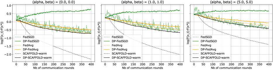
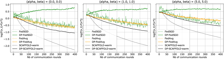
Figure 1: Train Loss On Synthetic Data ($\epsilon=13$). First Row: $K=50$; Second Row: $K=100$.

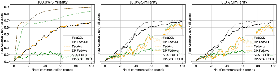
Figure 2: Test Accuracy With $K=50$. First Row: FEMNIST (LogReg), $\epsilon=11.4$; Second Row: MNIST (DNN), $\epsilon=7.2$.

ORGANIZATION OF THE APPENDIX

This appendix is organized as follows. Appendix A summarizes the main notations and provides the detailed DP-FedAvg algorithm for completeness. Appendix B provides details on our privacy analysis. Appendix C gives the full proofs of our utility results for the convex, strongly convex and non-convex cases. Finally, Appendix D provides more details on the experiments of Section 5, as well as additional results.

Appendix A ADDITIONAL INFORMATION

A.1 Table of Notations

Table 2 summarizes the main notations used throughout the paper.

Table 2: Summary of the main notations.

Symbol	Description
$[n]$	set $\{1,2,...,n\}$ for any $n\in\mathbb{N}$
$M$, $i\in[M]$	number and index of users
$T$, $t\in[T]$	number and index of communication rounds
$K$, $k\in[K]$	number and index of local updates (for each user)
$D_{i}$	local dataset held by the $i$-th user, composed of points $d_{1}^{i},\ldots,d^{i}_{R}$
$R$	size of any local dataset $D_{i}$
$D$	joint dataset ($\bigsqcup_{i=1}^{M}D_{i}$)
$f_{i}(x,d)$	loss of the $i$-th user for model $x$ on data record $d$
$F_{i}$	local empirical risk function of the $i$-th user $(\frac{1}{R}\sum_{j=1}^{R}f_{i}(\cdot,d_{j}^{i}))$
$F$	global objective function $(\frac{1}{M}\sum_{i=1}^{M}F_{i})$
$x^{t}\in\mathbb{R}^{d}$	server model after round $t$
$y_{i}^{k}\in\mathbb{R}^{d}$	model of $i$-th user after local update $k$
$c^{t}\in\mathbb{R}^{d}$	server control variate after round $t$
$c_{i}^{t}\in\mathbb{R}^{d}$	control variate of the $i$-th user after round $t$
$l\in(0,1)$	user sampling ratio
$s\in(0,1)$	data sampling ratio
$\epsilon,\delta$	differential privacy parameters
$\sigma_{g}$	standard deviation of Gaussian noise added for privacy
$\mathcal{C}$	gradient clipping threshold
$\nu$	Lipschitz-smoothness constant
$\mu$	strong convexity parameter
$\varsigma^{2}$	variance of stochastic gradients

A.2 DP-FedAvg Algorithm

The code of DP-FedAvg is given in Algorithm 2.

Server Input: initial $x^{0}$

Output: $x^{T}$

1 for $t=1,...,T$ do

2         User subsampling by the server: $C^{t}\subset[M]$ of size $\lfloor lM\rfloor$

3       Server communicates $x^{t-1}$ to users $i\in C^{t}$

4       for user $i\in C^{t}$ do

5             Initialize model: $y_{i}^{0}\leftarrow x^{t}$

6             for $k=1,...,K$ do

7                     Data subsampling by user: $S_{i}^{k}\subset D_{i}$ of size $\lfloor sR\rfloor$

8                   for sample $j\in S_{i}^{k}$ do

9                         Compute gradient: $g_{ij}\leftarrow\nabla f_{i}(y_{i}^{k-1},d^{i}_{j})$

10                           Clip gradient: $\tilde{g}_{ij}\leftarrow g_{ij}/\max\big{(}1,||g_{ij}||_{2}/\mathcal{C}\big{)}$

11                    Add DP noise to local gradients: $\tilde{H}_{i}^{k}\leftarrow\frac{1}{sR}\sum_{j\in S_{i}^{k}}\tilde{g}_{ij}+\frac{2\mathcal{C}}{sR}\mathcal{N}(0,\sigma^{2}_{g})$

12                   $y_{i}^{k}\leftarrow y_{i}^{k-1}-\eta_{l}\tilde{H}_{i}^{k}$

13            $\Delta y_{i}^{t}\leftarrow y_{i}^{K}-x^{t-1}$

14             User $i$ communicates to server: $\Delta y_{i}^{t}$

15      Server aggregates: $\Delta x^{t}\leftarrow\frac{1}{lM}\sum_{i\in C^{t}}\Delta y_{i}^{t}$ 

16       $x^{t}\leftarrow x^{t-1}+\eta_{g}\Delta x^{t}$

Algorithm 2 DP-FedAvg$(T,K,l,s,\sigma_{g},\mathcal{C})$

Appendix B DETAILS ON PRIVACY ANALYSIS

In this section, we provide the proof of our privacy results. We start by recalling standard differential privacy results on composition and amplification by subsampling in Section B.1. Section B.2 reviews recent results in Rényi Differential Privacy (RDP) which allow to obtain tighter privacy bounds. We then formally state and prove Claim 4.1 in Section B.3. Finally, we provide the proof of our main result (Theorem 4.1) in Section B.4.

B.1 Reminders on Differential Privacy

In the following, we denote by $D\in\mathcal{X}^{n}$ to a dataset of size $n$. Two datasets $D,D^{\prime}\in\mathcal{X}^{n}$ are said to be neighboring (denoted by $||D-D^{\prime}||\leq 1$) if they differ by at most one element.

Composition.

Let $M_{1}(\cdot;A_{1}),...,M_{T}(\cdot;A_{T})$ be a sequence of $T$ adaptive DP mechanisms where $A_{t}$ stands for the auxiliary input to the $t$-th mechanism, which may depend on the outputs of previous mechanisms $(M_{t^{\prime}})_{t^{\prime}<t}$. The ability to choose the sequences of mechanisms adaptively is crucial for the design of iterative machine learning algorithms. DP allows to keep track of the privacy guarantees when such a sequence of private mechanisms is run on the same dataset $D$. Simple composition (Dwork et al., 2010, Theorem III.1.) states that the privacy parameters grow linearly with $T$. Dwork et al. (2010) provide a strong composition result where the $\epsilon$ parameter grows sublinearly with $T$. This result is recalled in Lemma B.1.

Lemma B.1 (Strong adaptive composition, Dwork et al., 2010).

Let $M_{1},...,M_{T}$ be $T$ adaptive $(\epsilon,\delta)$-DP mechanisms. Then, for any $\delta^{\prime}>0$, the mechanism $M=(M_{1},...,M_{T})$ is $(\overline{\epsilon},\overline{\delta})$-DP where:

$$\overline{\epsilon}=\epsilon\sqrt{2T\log(1/\delta^{\prime})}+T\epsilon(e^{\epsilon}-1)\text{ and }\overline{\delta}=T\delta+\delta^{\prime}.$$

Remark. When stating theoretical results, $\overline{\epsilon}$ is typically approximated by $\mathcal{O}(\epsilon\sqrt{T\log(1/\delta^{\prime})})$ when $\epsilon<<1$.

Privacy amplification by subsampling.

A key result in DP is that applying a private algorithm on a random subsample of the dataset amplifies privacy guarantees (Kasiviswanathan et al., 2011). In this work, we are interested in subsampling without replacement.

Definition B.1 (Subsampling without replacement).

The subsampling procedure $\text{Samp}_{n,m}:\mathcal{X}^{n}\rightarrow\mathcal{X}^{m}$ (where $m\in\mathbb{N}$, with $m\leq n$) takes $D$ as input and chooses uniformly among its elements a subset $\underline{D}$ of $m$ elements. We may also denote $\text{Samp}_{n,m}$ as $\text{Samp}_{q}$ where $q=m/n$ in the rest of the paper.

Lemma B.2 quantifies the associated privacy amplification effect.

Lemma B.2 (Amplification by subsampling, Kasiviswanathan et al., 2011).

Let $M^{\prime}:\mathcal{X}^{m}\rightarrow\mathcal{Y}$ be a $(\epsilon,\delta)$-DP mechanism w.r.t. a given dataset $\underline{D}\in\mathcal{X}^{m}$. Then, mechanism $M:\mathcal{X}^{n}\rightarrow\mathcal{Y}$ defined as $M:=M^{\prime}\circ\text{Samp}_{n,m}$ is $(\epsilon^{\prime},\delta^{\prime})$-DP w.r.t. to any dataset $D\in\mathcal{X}^{n}$ such that $\underline{D}=\text{Samp}_{n,m}(D)$, where:

$\epsilon^{\prime}=\log(1+q(e^{\epsilon}-1))$, $\delta^{\prime}=q\delta$, $q=m/n$.

Remark. In theoretical results, $\epsilon^{\prime}$ is often approximated by $\mathcal{O}(q\epsilon)$ when $\epsilon<<1$.

B.2 Rényi Differential Privacy

Abadi et al. (2016) demonstrated in practice that the privacy bounds provided by standard $(\epsilon,\delta)$-DP theory (see Section B.1) often overestimate the actual privacy loss. In order to better express inequalities on the tails of the output distributions of private algorithms, we introduce the privacy loss random variable (Dwork and Roth, 2014; Abadi et al., 2016; Wang et al., 2020). Given a random mechanism $M$, let $M(D)$ and $M(D^{\prime})$ be the distributions of the output when $M$ is run on $D$ and $D^{\prime}$ respectively. The privacy loss $L^{M}_{D,D^{\prime}}$ is defined as:

$$L^{M}_{D,D^{\prime}}(\theta):=\log\bigg{(}\displaystyle\frac{M(D)(\theta)}{M(D^{\prime})(\theta)}\bigg{)}\quad\text{where }\theta\sim M(D).$$ (2)

The interpretation of this quantity is easy to understand: $(\epsilon,\delta)$-DP ensures that the absolute value of the privacy loss is bounded by $\epsilon$ with probability at least $(1-\delta)$ for all pairs of neighboring datasets $D$ and $D^{\prime}$ (Dwork and Roth, 2014, Lemma 3.17).

We will reason on the Cumulant Generating Function (CGF) of the privacy loss, denoted $K_{M}$, rather than on the privacy loss $L^{M}$ itself. This CGF is expressed as follows for any $\lambda>0$:

$$K_{M}(D,D^{\prime},\lambda):=\mathbb{E}_{\theta\sim M(D)}\big{[}e^{\lambda L^{M}_{D,D^{\prime}}(\theta)}\big{]}=\mathbb{E}_{\theta\sim M(D)}\bigg{[}\bigg{(}\displaystyle\frac{M(D)(\theta)}{M(D^{\prime})(\theta)}\bigg{)}^{\lambda}\bigg{]},$$

which is also equivalent to:

$$K_{M}(D,D^{\prime},\lambda)=\mathbb{E}_{\theta\sim M(D^{\prime})}\bigg{[}\bigg{(}\displaystyle\frac{M(D)(\theta)}{M(D^{\prime})(\theta)}\bigg{)}^{\lambda+1}\bigg{]}.$$ (3)

By the property of the moment generating function, $K_{M}(D,D^{\prime},\cdot)$ fully determines the distribution of the privacy loss random variable $L^{M}_{D,D^{\prime}}$. We also define $K_{M}(\lambda):=\sup_{||D-D^{\prime}||\leq 1}K_{M}(D,D^{\prime},\lambda)$, which is the upper bound on the CGF for any pair of neighboring datasets.

We can now introduce Rényi Differential Privacy (RDP), which generalizes DP using the Rényi divergence $D_{\alpha}$.

Definition B.2 (Rényi Differential Privacy, Mironov, 2017).

For any $\alpha\in(1,\infty)$ and any $\epsilon>0$, a mechanism $M:\mathcal{X}^{n}\rightarrow\mathcal{Y}$ is said to be $(\alpha,\epsilon)$-RDP, if for all neighboring datasets $D$ and $D^{\prime}$,

$$D_{\alpha}(M(D)||M(D^{\prime})):=\displaystyle\frac{1}{\alpha-1}\log\mathbb{E}_{\theta\sim M(D^{\prime})}\bigg{[}\bigg{(}\displaystyle\frac{M(D)(\theta)}{M(D^{\prime})(\theta)}\bigg{)}^{\alpha}\bigg{]}\leq\epsilon.$$ (4)

Given a mechanism $M$ and a RDP parameter $\alpha$, we can thus determine from Definition B.2 the lowest value of the $\epsilon$-RDP bound, denoted $\epsilon_{M}(\alpha)$, such that $M$ is $(\alpha,\epsilon_{M}(\alpha))$-RDP. Indeed, $\epsilon_{M}(\alpha)$ is such that:

$$\epsilon_{M}(\alpha)=\inf_{\epsilon\in\varepsilon(M)}\epsilon\quad\text{where}\quad\varepsilon(M):=\{\epsilon>0:\sup_{||D-D^{\prime}||\leq 1}D_{\alpha}(M(D)||M(D^{\prime}))\leq\epsilon\}.$$

The obvious similarity between Eq. (3) and Eq. (4) shows the link between the CGF and the notion of RDP. Indeed, for any $\alpha\in(1,\infty)$, it is easy to see that $(\alpha-1)\epsilon_{M}(\alpha)$ is equal to $K_{M}(\lambda)$ where $\lambda+1=\alpha$ (restated in Lemma B.3).

Lemma B.3 (Equivalence RDP-CGF).

Any mechanism $M$ is $(\lambda+1,K_{M}(\lambda)/\lambda)$-RDP for all $\lambda>0$.

We now recall how we can convert RDP guarantees into standard DP guarantees.

Lemma B.4 (RDP to DP conversion, Mironov, 2017).

If $M$ is $(\epsilon,\alpha)$-RDP, then $M$ is $(\epsilon+\log(1/\delta)/(\alpha-1),\delta)$-DP for any $0<\delta<1$.

Given Lemma B.4 and Lemma B.3, it is possible to find the smallest $\epsilon$ from some fixed parameter $\delta$ or the smallest $\delta$ from some fixed parameter $\epsilon$ so as to achieve $(\epsilon,\delta)$-DP:

$$\epsilon(\delta) =\min_{\lambda>0}\displaystyle\frac{\log(1/\delta)+K_{M}(\lambda)}{\lambda},$$ (5)

$$\delta(\epsilon) =\min_{\lambda>0}e^{K_{M}(\lambda)-\lambda\epsilon}.$$ (6)

Moreover, $\lambda\rightarrow K_{M}(\lambda)/\lambda$ is monotonous (Van Erven and Harremos, 2014, Theorem 3) and $\lambda\rightarrow K_{M}(\lambda)$ is convex (Van Erven and Harremos, 2014, Theorem 11). This last property enables to bound $K_{M}$ by a linear interpolation between the values of $K_{M}$ evaluated at integers, as stated below:

$$\forall\lambda>0,K_{M}(\lambda)\leq(1-\lambda+\lfloor\lambda\rfloor)K_{M}(\lfloor\lambda\rfloor)+(\lambda-\lfloor\lambda\rfloor)K_{M}(\lceil\lambda\rceil).$$ (7)

Therefore, Problem (5) is quasi-convex and Problem (6) is log-convex, and both can be solved if we know the expression of $K_{M}(\lambda)$ for any $\lambda>0$.

We provide below other useful results from RDP theory, which we will use in our privacy analysis.

Lemma B.5 (RDP Composition, Mironov, 2017).

Let $\alpha\in(1,\infty)$. Let $M_{1}$ and $M_{2}$ be two mechanisms such that $M_{1}$ is $(\alpha,\epsilon_{1})$-RDP and $M_{2}$, which takes the output of $M_{1}$ as auxiliary input, is $(\alpha,\epsilon_{2})$-RDP. Then the composed mechanism $M_{2}\circ M_{1}$ is $(\alpha,\epsilon_{1}+\epsilon_{2})$-RDP.

Lemma B.6 (RDP Gaussian mechanism, Mironov, 2017).

If $f:\mathcal{X}^{n}\rightarrow\mathbb{R}^{d}$ has $\ell_{2}$-sensitivity 1, then the Gaussian mechanism $G_{f}(\cdot):=f(\cdot)+\mathcal{N}(0,\sigma_{g}^{2}\text{I}_{d})$ is $(\alpha,\alpha/2\sigma_{g}^{2})$-RDP for any $\alpha>1$.

Lemma B.7 (RDP for subsampled Gaussian mechanism, Wang et al., 2020).

Let $\alpha\in\mathbb{N}$ with $\alpha\geq 2$ and $0<q<1$ be a subsampling ratio. Suppose $f:\mathcal{X}^{n}\rightarrow\mathbb{R}^{d}$ has $\ell_{2}$-sensitivity equal to 1. Let $G^{\prime}_{f}(\cdot):=G_{f}\circ\text{Samp}_{q}(\cdot)$ be a subsampled Gaussian mechanism. Then $G^{\prime}_{f}$ is $(\alpha,\epsilon^{\prime}(\alpha,\sigma_{g}^{2}))$-RDP where

$$\epsilon^{\prime}(\alpha,\sigma_{g}^{2})\leq\displaystyle\frac{1}{\alpha-1}\log\bigg{(}1+2q^{2}\binom{\alpha}{2}\min\{2(e^{1/\sigma_{g}^{2}}-1),e^{1/\sigma_{g}^{2}}\}+\displaystyle\sum_{j=3}^{\alpha}2q^{j}\binom{\alpha}{j}e^{j(j-1)/2\sigma_{g}^{2}}\bigg{)}.$$

Remark. By considering $q=o(1)$, the dominant term in the upper bound of $\epsilon^{\prime}(\alpha,\sigma_{g}^{2})$ comes from the term of the sum of the order of $q^{2}$. In particular, when $\sigma_{g}^{2}$ is large (i.e. high privacy regime), the term $\min\{2(e^{1/\sigma_{g}^{2}}-1),e^{1/\sigma_{g}^{2}}\}$ simplifies to $2(e^{1/\sigma_{g}^{2}}-1)\leq 4/\sigma_{g}^{2}$. This thus simplifies the whole upper bound to $\mathcal{O}(\alpha q^{2}/\sigma_{g}^{2})$.

B.3 Proof of Claim 4.1

We restate below a more formal version of Claim 4.1 along with its proof. For any $t\in[T]$, we define subversions of algorithms DP-SCAFFOLD (Alg. 1) and DP-FedAvg (Alg. 2), which stop at round $t$ and reveal an output, either to the server or to a third party:

• To the server. We assume that the sampling of users $C^{t}$ is known by the server. Formally, we define $\mathcal{A}_{\texttt{DP-SCAFFOLD}}^{t}$, which outputs (reveals) $\{y_{i}^{t},c_{i}^{t}\}_{i\in C^{t}}$, and $\mathcal{A}_{\texttt{DP-FedAvg}}^{t}$, which outputs $\{y_{i}^{t}\}_{i\in C^{t}}$ (those quantities being private w.r.t. $\{D_{i}\}_{i\in C^{t}}$).

• To a third party. We define $\mathcal{\tilde{A}}_{\texttt{DP-SCAFFOLD}}^{t}$, which outputs $(x^{t},c^{t})$ and $\mathcal{\tilde{A}}_{\texttt{DP-FedAvg}}^{t}$, which outputs $x^{t}$ (those quantities being private w.r.t. $D$).

In both privacy models, DP-SCAFFOLD and DP-FedAvg can be seen as $T$ adaptive compositions of these sub-algorithms.

Claim B.1 (Formal version of Claim 4.1).

For any $t\in[T]$, the following holds:

• $\mathcal{A}_{\texttt{DP-SCAFFOLD}}^{t}$ and $\mathcal{A}_{\texttt{DP-FedAvg}}^{t}$ have the same level of privacy (towards the server),

• $\mathcal{\tilde{A}}_{\texttt{DP-SCAFFOLD}}^{t}$ and $\mathcal{\tilde{A}}_{\texttt{DP-FedAvg}}^{t}$ have the same level of privacy (towards a third party).

Proof.

We prove the claim by reasoning by induction on the number of communication rounds $t$. We only give the proof for the first statement (including the DP-SCAFFOLD-warm version). The second one can be proved in a similar manner.

First, consider $t=1$. For any $i\in C^{t}$, control variates $c_{i}^{0}$ are either all set to 0 (DP-SCAFFOLD), or $c_{i}^{0}$ are at least as private as $y_{i}^{1}$ (DP-SCAFFOLD-warm). The level of privacy for $\mathcal{A}_{\texttt{DP-SCAFFOLD}}^{1}$ is thus fully determined by the level of privacy of $\{y_{i}^{1}\}_{i\in C^{t}}$, which is the same as $\mathcal{A}_{\texttt{DP-FedAvg}}^{1}$. Therefore the claim is true for $t=1$.

Then, let $t\in[T]$ and suppose that the claim is verified for all $t^{\prime}<t$. Let $i\in C^{t}$ and first consider $\mathcal{A}_{\texttt{DP-SCAFFOLD}}^{t}$. The update of the $i$-th user model (see Eq. 1) at round $t$ shows that an additional information leakage may come from the correction $(c^{t-1}-c_{i}^{t-1})$, or more precisely from $c_{i}^{t-1}$ since $c^{t-1}$ is known by the server. By assumption of induction, $c_{i}^{t-1}$ is also known by the server. Therefore, using the post-processing property of DP, the $y_{i}^{t}$ as updated in DP-SCAFFOLD is as private w.r.t. $D_{i}$ as the $y_{i}^{t}$ as updated in DP-FedAvg. Besides this, the update of the $i$-th control variate fully depends on the local updates of $y_{i}^{t}$ through the average of the DP-noised stochastic gradients calculated over the local iterations. Therefore, considering all the contributions from $C^{t}$, $\mathcal{A}_{\texttt{DP-FedAvg}}^{t}$ and $\mathcal{A}_{\texttt{DP-SCAFFOLD}}^{t}$ have the same level of privacy. ∎

B.4 Proof of Theorem 4.1

Preliminaries.

Lemma B.7 only gives an upper bound of the RDP privacy for a subsampled Gaussian mechanism when $\alpha\in\mathbb{N}$ with $\alpha\geq 2$. However we will need to optimize our privacy bound w.r.t. $\alpha\in\mathbb{R}$ with $\alpha>1$. We thus use Lemma B.3 and the convexity of the CGF (see Eq. 7) to generalize this upper bound to the following result.

Let $\alpha\in\mathbb{R}$ with $\alpha>1$. Under the same assumptions as in Lemma B.7, $G^{\prime}_{f}$ is $(\alpha,\epsilon^{\prime\prime}(\alpha,\sigma_{g}^{2}))$-RDP with

$$\epsilon^{\prime\prime}(\alpha,\sigma_{g}^{2})\leq(1-\alpha+\lfloor\alpha\rfloor)\frac{\lfloor\alpha\rfloor-1}{\alpha-1}\epsilon^{\prime}(\lfloor\alpha\rfloor,\sigma_{g}^{2})+(\alpha-\lfloor\alpha\rfloor)\frac{\lceil\alpha\rceil-1}{\alpha-1}\epsilon^{\prime}(\lceil\alpha\rceil,\sigma_{g}^{2}),$$ (8)

where $\epsilon^{\prime}(\cdot,\sigma_{g}^{2})$ admits the upper bound given in Lemma B.7.

Details of the proof.

Our privacy analysis assumes that the query function has sensitivity 1, since the calibration of the Gaussian noise is locally adjusted in our algorithms with the constant $S=2\mathcal{C}/sR$ (see Section 3.2). We simply denote by $G$ the Gaussian mechanism with variance $\sigma_{g}^{2}$, which is $(\alpha,\alpha/2\sigma_{g}^{2})$-RDP (Lemma B.6). Below, we first prove privacy guarantees towards a third party observing only the final result, and then deduce the guarantees towards the honest-but-curious server.

Step 1: data subsampling.

Let $t\in[T]$ be an arbitrary round. We first provide an upper bound $\epsilon_{a}$ for the privacy loss after the aggregation by the server of the $lM$ individual contributions (line 1 in Alg. 1), thanks to the local addition of noise.

Let $i\in C^{t}$, $\alpha>1$. We denote by $\epsilon_{i}(\alpha)$ the $\alpha$-RDP budget (w.r.t. $D_{i}$) used to “hide” the individual contribution of the $i$-th user from the server. This contribution is the result of the composition of $K$ adaptative $s$-subsampled mechanisms $G$:

• We first obtain an upper RDP bound for the $s$-subsampled mechanism with Lemma B.7. Suppose first $\alpha\in\mathbb{N}$ and $\alpha\geq 2$, which is the case covered by Lemma B.7. Under Assumption 1-(i) and Assumption 1-(iii), the resulting mechanism is $(\alpha,\mathcal{O}(s^{2}\alpha/\sigma_{g}^{2}))$-RDP. To extend this result to $\alpha>1$, we use the result provided in (8): by factoring by $s^{2}/\sigma_{g}^{2}$ in the upper bound of $\epsilon^{\prime\prime}(\alpha,\sigma_{g}^{2})$, and bounding the rest of the inequality (a convex combination between $\lfloor\alpha\rfloor(\lfloor\alpha\rfloor-1)/(\alpha-1)$ and $\lceil\alpha\rceil(\lceil\alpha\rceil-1)/(\alpha-1)$) by $\alpha+1$, we also obtain that this mechanism is $(\alpha,\mathcal{O}(s^{2}(\alpha+1)/\sigma_{g}^{2}))$-RDP.

• We then use the result of Lemma B.5 for the RDP composition rule over the $K$ local iterations, which gives that $\epsilon_{i}(\alpha)\leq\mathcal{O}(Ks^{2}(\alpha+1)/\sigma_{g}^{2})$.

We now consider the aggregation step. Taking into account all the contributions of the users from $C^{t}$, we get a Gaussian noise of variance $S^{2}\sigma_{a}^{2}$ where $\sigma_{a}^{2}=\frac{1}{lM}\sigma_{g}^{2}$. Note that the sensitivity of the aggregation (w.r.t. the joint dataset $D$) is $lM$ times smaller than when considering an individual contribution. Therefore, with the previous approximation, the aggregated contributions satisfy $(\alpha,\mathcal{O}(Ks^{2}(\alpha+1)/lM\sigma_{g}^{2}))$-RDP w.r.t. $D$.

After converting this result into a DP bound (Lemma B.4), we get that for any $0<\delta^{\prime}<1$, the aggregation at line 1 in Alg. 1 is $(\epsilon_{a}(\alpha,\delta^{\prime}),\delta^{\prime})$-DP w.r.t. $D$ where $\epsilon_{a}(\alpha,\delta^{\prime})=\mathcal{O}\big{(}\frac{Ks^{2}(\alpha+1)}{lM\sigma_{g}^{2}}+\frac{\log(1/\delta^{\prime})}{\alpha-1}\big{)}$.

Without approximation: we would obtain at this step an exact upper bound $\epsilon_{a}(\alpha,\delta^{\prime})=K\epsilon^{\prime\prime}(\alpha,lM\sigma_{g}^{2})+\frac{\log(1/\delta^{\prime})}{\alpha-1}$.

Step 2: user subsampling.

In order to get explicit bounds, we then use classical DP tools to estimate an upper DP bound after $T$ rounds taking into account the amplification by subsampling from the set of users. Remark that these tools are however sub-optimal for practical implementations (Abadi et al., 2016, Section 5.1.).

• Using Lemma B.2, the subsampling of users enables a gain of privacy of the order of $l$, which gives $\big{(}\mathcal{O}(l\epsilon_{a}(\alpha,\delta^{\prime})),l\delta^{\prime}\big{)}$-DP.

• Using Lemma B.1, we compose this mechanism over $T$ iterations, which under Assumption 1-(ii) gives for any $\delta^{\prime\prime}>0$, $\big{(}\mathcal{O}(\sqrt{T\log(1/\delta^{\prime\prime})}l\epsilon_{a}(\alpha,\delta^{\prime})),Tl\delta^{\prime}+\delta^{\prime\prime}\big{)}$-DP.

Without approximation: the mechanism is $\big{(}\epsilon^{*}(\alpha,\delta^{\prime})\sqrt{2T\log(1/\delta^{\prime\prime})}+T\epsilon^{*}(\alpha,\delta^{\prime})(e^{\epsilon^{*}(\alpha,\delta^{\prime})}-1),Tl\delta^{\prime}+\delta^{\prime\prime}\big{)}$ where $\epsilon^{*}(\alpha,\delta^{\prime})=\log(1+l(e^{\epsilon_{a}(\alpha,\delta^{\prime})}-1))$.

Step 3: setting parameters.

We denote $\epsilon_{T}(\alpha,\delta^{\prime},\delta^{\prime\prime})=l\sqrt{T\log(1/\delta^{\prime\prime})}\big{(}\frac{Ks^{2}(\alpha+1)}{lM\sigma_{g}^{2}}+\frac{\log(1/\delta^{\prime})}{\alpha-1}\big{)}$. Given what is stated above, the final output of the algorithm is $(\mathcal{O}(\epsilon_{T}),Tl\delta^{\prime}+\delta^{\prime\prime})$-DP.

Considering our final privacy budget $\delta$, we arbitrarily fix $\delta^{\prime}:=\delta/2Tl$ and $\delta^{\prime\prime}:=\delta/2$. We now aim to find an expression of $\sigma_{g}$ such that the privacy bound is minimized. By considering the approximated bound, this gives the following minimization problem:

$$\min_{\alpha>1}\epsilon_{T}(\alpha):=l\sqrt{T\log(2/\delta)}\bigg{(}\frac{Ks^{2}(\alpha+1)}{lM\sigma_{g}^{2}}+\frac{\log(2Tl/\delta)}{\alpha-1}\bigg{)}.$$

Using DP rather than RDP enables to solve this minimization problem pretty easily since only the second factor in $\epsilon_{T}(\alpha)$ depends on $\alpha$, that is:

$$\min_{\alpha>1}\tilde{\epsilon_{T}}(\alpha):=\frac{Ks^{2}(\alpha+1)}{lM\sigma_{g}^{2}}+\frac{\log(2Tl/\delta)}{\alpha-1}.$$

By omitting constants, we obtain the expression for the minimum value of $\epsilon_{T}(\alpha)$:

$$\tilde{\epsilon}=l\sqrt{T\log(2/\delta)}\bigg{(}\frac{s\sqrt{K\log(2Tl/\delta)}}{\sigma_{g}\sqrt{lM}}+\frac{Ks^{2}}{lM\sigma_{g}^{2}}\bigg{)}.$$

Under Assumption 1-(iii), we can bound the second term by the first one, which gives:

$$\tilde{\epsilon}=\mathcal{O}\bigg{(}\frac{s\sqrt{lTK\log(2/\delta)\log(2Tl/\delta)}}{\sigma_{g}\sqrt{M}}\bigg{)}.$$

We then invert the formula of this upper bound of $\tilde{\epsilon}$ to express $\sigma_{g}$ as a function of a given privacy budget $\epsilon$:

$$\sigma_{g}=\Omega\big{(}s\sqrt{lTK\log(2Tl/\delta)\log(2/\delta)}/\epsilon\sqrt{M}\big{)},$$

which proves that the algorithm is $(\mathcal{O}(\epsilon),\delta)$-DP towards a third party observing its final output.

Without approximation: the minimization problem is much more complex and has to be solved numerically

$$\min_{\alpha>1,\delta^{\prime}>0,\delta^{\prime\prime}>0}\epsilon^{*}(\alpha,\delta^{\prime})\sqrt{2T\log(1/\delta^{\prime\prime})}+T\epsilon^{*}(\alpha,\delta^{\prime})(e^{\epsilon^{*}(\alpha,\delta^{\prime})}-1)\quad\text{s.t. }\delta=Tl\delta^{\prime}+\delta^{\prime\prime},$$

or:

$$\min_{\alpha>1,x\in(0,1)}\epsilon^{*}(\alpha,x\delta/Tl)\sqrt{2T\log(1/(1-x)\delta)}+T\epsilon^{*}(\alpha,x\delta/Tl)(e^{\epsilon^{*}(\alpha,x\delta/Tl)}-1).$$

Extension to privacy towards the server.

The crucial difference with the third party case is that the server observes individual contributions and knows which users are subsampled at each step. Removing the privacy amplification effect of the $l$-subsampling of users and the aggregation step, the minimization problem becomes

$$\min_{\alpha>1}\epsilon_{T}(\alpha):=\sqrt{T\log(2/\delta)}\bigg{(}\frac{Ks^{2}\alpha}{\sigma_{g}^{2}}+\frac{\log(2T/\delta)}{\alpha-1}\bigg{)},$$

where the minimizing value can be approximated by:

$$\tilde{\epsilon}=\sqrt{T\log(2/\delta)}\bigg{(}\frac{s\sqrt{K\log(2T/\delta)}}{\sigma_{g}}+\frac{Ks^{2}}{\sigma_{g}^{2}}\bigg{)}.$$

Under Assumption 1-(iii), we can bound the second term by the first one:

$$\tilde{\epsilon}=\mathcal{O}\bigg{(}\frac{s\sqrt{TK\log(2/\delta)\log(2T/\delta)}}{\sigma_{g}}\bigg{)},$$

which proves that we obtain $(\mathcal{O}(\epsilon_{s}),\delta_{s})$-DP towards the server where $\epsilon_{s}=\mathcal{\epsilon}\sqrt{\frac{M}{l}}$ and $\delta_{s}=\frac{\delta}{2}(\frac{1}{l}+1)$.

Finer results for amplification by subsampling.

To establish privacy towards a third party, it is actually possible to combine the subsampling ratios (user and data) to determine a bound upon the subsampling of data directly from $D$ and thus to quantify a more precise gain in privacy (Girgis et al., 2021b). The difficulty in this setup is that this combined subsampling is not uniform overall, which requires extending the proof of Lemma B.2 as done by Girgis et al. (2021b) in the case of classical differential privacy.

Implementation.

In practice, we determine a RDP upper bound at Step 2, by using the theorem proved by Wang et al. (2020) (which is not restricted to Gaussian mechanisms) with the exact RDP bound obtained at Step 1 and sampling parameter $l$. This result being accurate only for $\alpha\in\mathbb{N}\setminus\{0,1\}$, we obtain an natural extension of the bound for any $\alpha>1$ with Eq (7). Then, we invoke Lemma B.5 to obtain the final RDP bound after $T$ communication rounds, for any $\alpha>1$. Under fixed privacy parameter $\delta$ (chosen as $1/MR$ in our experiments), we finally obtain the minimal value for $\epsilon$ w.r.t. $\alpha\in(1,\infty)$, which is determined by Eq (5). The last step is done by using a fine grid search over parameter $\alpha$.

Appendix C PROOF OF UTILITY

In this section, we provide the proof of our utility results. We first establish in Section C.1 some preliminary results about the impact of DP noise over stochastic gradients. In Section C.2, we provide the complete version of our utility result for DP-SCAFFOLD-warm (Theorem C.1), from which Theorem 4.2 is an immediate corollary. We prove this theorem for convex local loss functions in Section C.3 and non-convex loss functions in Section C.4. We finally state in Section C.5 our complete result for DP-FedAvg (Theorem C.2).

For any $\mathcal{C},\sigma_{g}>0$, we define $\Sigma_{g}(\mathcal{C}):=2\mathcal{C}\sqrt{2d}\sigma_{g}/sR$. We recall that we assume that $F$ is bounded from below by $F^{*}=F(x^{*})$, for an $x^{*}\in\mathbb{R}^{d}$.

C.1 Preliminaries

Properties of DP-noised stochastic gradients.

Let $i\in[M]$, $x\in\mathbb{R}^{d}$, $S_{i}\subset D_{i}$ and $\mathcal{C},\sigma_{g}>0$. Suppose Assumptions 2 and 3.3 are verified (the last assumption ensures that the clipping on per-example local gradients with threshold $\mathcal{C}$ is not effective).

We recall below the expression of $\tilde{H}_{i}(x)$ from Section 3.3, which is the noised version of the local gradient $H_{i}(x)$ of the $i$-th user over $S_{i}$ evaluated at $x$ (omitting index $k$):

$$\tilde{H}_{i}(x):=H_{i}(x)+\frac{2\mathcal{C}}{sR}\mathcal{N}(0,\sigma^{2}_{g}),\quad\text{where}\quad H_{i}(x):=\frac{1}{sR}\sum_{d_{j}^{i}\in S_{i}}\nabla f_{i}(x,d^{i}_{j}).$$

We recall that the $\ell_{2}$-sensitivity of $H_{i}(x)$ w.r.t. $S_{i}$ is upper bounded by $2\mathcal{C}/sR$, which explains the scaling of the Gaussian noise in the expression of $\tilde{H}_{i}(x)$. Since the variance of $\mathcal{N}(0,\text{I}_{d})$ is $2d$, the following statement holds directly:

$$\mathbb{E}\big{[}\tilde{H}_{i}(x)\big{]}=H_{i}(x)\text{ and }\mathbb{E}\big{[}||\tilde{H}_{i}(x)-H_{i}(x)||^{2}\big{]}\leq\displaystyle\frac{8\mathcal{C}^{2}d\sigma_{g}^{2}}{s^{2}R^{2}}=\Sigma_{g}(\mathcal{C})^{2}.$$

By combining our utility assumptions with the result stated above, we can deduce the following lemma.

Lemma C.1 (Regularity of DP-noised stochastic gradients).

Under Assumptions 2 and 3, for any iteration $t\in[T],k\in[K]$,

1. $\mathbb{E}\big{[}\tilde{H}_{i}^{k}(y_{i}^{k-1})|y_{i}^{k-1}\big{]}=\nabla F_{i}(y_{i}^{k-1})$,

2. $\mathbb{E}\big{[}||\tilde{H}_{i}^{k}(y_{i}^{k-1})-\nabla F_{i}(y_{i}^{k-1})||^{2}|y_{i}^{k-1}\big{]}\leq\displaystyle\frac{\varsigma^{2}}{sR}+\Sigma_{g}^{2}(\mathcal{C})$.

The proof of Lemma C.1 is easily obtained by conditioning on the two sources of randomness (i.e., mini-batch sampling and Gaussian noise) which are independent, thus the variance is additive. This result can be seen as a degraded version of Assumption 3 due to the local injection DP noise, a fact that we will strongly leverage to derive convergence rates.

We now enumerate several statements that will be used in the utility proof. First, Lemma C.2 enables to control $||\nabla F||^{2}$ using the assumption of smoothness over the local loss functions. Second, Lemma C.3 provides separation inequalities of mean and variance (Karimireddy et al., 2020b, Lemma 4), which enables to state a result on quantities of interest in Corollary C.1.

Lemma C.2 (Nesterov inequality).

Suppose Assumption 2 is verified and assume that for all $i\in[M]$, $F_{i}$ is convex. Then,

$$\forall x\in\mathbb{R}^{d},||\nabla F(x)||^{2}\leq 2\nu(F(x)-F^{*}).$$

Proof.

Let $x\in\mathbb{R}^{d}$.

$$||\nabla F(x)||^{2} =||\nabla F(x)-\nabla F(x^{*})||^{2}=||\frac{1}{M}\sum_{i=1}^{M}\nabla F_{i}(x)-\nabla F_{i}(x^{*})||^{2}$$

$$\leq\frac{1}{M}\sum_{i=1}^{M}||\nabla F_{i}(x)-\nabla F_{i}(x^{*})||^{2}$$ (Jensen inequality)

$$\leq 2\nu(F(x)-F^{*})$$ (Nesterov et al., 2004, Theorem 2.1.5)

∎

Lemma C.3 (Separating mean and variance).

Let $(A_{1},...,A_{n})$ be $n$ random variables in $\mathbb{R}^{d}$ not necessarily independent.
1. Suppose that their mean is $\mathbb{E}[A_{i}]=a_{i}$ and their variance is uniformly bounded, i.e. for all $i\in[n]$, $\mathbb{E}[||A_{i}-a_{i}||^{2}]\leq\sigma^{2}_{A}$. Then,

$$\mathbb{E}\left\|\displaystyle\sum_{i=1}^{n}A_{i}\right\|^{2}\leq\left\|\displaystyle\sum_{i=1}^{n}a_{i}\right\|^{2}+n^{2}\sigma^{2}_{A}.$$

2. Suppose that their conditional mean is $\mathbb{E}[A_{i}|A_{i-1},...A_{1}]=a_{i}$ and their variance is uniformly bounded, i.e. for all $i\in[n]$, $\mathbb{E}[||A_{i}-a_{i}||^{2}]\leq\sigma^{2}_{A}$. Then,

$$\mathbb{E}\left\|\displaystyle\sum_{i=1}^{n}A_{i}\right\|^{2}\leq 2\left\|\displaystyle\sum_{i=1}^{n}a_{i}\right\|^{2}+2n\sigma^{2}_{A}.$$

Corollary C.1.

Let $t\in[T]$. In the following statements, the expectation is taken w.r.t. the randomness from their local data sampling and from the Gaussian DP noise, conditionally to the users’ sampling $C^{t}$ and initial value of variables $y_{i}$, that is $y^{0}=x^{t-1}$ (same for all users). We have:

• $\mathbb{E}\left[\Big{\|}\displaystyle\frac{1}{KlM}\sum_{i\in C^{t}}\sum_{k\in[K]}(\tilde{H}_{i}^{k}(y_{i}^{k-1})-\nabla F_{i}(y_{i}^{k-1}))\Big{\|}^{2}\bigg{|}C^{t},y^{0}\right]{\leq}\displaystyle\frac{\Sigma_{g}^{2}(\mathcal{C})+\varsigma^{2}/sR}{KlM}$,

• $\mathbb{E}\bigg{[}\Big{\|}\displaystyle\frac{1}{lM}\sum_{i\in C^{t}}c_{i}^{t}-\mathbb{E}[c^{t}_{i}]\Big{\|}^{2}|C^{t},y^{0}\bigg{]}\leq\frac{\Sigma_{g}^{2}(\mathcal{C})+\varsigma^{2}/sR}{KlM}$,

• $\mathbb{E}\bigg{[}\Big{\|}c^{t}-\mathbb{E}[c^{t}]\Big{\|}^{2}|y^{0}\bigg{]}\leq\displaystyle\frac{\Sigma_{g}^{2}(\mathcal{C})+\varsigma^{2}/sR}{KlM}$.

Proof.

First inequality. We define a random variable $A$ such as $A:=\frac{1}{KlM}\sum_{i\in C^{t}}\sum_{k\in[K]}A_{i,k}$, with $A_{i,k}:=\tilde{H}_{i}^{k}(y_{i}^{k-1})$.

From Lemma C.1, we have that for all $i\in C^{t},k\in[K]$: $\mathbb{E}[A_{i,k}|y_{i}^{k-1}]=\mathbb{E}[\tilde{H}_{i}^{k}(y_{i}^{k-1})|y_{i}^{k-1}]=\nabla F_{i}(y_{i}^{k-1})$. Furthermore, by Lemma C.1, $\mathbb{E}\left[||\tilde{H}_{i}^{k}(y_{i}^{k-1})-\nabla F_{i}(y_{i}^{k-1})||^{2}|y_{i}^{k-1}\right]\leq\Sigma_{g}^{2}(\mathcal{C})+\varsigma^{2}/sR$.

Furthermore, (a) for $i,j\in C^{t}$, $\sum_{k\in[K]}A_{i,k}-\nabla F_{i}(y_{i}^{k-1})$ and $\sum_{k\in[K]}A_{j,k}-\nabla F_{j}(y_{j}^{k-1})$ are independent conditionally to $y^{0}$; (b) for any $i\in C^{t}$, $(A_{i,k}-\nabla F_{i}(y_{i}^{k-1}))_{k\in[K]}$ is a martingale increment, i.e., $\mathbb{E}[A_{i,k}-\nabla F_{i}(y_{i}^{k-1})|\sigma(\{y_{i}^{k^{\prime}}\}_{k^{\prime}\in[k-1]})]=0$. Consequently:

$$\mathbb{E}\left[\Big{\|}\frac{1}{KlM}\sum_{i\in C^{t}}\sum_{k\in[K]}A_{i,k}-\nabla F_{i}(y_{i}^{k-1})\Big{\|}^{2}\bigg{|}C^{t},y^{0}\right] \overset{(a)}{=}\frac{1}{(KlM)^{2}}\sum_{i\in C^{t}}\mathbb{E}\left[\Big{\|}\sum_{k\in[K]}A_{i,k}-\nabla F_{i}(y_{i}^{k-1})\Big{\|}^{2}\bigg{|}y^{0}\right]$$

$$\overset{(b)}{=}\frac{1}{(KlM)^{2}}\sum_{i\in C^{t}}\sum_{k\in[K]}\mathbb{E}\left[\underbrace{\mathbb{E}\left[\Big{\|}A_{i,k}-\nabla F_{i}(y_{i}^{k-1})\Big{\|}^{2}\bigg{|}\sigma\big{(}\{y_{i}^{k^{\prime}}\}_{k^{\prime}\in[k]}\big{)}\right]}_{\leq\Sigma_{g}^{2}(\mathcal{C})+\varsigma^{2}/sR}\bigg{|}y^{0}\right]$$

$${\leq}\frac{\Sigma_{g}^{2}(\mathcal{C})+\varsigma^{2}/sR}{KlM}.$$

To prove the second equality, we need to “iteratively” expand the squared norm and take the conditional expectation w.r.t. $\sigma\big{(}\{y_{i}^{k^{\prime}}\}_{k^{\prime}\in[k]}\big{)}$ for $k=K,K-1,\ldots,1$ and use the martingale property to obtain that the scalar products are equal to 0.

Second inequality. We recall that for any $i\in C^{t}$, $c_{i}^{t}=\frac{1}{K}\sum_{k=1}^{K}\tilde{H}_{i}^{k}(y_{i}^{k-1})$. Thus $\frac{1}{lM}\sum_{i\in C^{t}}c_{i}^{t}=A$ and we can directly use the results from the first inequality.

Third inequality. We recall that $c^{t}=\frac{1}{M}\sum_{i=1}^{M}c_{i}^{t}$ (even if local control variates are not updated). Therefore, we can use the previous results and take the expectation over $C^{t}$, which gives:

$$\mathbb{E}\bigg{[}\Big{\|}c^{t}-\mathbb{E}[c^{t}]\Big{\|}^{2}|y^{0}\bigg{]}\leq\displaystyle\frac{\varsigma^{2}/sR+\Sigma^{2}_{g}(\mathcal{C})}{KM}\leq\frac{\varsigma^{2}/sR+\Sigma^{2}_{g}(\mathcal{C})}{KlM}.$$

∎

C.2 Theorem of Convergence for DP-SCAFFOLD-warm

Theorem C.1 (Utility rates for DP-SCAFFOLD-warm, $\sigma_{g}$ chosen arbitrarily).

Let $\sigma_{g},\mathcal{C}>0$, $x^{0}\in\mathbb{R}^{d}$. Suppose we run DP-SCAFFOLD-warm$(T,K,l,s,\sigma_{g},\mathcal{C})$ with initial local controls such that $c_{i}^{0}=\frac{1}{K}\sum_{k=1}^{K}\tilde{H}_{i}^{k}(x^{0})$ for any $i\in[M]$. Under Assumptions 2 and 3, we consider the sequence of iterates $(x^{t})_{t\geq 0}$ of the algorithm, starting from $x^{0}$.

1. If $F_{i}$ are $\mu$-strongly convex ($\mu>0$), $\eta_{g}=\sqrt{lM}$, $\bar{\eta}_{l}=\min\big{(}\frac{l^{\frac{2}{3}}}{24\nu K\eta_{g}},\frac{l}{54\mu K\eta_{g}}\big{)}$, and $T\geq\max(\frac{54}{l},\frac{24\nu}{\mu l^{\frac{2}{3}}})$, then there exist weights $\{w_{t}\}_{t\in[T]}$ and local step-sizes $\eta_{l}\leq\bar{\eta}_{l}$ such that the averaged output of DP-SCAFFOLD-warm$(T,K,l,s,\sigma_{g},\mathcal{C})$, defined by $\overline{x}^{T}=\sum_{t\in[T]}w_{t}x^{t}$, has expected excess of loss such that:

   $\mathbb{E}[F(\overline{x}^{T})]-F(x^{*})\leq\mathcal{O}\bigg{(}\displaystyle\frac{\varsigma^{2}/sR+\Sigma^{2}_{g}(\mathcal{C})}{\mu TKlM}+\mu D_{0}^{2}\exp(-\min\big{(}\frac{l}{108},\frac{\mu l^{\frac{2}{3}}}{48\nu}\big{)}T)\bigg{)}$,

2. If $F_{i}$ are convex, $\eta_{g}=\sqrt{lM}$, $\bar{\eta}_{l}=\min\big{(}\frac{l^{\frac{2}{3}}}{24\nu K\eta_{g}},\frac{D_{0}\sqrt{KlM}}{K\eta_{g}\sqrt{T(\varsigma^{2}/sR+\Sigma_{g}(\mathcal{C})^{2})}}\big{)}$ and $T\geq 1$, then there exist weights $\{w_{t}\}_{t\in[T]}$ and local step-sizes $\eta_{l}\leq\bar{\eta}_{l}$ such that the averaged output of DP-SCAFFOLD-warm$(T,K,l,s,\sigma_{g},\mathcal{C})$, defined by $\overline{x}^{T}=\sum_{t\in[T]}w_{t}x^{t}$, has expected excess of loss such that:

   $\mathbb{E}[F(\overline{x}^{T})]-F(x^{*})\leq\mathcal{O}\bigg{(}\displaystyle\frac{\varsigma/\sqrt{sR}+\Sigma_{g}(\mathcal{C})}{\sqrt{TKlM}}D_{0}+\frac{\nu}{l^{\frac{2}{3}}T}D_{0}^{2}\bigg{)}$,

3. If $F_{i}$ are non-convex, $\eta_{g}=\sqrt{lM}$, $\bar{\eta}_{l}=\frac{l^{\frac{2}{3}}}{24\nu K\eta_{g}}$ and $T\geq 1$, then there exist weights $\{w_{t}\}_{t\in[T]}$ and local step-sizes $\eta_{l}\leq\bar{\eta}_{l}$ such that the randomized output of DP-SCAFFOLD-warm$(T,K,l,s,\sigma_{g},\mathcal{C})$, defined by $\{\overline{x}^{T}=x^{t}\text{ with probability }w_{t}\text{ for all }t\}$, has expected squared gradient of the loss such that:

   $\mathbb{E}||\nabla F(\overline{x}^{T})||^{2}\leq\mathcal{O}\bigg{(}\displaystyle\frac{\varsigma/\sqrt{sR}+\Sigma_{g}(\mathcal{C})}{\sqrt{TKlM}}\sqrt{F_{0}}+\frac{\nu}{l^{\frac{2}{3}}T}F_{0}\bigg{)}$,

where $D_{0}=||x^{0}-x^{*}||$ and $F_{0}:=F(x^{0})-F^{*}$.

We recover the result of Theorem 4.2 for DP-SCAFFOLD-warm where $F_{i}$ are convex by setting $\sigma_{g}=\sigma_{g}^{*}$ where $\sigma_{g}^{*}:=s\sqrt{lTK\log(2Tl/\delta)\log(2/\delta)}/\epsilon\sqrt{M}$, which gives $\Sigma_{g}(\mathcal{C})=2\mathcal{C}d\sqrt{2lTK\log(2Tl/\delta)\log(2/\delta)}/\epsilon R\sqrt{M}$ (with numerical constants omitted for the asymptotic bound).

C.3 Proof of Theorem C.1 (Convex case)

In this section, we give a detailed proof of convergence of DP-SCAFFOLD-warm with convex local loss functions. Our analysis is adapted from the proof given by Karimireddy et al. (2020b) without DP noise, but requires original modifications (see below). Throughout this part, we re-use the notations from Section 3.3.

Summary of the main steps.

Let $t\in[T]$ be an arbitrary communication round of the algorithm. We detail below the updates that occur at this round.

• Let $i\in C^{t}$. Starting from $y_{i}^{0}=x^{t-1}$, the random variable $y_{i}$ is updated at local step $k\in[K]$ such that $y_{i}^{k}:=y_{i}^{k-1}-\eta_{l}v_{i,k}^{t}$ where $v_{i,k}^{t}=\tilde{H}_{i}^{k}(y_{i}^{k-1})-c_{i}^{t-1}+c^{t-1}$.

• Then we define the local control variate $\tilde{c}_{i}^{t}$ for this user by:

  $$\tilde{c}_{i}^{t}:=c^{t-1}-c_{i}^{t-1}+\displaystyle\frac{1}{K\eta_{l}}(x^{t-1}-y_{i}^{K})=\frac{1}{K}\sum_{k=1}^{K}\tilde{H}_{i}^{k}(y_{i}^{k-1}).$$

• For any $i\in[M]$, we update the control variate $c_{i}^{t}$ such that:

  • $c_{i}^{t}:=\tilde{c}_{i}^{t}$ if $i\in C^{t}$,

  • $c_{i}^{t}:=c_{i}^{t-1}$ otherwise.

• Finally, the global update is computed as:

  $x^{t}=x^{t-1}+\displaystyle\frac{\eta_{g}}{lM}\sum_{i\in C^{t}}(y_{i}^{K}-x^{t-1})$ and $c^{t}=\displaystyle\frac{1}{M}\big{(}\sum_{i\in C^{t}}c_{i}^{t}+\sum_{i\notin C^{t}}c_{i}^{t-1}\big{)}$.

To keep track of the lag in the update of $c_{i}^{t}$, we introduce $\alpha_{i,k-1}^{t}$ defined for any $i\in[M]$, any $t\in[T]$ and any $k\in[K]$ by:

$$\alpha_{i,k-1}^{t}=\left\{\begin{array}[]{ll}y_{i}^{k-1}&\text{ if }i\in C^{t}\\ \alpha_{i,k-1}^{t-1}&\text{ otherwise}\end{array}\right.$$

with $\alpha_{i,k-1}^{0}=x^{0}$.

We hence have the following property for any $i\in[M]$ and any $t\in[T]$: $c_{i}^{t}=\frac{1}{K}\sum_{k=1}^{K}\tilde{H}_{i}^{k}(\alpha_{i,k-1}^{t})$.

Additional definitions.

• Model gap: $\Delta x^{t}:=x^{t}-x^{t-1}$,

• Global step-size: $\tilde{\eta}:=K\eta_{l}\eta_{g}$ which gives $\Delta x^{t}=-\displaystyle\frac{\tilde{\eta}}{KlM}\sum_{k\in[K],i\in C^{t}}\tilde{H}_{i}^{k}(y_{i}^{k-1})+c^{t-1}-c_{i}^{t-1}$,

• User-drift: $\mathcal{E}_{t}:=\displaystyle\frac{1}{KM}\sum_{k=1}^{K}\sum_{i=1}^{M}\mathbb{E}||y_{i}^{k}-x^{t-1}||^{2}$,

• Control lag: $\mathcal{F}_{t}:=\displaystyle\frac{1}{KM}\sum_{k=1}^{K}\sum_{i=1}^{M}\mathbb{E}||\alpha_{i,k-1}^{t}-x^{t}||^{2}$ with $\mathcal{F}_{0}=0$.

Originality of the proof.

The proof substantially differs form the proof by Karimireddy et al. (2020b) in the convex case. Indeed, Karimireddy et al. (2020b) control a combination of the quadratic distance to the optimum and a control of the deviation between the controls and the gradients at the optimal point $\|c_{i}^{t}-\nabla F_{i}(x^{*})\|.$ Leveraging such a quantity in our proof would result in a worse upper bound on the utility than the one we get, as either the noise added to ensure DP (if $c_{i}^{0}$ is defined w.r.t. a noised gradient) or the heterogeneity (if $c_{i}^{0}=0$) would also appear in the initial condition $\|c_{i}^{t}-\nabla F_{i}(x^{*})\|.$ On the other hand, in our approach, we combine the quadratic distance to the optimum to a control of the lag and user-drift. In some sense this resembles some aspects of the proof in the non-convex regime in (Karimireddy et al., 2020b), in which the excess risk ($F(x^{t})-F^{*}$) is combined with the lag. Nevertheless, our result (in the convex case), strongly leverages the convexity of the function in the proof.

Details of the proof.

The idea of the proof is to find a contraction inequality involving $||x^{t}-x^{*}||^{2}$, $\mathbb{E}[F(x^{t-1})]-F(x^{*})$, $\mathcal{F}_{t}$ and $\varsigma/\sqrt{sR}+\Sigma_{g}(\mathcal{C})$. To do so, we will first bound the variance of the server’s update. Then we will see how the control lag evolves through the communication rounds. We will also bound the user drift. To make the proof more readable, the index $t$ may be omitted on random variables when the only communication round that is considered is the $t$-th one.

Lemma C.4 (Variance of the server’s update).

$\forall\tilde{\eta}\in[0,1/\nu]$

$$\mathbb{E}||x^{t}-x^{t-1}||^{2}\leq 4\tilde{\eta}^{2}\nu^{2}\mathcal{E}_{t}+8\nu^{2}\tilde{\eta}^{2}\mathcal{F}_{t-1}+8\nu\tilde{\eta}^{2}\mathbb{E}\big{(}F(x^{t-1})-F(x^{*})\big{)}+\frac{9\tilde{\eta}^{2}}{KlM}(\varsigma^{2}/sR+\Sigma_{g}^{2}(\mathcal{C})).$$

Proof.

We consider the model gap $\Delta x^{t}=x^{t}-x^{t-1}$.

$$\mathbb{E}||\Delta x^{t}||^{2}=\tilde{\eta}^{2}\mathbb{E}\Big{\|}\underbrace{\bigg{(}\frac{1}{KlM}\sum_{k\in[K],i\in C^{t}}\tilde{H}_{i}(y_{i}^{k-1})\bigg{)}}_{A_{1}}+\underbrace{c^{t-1}}_{A_{2}}-\underbrace{\frac{1}{lM}\sum_{i\in C^{t}}c_{i}^{t-1}}_{A_{3}}\Big{\|}^{2}$$

We combine Lemma C.3-1 on $A_{1},A_{2},A_{3}$ with Corollary C.1 which controls their individual variance (conditionally to the users’ sampling and the local parameters) by $\frac{\varsigma^{2}/sR+\Sigma_{g}^{2}(\mathcal{C})}{KlM}$. We first get rid of the terms related to the variance of the data sampling and the DP noise, before bounding the quantities of interest. It leads to:

$$\mathbb{E}||\Delta x^{t}||^{2} =\tilde{\eta}^{2}\mathbb{E}\left[\mathbb{E}\left[\bigg{\|}\bigg{(}\frac{1}{KlM}\sum_{k\in[K],i\in C^{t}}\tilde{H}_{i}(y_{i}^{k-1})\bigg{)}+c^{t-1}-\frac{1}{lM}\sum_{i\in C^{t}}c_{i}^{t-1}\bigg{\|}^{2}\bigg{|}C^{t},y^{0}\right]\right]$$

$$\leq\tilde{\eta}^{2}\mathbb{E}\left[\Big{\|}\frac{1}{KlM}\sum_{k\in[K],i\in C^{t}}\mathbb{E}[\tilde{H}_{i}(y_{i}^{k-1})|y^{0}]+\mathbb{E}[c^{t-1}|y^{0}]-\mathbb{E}[c_{i}^{t-1}|y^{0}]\Big{\|}^{2}\right]+\frac{9\tilde{\eta}^{2}}{KlM}(\varsigma^{2}/sR+\Sigma_{g}^{2}(\mathcal{C})),$$

where the inequality is given by Lemma C.3-1.

For any $i\in C^{t},k\in[K]$, we have $\mathbb{E}[\tilde{H}_{i}(y_{i}^{k-1})|y^{0}]=\mathbb{E}\left[\mathbb{E}[\tilde{H}_{i}(y_{i}^{k-1})|y_{i}^{k-1}]\big{|}y^{0}\right]=\mathbb{E}\left[\nabla F_{i}(y_{i}^{k-1})|y^{0}\right]=\nabla F_{i}(y_{i}^{k-1})$. Then,

$$\mathbb{E}||\Delta x^{t}||^{2} \leq\tilde{\eta}^{2}\mathbb{E}\left[\frac{1}{KlM}\sum_{k\in[K],i\in C^{t}}\Big{\|}\nabla F_{i}(y_{i}^{k-1})+\mathbb{E}[c^{t-1}|y^{0}]-\mathbb{E}[c_{i}^{t-1}|y^{0}]\Big{\|}^{2}\right]+\frac{9\tilde{\eta}^{2}}{KlM}(\varsigma^{2}/sR+\Sigma_{g}^{2}(\mathcal{C}))\qquad\text{(convexity of $||.||^{2}$)}$$

$$=\tilde{\eta}^{2}\frac{1}{KM}\sum_{k\in[K],i\in[M]}\mathbb{E}\Big{[}\Big{\|}\underbrace{\nabla F_{i}(y_{i}^{k-1})+\mathbb{E}[c^{t-1}|y^{0}]-\mathbb{E}[c_{i}^{t-1}|y^{0}]}_{\begin{subarray}{c}\nabla F_{i}(y_{i}^{k-1})-\nabla F_{i}(x^{t-1})\\ +\mathbb{E}[c^{t-1}|y^{0}]-\nabla F(x^{t-1})\\ -\mathbb{E}[c_{i}^{t-1}|y^{0}]+\nabla F_{i}(x^{t-1})\\ +\nabla F(x^{t-1})\end{subarray}}\Big{\|}^{2}\Big{]}+\frac{9\tilde{\eta}^{2}}{KlM}(\varsigma^{2}/sR+\Sigma_{g}^{2}(\mathcal{C}))\qquad\text{(definition of $C^{t}$)}$$

$$=\tilde{\eta}^{2}\frac{1}{KM}\sum_{k\in[K],i\in[M]}\mathbb{E}\left[\Big{\|}\mathbb{E}\left[\nabla F_{i}(y_{i}^{k-1})-\nabla F_{i}(x^{t-1})+c^{t-1}-\nabla F(x^{t-1})-c_{i}^{t-1}+\nabla F_{i}(x^{t-1})+\nabla F(x^{t-1})\Big{|}y^{0}\right]\Big{\|}^{2}\right]$$

$$+\frac{9\tilde{\eta}^{2}}{KlM}(\varsigma^{2}/sR+\Sigma_{g}^{2}(\mathcal{C}))\qquad\qquad\qquad\text{(all variables are measurable wrt $y^{0}$)}$$

$$\leq\tilde{\eta}^{2}\frac{1}{KM}\sum_{k\in[K],i\in[M]}\mathbb{E}\left[\mathbb{E}\left[\Big{\|}\nabla F_{i}(y_{i}^{k-1})-\nabla F_{i}(x^{t-1})+c^{t-1}-\nabla F(x^{t-1})-c_{i}^{t-1}+\nabla F_{i}(x^{t-1})+\nabla F(x^{t-1})\Big{\|}^{2}\Big{|}y^{0}\right]\right]$$

$$+\frac{9\tilde{\eta}^{2}}{KlM}(\varsigma^{2}/sR+\Sigma_{g}^{2}(\mathcal{C}))\qquad\qquad\qquad\text{(Jensen inequality)}$$

$$\leq\frac{4\tilde{\eta}^{2}}{KM}\sum_{k\in[K],i\in[M]}\mathbb{E}\left[\Big{\|}\nabla F_{i}(y_{i}^{k-1})-\nabla F_{i}(x^{t-1})\Big{\|}^{2}\right]+\frac{8\tilde{\eta}^{2}}{KM}\sum_{k\in[K],i\in[M]}\mathbb{E}\left[\Big{\|}\nabla F_{i}(\alpha_{i,k-1}^{t-1})-\nabla F_{i}(x^{t-1})\Big{\|}^{2}\right]$$

$$+4\tilde{\eta}^{2}\mathbb{E}\Big{\|}\nabla F(x^{t-1})\Big{\|}^{2}+\frac{9\tilde{\eta}^{2}}{KlM}(\varsigma^{2}/sR+\Sigma_{g}^{2}(\mathcal{C})).$$

The last inequality is obtained by definition of $c$ and $c_{i}$ and by applying Jensen inequality. With Lemma C.2, this leads to the result. ∎

Lemma C.5 (Lag in the control variate).

$\forall\alpha\in[1/2,1],\forall\tilde{\eta}\leq\frac{1}{24\nu}l^{\alpha}$,

$$\mathcal{F}_{t}\leq\left(1-\frac{17}{36}l\right)\mathcal{F}_{t-1}+\frac{1}{24\nu}l^{2\alpha-1}\mathbb{E}\big{(}F(x^{t-1})-F(x^{*})\big{)}+\frac{97}{48}l^{2\alpha-1}\mathcal{E}_{t}+\frac{l}{\nu^{2}}\frac{\varsigma^{2}/sR+\Sigma_{g}^{2}(\mathcal{C})}{32KlM}.$$

Proof.

We adapt the original proof made in the non-convex case (Karimireddy et al., 2020b, Lemma 16) and use Lemma C.1 and Lemma C.2. ∎

Lemma C.6 (Bounding the user drift).

$\forall\eta_{g}\geq 1,\forall\eta_{l}\leq 1/24\nu K\eta_{g}$,

$$\frac{9}{2}\nu^{2}\tilde{\eta}\mathcal{E}_{t}\leq\frac{9}{2}\nu^{3}\tilde{\eta}^{2}\mathcal{F}_{t-1}+\frac{9}{40}\frac{\tilde{\eta}\nu}{\eta_{g}^{2}}\mathbb{E}\big{(}F(x^{t-1})-F(x^{*})\big{)}+\frac{27}{40}\frac{\tilde{\eta}^{2}\nu}{K\eta_{g}^{2}}\big{(}\varsigma^{2}/sR+\Sigma_{g}^{2}(\mathcal{C})\big{)}.$$

Proof.

We once again adapt the original proof made in the non-convex case (Karimireddy et al., 2020b, Lemma 17), use Lemma C.2 and multiply on each side of the inequality by $\frac{9}{2}\nu^{2}\tilde{\eta}$. ∎

Lemma C.7 (Progress made at each round).

$\forall\eta_{g}\geq 1,\forall\eta_{l}\leq\min\big{(}\frac{1}{24K\eta_{g}\nu}l^{2/3},\frac{l}{54\mu K\eta_{g}}\big{)}$,

$$\mathbb{E}||x^{t}-x^{*}||^{2}+27\nu^{2}\tilde{\eta}^{2}\frac{1}{l}\mathcal{F}_{t} \leq\left(1-\frac{\mu\tilde{\eta}}{2}\right)\left[\mathbb{E}||x^{t-1}-x^{*}||^{2}+27\nu^{2}\tilde{\eta}^{2}\frac{1}{l}\mathcal{F}_{t-1}\right]$$

$$-\frac{\tilde{\eta}}{2}\mathbb{E}\big{(}F(x^{t-1})-F(x^{*})\big{)}+\frac{10\tilde{\eta}^{2}}{KlM}\left(1+\frac{lM}{\eta_{g}^{2}}\right)(\varsigma^{2}/sR+\Sigma_{g}^{2}(\mathcal{C})).$$

Proof.

We recall that $\Delta x^{t}=-\displaystyle\frac{\tilde{\eta}}{KlM}\sum_{k\in[K],i\in C^{t}}\tilde{H}_{i}^{k}(y_{i}^{k-1})+c^{t-1}-c_{i}^{t-1}$. Then,

$$\mathbb{E}[\Delta x^{t}|y^{0}]=\mathbb{E}[\Delta x^{t}|x^{t-1}]=-\tilde{\eta}\mathbb{E}[c^{t-1}|y_{0}]=-\displaystyle\frac{\tilde{\eta}}{KM}\sum_{k\in[K],i\in[M]}\mathbb{E}[\nabla F_{i}(y_{i}^{k-1})|y_{0}].$$ (9)

We denote $\mathbb{E}_{t-1}[.]$ as the expectation conditioned on randomness generated (strictly) prior to round $t$, i.e. conditionally to $\sigma(x^{\tau},\tau\leq t-1)$. We first bound the quantity $\mathbb{E}_{t-1}||x^{t}-x^{*}||^{2}=\mathbb{E}_{t-1}||x^{t-1}+\Delta x^{t}-x^{*}||^{2}$,

$$\mathbb{E}_{t-1}||x^{t}-x^{*}||^{2} =\mathbb{E}_{t-1}||x^{t-1}-x^{*}||^{2}+\mathbb{E}_{t-1}||\Delta x^{t}||^{2}+2\bigg{[}\bigg{\langle}\mathbb{E}_{t-1}[\Delta x^{t}|y_{0}],x^{t-1}-x^{*}\bigg{\rangle}\bigg{]}$$

$$=||x^{t-1}-x^{*}||^{2}+\mathbb{E}_{t-1}||\Delta x^{t}||^{2}+2\bigg{[}\bigg{\langle}\underbrace{-\frac{\tilde{\eta}}{KM}\sum_{k\in[K],i\in[M]}\mathbb{E}[\nabla F_{i}(y_{i}^{k-1})|y_{0}]}_{\text{by \eqref{eq:auxi12}}},x^{t-1}-x^{*}\bigg{\rangle}\bigg{]}$$

$$\leq\mathbb{E}_{t-1}||x^{t-1}-x^{*}||^{2}+4\tilde{\eta}^{2}\nu^{2}\mathcal{E}_{t}+8\nu^{2}\tilde{\eta}^{2}\mathcal{F}_{t-1}+8\nu\tilde{\eta}^{2}\left(F(x^{t-1})-F(x^{*})\right)$$

$$+\frac{9\tilde{\eta}^{2}}{KlM}(\varsigma^{2}/sR+\Sigma_{g}^{2}(\mathcal{C}))+\underbrace{\frac{2\tilde{\eta}}{KM}\mathbb{E}_{t-1}\left[\sum_{k\in[K],i\in[M]}\langle\nabla F_{i}(y_{i}^{k-1}),x^{*}-x^{t-1}\rangle\right]}_{\mathcal{A}},$$ (Lemma C.4)

where

$$\mathbb{E}[\mathcal{A}] \leq\frac{2\tilde{\eta}}{KM}\mathbb{E}\left(\sum_{k\in[K],i\in[M]}F_{i}(x^{*})-F_{i}(x^{t-1})+\nu||y_{i}^{k-1}-x^{t-1}||^{2}-\frac{\mu}{4}||x^{t-1}-x^{*}||^{2}\right)$$

$$=-2\tilde{\eta}\left(\mathbb{E}(F(x^{t-1}))-F(x^{*})+\frac{\mu}{4}\mathbb{E}||x^{t-1}-x^{*}||\right)+2\nu\tilde{\eta}\mathcal{E}_{t},$$

where the inequality comes from the convexity and $\nu$-smoothness property.

Hence, by taking the expectation:

$$\mathbb{E}||x^{t}-x^{*}||^{2} \leq\mathbb{E}||x^{t-1}-x^{*}||^{2}-2\tilde{\eta}\left(\mathbb{E}(F(x^{t-1}))-F(x^{*})+\frac{\mu}{4}\mathbb{E}||x^{t-1}-x^{*}||^{2}\right)+2\nu\tilde{\eta}\mathcal{E}_{t}$$

$$+4\tilde{\eta}^{2}\nu^{2}\mathcal{E}_{t}+8\nu^{2}\tilde{\eta}^{2}\mathcal{F}_{t-1}+8\nu\tilde{\eta}^{2}\mathbb{E}\left(F(x^{t-1})-F(x^{*})\right)+\frac{9\tilde{\eta}^{2}}{KlM}(\varsigma^{2}/sR+\Sigma_{g}^{2}(\mathcal{C})).$$

By combining all terms and multiplying by $\nu$ on each side of the inequality, it comes:

$$\nu\mathbb{E}||x^{t}-x^{*}||^{2} \leq\left(1-\frac{\mu\tilde{\eta}}{2}\right)\nu\mathbb{E}||x^{t-1}-x^{*}||^{2}+(8\nu^{2}\tilde{\eta}^{2}-2\tilde{\eta}\nu)\left(\mathbb{E}(F(x^{t-1}))-F(x^{*})\right)$$ (10)

$$+\frac{9\tilde{\eta}^{2}\nu}{KlM}(\varsigma^{2}/sR+\Sigma_{g}^{2}(\mathcal{C}))+(2\nu^{2}\tilde{\eta}+4\nu^{3}\tilde{\eta}^{2})\mathcal{E}_{t}+8\nu^{3}\tilde{\eta}^{2}\mathcal{F}_{t-1}.$$

We now consider $\alpha\in[1/2,1]$, $\eta_{l}\leq\frac{1}{24K\nu\eta_{g}}l^{\alpha}$ and $\eta_{g}\geq 1$. We use the result of Lemma C.5 where each side is multiplied by $27\nu^{3}\tilde{\eta}^{2}\frac{1}{l}$ to obtain:

$$27\nu^{3}\tilde{\eta}^{2}\frac{1}{l}\mathcal{F}_{t} \leq\big{(}1-\frac{\mu\tilde{\eta}}{2}\big{)}27\nu^{3}\tilde{\eta}^{2}\frac{1}{l}\mathcal{F}_{t-1}+27\big{(}\frac{\mu\tilde{\eta}}{2l}-\frac{17}{36}\big{)}\nu^{3}\tilde{\eta}^{2}\mathcal{F}_{t-1}$$ (11)

$$+\frac{9}{8}l^{2\alpha-2}\nu^{2}\tilde{\eta}^{2}\big{(}\mathbb{E}(F(x^{t-1}))-F(x^{*})\big{)}+\frac{873}{16}l^{2\alpha-2}\nu^{3}\tilde{\eta}^{2}\mathcal{E}_{t}$$

$$+\frac{27}{32}\nu\tilde{\eta}^{2}\frac{\varsigma^{2}/sR+\Sigma_{g}^{2}(\mathcal{C})}{KlM}.$$

Since we have $\eta_{l}\leq\frac{1}{24K\nu\eta_{g}}$, we recall the result from Lemma C.6:

$$\frac{9}{2}\nu^{2}\tilde{\eta}\mathcal{E}_{t}\leq\frac{9}{2}\nu^{3}\tilde{\eta}^{2}\mathcal{F}_{t-1}+\frac{9}{40}\frac{\tilde{\eta}\nu}{\eta_{g}^{2}}\mathbb{E}\big{(}F(x^{t-1})-F(x^{*})\big{)}+\frac{27}{40}\frac{\tilde{\eta}^{2}\nu}{K\eta_{g}^{2}}\big{(}\varsigma^{2}/sR+\Sigma_{g}^{2}(\mathcal{C})\big{)}.$$ (12)

By summing inequalities (10), (11), (12), we obtain:

$$\nu\mathbb{E}||x^{t}-x^{*}||^{2}+27\nu^{3}\tilde{\eta}^{2}\frac{1}{l}\mathcal{F}_{t} \leq\big{(}1-\frac{\mu\tilde{\eta}}{2}\big{)}\big{(}\nu\mathbb{E}||x-x^{*}||^{2}+27\nu^{3}\tilde{\eta}^{2}\frac{1}{l}\mathcal{F}_{t-1}\big{)}$$

$$+\big{(}\frac{9}{8}l^{2\alpha-2}\nu^{2}\tilde{\eta}^{2}+\frac{9}{40}\frac{\tilde{\eta}\nu}{\eta_{g}^{2}}+8\nu^{2}\tilde{\eta}^{2}-2\tilde{\eta}\nu\big{)}\big{(}\mathbb{E}(F(x^{t-1}))-F(x^{*})\big{)}$$ (13)

$$+\big{(}\frac{315}{32}+\frac{27}{40}\frac{lM}{\eta_{g}^{2}}\big{)}\frac{\tilde{\eta}^{2}\nu}{KlM}\big{(}\varsigma^{2}/sR+\Sigma_{g}^{2}(\mathcal{C})\big{)}$$ (14)

$$+\big{(}-\frac{5}{2}\nu\tilde{\eta}+4\nu^{2}\tilde{\eta}^{2}+\frac{873}{16}l^{2\alpha-2}\nu^{2}\tilde{\eta}^{2}\big{)}\nu\mathcal{E}_{t}$$ (15)

$$+\bigg{(}27\big{(}\frac{\mu\tilde{\eta}}{2l}-\frac{17}{36}\big{)}\nu^{2}\tilde{\eta}^{2}+\frac{25}{2}\nu^{2}\tilde{\eta}^{2}\bigg{)}\nu\mathcal{F}_{t-1}.$$ (16)

We now consider $\eta_{l}\leq l/54\mu K\eta_{g}$. Then $\tilde{\eta}\leq l/54\mu$ and we recall that $\nu\tilde{\eta}\leq 1/24$. We fix $\alpha=2/3$ (then $2-2\alpha=\alpha)$.

In this part, we aim at simplifying the terms on the right side of the last inequality.

Simplifying (13):

$$\frac{9}{8}l^{2\alpha-2}\nu^{2}\tilde{\eta}^{2}+\frac{9}{40}\frac{\tilde{\eta}\nu}{\eta_{g}^{2}}+8\nu^{2}\tilde{\eta}^{2}-2\tilde{\eta}\nu \leq\big{(}\frac{9}{8\times 24}+\frac{9}{40}+\frac{8}{24}-2\big{)}\nu\tilde{\eta}$$

$$=-\underbrace{\frac{1339}{960}}_{\sim 1.39}\nu\tilde{\eta}\leq-\frac{\nu\tilde{\eta}}{2}.$$

Simplifying (14):

$$\frac{315}{32}+\frac{27}{40}\frac{lM}{\eta_{g}^{2}}\leq 10\big{(}1+\frac{lM}{\eta_{g}^{2}}\big{)}.$$

Simplifying (15):

Since $l^{2\alpha-2}\nu\tilde{\eta}=\nu\tilde{\eta}\big{(}\frac{1}{l}\big{)}^{2/3}\leq 1/24$,

$$-\frac{5}{2}\nu\tilde{\eta}+4\nu^{2}\tilde{\eta}^{2}+\frac{873}{16}l^{2\alpha-2}\nu^{2}\tilde{\eta}^{2} \leq\big{(}-\frac{5}{2}+\frac{4}{24}+\frac{873}{16}\frac{1}{24}\big{)}\nu\tilde{\eta}$$

$$=-\frac{23}{384}\nu\tilde{\eta}\leq 0.$$

Simplifying (16):

Since $\frac{\mu\tilde{\eta}}{2l}\leq 1/108$,

$$27\big{(}\frac{\mu\tilde{\eta}}{2l}-\frac{17}{36}\big{)}\nu^{2}\tilde{\eta}^{2}+\frac{25}{2}\nu^{2}\tilde{\eta}^{2}\leq\big{(}27(\frac{1}{108}-\frac{17}{36})+\frac{25}{2}\big{)}\nu^{2}\tilde{\eta}^{2}=0.$$

We then obtain the final result by dividing by $\nu$ on each side of the inequality. ∎

Lemma C.8 (Convergence of DP-SCAFFOLD-warm with convex loss functions).

If $f_{i}$ are $\mu$-strongly convex ($\mu>0$), $\eta_{g}\geq 1$, $\bar{\eta}_{l}=\min\big{(}\frac{l^{\frac{2}{3}}}{24\nu K\eta_{g}},\frac{l}{54\mu K\eta_{g}}\big{)}$, and $T\geq\max(\frac{54}{l},\frac{24\nu}{\mu l^{\frac{2}{3}}})$, then there exist weights $\{w_{t}\}$ and local step-sizes $\eta_{l}\leq\bar{\eta}_{l}$ such that $\overline{x}^{T}=\sum_{t\in[T]}w_{t}x^{t}$ and

$\mathbb{E}[F(\overline{x}^{T})]-F(x^{*})\leq\mathcal{O}\bigg{(}\displaystyle\frac{\varsigma^{2}/sR+\Sigma_{g}^{2}(\mathcal{C})}{\mu TKlM}\bigg{(}1+\frac{lM}{\eta_{g}^{2}}\bigg{)}+\mu D_{0}^{2}\exp\bigg{(}-\min\bigg{(}\frac{l}{108},\frac{\mu l^{\frac{2}{3}}}{48\nu}\bigg{)}T\bigg{)}\bigg{)}$,

If $f_{i}$ are convex, $\eta_{g}\geq 1$, $\bar{\eta}_{l}=\min\big{(}\frac{l^{\frac{2}{3}}}{24\nu K\eta_{g}},\frac{D_{0}\sqrt{KlM}}{K\eta_{g}\sqrt{T(1+lM/\eta_{g}^{2})(\varsigma^{2}/sR+\Sigma_{g}(\mathcal{C})^{2})}}\big{)}$ and $T\geq 1$, then there exist weights $\{w_{t}\}$ and local step-sizes $\eta_{l}\leq\bar{\eta}_{l}$ such that $\overline{x}^{T}=\sum_{t\in[T]}w_{t}x^{t}$ and

$\mathbb{E}[F(\overline{x}^{T})]-F(x^{*})\leq\mathcal{O}\bigg{(}\displaystyle D_{0}\frac{\varsigma/\sqrt{sR}+\Sigma_{g}(\mathcal{C})}{\sqrt{TKlM}}\sqrt{1+\frac{lM}{\eta_{g}^{2}}}+\frac{\nu}{T}D_{0}^{2}\bigg{(}\frac{1}{l}\bigg{)}^{\frac{2}{3}}\bigg{)}$,

where $D_{0}:=||x^{0}-x^{*}||$.

Proof.

We denote $D_{0}:=||x^{0}-x^{*}||$.

1. Let us first prove the result of Lemma C.8 for the strongly convex case. We start by unrolling the contraction inequality obtained in Lemma C.7. Let $\eta_{g}\geq 1$ and $\bar{\eta}_{l}=\min\big{(}\frac{l^{\frac{2}{3}}}{24\nu K\eta_{g}},\frac{l}{54\mu K\eta_{g}}\big{)}$. We define $\tilde{\eta}_{\max}=K\eta_{g}\bar{\eta}_{l}$. In particular, we have $\tilde{\eta}_{\max}\in(0,2/\mu]$. For any $\tilde{\eta}\leq\tilde{\eta}_{\max}$ and any $t\geq 1$, we have by Lemma C.7

$$\mathbb{E}\big{(}F(x^{t-1})\big{)}-F(x^{*})\leq\frac{1}{\tilde{\eta}}\left(1-\frac{\mu\tilde{\eta}}{2}\right)A_{t-1}-\frac{1}{\tilde{\eta}}A_{t}+\tilde{\eta}C,$$

where $A_{t}=2\mathbb{E}||x^{t}-x^{*}||^{2}+54\nu^{2}\tilde{\eta}^{2}\frac{1}{l}\mathcal{F}_{t}$ and $C=\frac{20}{KlM}\left(1+\frac{lM}{\eta_{g}^{2}}\right)(\varsigma^{2}/sR+\Sigma_{g}^{2}(\mathcal{C}))$. Remark that $C\geq 0$, $A_{t}\geq 0$ and $A_{0}=2D_{0}^{2}$, since $\mathcal{F}_{0}=0$. Let $T\geq\frac{1}{\tilde{\eta}_{\max}\mu}\geq\max(\frac{54}{l},\frac{21\nu}{\mu l^{\frac{2}{3}}})$. We invoke a technical contraction result used in the original proof (Karimireddy et al., 2020b, Lemma 1) to obtain that there exist weights $\{w_{t}\}$ and local step-sizes $\eta_{l}\leq\bar{\eta}_{l}$ such that

$$\sum_{t=1}^{T+1}w_{t-1}\left\{\frac{1}{\tilde{\eta}}(1-\frac{\mu\tilde{\eta}}{2})A_{t-1}-\frac{1}{\tilde{\eta}}A_{t}+\tilde{\eta}C\right\} =\mathcal{O}\left(\frac{2C}{\mu T}+\frac{\mu}{2}A_{0}\exp(-\frac{\mu}{2}\tilde{\eta}_{\max}T)\right)$$

$$=\mathcal{O}\left(\frac{\varsigma^{2}/sR+\Sigma_{g}^{2}(\mathcal{C})}{\mu TKlM}\bigg{(}1+\frac{lM}{\eta_{g}^{2}}\bigg{)}+\mu D_{0}^{2}\exp\bigg{(}-\min\bigg{(}\frac{l}{108},\frac{\mu l^{\frac{2}{3}}}{48\nu}\bigg{)}T\bigg{)}\right),$$

recalling that $\tilde{\eta}=K\eta_{g}\eta_{l}$. We now define $\overline{x}^{T}=\sum_{t\in[T]}w_{t}x^{t}$, and directly obtain the result of Lemma C.8 using the convexity of $F$ and the last bound,

$$\mathbb{E}[F(\overline{x}^{T})]-F(x^{*}) \leq\sum_{t=1}^{T+1}w_{t-1}\{\mathbb{E}\big{(}F(x^{t-1})-F(x^{*})\big{)}\}\leq\sum_{t=1}^{T+1}w_{t-1}\left\{\frac{1}{\tilde{\eta}}(1-\frac{\mu\tilde{\eta}}{2})A_{t-1}-\frac{1}{\tilde{\eta}}A_{t}+\tilde{\eta}C\right\}.$$

2. Let us now prove the result of Lemma C.8 for the convex case. Let $\eta_{g}\geq 1$, $\bar{\eta}_{l}=\min\big{(}\frac{l^{\frac{2}{3}}}{24\nu K\eta_{g}},\frac{D_{0}\sqrt{KlM}}{K\eta_{g}\sqrt{T(1+lM/\eta_{g}^{2})(\varsigma^{2}/sR+\Sigma_{g}(\mathcal{C})^{2})}}\big{)}$ and $T\geq 1$. By averaging over $t$ in Lemma C.7 with $\mu=0$, we have for any $\eta_{l}\leq\bar{\eta}_{l}$ (recalling that $\tilde{\eta}=K\eta_{g}\eta_{l}$)

$$\frac{1}{T}\sum_{t=1}^{T}\mathbb{E}\big{(}F(x^{t-1})\big{)}-F(x^{*}) \leq\frac{2}{\tilde{\eta}T}\{D_{0}^{2}+27\nu^{2}\tilde{\eta}^{2}\frac{1}{l}\mathcal{F}_{0}\}+\frac{20\tilde{\eta}}{KlM}\left(1+\frac{lM}{\eta_{g}^{2}}\right)(\varsigma^{2}/sR+\Sigma_{g}^{2}(\mathcal{C}))$$

$$\leq\frac{48\nu}{l^{\frac{2}{3}}T}D_{0}^{2}+22D_{0}\frac{\varsigma/\sqrt{sR}+\Sigma_{g}(\mathcal{C})}{\sqrt{TKlM}}\sqrt{1+\frac{lM}{\eta_{g}^{2}}},$$

using that $\mathcal{F}_{0}=0$ and $\varsigma^{2}/sR+\Sigma_{g}^{2}(\mathcal{C})\leq(\varsigma/\sqrt{sR}+\Sigma_{g}(\mathcal{C}))^{2}$. The result of Lemma C.8 is thus straightforward by using the convexity of $F$ and considering $w_{t}=1/T$. ∎

Conclusion.

We obtain the result of Theorem C.1 for the convex case with Lemma  C.8 and $\eta_{g}:=\sqrt{lM}\geq 1$.

C.4 Proof of Theorem C.1 (Non-Convex case)

To state this result, we adapt the original proof in the case with a larger variance for DP-noised stochastic gradients (see Lemma C.1), which gives the following result.

Lemma C.9 (Convergence of DP-SCAFFOLD-warm with non-convex loss functions).

If $f_{i}$ are non-convex, $\eta_{g}\geq 1$, $\bar{\eta}_{l}=\frac{l^{\frac{2}{3}}}{24\nu K\eta_{g}}$ and $T\geq 1$, then there exist weights $\{w_{t}\}$ and local step-sizes $\eta_{l}\leq\bar{\eta}_{l}$ such that $\overline{x}^{T}=\sum_{t\in[T]}w_{t}x^{t}$ and

$\mathbb{E}||\nabla F(\overline{x}^{T})||^{2}\leq\mathcal{O}\bigg{(}\displaystyle\sqrt{F_{0}}\frac{\varsigma/\sqrt{sR}+\Sigma_{g}(\mathcal{C})}{\sqrt{TKlM}}\sqrt{1+\frac{lM}{\eta_{g}^{2}}}+\frac{\nu}{T}F_{0}\bigg{(}\frac{1}{l}\bigg{)}^{\frac{2}{3}}\bigg{)}$,

where $F_{0}:=F(x^{0})-F(x^{*})$.

Conclusion.

We obtain the result of Theorem C.1 with Lemma C.9 and $\eta_{g}:=\sqrt{lM}\geq 1$.

C.5 Theorem of Convergence for DP-FedAvg

Theorem C.2 (Utility rates of DP-FedAvg$(T,K,l,s,\sigma_{g},\mathcal{C})$, $\sigma_{g}$ chosen arbitrarily).

Let $\sigma_{g},\mathcal{C}>0$, $x^{0}\in\mathbb{R}^{d}$. Suppose we run DP-FedAvg$(T,K,l,s,\sigma_{g},\mathcal{C})$ (see Algorithm 2). Under Assumptions 2 and 3, we consider the sequence of iterates $(x^{t})_{t\geq 0}$ of the algorithm, starting from $x^{0}$.

1. If $F_{i}$ are $\mu$-strongly convex ($\mu>0$), $\eta_{g}=\sqrt{lM}$, $\bar{\eta}_{l}=\frac{1}{8(1+B^{2})\nu K\eta_{g}}$ and $T\geq\frac{8(1+b^{2})\nu}{\mu}$, then there exist weights $\{w_{t}\}_{t\in[T]}$ and local step-sizes $\eta_{l}\leq\bar{\eta}_{l}$ such that the averaged output of DP-FedAvg$(T,K,l,s,\sigma_{g},\mathcal{C})$, defined by $\overline{x}^{T}=\sum_{t\in[T]}w_{t}x^{t}$, has expected excess of loss such that:

   $\mathbb{E}[F(\overline{x}^{T})]-F(x^{*})\leq\mathcal{O}\bigg{(}\displaystyle\frac{\varsigma^{2}/sR+\Sigma_{g}^{2}(\mathcal{C})}{\mu TKlM}+(1-l)\frac{G^{2}}{\mu TlM}+\frac{\nu G^{2}}{\mu^{2}T^{2}}+\mu D_{0}^{2}\exp\bigg{(}-\frac{\mu}{16(1+B^{2})\nu}T\bigg{)}\bigg{)}$,

2. If $F_{i}$ are convex, $\eta_{g}=\sqrt{lM}$, $\bar{\eta}_{l}=\frac{1}{8(1+B^{2})\nu K\eta_{g}}$ and $T\geq 1$, then there exist weights $\{w_{t}\}_{t\in[T]}$ and local step-sizes $\eta_{l}\leq\bar{\eta}_{l}$ such that the averaged output of DP-FedAvg$(T,K,l,s,\sigma_{g},\mathcal{C})$, defined by $\overline{x}^{T}=\sum_{t\in[T]}w_{t}x^{t}$, has expected excess of loss such that:

   $\mathbb{E}[F(\overline{x}^{T})]-F(x^{*})\leq\mathcal{O}\bigg{(}\displaystyle D_{0}\frac{\varsigma/\sqrt{sR}+\Sigma_{g}(\mathcal{C})}{\sqrt{TKlM}}+\frac{GD_{0}\sqrt{1-l}}{\sqrt{TlM}}+\frac{D_{0}^{4/3}\nu^{1/3}G^{2/3}}{T^{2/3}}+\frac{B^{2}\nu D_{0}^{2}}{T}\bigg{)}$,

3. If $F_{i}$ are non-convex, $\eta_{g}=\sqrt{lM}$, $\bar{\eta}_{l}=\frac{1}{8(1+B^{2})\nu K\eta_{g}}$ and $T\geq 1$, then there exist weights $\{w_{t}\}_{t\in[T]}$ and local step-sizes $\eta_{l}\leq\bar{\eta}_{l}$ such that the randomized output of DP-SCAFFOLD-warm$(T,K,l,s,\sigma_{g},\mathcal{C})$, defined by $\{\overline{x}^{T}=x^{t}$ with probability $w_{t}$ for all $t\}$, has expected squared gradient of the loss such that:

   $\mathbb{E}||\nabla F(\overline{x}^{T})||^{2}\leq\mathcal{O}\bigg{(}\displaystyle\nu\sqrt{F}\frac{\varsigma/\sqrt{sR}+\Sigma_{g}(\mathcal{C})}{\sqrt{TKlM}}+\frac{\nu G\sqrt{F(1-l)}}{\sqrt{TlM}}+\frac{F^{2/3}\nu^{1/3}G^{2/3}}{T^{2/3}}+\frac{B^{2}\nu F}{T}\bigg{)}$,

where $D_{0}:=||x^{0}-x^{*}||$ and $F:=F(x^{0})-F(x^{*})$.

Proof.

To state the result of Theorem C.2, we combine the original result (Karimireddy et al., 2020b, Theorem V) provided for any type of loss functions with the result of Lemma C.1. ∎

Appendix D ADDITIONAL EXPERIMENTS DETAILS AND RESULTS

In this section, we give additional details on our experimental setup (Section D.1) and synthetic data generation process (Section D.2), and provide additional results (Section D.3). All results are summarized in Table 3.

Table 3: Summary of the experiments of the paper.

Dataset	Model	Reference	Take-away message
Synthetic	LogReg	Figs 1,3-6	Superiority of DP-SCAFFOLD over DP-FedAvg
FEMNIST	LogReg	Figs 2 (first row),7-8	Superiority of DP-SCAFFOLD over DP-FedAvg
MNIST	DNN	Fig 2 (second row)	Superiority of DP-SCAFFOLD over DP-FedAvg
Synthetic	LogReg	Tables 1,4	Tradeoffs between $K$, $T$ and $\sigma_{g}$ under fixed $\epsilon$
Synthetic, FEMNIST	LogReg	Fig 9 (first, second rows)	Tradeoffs between $T$ and $l$ under fixed $\epsilon$
MNIST	DNN	Fig 9 (third row)	Tradeoffs between $T$ and $l$ under fixed $\epsilon$
Synthetic, FEMNIST	LogReg	Fig 10 (first, second rows)	Tradeoffs between $T$ and $s$ under fixed $\epsilon$
MNIST	DNN	Fig 10 (third row)	Tradeoffs between $T$ and $s$ under fixed $\epsilon$

D.1 Algorithms Setup

Hyperparameter tuning.

We tuned the step-size hyperparameter $\eta_{0}$ for each dataset, each algorithm and each version (with or without DP) over a grid of 10 values with the lowest level of heterogeneity (5-fold cross validation conducted on the training set). We then kept the same $\eta_{0}$ for experiments with higher heterogeneity.

Clipping heuristic.

Setting a good clipping threshold $\mathcal{C}$ while preserving accuracy can be difficult (McMahan et al., 2018). Indeed, if $\mathcal{C}$ is too small, the clipped gradients may become biased, thereby affecting the convergence rate. On the other hand, if $\mathcal{C}$ is too large, we have to add more noise to stochastic gradients to ensure differential privacy (since the variance of the Gaussian noise is proportional to $\mathcal{C}^{2}$). In practice, we follow the strategy proposed by Abadi et al. (2016), which consists in setting $\mathcal{C}$ as the median of the norms of the unclipped gradients over each stage of local training. Throughout the iterations, $\mathcal{C}$ will then decrease. However, we are aware that locally setting $\mathcal{C}$ may leak information to the server about the magnitude of stochastic gradients. We here consider this leak as minor and neglect its impact on privacy guarantees. Adaptive clipping (Andrew et al., 2021) could be used to mitigate these concerns.

Deep neural network.

To prove the advantage of DP-SCAFFOLD with non-convex objectives, we perform experiments on MNIST data with a deep neural network. Its architecture is inspired by the network used by Abadi et al. (2016) for DP-SGD. We use a feedforward neural network with ReLU units and softmax of 10 classes (corresponding to the 10 digits of MNIST) with cross-entropy loss. Our network combines a 60-dimensional Principal Component Analysis (PCA) projection layer and a hidden layer with 200 hidden units. Since the error bound for DP-FL algorithms grows linearly with the dimension of the parameters for non-convex objectives (see Theorems C.1,C.2), the PCA layer is actually necessary to prevent the curse of dimensionality due to the addition of noise for privacy. Note that neural networks with more layers would also suffer from the curse of dimensionality in the DP-FL context. Using a batch size of 500, we can reach a test accuracy higher than 98% with this architecture in 100 epochs under the centralized setting. This result is consistent with what can be achieved with a vanilla neural network (LeCun et al., 1998). In our framework, the PCA procedure is applied as preprocessing to all the samples without differential privacy. To avoid privacy leakage at this step, it would need to include a private mechanism, whose privacy loss should be added to that of the training phase (see the discussion in Abadi et al., 2016, Section 4).

D.2 Synthetic Data Generation

Each ground-truth model for user $i$ consists in weights $W_{i}\in\mathbb{R}^{d^{\prime}\times 10}$ and bias $b_{i}\in\mathbb{R}^{10}$, which are sampled from the following distributions: $W_{i}|u_{i}\sim\mathcal{N}_{d^{\prime}\times 10}(u_{i},\text{Id})$ and $b_{i}|u_{i}^{\prime}\sim\mathcal{N}_{10}(u_{i}^{\prime},\text{Id})$ where $u_{i}\sim\mathcal{N}_{d^{\prime}\times 10}(0,\alpha\text{Id})$ and $u_{i}^{\prime}\sim\mathcal{N}_{10}(0,\alpha\text{Id})$. The data matrix $X_{i}$ of user $i$ is sampled according to $X_{i}|v_{i}\sim\mathcal{N}_{d^{\prime}}(v_{i},\Sigma)$ where $\Sigma$ is the covariance matrix defined by its diagonal $\Sigma_{j,j}=j^{-1.2}$ and $v_{i}|B_{i}\sim\mathcal{N}_{d^{\prime}}(B_{i},\text{Id})$ where $B_{i}\sim\mathcal{N}_{d^{\prime}}(0,\nu\text{Id})$. The labels are obtained by independently changing the labels given by the ground truth model with probability $0.05$.

D.3 Additional Experimental Results

We provide below more results on the experiments described in Section 5, including additional metrics and more extensive choices of heterogeneity levels. We also present additional experiments with higher privacy, including a study on the effect of sampling parameters $l$ and $s$ (and the trade-off with $T$) on privacy and convergence.

Metrics.

To measure the convergence and performance of the algorithms at any communication round $t\in[T]$, we consider the following metrics:

• Accuracy(t): the average test accuracy of the model over all users,

• Train Loss(t)$=\log_{10}(F(x^{t})-F(x^{*}))$: the log-gap between the objective function evaluated at parameter $x^{t}$ and its minimum,

• Train Gradient Dissimilarity(t)$=\frac{1}{M}\sum_{i=1}^{M}||\nabla F_{i}(x^{t})||^{2}-||\nabla F(x^{t})||^{2}$, and similarly the Train Gradient Log-Dissimilarity(t)$=\log\big{(}\frac{1}{M}\sum_{i=1}^{M}||\nabla F_{i}(x^{t})||^{2}\big{)}-\log\big{(}||\nabla F(x^{t})||^{2}\big{)}$, which measure how the local gradients differ from the global gradient (i.e., the average across users) when evaluated at $x^{t}$, and hence quantify the user-drift over the rounds of communication.

D.3.1 Results with other metrics and different heterogeneity levels

We provide below some additional results which complement those provided in Section 5.

• Synthetic data. We plot in Fig. 3 the evolution of the accuracy over the rounds, which is consistent with the evolution of the train loss in Fig. 1. While the variance of the accuracy for DP-FedAvg grows with the heterogeneity, the results of DP-SCAFFOLD-warm are not affected. We can observe an average difference of $10\%$ in the accuracy for these two algorithms over the various heterogeneity settings. We provide in Fig. 4 the evolution of the gradient dissimilarity for the same settings as in Fig. 1 and Fig. 3, which once again shows a better convergence of DP-SCAFFOLD-warm compared to DP-FedAvg for the same privacy level. We also provide the evolution of the train loss when varying a single heterogeneity parameter: either $\alpha$ (which controls model heterogeneity across users) in Fig. 5 or $\beta$ (which controls data heterogeneity across users) in Fig. 6. In both of these settings, DP-SCAFFOLD-warm performs consistently better.

• FEMNIST data. In Fig. 7, we put in perspective the accuracy observed with $K=50$ (see Fig. 2, first row) with the one observed with $K=100$. We also show the evolution of the gradient dissimilarity in Fig. 8. These results on real data again show the superior performance of DP-SCAFFOLD-warm, consistently with our observations on synthetic data.

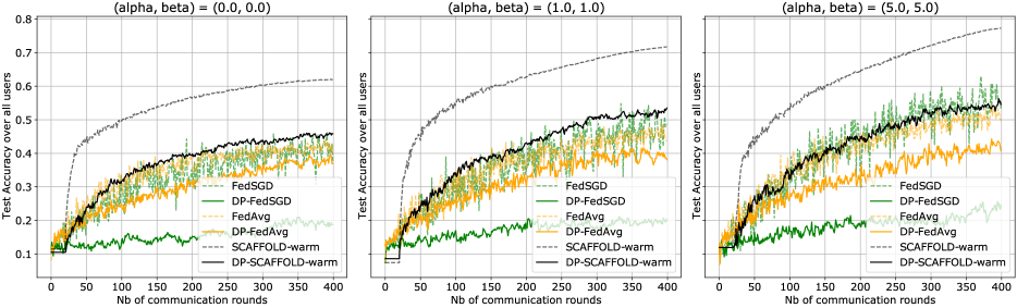
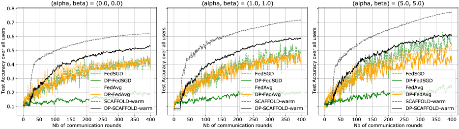
Figure 3: Test Accuracy On Synthetic Data ($\epsilon=13$). First Row: $K=50$; Second Row: $K=100$.

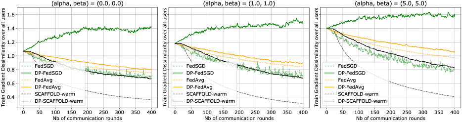
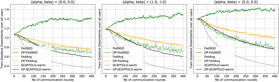
Figure 4: Train Gradient Dissimilarity On Synthetic Data ($\epsilon=13$). First Row: $K=50$; Second Row: $K=100$.

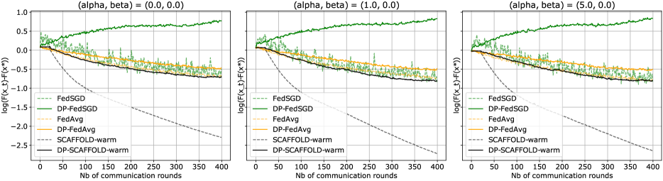
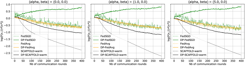
Figure 5: Model Heterogeneity (Varying $\alpha$): Train Loss On Synthetic Data ($\epsilon=13$). First Row: $K=50$; Second Row: $K=100$.

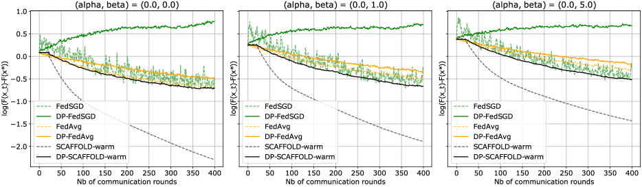
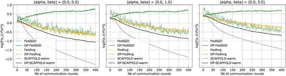
Figure 6: Data Heterogeneity Varying $\beta$): Train Loss On Synthetic Data ($\epsilon=13$). First Row: $K=50$; Second Row: $K=100$.

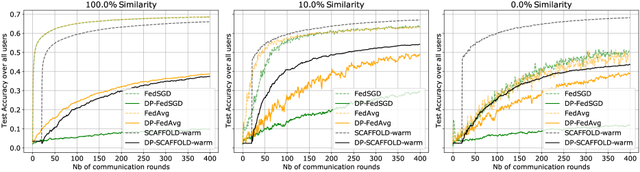
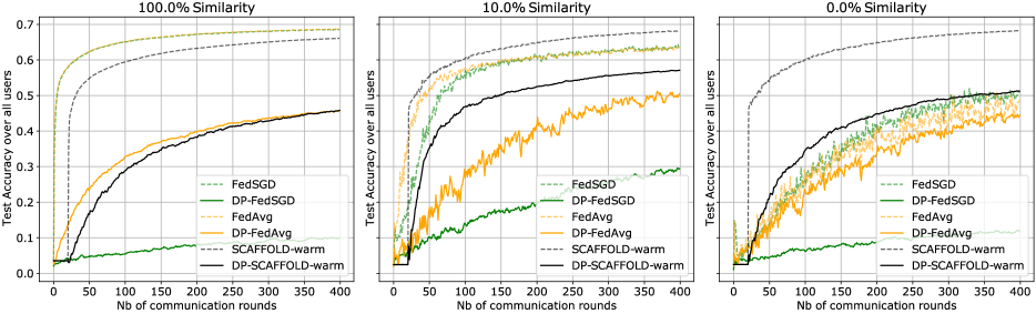
Figure 7: Test Accuracy On FEMNIST Data (LogReg) with $\epsilon=11.5$. First Row: $K=50$; Second Row: $K=100$.

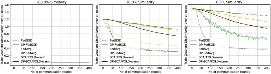
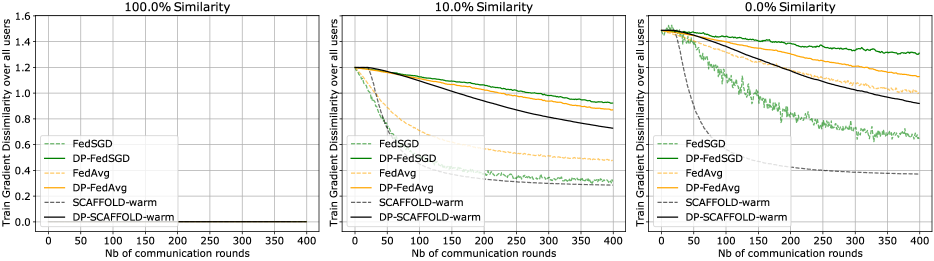
Figure 8: Train Gradient Dissimilarity On FEMNIST Data (LogReg) with $\epsilon=11.5$. First Row: $K=50$; Second Row: $K=100$.

D.3.2 Additional results on the trade-offs between $K$, $T$ and $\sigma_{g}$

In Section 5 of the main text, we presented these trade-offs for DP-SCAFFOLD under a high level of heterogeneity (see Table 1). We provide below the results of these trade-offs for DP-SCAFFOLD with a lower level of heterogeneity $(\alpha,\beta)=(0,0)$ (see Table 4). We consider again synthetic data with $\epsilon=3$ towards any third party. To report the test accuracy which is obtained at the end of the iterations, we proceed in two steps: (i) we compute the average test accuracy over the last 10% of the iterations for each random run, (ii) we calculate the mean and the standard deviation over the 3 runs and report them in the tables. We highlight in bold for each row (i.e., for each value of $\sigma_{g}$) in Tables 1,4 the best accuracy score obtained over all values of $K$.

Table 4: Test Accuracy ($\%$) For DP-SCAFFOLD On Synthetic Data $(\epsilon=3,l=0.05,s=0.2,(\alpha,\beta)=(0,0))$.

$\sigma_{g}$	$K=1$		$K=5$		$K=10$		$K=20$		$K=40$
$10$	$31.29_{\pm 0.50}$	$T=542$	$\mathbf{44.37}_{\pm 0.15}$	$T=488$	$44.17_{\pm 0.56}$	$T=428$	$41.71_{\pm 0.36}$	$T=324$	$25.92_{\pm 0.90}$	$T=72$
$20$	$28.31_{\pm 1.15}$	$T=545$	$41.97_{\pm 0.77}$	$T=502$	$\mathbf{43.27}_{\pm 0.90}$	$T=451$	$41.13_{\pm 0.55}$	$T=352$	$28.20_{\pm 2.23}$	$T=83$
$40$	$21.07_{\pm 0.41}$	$T=546$	$33.01_{\pm 1.20}$	$T=505$	$\mathbf{35.96}_{\pm 0.84}$	$T=457$	$32.82_{\pm 1.11}$	$T=360$	$23.49_{\pm 1.70}$	$T=86$
$80$	$17.09_{\pm 1.31}$	$T=546$	$21.84_{\pm 0.96}$	$T=506$	$\mathbf{25.92}_{\pm 0.59}$	$T=458$	$24.02_{\pm 1.27}$	$T=362$	$17.95_{\pm 1.14}$	$T=87$
$160$	$15.24_{\pm 1.63}$	$T=546$	$15.37_{\pm 0.28}$	$T=506$	$\mathbf{20.09}_{\pm 1.51}$	$T=458$	$18.09_{\pm 1.86}$	$T=362$	$15.38_{\pm 0.87}$	$T=87$

We observe the same trends as the ones described for Table 1 in the main text. Indeed, our results clearly show a trade-off between $T$ and $K$ for DP-SCAFFOLD under a fixed privacy budget. If $K$ is set too low or too large, the performance of the algorithm is sub-optimal either because $T$ has to be chosen too low or because control variates are inefficient under few local updates.

Moreover, we observe that setting $\sigma_{g}$ to a high value does not necessarily improve the gain in the number of communication rounds. In particular, for high values of $\sigma_{g}$, the calculation of the privacy bound does not allow to obtain a large increase in $T$ ($T$ does not change between $\sigma_{g}=40$ and $\sigma_{g}=160$ for any value of $K$), which thus leads to poor performance. This can be explained by the fact that the upper bound for the subsampled Gaussian mechanism given in Lemma B.7 does not converge to $0$ when $\sigma_{g}$ is very large. Indeed, given a subsampling ratio $q<1$, we can observe that this bound in the asymptotic regime becomes $\frac{1}{\alpha-1}\log(1+2\sum_{j=3}^{\alpha}q^{j}\binom{\alpha}{j})$, which is positive. Hence, by increasing the value of $\sigma_{g}$, we cannot hope to inconditionally increase the number of compositions of the mechanism under a fixed privacy budget, if $q$ is taken too large. This artefact thus proves how small subsampling ratios have to be chosen to compute differential privacy in practice. In our experiments, we can clearly notice that this asymptotic regime is reached as soon as $\sigma_{g}$ is greater than $80$. One would have to consider lower subsampling ratios (for instance $l=10^{-4},s=10^{-4}$), to obtain different values for $T$ when $\sigma_{g}=80$ and $\sigma_{g}=160$. We investigate such trade-offs in the next section.

D.3.3 Experiments under higher privacy regime and role of sampling parameters

In Section 5 of the main text, given private parameter $\sigma_{g}$, we conducted experiments for (i) convex objective on FEMNIST ($\sigma_{g}=30$) and synthetic data ($\sigma_{g}=60$) and (ii) non-convex objective on MNIST data ($\sigma_{g}=30$). Considering the sampling parameters we used ($l=0.2,s=0.2$), this setting allows to reach, towards any third party, $(11.4,\delta)$-DP for FEMNIST data and $(13,\delta)$-DP for synthetic data. In the case of MNIST data, we obtain $(7.2,\delta)$-DP towards any third party for $(K,T)=(50,100)$. Although these experiments only allow “low privacy”, stronger DP guarantees can be obtained by simply decreasing the subsampling ratios (thus amplifying the privacy). For instance, setting $l^{\prime}=l/4=0.05$ in case of synthetic data would provide $(4.2,\delta)$-DP for $(K,T)=(50,400)$. We present below some results on numerical trade-offs under a higher privacy regime.

As observed in the experiments of the main text and consistently with previous work (Karimireddy et al., 2020b), we observe the superiority of SCAFFOLD over FedAvg and FedSGD under heterogeneous data, but most importantly our results show that this hierarchy is preserved in our DP-FL framework with privacy constraints: this is especially clear with growing heterogeneity and with growing number $K$ of local updates. Besides this, the results provided for logistic regression in the privacy regime numerically demonstrate that DP-SCAFFOLD sometimes even outperforms (non-private) FedAvg despite the local injection of Gaussian noise, see for instance Fig. 1-10 and Fig. 2 (bottom row), and to a lesser extent Fig. 9. Therefore, our results are quite promising with respect to obtaining efficient DP-FL algorithms under heterogeneous data for higher privacy regimes.

Trade-offs between $l$ and $T$.

In this section, we compare the robustness of DP-FedAvg and DP-SCAFFOLD w.r.t. user sampling ratio $l$, under a fixed privacy bound $\epsilon$ towards a third party. We fix parameters $s=0.2,K=10$ and report in Figure 9 the evolution of the test accuracy of these algorithms for $l\in\{0.08,0.1,0.12\}$ over the communication rounds. For each value of $l$, the number of communication rounds $T_{l}$ is determined to be maximal w.r.t. to the privacy bound, so that the desired privacy level is achieved for the output after $T_{l}$ rounds. These values of $T_{l}$ are represented on Figure 9 with red vertical lines (note that the higher $l$, the lower $T_{l}$). We conduct this experiment on the following datasets: synthetic data with $\epsilon=5$ (Fig 9, first row), FEMNIST data with LogReg model, $\epsilon=5$ (Fig 9, second row) and MNIST data with DNN model, $\epsilon=3$ (Fig 9, third row).

Our results first show that DP-SCAFFOLD achieves much better performance than DP-FedAvg in these high privacy regimes. The superiority of DP-SCAFFOLD towards DP-FedAvg is especially strong under high heterogeneity: we notice a gap of 20% in the accuracy score with synthetic data for $(\alpha,\beta)=(5,5)$ and FEMNIST data for $\gamma=0\%$ with logistic regression model, a gap of 10% in the accuracy score for MNIST data with $\gamma=0\%$ and DNN. Furthermore, DP-SCAFFOLD is robust to a low value of user sampling parameter $l$. We observe that we obtain the best performance by choosing $l=0.08$ (the lowest value considered), which allows to set $T_{l}$ to a high value. Note that the evolution of the accuracy is similar for all values of $l$. Therefore, setting a low $l$ provides an effective way to achieve good accuracy with higher privacy.

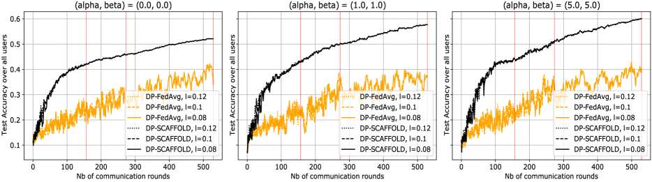
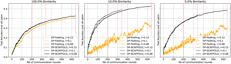
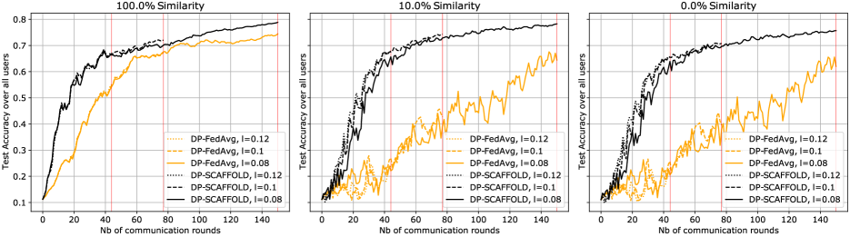
Figure 9: Test Accuracy With Various Values For $l$ Under Fixed Privacy Budget. First Row: Synthetic data ($\epsilon=5$); Second Row: FEMNIST data (LogReg, $\epsilon=5$); Third Row: MNIST (DNN, $\epsilon=3$).

Trade-offs between $s$ and $T$.

In this section, we compare the behavior of DP-FedAvg and DP-SCAFFOLD w.r.t. data sampling ratio $s$ under a fixed privacy bound $\epsilon$ towards a third party. We fix parameters $l=0.1,K=10$ and report in Figure 10 the evolution of the test accuracy of these algorithms for $s\in\{0.05,0.1,0.2\}$ over the communication rounds. For each value of $s$, the number of communication rounds $T_{s}$ is determined to be maximal w.r.t. to the privacy bound, so that the desired privacy level is achieved for the output after $T_{s}$ rounds. These values of $T_{s}$ are represented on Figure 10 with red vertical lines (note that the higher $s$, the lower $T$). We conduct this experiment for the following datasets: synthetic data with $\epsilon=5$ (Fig 10, first row), FEMNIST data with LogReg model, $\epsilon=5$ (Fig 10, second row) and MNIST data with DNN model, $\epsilon=3$ (Fig 10, third row).

Our results confirm that DP-SCAFFOLD leads to better performance than DP-FedAvg with any value of $s\in\{0.2,0.1,0.05\}$ under heterogeneity (as expected, we obtain very similar accuracy scores for these two algorithms with $\gamma=100\%$ for FEMNIST and MNIST data). However, this superiority decreases as $s$ decreases. Consider for instance FEMNIST data with 10% similarity: the gap in accuracy drops from 30% with $s=0.2$, to less than 20% with $s=0.1$. Our results seem to show that we obtain better performance with a high value of $s$, although it implies to set $T_{s}$ to a lower value. This is contrast to the effect of $l$ shown in Fig 9.

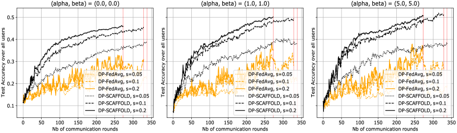
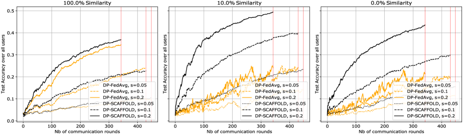
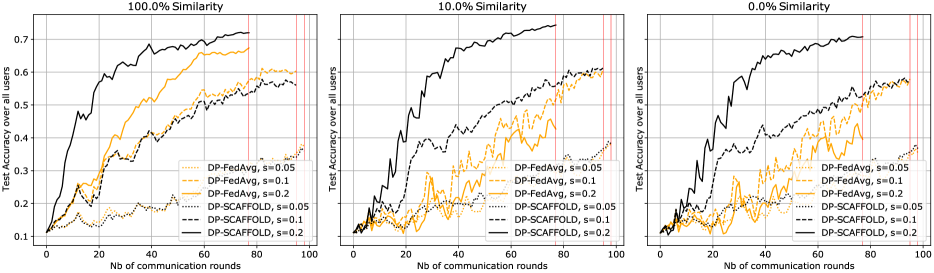
Figure 10: Test Accuracy With Various Values For $s$ Under Fixed Privacy Budget. First Row: Synthetic Data ($\epsilon=5$); Second Row: FEMNIST Data (LogReg, $\epsilon=5$); Third Row: MNIST Data (DNN, $\epsilon=3$).

References

- Abadi et al. (2016) Martin Abadi, Andy Chu, Ian Goodfellow, H Brendan McMahan, Ilya Mironov, Kunal Talwar, and Li Zhang. Deep learning with differential privacy. In Proceedings of the 2016 ACM SIGSAC conference on computer and communications security, pages 308–318, 2016.
- Acar et al. (2021) Durmus Alp Emre Acar, Yue Zhao, Ramon Matas, Matthew Mattina, Paul Whatmough, and Venkatesh Saligrama. Federated learning based on dynamic regularization. In International Conference on Learning Representations, 2021.
- Andrew et al. (2021) Galen Andrew, Om Thakkar, H. Brendan McMahan, and Swaroop Ramaswamy. Differentially private learning with adaptive clipping. Advances in Neural Information Processing Systems, 34, 2021.
- Balle et al. (2019) Borja Balle, James Bell, Adrià Gascón, and Kobbi Nissim. The privacy blanket of the shuffle model. In Annual International Cryptology Conference, pages 638–667. Springer, 2019.
- Bellet et al. (2018) Aurélien Bellet, Rachid Guerraoui, Mahsa Taziki, and Marc Tommasi. Personalized and private peer-to-peer machine learning. In International Conference on Artificial Intelligence and Statistics, pages 473–481. PMLR, 2018.
- Cheu et al. (2019) Albert Cheu, Adam Smith, Jonathan Ullman, David Zeber, and Maxim Zhilyaev. Distributed differential privacy via shuffling. In Annual International Conference on the Theory and Applications of Cryptographic Techniques, pages 375–403. Springer, 2019.
- Cohen et al. (2017) Gregory Cohen, Saeed Afshar, Jonathan Tapson, and Andre Van Schaik. Emnist: Extending mnist to handwritten letters. In 2017 international joint conference on neural networks (IJCNN), pages 2921–2926. IEEE, 2017.
- Duchi et al. (2011) John C. Duchi, Elad Hazan, and Yoram Singer. Adaptive subgradient methods for online learning and stochastic optimization. Journal of machine learning research, 12(7), 2011.
- Duchi et al. (2013) John C. Duchi, Michael I. Jordan, and Martin J. Wainwright. Local privacy and statistical minimax rates. In 2013 IEEE 54th Annual Symposium on Foundations of Computer Science, pages 429–438. IEEE, 2013.
- Duchi et al. (2018) John C. Duchi, Michael I. Jordan, and Martin J. Wainwright. Minimax optimal procedures for locally private estimation. Journal of the American Statistical Association, 113(521):182–201, 2018.
- Dwork and Roth (2014) Cynthia Dwork and Aaron Roth. The algorithmic foundations of differential privacy. Foundations and Trends® in Theoretical Computer Science, 9(3-4):211–407, 2014.
- Dwork et al. (2010) Cynthia Dwork, Guy N. Rothblum, and Salil Vadhan. Boosting and differential privacy. In 2010 IEEE 51st Annual Symposium on Foundations of Computer Science, pages 51–60. IEEE, 2010.
- Erlingsson et al. (2019) Úlfar Erlingsson, Vitaly Feldman, Ilya Mironov, Ananth Raghunathan, Kunal Talwar, and Abhradeep Thakurta. Amplification by shuffling: From local to central differential privacy via anonymity. In Proceedings of the Thirtieth Annual ACM-SIAM Symposium on Discrete Algorithms, pages 2468–2479. SIAM, 2019.
- Fallah et al. (2020) Alireza Fallah, Aryan Mokhtari, and Asuman Ozdaglar. Personalized federated learning with theoretical guarantees: A model-agnostic meta-learning approach. Advances in Neural Information Processing Systems, 33:3557–3568, 2020.
- Fredrikson et al. (2015) Matt Fredrikson, Somesh Jha, and Thomas Ristenpart. Model inversion attacks that exploit confidence information and basic countermeasures. In Proceedings of the 22nd ACM SIGSAC conference on computer and communications security, pages 1322–1333, 2015.
- Geiping et al. (2020) Jonas Geiping, Hartmut Bauermeister, Hannah Dröge, and Michael Moeller. Inverting gradients-how easy is it to break privacy in federated learning? Advances in Neural Information Processing Systems, 33:16937–16947, 2020.
- Geyer et al. (2017) Robin C. Geyer, Tassilo Klein, and Moin Nabi. Differentially private federated learning: A client level perspective. arXiv preprint arXiv:1712.07557, 2017.
- Ghazi et al. (2019) Badih Ghazi, Rasmus Pagh, and Ameya Velingker. Scalable and differentially private distributed aggregation in the shuffled model. arXiv preprint arXiv:1906.08320, 2019.
- Girgis et al. (2021a) Antonious M. Girgis, Deepesh Data, and Suhas Diggavi. Renyi differential privacy of the subsampled shuffle model in distributed learning. Advances in Neural Information Processing Systems, 34, 2021a.
- Girgis et al. (2021b) Antonious M. Girgis, Deepesh Data, Suhas Diggavi, Peter Kairouz, and Ananda Theertha Suresh. Shuffled model of federated learning: Privacy, accuracy and communication trade-offs. IEEE Journal on Selected Areas in Information Theory, 2(1):464–478, 2021b.
- Gower et al. (2019) Robert Mansel Gower, Nicolas Loizou, Xun Qian, Alibek Sailanbayev, Egor Shulgin, and Peter Richtárik. Sgd: General analysis and improved rates. In International Conference on Machine Learning, pages 5200–5209. PMLR, 2019.
- Hsu et al. (2019) Tzu-Ming Harry Hsu, Hang Qi, and Matthew Brown. Measuring the effects of non-identical data distribution for federated visual classification. arXiv preprint arXiv:1909.06335, 2019.
- Hu et al. (2020) Rui Hu, Yuanxiong Guo, Hongning Li, Qingqi Pei, and Yanmin Gong. Personalized federated learning with differential privacy. IEEE Internet of Things Journal, 7(10):9530–9539, 2020.
- Kairouz et al. (2015) Peter Kairouz, Sewoong Oh, and Pramod Viswanath. The composition theorem for differential privacy. In International conference on machine learning, pages 1376–1385. PMLR, 2015.
- Kairouz et al. (2021) Peter Kairouz, H. Brendan McMahan, Brendan Avent, Aurélien Bellet, Mehdi Bennis, Arjun Nitin Bhagoji, Kallista Bonawitz, Zachary Charles, Graham Cormode, Rachel Cummings, Rafael G. L. D’Oliveira, Hubert Eichner, Salim El Rouayheb, David Evans, Josh Gardner, Zachary Garrett, Adrià Gascón, Badih Ghazi, Phillip B. Gibbons, Marco Gruteser, Zaid Harchaoui, Chaoyang He, Lie He, Zhouyuan Huo, Ben Hutchinson, Justin Hsu, Martin Jaggi, Tara Javidi, Gauri Joshi, Mikhail Khodak, Jakub Konečný, Aleksandra Korolova, Farinaz Koushanfar, Sanmi Koyejo, Tancrède Lepoint, Yang Liu, Prateek Mittal, Mehryar Mohri, Richard Nock, Ayfer Özgür, Rasmus Pagh, Mariana Raykova, Hang Qi, Daniel Ramage, Ramesh Raskar, Dawn Song, Weikang Song, Sebastian U. Stich, Ziteng Sun, Ananda Theertha Suresh, Florian Tramèr, Praneeth Vepakomma, Jianyu Wang, Li Xiong, Zheng Xu, Qiang Yang, Felix X. Yu, Han Yu, and Sen Zhao. Advances and open problems in federated learning. Foundations and Trends® in Machine Learning, 14(1–2):1–210, 2021.
- Karimireddy et al. (2020a) Sai Praneeth Karimireddy, Martin Jaggi, Satyen Kale, Mehryar Mohri, Sashank J. Reddi, Sebastian U. Stich, and Ananda Theertha Suresh. Mime: Mimicking centralized stochastic algorithms in federated learning. arXiv preprint arXiv:2008.03606, 2020a.
- Karimireddy et al. (2020b) Sai Praneeth Karimireddy, Satyen Kale, Mehryar Mohri, Sashank Reddi, Sebastian Stich, and Ananda Theertha Suresh. Scaffold: Stochastic controlled averaging for federated learning. In International Conference on Machine Learning, pages 5132–5143. PMLR, 2020b.
- Kasiviswanathan et al. (2011) Shiva Prasad Kasiviswanathan, Homin K Lee, Kobbi Nissim, Sofya Raskhodnikova, and Adam Smith. What can we learn privately? SIAM Journal on Computing, 40(3):793–826, 2011.
- Khaled et al. (2020) Ahmed Khaled, Konstantin Mishchenko, and Peter Richtárik. Tighter theory for local sgd on identical and heterogeneous data. In International Conference on Artificial Intelligence and Statistics, pages 4519–4529. PMLR, 2020.
- Kingma and Ba (2014) Diederik P. Kingma and Jimmy Ba. Adam: A method for stochastic optimization. arXiv preprint arXiv:1412.6980, 2014.
- LeCun et al. (1998) Yann LeCun, Léon Bottou, Yoshua Bengio, and Patrick Haffner. Gradient-based learning applied to document recognition. Proceedings of the IEEE, 86(11):2278–2324, 1998.
- Li et al. (2020a) Tian Li, Anit Kumar Sahu, Manzil Zaheer, Maziar Sanjabi, Ameet Talwalkar, and Virginia Smith. Federated optimization in heterogeneous networks. Proceedings of Machine Learning and Systems, 2:429–450, 2020a.
- Li et al. (2020b) Yiwei Li, Tsung-Hui Chang, and Chong-Yung Chi. Secure federated averaging algorithm with differential privacy. In 2020 IEEE 30th International Workshop on Machine Learning for Signal Processing (MLSP), pages 1–6. IEEE, 2020b.
- Marfoq et al. (2021) Othmane Marfoq, Giovanni Neglia, Aurélien Bellet, Laetitia Kameni, and Richard Vidal. Federated multi-task learning under a mixture of distributions. Advances in Neural Information Processing Systems, 34, 2021.
- McMahan et al. (2017) H. Brendan McMahan, Eider Moore, Daniel Ramage, Seth Hampson, and Blaise Aguera y Arcas. Communication-efficient learning of deep networks from decentralized data. In Artificial intelligence and statistics, pages 1273–1282. PMLR, 2017.
- McMahan et al. (2018) H. Brendan McMahan, Daniel Ramage, Kunal Talwar, and Li Zhang. Learning differentially private recurrent language models. In International Conference on Learning Representations, 2018.
- Mironov (2017) Ilya Mironov. Rényi differential privacy. In 2017 IEEE 30th computer security foundations symposium (CSF), pages 263–275. IEEE, 2017.
- Nesterov et al. (2004) Yurii Nesterov et al. Lectures on convex optimization, volume 137. Springer, 2004.
- Reddi et al. (2020) Sashank J. Reddi, Zachary Charles, Manzil Zaheer, Zachary Garrett, Keith Rush, Jakub Konečnỳ, Sanjiv Kumar, and H. Brendan McMahan. Adaptive federated optimization. In International Conference on Learning Representations, 2020.
- Sattler et al. (2020) Felix Sattler, Klaus-Robert Müller, and Wojciech Samek. Clustered federated learning: Model-agnostic distributed multitask optimization under privacy constraints. IEEE Transactions on Neural Networks and Learning Systems, 2020.
- Shokri et al. (2017) Reza Shokri, Marco Stronati, Congzheng Song, and Vitaly Shmatikov. Membership inference attacks against machine learning models. In 2017 IEEE Symposium on Security and Privacy (SP), pages 3–18. IEEE, 2017.
- Triastcyn and Faltings (2019) Aleksei Triastcyn and Boi Faltings. Federated learning with bayesian differential privacy. In 2019 IEEE International Conference on Big Data (Big Data), pages 2587–2596. IEEE, 2019.
- Van Erven and Harremos (2014) Tim Van Erven and Peter Harremos. Rényi divergence and kullback-leibler divergence. IEEE Transactions on Information Theory, 60(7):3797–3820, 2014.
- Wang et al. (2021) Jianyu Wang, Zachary Charles, Zheng Xu, Gauri Joshi, H. Brendan McMahan, Maruan Al-Shedivat, Galen Andrew, Salman Avestimehr, Katharine Daly, Deepesh Data, et al. A field guide to federated optimization. arXiv preprint arXiv:2107.06917, 2021.
- Wang et al. (2020) Yu-Xiang Wang, Borja Balle, and Shiva Kasiviswanathan. Subsampled Rényi Differential Privacy and Analytical Moments Accountant. Journal of Privacy and Confidentiality, 10(2), 2020.
- Wei et al. (2020) Kang Wei, Jun Li, Ming Ding, Chuan Ma, Howard H. Yang, Farhad Farokhi, Shi Jin, Tony Q. S. Quek, and H. Vincent Poor. Federated learning with differential privacy: Algorithms and performance analysis. IEEE Transactions on Information Forensics and Security, 15:3454–3469, 2020.
- Zhao et al. (2021) Yang Zhao, Jun Zhao, Mengmeng Yang, Teng Wang, Ning Wang, Lingjuan Lyu, Dusit Niyato, and Kwok-Yan Lam. Local Differential Privacy based Federated Learning for Internet of Things. IEEE Internet of Things Journal, 8(11):8836–8853, 2021.
Supplementary Material:
Differentially Private Federated Learning on Heterogeneous Data