SmoothMix: Training Confidence-calibrated Smoothed Classifiers for Certified Robustness

Abstract

Randomized smoothing is currently a state-of-the-art method to construct a certifiably robust classifier from neural networks against $\ell_{2}$-adversarial perturbations. Under the paradigm, the robustness of a classifier is aligned with the prediction confidence, i.e., the higher confidence from a smoothed classifier implies the better robustness. This motivates us to rethink the fundamental trade-off between accuracy and robustness in terms of calibrating confidences of a smoothed classifier. In this paper, we propose a simple training scheme, coined SmoothMix, to control the robustness of smoothed classifiers via self-mixup: it trains on convex combinations of samples along the direction of adversarial perturbation for each input. The proposed procedure effectively identifies over-confident, near off-class samples as a cause of limited robustness in case of smoothed classifiers, and offers an intuitive way to adaptively set a new decision boundary between these samples for better robustness. Our experimental results demonstrate that the proposed method can significantly improve the certified $\ell_{2}$-robustness of smoothed classifiers compared to existing state-of-the-art robust training methods.

1 Introduction

Adversarial examples [53, 17] in deep neural networks clearly highlight that neural networks often generalize differently from humans, at least without an additional prior of local smoothness of predictions with respect to the input space: an adversarially-crafted, yet imperceptible input perturbation can drastically change the prediction of a neural network based classifier. Due to the intrinsic complexity of neural networks, however, the community has noticed that it is extremely hard to directly encode this smoothness prior into neural networks [6, 3, 55], especially without relying on adversarial training [40, 66], i.e., augmenting training data with its adversarial examples. Even with adversarial training, (a) the non-convex, minimax nature of the training introduces many optimization difficulties, often resulting in a harsh over-fitting [51, 47], and (b) it is generally hard to provably guarantee that the learned classifier is indeed smooth.

Randomized smoothing [33, 11] is relatively a recent idea that aims to indirectly encode the smoothness prior: Cohen et al. [11] have shown that any classifier, regardless of whether it is smooth or not, can be transformed into a certifiably robust classifier via averaging its predictions over Gaussian noise, where the (certified) robustness of the classifier depends on how well the base classifier performs with the noise. Compared to adversarial training, this notion of “indirect” smoothness can be favorable in a sense that (a) it is easier to optimize, and (b) offers a provable guarantee on the robustness. Currently, randomized smoothing is considered as the state-of-the-art approach in the context of building a neural network based classifier that is certifiably robust on $\ell_{2}$-perturbations [39].

In this respect, a growing body of research has focused on improving the robustness guarantee that randomized smoothing can give, e.g., via different smoothing measures [34, 62] or improved certification procedures [14, 43]. One of important directions on this line of research is to investigate which training of the base classifier could maximize the certified robustness of smoothed classifiers [49, 65, 23]. In particular, Salman et al. [49] have proposed SmoothAdv, showing that employing adversarial training [40] for smoothed classifiers could further improve the robustness, akin to the standard neural networks. This motivates us to develop a new form of adversarial training, more specialized for smoothed classifiers.

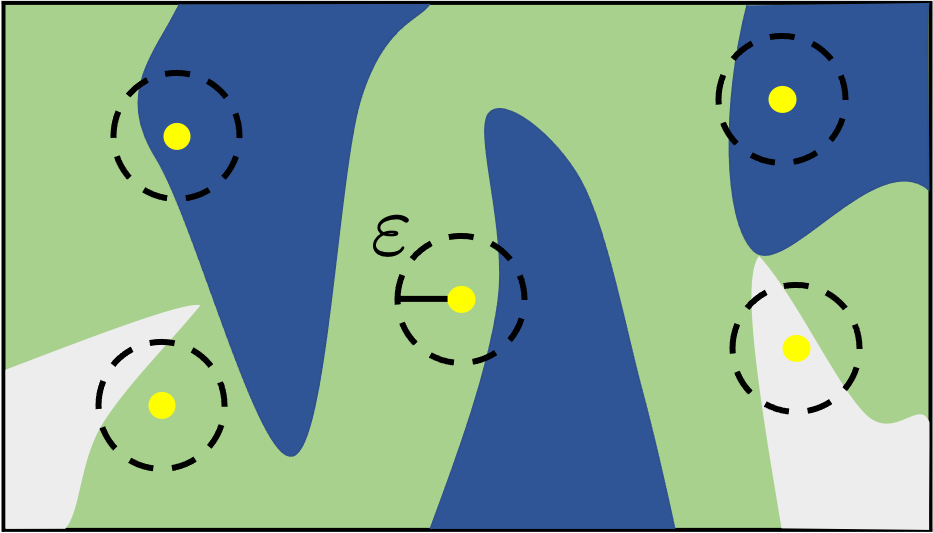
(a) Adversarial training [40]

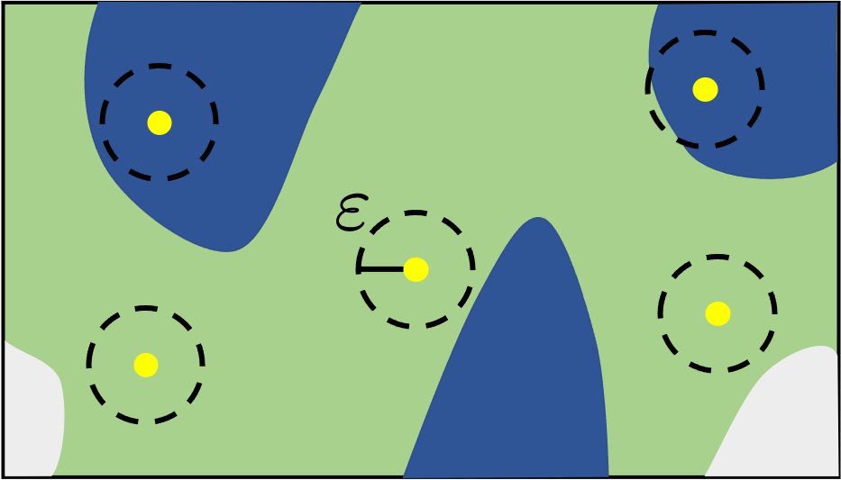
(b) SmoothAdv [49]

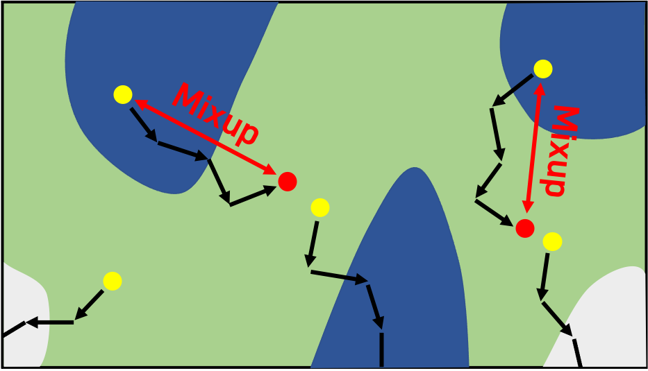
(c) SmoothMix (Ours)

Figure 1: Illustrations of how each training method obtains adversarial robustness: adversarial training [40] considers an $\varepsilon$-ball around each sample and corrects adversarial examples found in these balls; SmoothAdv [49] directly employs adversarial training on smoothed classifiers; SmoothMix (ours) can be differentiated from SmoothAdv as it (i) does not assume an explicit norm restriction on adversarial examples, and (ii) applies mixup [67] instead of correcting the adversarial examples.

Contribution. In this paper, we propose SmoothMix, a novel adversarial training method designed for improving the certified robustness of smoothed classifiers. One of the key features that smoothed classifiers offer is a direct correspondence from prediction confidence to adversarial robustness: achieving a higher confidence in a smoothed classifier implies that the classifier can give a better certified robustness. Inspired by this, we found that the certified robustness of a given data sample can be significantly decreased by nearby off-class but over-confident [45] inputs: such “harmful” inputs would occupy an unnecessarily large robust radius near the sample of our interest, especially when they do not contain much information to be discriminated by the classifier.

Under the finding, we aim to calibrate the confidence of these off-class inputs to improve the certified robustness at the original input. More specifically, we first observe that such over-confident examples can be efficiently found along the direction of adversarial perturbations for a given input. Then, we suggest to regularize the over-confident predictions along the adversarial direction toward the uniform prediction through a mixup loss [67] (see Figure 1 for an overview). This new approach of incorporating adversarial examples effectively permits more distant examples in training, even when they go off-class, based on the local-smoothness of smoothed classifiers. It also suggests an intuitive way of defining confidence beyond the given data samples to smoothed classifiers.

We evaluate our proposed SmoothMix against with various state-of-the-art robust training methods for smoothed classifiers on a wide range of image classification benchmarks, including MNIST [32], CIFAR-10 [29], and ImageNet [48] datasets. Overall, the results consistently show that our new adversarial training scheme for smoothed classifiers significantly improves the certified robustness compared to existing methods, e.g., one of our CIFAR-10 model could largely outperform an existing state-of-the-art result on the average certified robustness in $\ell_{2}$-radius $0.720\rightarrow 0.737$. Through an extensive ablation study, we also verify that our method is (a) robust to the choice of hyperparameters, and (b) can effectively trade-off between the accuracy and robustness [66] of smoothed classifiers.

Overall, our work suggests that the robustness of a classifier should be set individually per sample considering its nearby inputs: we approach this problem by leveraging the relationship between the prediction confidence and robustness of smoothed classifiers. Recently, there have been also some initial attempts to incorporate a sample-wise treatment for robustness by allowing input-dependent noise scales in randomized smoothing [1, 58, 10]. However, our theoretical analysis shows that such an approach would eventually suffer from the curse of dimensionality (Theorem 1 in Appendix B), highlighting our approach of focusing on a “better calibration” as a promising alternative.

2 Preliminaries

We assume an i.i.d. dataset $\mathcal{D}=\{(x_{i},y_{i})\}^{n}_{i=1}\sim P$, where $x_{i}\in\mathbb{R}^{d}$ and $y_{i}\in\mathcal{Y}:=\{1,\cdots,C\}$, and focus on the problem of correctly classifying a given input $x$ into one of $C$ classes. Let $f:\mathbb{R}^{d}\rightarrow\mathcal{Y}$ be a classifier modeled by $f(x):=\operatorname*{arg\,max}_{c\in\mathcal{Y}}F_{c}(x)$ with $F:\mathbb{R}^{d}\rightarrow\Delta^{C-1}$, where $\Delta^{C-1}$ denotes the probability simplex in $\mathbb{R}^{C}$. For example, $F$ can be a neural network followed by a softmax layer.

In the context of adversarial robustness, we require $f$ not only to correctly classify $(x,y)\sim P$, but also to be locally-constant around $x$, i.e., $f$ should not contain any adversarial examples around $x$. In this respect, one can measure and attempt to maximize the adversarial robustness of a classifier $f$ by considering the minimum-distance of adversarial perturbation [44, 7, 8], namely:

$$R(f;x,y):=\min_{f(x^{\prime})\neq y}\|x^{\prime}-x\|_{2}.$$ (1)

Randomized smoothing. In cases when $f$ is too complex to control its predictions in practice, e.g., if $f$ is a neural network on high-dimensional data, directly solving and maximizing (1) can be hard. Randomized smoothing [11] instead constructs a new classifier $\hat{f}$ from $f$ that is easier to obtain robustness by transforming the base classifier $f$ with a certain smoothing measure, where in this paper we focus on the case of Gaussian distributions $\mathcal{N}(0,\sigma^{2}I)$:

$$\hat{f}(x):=\operatorname*{arg\,max}_{c\in\mathcal{Y}}\mathbb{P}_{\delta\sim\mathcal{N}(0,\sigma^{2}I)}\left(f(x+\delta)=c\right).$$ (2)

For a given $(x,y)$, Cohen et al. [11] have shown that $R(\hat{f};x,y)$ can be lower-bounded by the certified radius $\underline{R}(\hat{f},x,y)$, which can be derived from the confidence of $\hat{f}$ at $x$, namely we denote it by $p_{f}(x)$:

$$R(\hat{f};x,y)\geq\sigma\cdot\Phi^{-1}(p_{f}(x))=:\underline{R}(\hat{f},x,y)~{}\text{where}~{}p_{f}(x):=\mathbb{P}_{\delta\sim\mathcal{N}(0,\sigma^{2}I)}(f(x+\delta)=\hat{f}(x)),$$ (3)

provided that $\hat{f}(x)=y$, and otherwise $R(\hat{f};x,y):=0$. This lower bound is known as tight for the $\ell_{2}$-minimum distance, e.g., the bound is optimal for linear classifiers [11].

Although randomized smoothing can be applied for any classifier $f:\mathbb{R}^{d}\rightarrow\mathcal{Y}$, the robustness of smoothed classifiers can vary depending on $p_{f}$ as in (3), i.e., how $f$ performs on a given input under the presence of Gaussian noise. In this sense, to obtain a robust $\hat{f}$, Cohen et al. [11] simply propose to train $f$ using Gaussian augmentation by default:

$$\min_{F}\ \mathbb{E}_{\begin{subarray}{c}(x,y)\sim P\\ \delta\sim\mathcal{N}(0,\sigma^{2}I)\end{subarray}}\left[\mathcal{L}(F(x+\delta),y)\right],$$ (4)

where $\mathcal{L}$ denotes the standard cross-entropy loss.

Adversarial training for smoothed classifiers. To obtain $f$ that gives a more robust classifier when smoothed into $\hat{f}$, Salman et al. [49] propose SmoothAdv that employs adversarial training [40] on $\hat{f}$:

$$\min_{\hat{f}}\max_{\|x^{\prime}-x\|_{2}\leq\epsilon}\mathcal{L}(\hat{f};x^{\prime},y).$$ (5)

Due to the intractability of $\hat{f}$, however, it is hard to directly optimize the inner maximization of (5) via gradient methods. To bypass this, SmoothAdv attacks the soft-smoothed classifier $\hat{F}:=\mathbb{E}_{\delta}[F_{y}(x+\delta)]$ instead. Specifically, SmoothAdv finds an adversarial example via solving the following:

$$\hat{x}=\operatorname*{arg\,max}_{\|x^{\prime}-x\|_{2}\leq\epsilon}\mathcal{L}(\hat{F};x^{\prime},y)\approx\operatorname*{arg\,max}_{\|x^{\prime}-x\|_{2}\leq\epsilon}\left(-\log\left(\frac{1}{m}\sum_{i}F_{y}(x^{\prime}+\delta_{i})\right)\right),$$ (6)

using Monte Carlo integration with $m$ samples of $\delta$, namely $\delta_{1},\cdots,\delta_{m}\sim\mathcal{N}(0,\sigma^{2}I)$.

3 Method

Our goal in this paper is to develop a more suitable form of adversarial training (AT) for smoothed classifiers, taking into account their unique characteristics on adversarial robustness over standard neural networks. Figure 1 illustrates a motivating example: as shown in Figure 1(a), AT typically assumes a fixed-sized ball of radius $\varepsilon$ that each adversarial perturbation must be in, as the goal of the training is to defend the classifier against adversaries under a specific threat model. However, in a case when AT is applied to a smoothed classifier, e.g., as done by SmoothAdv, this assumption may be too restrictive, particularly for inputs where the classifier already certifies robustness of radii larger than $\varepsilon$ (e.g., Figure 1(b)). This demands for a new form of AT specially for smoothed classifiers, e.g., that allows more distant adversarial examples, despite its fundamental difficulty in the context of standard neural networks [25, 69].

In this regard, our proposed training method of SmoothMix takes a completely different approach to incorporate adversarial examples during training. More specifically, for a given sample $(x,y)\sim P$, our method finds an adversarial example of $x$ without an explicit norm constraint, i.e., “unrestrictively.” This is because our focus is not to find an input for correcting its label to $y$ (as in the standard AT), but to find an input that is over-confident and semantically off-class, i.e., it is not beneficial to the classifier to label this input to $y$. Once we have such an example, SmoothMix then labels it as the uniform confidence, and considers a mixup training [67] with the original $x$: by linearly interpolating with the uniform confidence, SmoothMix effectively calibrates the over-confident inputs in between, re-balancing the certified radius at the original sample of $x$ at the end.

3.1 Exploring over-confident adversarial examples in smoothed classifiers

Recall that we have a (base) classifier $f$ of the form $f(x)=\operatorname*{arg\,max}_{c\in\mathcal{Y}}F_{c}(x)$, $\hat{f}$ is its smoothed counterpart, and we aim to improve the robustness of $\hat{f}$ by incorporating adversarial examples in training. In this paper, we are particularly interested in adversarial examples of $\hat{f}$ that is found without a hard restriction in its perturbation size. More concretely, for a given training sample $(x,y)\sim P$, we find adversarial examples by solving the following optimization:

$$\tilde{x}:=\operatorname*{arg\,max}_{x^{\prime}}\left({\mathcal{L}(\hat{f};x^{\prime},y)-\beta\cdot\|x^{\prime}-x\|_{2}^{2}}\right),$$ (7)

where $\mathcal{L}$ is the cross-entropy loss, and $\beta>0$ is to ensure that (7) cannot be arbitrarily far from $x$.

As proposed by Salman et al. [49] (see Section 2), one can optimize (7) by approximating the intractable $\hat{f}$ with the soft-smoothed classifier $\hat{F}:=\mathbb{E}_{\delta}[F(x+\delta)]$, in a similar manner to (6). Based on this approximation, we simply perform a $T$-step gradient ascent from $\tilde{x}^{(0)}:=x$ with step size $\alpha>0$ to solve (7) using $m$ samples of $\delta$, namely $\delta_{1},\cdots,\delta_{m}\sim\mathcal{N}(0,\sigma^{2}I)$:

$$\tilde{x}^{(t+1)}:=\tilde{x}^{(t)}+\alpha\cdot\frac{\nabla_{x}J(\tilde{x}^{(t)})}{\|\nabla_{x}J(\tilde{x}^{(t)})\|_{2}},\text{ where \ }J(x):=-\log\left(\frac{1}{m}\sum_{i}F_{y}(x+\delta_{i})\right).$$ (8)

Figure 3 demonstrates two particular instances of these “unrestricted” adversarial examples found from (8) on $x$, and plots how the confidence of inputs changes as they are linearly interpolated from the clean input to its adversarial counterpart. From this illustration, we make several remarks those would lead to a more direct motivation to our method:

• We observe that adversarial perturbations found via (8), i.e., from a smoothed classifier, could contain enough amount of semantic changes even in a perceptual sense, in either ways of translating the input to another class (Figure 2(a)), or simply removing some relevant information for the current class (Figure 2(b)). At least for these cases, therefore, it is reasonable for the classifier to keep its low confidence to the original class. Such a “perceptually-aligned” representation is not a unique property of smoothed classifiers, but has been generally observed on adversarially-robust classifiers [50, 15, 26]: in other words, we leverage the provable robustness of smoothed classifiers during training to reasonably obtain a semantically off-class samples, those will be labeled as the uniform confidence.

• A major problem we rather highlight here is the tendency of over-confidence [45] toward the direction of adversarial perturbation: Figure 3 also presents how the confidence of the given smoothed classifier changes as we linearly interpolate the input from $x$ to $\tilde{x}$. Overall, the adversarially-crafted samples $\tilde{x}$ usually attain significantly higher confidence compared to that of $x$, consequently their certified radius (3) would be much larger as well. Therefore, considering that $\tilde{x}$ are still nearby $x$, such the over-confidence at $\tilde{x}$ would negatively affect the certified radius of $x$, especially when $\tilde{x}$ does not contain much semantically meaningful information as observed in Figure 2(b). This observation is further supported qualitatively in Table 1: by comparing the average (a) true-class confidence and their (b) off-class confidences of a smoothed classifier, those are defined by (a) $\mathbb{E}[\mathbb{P}(f(x+\delta)=y)]$ and (b) $\mathbb{E}[\max_{c\neq y}\mathbb{P}(f(x+\delta)=c)]$, respectively, we confirm that the off-class confidence of $\tilde{x}$ can be abnormally higher than those of clean samples $x$ as we allow more budget on $\varepsilon$.

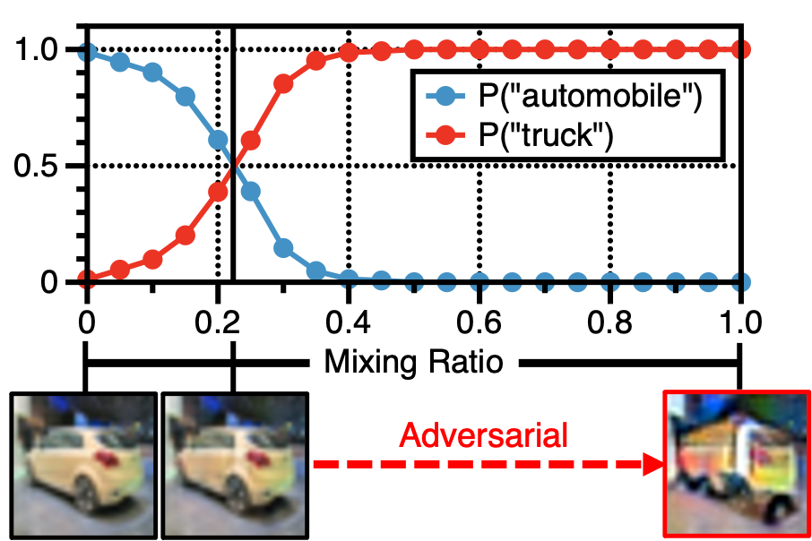
(a) In-class translation

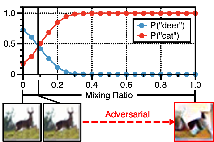
(b) Out-of-class translation

Figure 2: Illustration of adversarial examples unrestrictively found in CIFAR-10 with a smoothed ResNet-110 ($\sigma=0.25$). The plot demonstrates the change of confidence between two classes as the input is linearly interpolated.

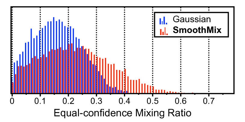
Figure 3: Equal-confidence mixing ratios on CIFAR-10, i.e., the minimal mixing ratios for changing the correct prediction when each input is linearly interpolated to its adversarial example.

Table 1: Comparison of the average (a) true-class confidence, and (b) maximum off-class confidence of smoothed classifiers, for adversarial inputs searched via PGD from CIFAR-10 test samples around $\ell_{2}$-ball of radius $\varepsilon$. We use ResNet-110 trained on CIFAR-10 with $\sigma=0.5$ for this comparison.

CIFAR-10 (Test set; %)	Clean	$\varepsilon=1.0$	$\varepsilon=2.0$	$\varepsilon=3.0$	$\varepsilon=4.0$	$\varepsilon=5.0$
(a) $\mathbb{E}[\mathbb{P}(f(x+\delta)=y)]$	66.4	47.1	24.3	14.2	11.3	10.7
(b) $\mathbb{E}[\max_{c\neq y}\mathbb{P}(f(x+\delta)=c)]$	24.2	37.8	59.5	71.8	78.5	82.0

3.2 SmoothMix for confidence-calibrated training of smoothed classifiers

Based on the observations from Section 3.1, we hypothesize that the miscalibration of confidences between $x$ and its unrestricted adversarial example $\tilde{x}$ is an important factor that degrades the certified robustness of smoothed classifiers, and propose to penalize the over-confidence by mixing the uniform confidence to them. More concretely, we consider the mixup [67] training between $x$ and $\tilde{x}$, i.e., by augmenting the given training data with the following pairs:

$$x^{\tt mix}:=(1-\lambda)\cdot x+\lambda\cdot\tilde{x}^{(T)},y^{\tt mix}:=(1-\lambda)\cdot\hat{F}(x)+\lambda\cdot\tfrac{\mathbbm{1}}{C},\text{ where \ }\lambda\sim\mathcal{U}\left(\left[0,\tfrac{1}{2}\right]\right)$$ (9)

where $\hat{F}(x)\in\Delta^{C-1}$ is the soft-smoothed prediction of $x$, $\mathcal{U}$ denotes the uniform distribution, $\lambda$ is a random variable that represents the mixing ratio between $(x,\hat{F}(x))$ and $(\tilde{x}^{(T)},\mathcal{U}(\mathcal{Y}))$, and $\mathbbm{1}$ denotes the $C$-dimensional vector of ones. Here, we notice that $\lambda$ is sampled only from $[0,\tfrac{1}{2}]$, unlike the standard choice [67] of $\mathcal{U}([0,1])$: recall from Figure 2(a) that $\tilde{x}$ can be often semantically in-class, so that a direct supervision of the uniform confidence on it could harm the classifier. By simply taking only the half part of the mixed samples closer to $x$, we could reasonably avoid these cases while maintaining its effect to prevent the over-confidence issue. The actual loss to minimize for these new data simply follows the cross-entropy loss with Gaussian augmentation, similarly to (4):

$$L^{\tt mix}:=\mathbb{E}_{\delta\sim\mathcal{N}(0,\sigma^{2}I)}\left[\mathcal{L}(F(x^{\tt mix}+\delta),y^{\tt mix})\right].$$ (10)

Recall the over-confidence issue observed in Figure 3 as we follow from $x$ to $\tilde{x}^{(T)}$. Minimizing $L^{\tt mix}$ (10) directly corresponds to calibrating the high confidence at $\tilde{x}^{(T)}$ and the samples in-between, while keeping the original prediction of $\hat{F}(x)$ at $x$. Even in cases that $\tilde{x}^{(T)}$ does not have an over-confidence issue, i.e., when its prediction is already close to the uniform confidence, the loss (10) would assign a relatively low value for $\tilde{x}^{(T)}$ so that it can act only if there exists an overconfident $\tilde{x}^{(T)}$ nearby $x$.

Incorporating SmoothAdv for free. As our method focuses on adversarial examples that are moderately far from the original inputs assuming that the classifier is already locally-smooth, one may still enjoy the effectiveness of SmoothAdv if it could further enforce the local smoothness. We indeed observe that the joint training can be helpful for the robustness of smoothed classifiers, but a naïve combination of them could incur too much costs for finding separate adversarial examples for each method. Instead, we found that simply taking $x\leftarrow\tilde{x}^{(1)}$ without modifying our current training, i.e., using the single-step adversarial example found during (8) instead of the clean sample, can reasonably bring a similar effect. In this respect, we allow SmoothMix to use $(\tilde{x}^{(1)},y)$ instead of $(x,y)$ depending on demand of more robustness at expense of decreased clean accuracy.

Overall training. Combining the proposed loss with the standard Gaussian training (4) gives the full objective to minimize for our training method. For a given sample $(x,y)\sim P$, and by letting $L^{\tt nat}:=\mathbb{E}_{\delta}\left[\mathcal{L}(F(x+\delta),y)\right]$, the final loss of SmoothMix is given by:

$$L:=L^{\tt nat}+\eta\cdot L^{\tt mix},$$ (11)

where $\eta>0$ is a hyperparameter to control the trade-off between accuracy and robustness. Algorithm 1 in Appendix A demonstrates a concrete training procedure of SmoothMix using $m$ samples of $\delta$ for the Monte Carlo approximation.

4 Experiments

We evaluate the effectiveness of our method extensively on MNIST [32], CIFAR-10 [29], and ImageNet [48] classification datasets. Overall, the results consistently highlight that our newly proposed training can significantly improve the certified robustness of smoothed classifiers compared to existing robust training methods. We point out the improvements are especially remarkable on the certified accuracy at larger perturbations, at which SmoothMix mainly focus compared to prior arts. We also conduct an ablation study on the proposed method to convey a detailed analysis on the individual components. The detailed experimental setups, e.g., training details, datasets, and hyperparameters for the baseline methods, are specified in Appendix C.

Baseline methods. We compare our method with a variety of existing techniques proposed for a robust training of smoothed classifiers, as listed in what follows: (a) Gaussian [11]: standard training with Gaussian augmentation; (b) Stability training [38]: a cross-entropy regularization between $F(x)$ and $F(x+\delta)$; (c) SmoothAdv [49]: adversarial training on smoothed classifier; (d) MACER [65]: a regularization that maximizes an approximative form of the certified radius (3); and (e) Consistency [23]: a KL-divergence based regularization that minimizes the variance of $F(x+\delta)$ across $\delta$. Whenever possible, we use the pre-trained models released by authors for our evaluation to reproduce the baselines. The more detailed training configurations are specified in Appendix C.2.

Evaluation metrics. Our evaluation of the robustness for a given smoothed classifier $\hat{f}$ is largely based on the protocol proposed by Cohen et al. [11], similarly to prior works [49, 65, 23]: more concretely, Cohen et al. [11] proposed a practical Monte Carlo based certification procedure, namely Certify, that returns the prediction of $\hat{f}$ and a “safe” lower bound of certified radius over the randomness of $n$ samples with probability at least $1-\alpha$, or abstains the certification.

From Certify, we consider two evaluation metrics: (a) the approximate certified test accuracy at various radii: the fraction of the test dataset which Certify classifies correctly with radius larger than $r$ without abstaining, and (b) the average certified radius (ACR) [65]: the average of certified radii returned by Certify on the test dataset counting only the correctly classified samples, namely $\mathrm{ACR}:=\frac{1}{|\mathcal{D}_{\tt test}|}\sum_{(x,y)\in\mathcal{D}_{\tt test}}\mathrm{CR}(f,\sigma,x)\cdot\mathbf{1}_{\hat{f}(x)=y}$, where $\mathcal{D}_{\tt test}$ is the test dataset, and $\mathrm{CR}$ denotes the certified radius from $\textsc{Certify}(f,\sigma,x)$. Here, the latter metric, ACR, is for a better comparison of robustness under trade-off between accuracy and robustness [56, 66]: by its definition, ACR naturally assigns 0 for the incorrectly classified test samples, i.e., when $\hat{f}(x)\neq y$, so that a decreased clean accuracy of $\hat{f}$ would negatively affect the value of ACR. We use the official PyTorch implementation of Certify, with $n=100,000$, $n_{0}=100$ and $\alpha=0.001$, following [11, 49, 23].

Table 2: Comparison of approximate certified test accuracy (%) and ACR on MNIST. All the models are trained and evaluated with the same smoothing factor specified by $\sigma$. Each value except ACR indicates the fraction of test samples which have $\ell_{2}$ certified radius larger than the threshold specified at the top row. We set our results bold-faced whenever the value improves the Gaussian baseline, and underlined whenever the value improves the best among the considered baselines.

$\sigma$ Models (MNIST) ACR 0.00 0.25 0.50 0.75 1.00 1.25 1.50 1.75 2.00 2.25 2.50 2.75 0.25 Gaussian [11] 0.911 99.2 98.5 96.7 93.3 0.0 0.0 0.0 0.0 0.0 0.0 0.0 0.0 Stability training [38] 0.915 99.3 98.6 97.1 93.8 0.0 0.0 0.0 0.0 0.0 0.0 0.0 0.0 SmoothAdv [49] 0.932 99.4 99.0 98.2 96.8 0.0 0.0 0.0 0.0 0.0 0.0 0.0 0.0 MACER [65] 0.920 99.3 98.7 97.5 94.8 0.0 0.0 0.0 0.0 0.0 0.0 0.0 0.0 Consistency [23] 0.928 99.5 98.9 98.0 96.0 0.0 0.0 0.0 0.0 0.0 0.0 0.0 0.0 SmoothMix ($\eta=1.0$) 0.931 99.5 98.9 98.2 96.4 0.0 0.0 0.0 0.0 0.0 0.0 0.0 0.0 + One-step adversary 0.933 99.4 99.0 98.2 96.9 0.0 0.0 0.0 0.0 0.0 0.0 0.0 0.0 SmoothMix ($\eta=5.0$) 0.932 99.4 99.0 98.2 96.7 0.0 0.0 0.0 0.0 0.0 0.0 0.0 0.0 + One-step adversary 0.933 99.3 99.0 98.2 97.0 0.0 0.0 0.0 0.0 0.0 0.0 0.0 0.0 0.50 Gaussian [11] 1.553 99.2 98.3 96.8 94.3 89.7 81.9 67.3 43.6 0.0 0.0 0.0 0.0 Stability training [38] 1.570 99.2 98.5 97.1 94.8 90.7 83.2 69.2 45.4 0.0 0.0 0.0 0.0 SmoothAdv [49] 1.687 99.0 98.3 97.3 95.8 93.2 88.5 81.1 67.5 0.0 0.0 0.0 0.0 MACER [65] 1.594 98.5 97.5 96.2 93.7 90.0 83.7 72.2 54.0 0.0 0.0 0.0 0.0 Consistency [23] 1.657 99.2 98.6 97.6 95.9 93.0 87.8 78.5 60.5 0.0 0.0 0.0 0.0 SmoothMix ($\eta=1.0$) 1.678 99.0 98.4 97.4 95.7 93.0 88.1 80.0 65.6 0.0 0.0 0.0 0.0 + One-step adversary 1.694 98.8 98.1 97.1 95.3 92.7 88.3 81.7 69.5 0.0 0.0 0.0 0.0 SmoothMix ($\eta=5.0$) 1.694 98.7 98.0 97.0 95.3 92.7 88.5 81.8 70.0 0.0 0.0 0.0 0.0 + One-step adversary 1.685 98.2 97.5 96.3 94.5 91.3 87.4 81.0 70.7 0.0 0.0 0.0 0.0 1.00 Gaussian [11] 1.620 96.3 94.4 91.4 86.8 79.8 70.9 59.4 46.2 32.5 19.7 10.9 5.8 Stability training [38] 1.634 96.5 94.6 91.6 87.2 80.7 71.7 60.5 47.0 33.4 20.6 11.2 5.9 SmoothAdv [49] 1.779 95.8 93.9 90.6 86.5 80.8 73.7 64.6 53.9 43.3 32.8 22.2 12.1 MACER [65] 1.598 91.6 88.1 83.5 77.7 71.1 63.7 55.7 46.8 38.4 29.2 20.0 11.5 Consistency [23] 1.740 95.0 93.0 89.7 85.4 79.7 72.7 63.6 53.0 41.7 30.8 20.3 10.7 SmoothMix ($\eta=1.0$) 1.788 95.5 93.5 90.5 86.2 80.6 73.4 64.3 53.7 43.2 33.5 23.9 14.1 + One-step adversary 1.816 94.7 92.4 89.2 84.6 79.4 72.5 64.0 54.5 44.8 36.2 27.4 18.7 SmoothMix ($\eta=5.0$) 1.820 93.7 91.6 88.1 83.5 77.9 70.9 62.7 53.8 44.8 36.6 28.9 21.5 + One-step adversary 1.823 93.3 90.9 87.5 83.0 77.5 70.6 62.7 53.4 44.9 37.1 29.3 22.4

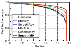
(a) $\sigma=0.25$

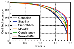
(b) $\sigma=0.50$

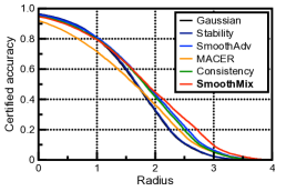
(c) $\sigma=1.00$

Figure 4: Comparison of approximate certified accuracy for various training methods on MNIST. The sharp drop of certified accuracy in each plot is due to that there is a strict upper bound in radius that Certify can output for a given $\sigma$ and $n=100,000$.

Table 3: Comparison of approximate certified test accuracy (%) and ACR on CIFAR-10. We set our results bold-faced whenever the value improves the Gaussian baseline, and underlined whenever the value improves the best among the considered baselines. ^∗ indicates that the results are evaluated from the official pre-trained models released by authors.

$\sigma$ Models (CIFAR-10) ACR 0.00 0.25 0.50 0.75 1.00 1.25 1.50 1.75 0.25 Gaussian [11] 0.424 76.6 61.2 42.2 25.1 0.0 0.0 0.0 0.0 Stability training [38] 0.421 72.3 58.0 43.3 27.3 0.0 0.0 0.0 0.0 SmoothAdv^∗ [49] 0.544 73.4 65.6 57.0 47.5 0.0 0.0 0.0 0.0 MACER^∗ [65] 0.531 79.5 69.0 55.8 40.6 0.0 0.0 0.0 0.0 Consistency [23] 0.552 75.8 67.6 58.1 46.7 0.0 0.0 0.0 0.0 SmoothMix (Ours) 0.553 77.1 67.9 57.9 46.7 0.0 0.0 0.0 0.0 + One-step adversary 0.548 74.2 66.1 57.4 47.7 0.0 0.0 0.0 0.0 0.50 Gaussian [11] 0.525 65.7 54.9 42.8 32.5 22.0 14.1 8.3 3.9 Stability training [38] 0.521 60.6 51.5 41.4 32.5 23.9 15.3 9.6 5.0 SmoothAdv^∗ [49] 0.684 65.3 57.8 49.9 41.7 33.7 26.0 19.5 12.9 MACER^∗ [65] 0.691 64.2 57.5 49.9 42.3 34.8 27.6 20.2 12.6 Consistency [23] 0.720 64.3 57.5 50.6 43.2 36.2 29.5 22.8 16.1 SmoothMix (Ours) 0.715 65.0 56.7 49.2 41.2 34.5 29.6 23.5 18.1 + One-step adversary 0.737 61.8 55.9 49.5 43.3 37.2 31.7 25.7 19.8

4.1 Results on MNIST

For MNIST [32] experiments, we report the approximate certified accuracy and ACR of smoothed classifiers obtained from LeNet [32] with different training methods, including SmoothMix, using the full MNIST test dataset. We consider three different models as varying the noise level $\sigma\in\{0.25,0.5,1.0\}$. During inference, we apply randomized smoothing with the same $\sigma$ used in the training. When SmoothMix is used, we consider a fixed hyperparameter value for $\alpha=1.0$ and $m=4$, the step size and the number of noise samples. We empirically observe that it is beneficial to set $\alpha\cdot T$ to be proportional to $\sigma$, the noise level, as there exist different upper bounds on the certified radius statistical achievable in practice depending on $\sigma$: in this respect, we set $T=2,4,8$ for the models with $\sigma=0.25,0.5,1.0$, respectively. We apply the same $m=4$ for SmoothAdv, i.e., for adversarial training, as well, and $T=10$ with an $\ell_{2}$-constraint of radius $\varepsilon=1.0$. Here, notice that SmoothMix and SmoothAdv use the same number of hyperparameters: more specifically, although SmoothMix introduces $\alpha$ compared to SmoothAdv, the step size in (8), it instead does not use the hyperparameter $\varepsilon$ of SmoothAdv, i.e., the maximum norm of adversarial perturbations.

The results are presented in Table 2 and Figure 4. Overall, we observe that our proposed SmoothMix loss (10) added to the Gaussian training dramatically improves the certified test accuracy from “Gaussian”. By considering the one-step adversary (Section 3.2) in training, we could further improve the robust accuracy, significantly improving ACRs compared to the previous state-of-the-art training methods: e.g., our method could improve ACRs with $\sigma=1.0$ from $1.779\rightarrow 1.823$. This shows that improvements from SmoothMix can be orthogonal to those from SmoothAdv. It is also remarkable that even without the one-step adversarial example, one could further improve the certified robustness by simply increasing the relative strength $\eta$ of the SmoothMix loss, e.g., by $1.0\rightarrow 5.0$ as presented in Table 2: e.g., “SmoothMix” with $\eta=5.0$ still outperforms “SmoothAdv” by $1.779\rightarrow 1.820$ at $\sigma=1.0$. Finally, we note that our models could substantially improve the robustness at larger perturbations with less degradation in the clean accuracy, e.g., compared to “MACER” or “Consistency”: considering that they are also regularization based approaches that allow to control the robustness via controlling their regularization strength, the results show that our form of loss could better compensate the trade-off between accuracy and robustness.

4.2 Results on CIFAR-10

For CIFAR-10 [29] experiments, we report the approximate certified accuracy and ACR of smoothed classifiers from ResNet-110 [20] using the full CIFAR-10 test dataset. Again, we consider three different models as varying the noise level $\sigma\in\{0.25,0.5,1.0\}$, and apply the same $\sigma$ for inference as well. When SmoothMix is used, we consider a fixed hyperparameter value for $T=4$ and $m=2$, the number of steps and the number of noise samples, respectively. We also fix $\eta=5.0$ throughout the experiments, as also used for MNIST (see Table 2). Again, we make sure that $\alpha\cdot T$ to be proportional to $\sigma$, so that we set $\alpha=0.5,1.0,2.0$ for the models with $\sigma=0.25,0.5,1.0$, respectively. For SmoothAdv, we report the performance evaluated from the pre-trained models released by the authors for a fixed configuration of $T=10,\varepsilon=1.0$, and $m=8$.

The results are summarized in Table 3 and Figure 6. Again, we still observe that our method generally exhibits better trade-offs between accuracy and certified robustness compared to other baselines: e.g., at $\sigma=0.5$, “SmoothMix” could improve the previous best result from “Consistency” by a significant margin of $0.720\rightarrow 0.737$. Without the single-step adversary, “SmoothMix” can effectively preserve the clean accuracy while also improving ACR, e.g., at $\sigma=0.25$, “SmoothMix” could even improve the clean accuracy of “Gaussian”: although “MACER” could improve the clean accuray as well, one could see that their improvements in robust accuracy are relatively limited. It is also notable that the certified test accuracy we report in Table 3 can sometimes complement ACR: although “Consistecny” achieves a competitive ACR with “SmoothMix” at $\sigma=0.25$, one can still confirm the superiority of “SmoothMix” by comparing the certified accuracy $r=0.0$ (i.e., the clean accuracy), namely 75.8% vs. 77.1%, given that they both achieve similar certified accuracy at $r=0.75$ (i.e., the robust accuracy). This is because a bare increase in the clean accuracy (i.e., $\hat{f}$ correctly classifies more test samples but with $\mathrm{CR}$’s closer to 0) often contributes less to the increase in ACR.

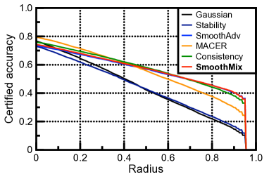
(a) $\sigma=0.25$

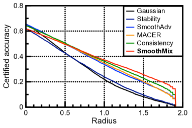
(b) $\sigma=0.50$

Figure 5: Comparison of approximate certified accuracy for various training methods on CIFAR-10. The sharp drop of certified accuracy in each plot is due to that there is a strict upper bound in radius that Certify can output for a given $\sigma$ and $n=100,000$.

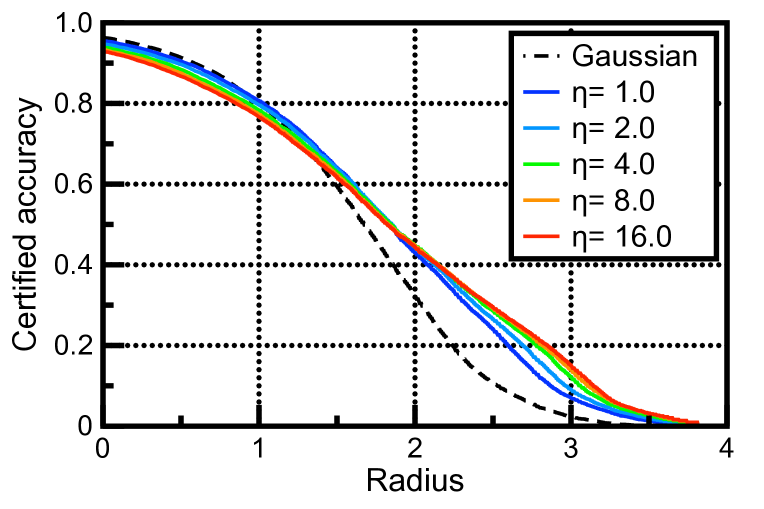
Figure 6: Comparison of approximate certified test accuracy of SmoothMix for varying $\eta$. “Gaussian” indicates the baseline training with Gaussian augmentation.

4.3 Ablation study

We also conduct an ablation study to investigate the individual effects of the hyperparameters in our method. Unless otherwise noted, we perform experiments on MNIST with $\sigma=1.0$. All the detailed results from this ablation study are reported in Appendix H.

Equal-confidence mixing ratios. Recall from Figure 3 that we are motivated by the problem of miscalibration in smoothed classifiers between clean and its adversarial example. To see how much the proposed SmoothMix could alleviate this issue, we compare the distributions of the minimal mixing ratios that changes its prediction of a given classifier on the CIFAR-10 test samples, namely the equal-confidence mixing ratios, before and after training with SmoothMix. We find the adversarial examples separately from two pre-trained ResNet-110 based (smoothed) classifiers, each trained by Gaussian training and SmoothMix, respectively, assuming $\sigma=0.25$. We optimize each adversarial example assuming only a quite loose norm-bound of $\varepsilon=8$ to allow more update steps, i.e., via 50-step PGD for both classifiers. Figure 3 shows the result, and it indeed confirms SmoothMix has an effect of improving calibration between clean and adversarial examples.

Effect of $\eta$. By design, SmoothMix controls the trade-off between accuracy and robustness by adjusting $\eta$, the relative strength of $L^{\tt mix}$ over $L^{\tt nat}$ (11). Here, we further examine the effect of $\eta$ by comparing the certified robustness on varying $\eta\in\{1,2,4,8,16\}$: the results in Figure 6 show that increasing $\eta$ consistently improves the certified robustness of the classifier, which confirms $L^{\tt mix}$, the mixup loss, as an effective term to trade-off the robustness against $L^{\tt nat}$ for accuracy.

Trade-off between $\alpha$ and $T$. In practice, SmoothMix can trade-off between the step size $\alpha$ and the number of steps $T$ to compensate between a more accurate optimization of (7) and its computational cost, while maintaining the effective range of the perturbation by $\alpha\cdot T$. Figure 7(a) explores this trade-off, by comparing models trained with different combinations of $(\alpha,T)$ under control of $\alpha\cdot T=8.0$. Interestingly, the results indicate that the choice of $\alpha$ and $T$ does not significantly affect the final performance as long as $\alpha\cdot T$ is constant: all the considered combinations achieve similar robustness, with only a slight degradation in ACR even at $(\alpha,T)=(8.0,1)$ (see Table 9 in Appendix H). This suggests that (a) finding adversarial examples in a smoothed classifier can be simpler than one might expect, and (b) one can effectively reduce the training cost of SmoothMix using small $T$ in practice.

Hard restriction on adversarial attacks. One of key features of SmoothMix is at its unrestricted search of adversarial examples. Here, we examine the case when there is a hard restriction on each search, namely in $\ell_{2}$-radius of $\varepsilon\in\{2,4,6,8\}$. The results presented in Figure 7(b) along with the Gaussian baseline (“Gaussian”) and the original unrestricted setup (“$\varepsilon=\infty$”) show that SmoothMix indeed works best when there is no such restrictions, although these ablations still reasonably improve the Gaussian baseline, i.e., calibrating with adversarial examples outside the $\varepsilon$-ball can indeed help to improve the certified robustness in our training scheme.

Effect of $m$. Figure 7(c) (and Table 11 in Appendix H) investigates the effect of using different $m\in\{1,2,4,8\}$, the number of noise samples to approximate the prediction of smoothed classifier: the larger $m$, the better approximation of smoothed classifier, which would be beneficial for both natural loss and SmoothMix loss (11). Overall, we observe that SmoothMix can still improve ACR from “Gaussian” even with $m=1$, but with a moderate degradation in the clean accuracy: as $m$ is one of the crucial factors related to the total training cost in practice, one is recommended to use smaller $m$, e.g., $m=2$ or $4$, considering its little effect to the final ACR.

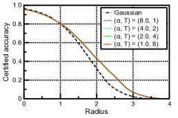
(a) Effect of $\alpha$ and $T$

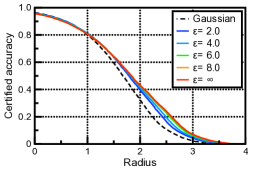
(b) Hard restriction of $\varepsilon$ on attacks

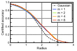
(c) Effect of $m$

Figure 7: Comparison of approximate certified test accuracy of SmoothMix and its ablations. “Gaussian” indicates the baseline training with Gaussian augmentation.

5 Discussion and conclusion

We observe that adversarial training with an unrestricted adversary can be feasible and even more promising (compared to the restricted ones) when it comes with smoothed classifiers, by showing their effectiveness to improve the certified adversarial robustness with a novel mixup-based training. We address the brittleness of deep neural networks through the lens of smoothed classifiers, which could give us a simpler view on them. We believe our research could be a useful step toward understanding what essentially constitutes adversarial examples in deep neural networks.

Broader impact. Adversarial robustness in deep learning is arguably an essential requirement for AI safety [2], with much impact on various security-concerned systems: e.g., medical diagnosis [9], speech recognition [46] and autonomous driving [64]. Thanks to their certifiable guarantees, we believe a practical success of systems based on randomized smoothing would be fatal for those who maliciously attempt to break down the system via adversarial attacks. Nevertheless, one should also recognize that current techniques for robustness in deep learning, including randomized smoothing as well, indeed have a clear gap to be practically used in real-world, e.g., defending against challenging unrestricted attacks [60, 5], which should be further investigated in the future research. Consequently, it is particularly important for the defense techniques not to be misused in practical systems, as a failure of such systems may lead practitioners to have a biased, false sense of security.

Limitation. While our ultimate goal is to find optimal smoothed classifiers in terms of the accuracy and robustness trade-off, SmoothMix should not be considered as the final solution for the problem; our method is a promising proof-of-concept showing the close relationship between randomized smoothing and confidence-calibrated classifiers [19, 36]. Although our focus in this paper is currently limited only to the over-confidence issue, we believe there are still many rooms to be explored in future for another such connection, e.g., could the recent developments in the literature of uncertainty estimation of deep neural networks [22, 54] help to improve the robustness of smoothed classifiers.

Appendix A Training procedure of SmoothMix

Algorithm 1 SmoothMix training

0:  Sample $(x,y)\sim P$. smoothing factor $\sigma$. number of noise samples $m$. number of steps $T$. step size $\alpha$. regularization strength $\eta>0$.  

1:  Sample $\delta_{1},\cdots,\delta_{m}\sim\mathcal{N}(0,\sigma^{2}I)$, and $\lambda\sim\mathcal{U}(\left[0,\tfrac{1}{2}\right])$

2:  // Find an adversarial example

3:  $\tilde{x}^{(0)},\hat{F}(x^{(0)})\leftarrow x,\frac{1}{m}\sum_{i=1}^{m}F(x+\delta_{i})$

4:  for $t=0$ to $T-1$ do

5:     $J(\tilde{x}^{(t)})\leftarrow-\log\hat{F}_{y}(\tilde{x}^{(t)})$

6:     $\tilde{x}^{(t+1)}\leftarrow\tilde{x}^{(t)}+\alpha\cdot\frac{\nabla_{x}J(\tilde{x}^{(t)})}{\|\nabla_{x}J(\tilde{x}^{(t)})\|_{2}}$

7:     $\hat{F}(\tilde{x}^{(t+1)})\leftarrow\frac{1}{m}\sum_{i=1}^{m}F(\tilde{x}^{(t+1)}+\delta_{i})$

8:  end for

9:  if $~{}\mathtt{use\_single\_step}~{}$ then $~{}x\leftarrow\tilde{x}^{(1)}~{}$

10:  // Compute the SmoothMix loss

11:  $x^{\tt mix},y^{\tt mix}\leftarrow((1-\lambda)\cdot x+\lambda\cdot\tilde{x}^{(T)}),((1-\lambda)\cdot\hat{F}(x)+\lambda\cdot\tfrac{\mathbbm{1}}{C})$

12:  for $i=1$ to $m$ do

13:     $L^{\tt nat}_{i},L^{\tt mix}_{i}\leftarrow\mathcal{L}(F(x+\delta_{i}),y),\mathcal{L}(F(x^{\tt mix}+\delta_{i}),y^{\tt mix})$

14:  end for

15:  $L\leftarrow\frac{1}{m}\sum_{i}(L^{\tt nat}_{i}+\eta\cdot L^{\tt mix}_{i})$

Appendix B Discussion on input-dependent designs of noise scales

In this paper, we aim to develop a new training method to exhibit a better trade-off between accuracy and (certified) robustness of smoothed classifiers. Meanwhile, there has been recently another proposal to improve the robustness of smoothed classifiers without a new training scheme, namely by certifying a given smoothed classifier with input-dependent $\sigma$ [1, 58, 10]. In this section, however, we show that if one allows different noise scales $\sigma$ for each input in attempt to generalize the current framework of randomized smoothing [11], then the actual robustness guarantee would rapidly decrease as the input dimension grows. In particular, we consider the following classifier $\tilde{f}$ generalizing (2) with some non-negative function $g:\mathbb{R}^{d}\rightarrow\mathbb{R}_{\geq 0}$, defined as follows:

$$\tilde{f}(x):=\operatorname*{arg\,max}_{c\in\mathcal{Y}}\mathbb{P}_{\delta\sim\mathcal{N}(0,g(x)I)}(f(x+\delta)=c),$$

In other words, we assume that the scaling parameter of the smoothing noise can now be a function of $x$. As in the main text, we are interested in the certified radius $\underline{R}(\tilde{f};x,y)$ of $\tilde{f}$.

One may expect that $\underline{R}(\tilde{f};x,y)$ can be significantly larger than $\underline{R}(\hat{f};x,y)$ since $\hat{f}$ is a special case of $\tilde{f}$, i.e., constant $g(x)$. However, we show that it may not be true for high-dimensional inputs: even a small deviation of $g(x)$ can incur very poor certified robustness. Formally, we prove the following theorem.

Theorem 1.

Let $r_{i},i\in\mathbb{N}$ be any i.i.d. random variables of zero mean, unit variance, and $\mathbb{E}[r_{i}^{4}]<\infty$. Let $\mathcal{F}_{d}$ be a collection of all measurable functions from $\mathbb{R}^{d}$ to $\{0,1\}$. Let $p\in(0.5,1)$, $\sigma,\tau>0$, and $\varepsilon\in(0,1/2]$ be constants such that $\sigma\neq\tau$. Then, for $\delta:=(r_{1},\dots,r_{d})$, for any $c\in\{0,1\}$, and for any $d\in\mathbb{N}$, the following statements hold:

$$\sup_{x,x^{\prime}\in\mathbb{R}^{d}:\|x-x^{\prime}\|_{2}\leq\varepsilon}\inf_{f\in\mathcal{F}_{d}:\mathbb{P}(f(x+\sigma\delta)=c)=p}\mathbb{P}(f(x^{\prime}+\tau\delta)=c)\leq C/d.$$

for some constant $C>0$ which is a function of other constants $p,\sigma,\tau,\varepsilon,\mathbb{E}[r_{i}^{4}]$.

Theorem 1 indicates the curse of dimensionality for the worst classifier under general noises of a finite kurtosis. In particular, it states that there exists an upper bound on $\mathbb{P}(f(x+\tau\delta)=c)$ inversely proportional to the input dimension $d$ even though two inputs $x,x^{\prime}$ are extremely close. Hence, if we utilize different noise scales (i.e., $\sigma$) for each input, the resulting lower bound on the certified radius relying on the worst-case bound as in [11, 33, 49] will be small for high-dimensional inputs. Namely, choosing (almost) constant noise scale for the inputs in the target certification region is necessary.

B.1 Proof of Theorem 1

We first define $z=(z_{1},\dots,z_{d}):=x^{\prime}-x$, i.e., $\|z\|_{2}\leq\varepsilon$. Then, the following inequality trivially holds.

$$\inf_{f\in\mathcal{F}_{d}:\mathbb{E}[f(x+\sigma\delta)]=p}\mathbb{E}[f(x^{\prime}+\tau\delta)] \leq\inf_{\mathcal{U}\subset\mathbb{R}^{d}:\mathbb{P}(\sigma\delta\in\mathcal{U})=p}\mathbb{P}\left(\tau\delta+z\in\mathcal{U}\right)$$

$$\leq\mathbb{P}\left(\frac{\|\tau\delta+z\|_{2}^{2}}{d}\in[\sigma^{2}-k,\sigma^{2}+k]\right)$$ (12)

where $k$ is a non-negative number satisfying

$$\mathbb{P}\left(\frac{\|\sigma\delta\|_{2}^{2}}{d}\in[\sigma^{2}-k,\sigma^{2}+k]\right)=p.$$

The following lemma asserts that the RHS of (12) is bounded by $C/d$ where $C$ is some constant which is only a function of $\mathbb{E}[r_{i}^{4}],\sigma,\tau,\varepsilon,p$. This completes the proof of Theorem 1.

Lemma 2.

There exists $C$ which is a function of $\mathbb{E}[r_{i}^{4}],\sigma,\tau,\varepsilon,p$ such that the following statements hold: for any $d\in\mathbb{N}$ and for any $z\in\mathbb{R}^{d}$ satisfying $\|z\|_{2}\leq\varepsilon$,

$$\mathbb{P}\left(\frac{\|\tau\delta+z\|_{2}^{2}}{d}\in[\sigma^{2}-k,\sigma^{2}+k]\right)\leq\frac{C}{d}.$$

B.2 Proof of Lemma 2

Lemma 2 is a direct consequence of the law of large numbers applied to the i.i.d. random variables $r_{i}^{2}$. First, we compute the variance of $\frac{\|\sigma\delta\|_{2}^{2}}{d}$ using the following equality: for $\eta:=\sqrt{\mathbb{E}[r_{i}^{4}]-1}$,

$$\text{Var}\left(\frac{\|\sigma\delta\|_{2}^{2}}{d}\right) =\mathbb{E}\left[\left(\frac{\|\sigma\delta\|_{2}^{2}}{d}-\sigma^{2}\right)^{2}\right]=\mathbb{E}\left[\left(\frac{\sigma^{2}}{d}\sum_{i=1}^{d}(r_{i}^{2}-1)\right)^{2}\right]$$

$$=\frac{\sigma^{4}}{d^{2}}\sum_{i=1}^{d}\mathbb{E}\left[(r_{i}^{2}-1)^{2}\right]=\frac{\sigma^{4}}{d^{2}}\sum_{i=1}^{d}\mathbb{E}[r_{i}^{4}]-1$$

$$=\frac{\sigma^{4}(\mathbb{E}[r_{i}^{4}]-1)}{d}=\frac{\sigma^{4}\eta^{2}}{d}$$

where the third equality follows from the independence of $r_{i}$s and the fourth inequality follows from $\mathbb{E}[r_{i}^{2}]=1$. Hence, from the Chebyshev’s inequality, we have

$$\mathbb{P}\left(\left|\frac{\|\sigma\delta\|_{2}^{2}}{d}-\sigma^{2}\right|<\frac{\sigma^{2}\eta}{\sqrt{d(1-p)}}\right)\geq 1-(\sqrt{1-p})^{2}=p,$$ (13)

i.e., $k\leq\frac{\sigma^{2}\eta}{\sqrt{d(1-p)}}$.

Now, we derive a similar concentration inequality for $\frac{\|\tau\delta+z\|_{2}^{2}}{d}$. To this end, we bound its deviation from $\tau^{2}+\frac{\|z\|_{2}^{2}}{d}$ as follows:

$$\mathbb{P}\left(\left|\frac{\|\tau\delta+z\|_{2}^{2}}{d}-\left(\tau^{2}+\frac{\|z\|_{2}^{2}}{d}\right)\right|\geq\frac{\sigma^{2}+\tau^{2}}{3}\right)$$

$$=1-\mathbb{P}\left(\left|\frac{\|\tau\delta+z\|_{2}^{2}}{d}-\left(\tau^{2}+\frac{\|z\|_{2}^{2}}{d}\right)\right|<\frac{\sigma^{2}+\tau^{2}}{3}\right)$$

$$\leq 1-\mathbb{P}\left(\left|\frac{\|\tau\delta\|_{2}^{2}}{d}-\tau^{2}\right|<\frac{\sigma^{2}+\tau^{2}}{6}\quad\text{and}\quad\left|\frac{2\tau\sum_{i=1}^{d}r_{i}z_{i}}{d}\right|<\frac{\sigma^{2}+\tau^{2}}{6}\right)$$

$$=\mathbb{P}\left(\left|\frac{\|\tau\delta\|_{2}^{2}}{d}-\tau^{2}\right|\geq\frac{\sigma^{2}+\tau^{2}}{6}\quad\text{or}\quad\left|\frac{2\tau\sum_{i=1}^{d}r_{i}z_{i}}{d}\right|\geq\frac{\sigma^{2}+\tau^{2}}{6}\right)$$

$$\leq\mathbb{P}\left(\left|\frac{\|\tau\delta\|_{2}^{2}}{d}-\tau^{2}\right|\geq\frac{\sigma^{2}+\tau^{2}}{6}\right)+\mathbb{P}\left(\left|\frac{2\tau\sum_{i=1}^{d}r_{i}z_{i}}{d}\right|\geq\frac{\sigma^{2}+\tau^{2}}{6}\right)$$

$$\leq\frac{36\tau^{4}\eta^{2}+144\tau^{2}\varepsilon^{2}}{(\sigma^{2}+\tau^{2})^{2}d}$$ (14)

where the last inequality is from the variance bounds

$$\text{Var}\left(\frac{\|\tau\delta\|_{2}^{2}}{d}-\tau^{2}\right)=\frac{\tau^{4}\eta^{2}}{d}$$

$$\text{Var}\left(\frac{2\tau\sum_{i=1}^{d}r_{i}z_{i}}{d}\right)=\frac{4\tau^{2}\|z\|_{2}^{2}}{d^{2}}\leq\frac{4\tau^{2}\varepsilon^{2}}{d^{2}}$$

and the Chebyshev’s inequality

$$\mathbb{P}\left(\left|\frac{\|\tau\delta\|_{2}^{2}}{d}-\tau^{2}\right|\geq\frac{\sigma^{2}+\tau^{2}}{6}\right)\leq\frac{36\tau^{4}\eta^{2}}{(\sigma^{2}+\tau^{2})^{2}d}$$

$$\mathbb{P}\left(\left|\frac{2\tau\sum_{i=1}^{d}r_{i}z_{i}}{d}\right|\geq\frac{\sigma^{2}+\tau^{2}}{6}\right)\leq\frac{144\tau^{2}\varepsilon^{2}}{(\sigma^{2}+\tau^{2})^{2}d^{2}}.$$

Then, for all $d\geq\max\left\{\frac{4\sigma^{4}\eta^{2}}{(\tau^{2}-\sigma^{2})^{2}(1-p)},\frac{6\varepsilon^{2}}{\sigma^{2}+\tau^{2}}\right\}$, i.e., $\frac{\sigma^{2}\eta}{\sqrt{d(1-p)}}\leq\frac{|\tau^{2}-\sigma^{2}|}{2}$ and $\frac{\varepsilon^{2}}{d}\leq\frac{\sigma^{2}+\tau^{2}}{6}$, it holds that

$$\mathbb{P}\left(\frac{\|\tau\delta+z\|_{2}^{2}}{d}\in[\sigma^{2}-k,\sigma^{2}+k]\right)$$

$$\leq\mathbb{P}\left(\frac{\|\tau\delta+z\|_{2}^{2}}{d}\in\left[\sigma^{2}-\frac{|\tau^{2}-\sigma^{2}|}{2},\sigma^{2}+\frac{|\tau^{2}-\sigma^{2}|}{2}\right]\right)$$

$$\leq\mathbb{P}\left(\left|\frac{\|\tau\delta+z\|_{2}^{2}}{d}-\left(\tau^{2}+\frac{\|z\|_{2}^{2}}{d}\right)\right|\geq\frac{\sigma^{2}+\tau^{2}}{3}\right)$$

$$\leq\frac{36\tau^{4}\eta^{2}+144\tau^{2}\varepsilon^{2}}{(\sigma^{2}+\tau^{2})^{2}d}$$

by using (14). Hence, choosing

$$C:=\max\left\{\frac{4\sigma^{4}\eta^{2}}{(\tau^{2}-\sigma^{2})^{2}(1-p)},\frac{6\varepsilon^{2}}{\sigma^{2}+\tau^{2}},\frac{36\tau^{4}\eta^{2}+144\tau^{2}\varepsilon^{2}}{(\sigma^{2}+\tau^{2})^{2}}\right\}$$

completes the proof of Lemma 2.

Appendix C Experimental details

Throughout our experiments, we follow the same training details of prior works [11, 49, 65, 23] for a fair comparison: more specifically, we use LeNet [32] for MNIST, ResNet-110 [20] for CIFAR-10, and ResNet-50 [20] for ImageNet. We train every model via stochastic gradient descent using Nesterov momentum of weight 0.9 without dampening. We set a weight decay of $10^{-4}$ for all the models. We consider three different noise levels $\sigma\in\{0.25,0.5,1.0\}$ for smoothing classifiers for MNIST and CIFAR-10 models, and $\sigma\in\{0.5,1.0\}$ in the case of ImageNet. We used up to 4 NVIDIA TITAN Xp GPUs to run each configurations considered in our experiments, both for training and certification: more specifically, we used a single GPU to run every experimenet on MNIST and CIFAR-10, and four GPUs to run ImageNet models.

C.1 Datasets

MNIST dataset [32] consists 70,000 gray-scale hand-written digit images of size 28$\times$28, 60,000 for training and 10,000 for testing. Each of the images is labeled from 0 to 9, i.e., there are 10 classes. We do not perform any pre-processing except for normalizing the range of each pixel from 0-255 to 0-1. When MNIST is used for training, we use LeNet [32] for 90 epochs and use the initial learning rate of 0.01. The learning rate is decayed by 0.1 at 30-th and 60-th epoch.

CIFAR-10 dataset [29] consist of 60,000 RGB images of size 32$\times$32 pixels, 50,000 for training and 10,000 for testing. Each of the images is labeled to one of 10 classes, and the number of data per class is set evenly, i.e., 6,000 images per each class. We use the standard data-augmentation scheme of random horizontal flip and random translation up to 4 pixels, as also used by other baselines [11, 49, 65, 23]. We also normalize the images in pixel-wise by the mean and the standard deviation calculated from the training set. When CIFAR-10 is used for training, we train ResNet-110 [20] models for 150 epochs with initial learning rate of 0.1. The learning rate if decated by 0.1 at 50-th and 100-th epoch.

ImageNet classification dataset [48] consists of 1.2 million training images and 50,000 validation images, which are labeled by one of 1,000 classes. For data-augmentation, we perform 224$\times$224 random cropping with random resizing and horizontal flipping to the training images. At test time, on the other hand, 224$\times$224 center cropping is performed after re-scaling the images into 256$\times$256. When ImageNet is used for training, we train ResNet-50 [20] models for 90 epochs with initial learning rate of 0.1. The learning rate if decated by 0.1 at 30-th and 60-th epoch.

C.2 Detailed hyperparameters for baselines

Stability training [38] uses a single hyperparameter $\lambda>0$ to control the relative strength of the stability regularization compared to the standard cross-entropy loss. In our experiments, we use $\lambda=2$ by default for this method, but except for the “$\sigma=1.0$” model on CIFAR-10: in this case, we had to reduce it to $\lambda=1$ for a stable training.

SmoothAdv [49] mainly controls three hyperparameters those are for performing projected gradient descent (PGD) to find adversarial examples in the training: namely, it uses $m$: the number of noise samples, $T$: the number of PGD steps, and $\varepsilon$: an $\ell_{2}$-norm restriction on adversarial perturbations. For SmoothAdv models, we fix $T=10$ and $\varepsilon=1.0$ throughout the experiments. In case of $m$, and use $m=4$ for MNIST models, and $m=8$ for CIFAR-10. Following Salman et al. [49], we also adopt the warm-up strategy on $\varepsilon$, i.e., it is initially set to zero, and gradually increased for the first 10 epochs up to the original value of $\varepsilon$.

MACER [65] adds four hyperparameters to the training: namely, it uses $m$: the number of noise samples, $\lambda$: the relative strength of regularization, $\beta$: a temperature scaling factor, and $\gamma$: a margin gap. We follow the configurations reported by Zhai et al. [65] to reproduce the MNIST results: namely, we use $m=16$, $\beta=16.0$, $\gamma=8.0$ and $\lambda=16.0$. We use $\lambda=6.0$ in case of $\sigma=1.0$ on MNIST, however, for a better training stability. We use the pre-trained models released by the authors for evaluations on CIFAR-10, which can be downloaded at https://github.com/RuntianZ/macer. These CIFAR-10 models are reported to be trained with $m=16$, $\beta=16.0$, $\gamma=8.0$, and $\lambda=12.0$ and $4.0$ for $\sigma=0.25$ and $0.5$, respectively. For $\sigma=1.0$, $\lambda$ is initially set to 0, and changed to $\lambda=12.0$ after the first learning rate decay.

Consistency [23] controls two hyperparameters, namely $\lambda$ and $\eta$, each for the relative strength of the consistency term and the entropy term, respectively. We obtain results from the best hyperparameters those reported by Jeong and Shin [23] when the consistency regularization is applied to the Gaussian training baseline, both in MNIST and CIFAR-10 datasets. More concretely, we fix $\eta=0.5$ for every model, and use $\lambda=5$ for MNIST and $\lambda=10$ for CIFAR-10 models by default. In case of $\sigma=0.25$, $\lambda$ is doubled in both datasets, i.e., $\lambda=10$ and $\lambda=20$ for MNIST and CIFAR-10, respectively, as it is shown to achieve better ACRs.

Appendix D Related work

Certified adversarial robustness. We focus on improving adversarial robustness of randomized smoothing [11] based classifiers, which is currently one of prominent ways to obtain a classifier with a robustness certification. In general, there have been many attempts other than randomized smoothing to provide a robustness certification of deep neural networks [16, 59, 42, 61, 18, 68], and correspondingly with attempts to further improve the robustness with respect to those certification protocols [13, 12, 4]. Nevertheless, randomized smoothing has attracted particular attention as the first approach that could successfully scaled up to the ImageNet dataset [48]. A more complete taxonomy on the literature can be found in Li et al. [39].

Confidence-calibrated training. Overconfident predictions of deep neural networks [45] have been considered as problematic in many scenarios, e.g., uncertainty estimation of in-distribution samples [19, 24, 30], those of out-of-distribution samples [21, 36, 41], and ensemble learning [35], just to name a few. In the context of adversarial training, Stutz et al. [52] have shown that regularizing confidence on adversarial examples to be uniform can improve detection of adversarial examples from unseen threat models. In this paper, we address the overconfidence at adversarial examples particularly focusing on smoothed classifiers, observing that a simple approach of directly fixing the problem could significantly improve the certified robustness.

Mixup-based training. Originally, mixup [67] has proposed as a simple yet effective data augmentation scheme to improve generalization and robustness (against small adversarial attacks) of deep neural networks, and there have been significant follow-up works to further improve this form [57, 63, 27, 28]. Recently, Zhang et al. [70] have also explored on theoretical justifications behind how could such an augmentation improves generalization and robustness. Although our method uses a similar linear interpolation scheme of mixup, there is still an essential difference between ours and this line of works: namely, we do not rely on the prior of interpolating two (or more) independent samples, but rather aims to directly calibrate predictions between a clean and its (unrestricted) adversarial example, i.e., we consider a new form of self-mixup training.

There have been also attempts to employ mixup particularly for improving adversarial robustness: Lamb et al. [31] have shown that an additional mixup loss between adversarial examples upon the standard mixup training achieves a comparable robustness to adversarial training (AT) [40], while not compromising the clean accuracy as much as AT; Lee et al. [37] have proposed Adversarial Vertex Mixup to improve AT, by extrapolating predictions along the direction of adversarial perturbation up to few times of its norm via mixup training. Our proposed method can be differentiated to these approaches, in a sense that we employ mixup not to directly improve the robustness of a given neural network, but of its smoothed counterpart. It is also our unique perspective that we consider unrestricted adversarial examples to be interpolated.

Appendix E Variance of results over multiple runs

In our experiments, we report single-run results for ACR and certified robust accuracy as also done by [11, 49, 38, 65, 23], considering that ACR is fairly a robust metric to network initialization: e.g., in Table 5, we report the mean and standard deviation of ACRs across 5 seeds for the MNIST results reported in Table 2. Overall, we confirm that ACR generally shows low variance over multiple runs across a wide range of training methods, including ours.

Table 4: Comparison of certified test accuracy for various training methods on MNIST. The reported values are the mean and standard deviation across 5 seeds. We set our result bold-faced whenever the value improves the Gaussian baseline, and the underlined are best-performing model per $\sigma$.

$\sigma$ Models (MNIST) 0.00 0.50 1.00 1.50 2.00 2.50 0.25 Gaussian [11] 99.25 $\pm$ 0.04 96.75 $\pm$ 0.11 0.00 $\pm$ 0.00 0.00 $\pm$ 0.00 0.00 $\pm$ 0.00 0.00 $\pm$ 0.00 Stability training [38] 99.34 $\pm$ 0.04 97.12 $\pm$ 0.12 0.00 $\pm$ 0.00 0.00 $\pm$ 0.00 0.00 $\pm$ 0.00 0.00 $\pm$ 0.00 SmoothAdv [49] 99.39 $\pm$ 0.01 98.17 $\pm$ 0.06 0.00 $\pm$ 0.00 0.00 $\pm$ 0.00 0.00 $\pm$ 0.00 0.00 $\pm$ 0.00 MACER [65] 99.33 $\pm$ 0.03 97.35 $\pm$ 0.08 0.00 $\pm$ 0.00 0.00 $\pm$ 0.00 0.00 $\pm$ 0.00 0.00 $\pm$ 0.00 Consistency [23] 99.43 $\pm$ 0.03 97.92 $\pm$ 0.09 0.00 $\pm$ 0.00 0.00 $\pm$ 0.00 0.00 $\pm$ 0.00 0.00 $\pm$ 0.00 SmoothMix ($\eta$ = 1.0) 99.43 $\pm$ 0.03 98.10 $\pm$ 0.06 0.00 $\pm$ 0.00 0.00 $\pm$ 0.00 0.00 $\pm$ 0.00 0.00 $\pm$ 0.00 + One-Step adversary 99.39 $\pm$ 0.02 98.17 $\pm$ 0.06 0.00 $\pm$ 0.00 0.00 $\pm$ 0.00 0.00 $\pm$ 0.00 0.00 $\pm$ 0.00 SmoothMix ($\eta$ = 5.0) 99.45 $\pm$ 0.03 98.17 $\pm$ 0.07 0.00 $\pm$ 0.00 0.00 $\pm$ 0.00 0.00 $\pm$ 0.00 0.00 $\pm$ 0.00 + One-Step adversary 99.37 $\pm$ 0.02 98.20 $\pm$ 0.03 0.00 $\pm$ 0.00 0.00 $\pm$ 0.00 0.00 $\pm$ 0.00 0.00 $\pm$ 0.00 0.50 Gaussian [11] 99.15 $\pm$ 0.03 96.90 $\pm$ 0.06 89.83 $\pm$ 0.06 67.80 $\pm$ 0.16 0.00 $\pm$ 0.00 0.00 $\pm$ 0.00 Stability training [38] 99.26 $\pm$ 0.02 97.27 $\pm$ 0.09 90.75 $\pm$ 0.11 69.15 $\pm$ 0.38 0.00 $\pm$ 0.00 0.00 $\pm$ 0.00 SmoothAdv [49] 99.03 $\pm$ 0.03 97.36 $\pm$ 0.06 92.94 $\pm$ 0.08 81.06 $\pm$ 0.12 0.00 $\pm$ 0.00 0.00 $\pm$ 0.00 MACER [65] 98.69 $\pm$ 0.09 96.28 $\pm$ 0.17 90.14 $\pm$ 0.20 72.12 $\pm$ 0.75 0.00 $\pm$ 0.00 0.00 $\pm$ 0.00 Consistency [23] 99.15 $\pm$ 0.03 97.51 $\pm$ 0.07 92.89 $\pm$ 0.10 78.26 $\pm$ 0.23 0.00 $\pm$ 0.00 0.00 $\pm$ 0.00 SmoothMix ($\eta$ = 1.0) 99.10 $\pm$ 0.02 97.51 $\pm$ 0.07 92.91 $\pm$ 0.08 80.15 $\pm$ 0.05 0.00 $\pm$ 0.00 0.00 $\pm$ 0.00 + One-Step adversary 98.74 $\pm$ 0.04 97.09 $\pm$ 0.06 92.67 $\pm$ 0.05 81.70 $\pm$ 0.05 0.00 $\pm$ 0.00 0.00 $\pm$ 0.00 SmoothMix ($\eta$ = 5.0) 98.64 $\pm$ 0.04 96.98 $\pm$ 0.02 92.63 $\pm$ 0.07 81.85 $\pm$ 0.10 0.00 $\pm$ 0.00 0.00 $\pm$ 0.00 + One-Step adversary 98.21 $\pm$ 0.02 96.34 $\pm$ 0.04 91.46 $\pm$ 0.03 81.20 $\pm$ 0.15 0.00 $\pm$ 0.00 0.00 $\pm$ 0.00 1.00 Gaussian [11] 96.34 $\pm$ 0.03 91.39 $\pm$ 0.05 79.86 $\pm$ 0.08 59.49 $\pm$ 0.10 32.46 $\pm$ 0.20 10.93 $\pm$ 0.12 Stability training [38] 96.43 $\pm$ 0.05 91.63 $\pm$ 0.05 80.45 $\pm$ 0.16 60.53 $\pm$ 0.07 33.35 $\pm$ 0.13 11.05 $\pm$ 0.13 SmoothAdv [49] 95.76 $\pm$ 0.03 90.72 $\pm$ 0.07 80.81 $\pm$ 0.14 64.44 $\pm$ 0.14 43.25 $\pm$ 0.14 22.58 $\pm$ 0.40 MACER [65] 91.59 $\pm$ 0.20 83.44 $\pm$ 0.35 71.10 $\pm$ 0.45 55.67 $\pm$ 0.27 38.67 $\pm$ 0.33 20.09 $\pm$ 0.64 Consistency [23] 94.96 $\pm$ 0.02 89.75 $\pm$ 0.07 79.70 $\pm$ 0.09 63.54 $\pm$ 0.12 41.74 $\pm$ 0.13 20.22 $\pm$ 0.25 SmoothMix ($\eta$ = 1.0) 95.52 $\pm$ 0.08 90.50 $\pm$ 0.07 80.55 $\pm$ 0.09 64.09 $\pm$ 0.15 43.16 $\pm$ 0.05 23.94 $\pm$ 0.19 + One-Step adversary 94.72 $\pm$ 0.07 89.40 $\pm$ 0.09 79.46 $\pm$ 0.08 64.04 $\pm$ 0.08 44.82 $\pm$ 0.09 27.35 $\pm$ 0.15 SmoothMix ($\eta$ = 5.0) 93.71 $\pm$ 0.04 88.00 $\pm$ 0.05 77.95 $\pm$ 0.13 62.78 $\pm$ 0.08 44.87 $\pm$ 0.14 28.88 $\pm$ 0.16 + One-Step adversary 93.11 $\pm$ 0.05 87.24 $\pm$ 0.07 77.22 $\pm$ 0.10 62.48 $\pm$ 0.15 44.85 $\pm$ 0.05 29.66 $\pm$ 0.15

Table 5: Comparison of ACR for various training methods on MNIST. The reported values are the mean and standard deviation across 5 seeds. We set our result bold-faced whenever the value improves the Gaussian baseline, and the underlined are best-performing model per $\sigma$.

ACR (MNIST)	$\sigma=0.25$	$\sigma=0.50$	$\sigma=1.00$
Gaussian [11]	0.9108$\pm$0.0003	1.5581$\pm$0.0016	1.6184$\pm$0.0021
Stability [38]	0.9152$\pm$0.0007	1.5719$\pm$0.0028	1.6341$\pm$0.0018
SmoothAdv [49]	0.9322$\pm$0.0005	1.6872$\pm$0.0007	1.7786$\pm$0.0017
MACER [65]	0.9201$\pm$0.0006	1.5899$\pm$0.0069	1.5950$\pm$0.0051
Consistency [23]	0.9279$\pm$0.0003	1.6549$\pm$0.0011	1.7376$\pm$0.0017
SmoothMix ($\eta=1.0$)	0.9296$\pm$0.0003	1.6776$\pm$0.0007	1.7867$\pm$0.0020
+ One-Step adversary	0.9330$\pm$0.0004	1.6932$\pm$0.0009	1.8169$\pm$0.0011
SmoothMix ($\eta=5.0$)	0.9317$\pm$0.0002	1.6932$\pm$0.0007	1.8185$\pm$0.0016
+ One-Step adversary	0.9332$\pm$0.0002	1.6851$\pm$0.0003	1.8212$\pm$0.0013

Appendix F Additional results on CIFAR-10

In this section, we report additional experimental results on CIFAR-10 [29], namely with $\sigma=1.0$ (see Table 3 for the results for $\sigma\in\{0.25,0.5\}$). We follow the same experimental details as specified in Section 4.2 and Appendix C, including the common hyperparameter choice of $\eta=5.0$ for SmoothMix for other experiments as well. Again, we compare our method with various existing robust training methods for smoothed classifiers [11, 38, 49, 65, 23], and Table 6 summarizes the results. Overall, we still observe a similar trend to Section 4.2 that (a) “SmoothMix” offers a significant improvement of robust accuracy without compromising the clean accuracy much, and (b) incorporating the one-step adversary thus can further complementarily boost ACR to outperform other state-of-the-art baseline training methods: e.g., it is notable that “SmoothMix + One-step adversary” achieves fairly comparable or better robust accuracy than MACER while maintaining much higher clean accuracy, i.e., the certified test accuracy at $r=0.0$, namely 41.4 $\rightarrow$ 45.1. This confirms that our proposed SmoothMix can offer a better trade-off between accuracy and certified robustness during training.

Table 6: Comparison of approximate certified test accuracy (%) and ACR on CIFAR-10. All the models are trained and evaluated with the same smoothing factor specified by $\sigma$. Each value except ACR indicates the fraction of test samples those have $\ell_{2}$ certified radius larger than the threshold specified at the top row. We set our results bold-faced whenever the value improves the Gaussian baseline, and underlined whenever the value achieves the best among the considered baselines. ^∗ indicates that the results are evaluated from the official pre-trained models released by authors.

$\sigma$ Models (CIFAR-10) ACR 0.00 0.25 0.50 0.75 1.00 1.25 1.50 1.75 2.00 2.25 1.00 Gaussian [11] 0.542 47.2 39.2 34.0 27.8 21.6 17.4 14.0 11.8 10.0 7.6 Stability training [38] 0.526 43.5 38.9 32.8 27.0 23.1 19.1 15.4 11.3 7.8 5.7 SmoothAdv^∗ [49] 0.660 50.8 44.9 39.0 33.6 28.5 23.7 19.4 15.4 12.0 8.7 MACER^∗ [65] 0.744 41.4 38.5 35.2 32.3 29.3 26.4 23.4 20.2 17.4 14.5 Consistency [23] 0.756 46.3 42.2 38.1 34.3 30.0 26.3 22.9 19.7 16.6 13.8 SmoothMix (Ours) 0.725 47.1 42.5 37.5 32.9 28.7 24.9 21.3 18.3 15.5 12.6 + One-step adversary 0.773 45.1 41.5 37.5 33.8 30.2 26.7 23.4 20.2 17.2 14.7

Appendix G Results on ImageNet

We also compare our method on ImageNet [48] classification dataset, to verify the scalability of the method on large-scale datasets. In this experiment, we perform our evaluation on the sub-sampled validation dataset of ImageNet with 500 samples following the previous works [11, 49, 23]. When SmoothMix is used, we simply set $T=1$ and $m=1$ mainly in order to reduce the overall training cost, and we fix $\alpha=8.0$ for both cases of $\sigma=0.5,1.0$: this choice leads larger $\alpha\cdot T$ when $\sigma=0.5$ compared to the MNIST and CIFAR-10 experiments, but we empirically observe that ImageNet is less sensitive to $\alpha\cdot T$, possibly due to that ImageNet consists of higher-resolution inputs, i.e., higher input dimension accordingly, than the others. We use the one-step adversary (Section 3.2) by default here, but we make sure that each adversarial example (found with a large $\alpha$) is further projected in a $\ell_{2}$-ball of $\epsilon=1.0$ before it replaces the clean sample, which can be done without adding significant computational overhead. Table 7 summarizes the results, and we still observe the effectiveness of SmoothMix compared to the baseline methods, both in terms of ACR and certified test accuracy.

Table 7: Comparison of approximate certified test accuracy (%) on ImageNet. We set our results bold-faced whenever the value improves the Gaussian baseline, and underlined whenever the value achieves the best among the considered baselines.

$\sigma$	Models (ImageNet)	ACR	0.0	0.5	1.0	1.5	2.0	2.5	3.0	3.5
0.50	Gaussian [11]	0.733	57	46	37	29	0	0	0	0
	Consistency [23]	0.822	55	50	44	34	0	0	0	0
	SmoothAdv [49]	0.825	54	49	43	37	0	0	0	0
	SmoothMix (Ours)	0.846	55	50	43	38	0	0	0	0
1.00	Gaussian [11]	0.875	44	38	33	26	19	15	12	9
	Consistency [23]	0.982	41	37	32	28	24	21	17	14
	SmoothAdv [49]	1.040	40	37	34	30	27	25	20	15
	SmoothMix (Ours)	1.047	40	37	34	30	26	24	20	17

Appendix H Detailed results on ablation study

In this section, we report the detailed numerical results and more discussions on the ablation study presented in Section 4.3. Here, Table 8, 9, 10 and 11 presented in what follow are the detailed results for Figure 6, 7(a), 7(b) and 7(c), respectively.

Table 8: Comparison of ACR and approximate certified test accuracy on MNIST for varying $\eta$. We assume $\sigma=1.0$ in this experiment. “Gaussian” indicates the baseline training with Gaussian augmentation. We set the results bold-faced whenever the value improves “Gaussian”.

Setups ACR 0.00 0.25 0.50 0.75 1.00 1.25 1.50 1.75 2.00 2.25 2.50 Gaussian 1.620 96.4 94.4 91.4 87.0 79.9 71.0 59.6 46.2 32.6 19.7 10.8 $\eta=\phantom{0}1$ 1.789 95.5 93.6 90.5 86.2 80.7 73.7 64.1 53.9 43.1 33.5 24.1 $\eta=\phantom{0}2$ 1.810 94.9 92.7 89.7 85.1 79.6 72.6 63.8 54.0 44.4 35.4 26.6 $\eta=\phantom{0}4$ 1.820 94.0 91.8 88.4 83.9 78.3 71.4 63.0 53.6 44.9 36.8 28.7 $\eta=\phantom{0}8$ 1.817 93.4 91.0 87.5 82.7 77.3 70.2 62.4 53.0 44.8 37.0 29.3 $\eta=16$ 1.812 92.9 90.3 86.7 82.1 76.6 69.7 61.8 52.6 44.5 36.9 29.6

Table 9: Comparison of ACR and approximate certified test accuracy on MNIST for varying $\alpha$ and $T$ under control of $\alpha\cdot T=8$. We assume $\sigma=1.0$ in this experiment. “Gaussian” indicates the baseline training with Gaussian augmentation. We set the results bold-faced whenever the value improves “Gaussian”.

Setups ACR 0.00 0.25 0.50 0.75 1.00 1.25 1.50 1.75 2.00 2.25 2.50 Gaussian 1.620 96.4 94.4 91.4 87.0 79.9 71.0 59.6 46.2 32.6 19.7 10.8 $(\alpha,T)=(8.0,1)$ 1.785 95.5 93.5 90.5 86.0 80.5 73.1 63.9 53.5 43.3 33.2 24.0 $(\alpha,T)=(4.0,2)$ 1.788 95.4 93.4 90.4 85.9 80.5 73.5 63.9 53.5 43.1 33.4 24.4 $(\alpha,T)=(2.0,4)$ 1.790 95.5 93.5 90.7 86.2 80.7 73.7 64.3 53.9 43.2 33.4 23.8 $(\alpha,T)=(1.0,8)$ 1.789 95.5 93.6 90.5 86.2 80.7 73.7 64.1 53.9 43.1 33.5 24.1

Table 10: Comparison of ACR and approximate certified test accuracy on MNIST for varying $\varepsilon$, the hard limit on $\ell_{2}$-norm of adversarial perturbations. We assume $\sigma=1.0$ in this experiment. “Gaussian” indicates the baseline training with Gaussian augmentation. “$\varepsilon=\infty$” denotes our original setup of unrestricted adversarial attacks. We set the results bold-faced whenever the value improves “Gaussian”.

Setups ACR 0.00 0.25 0.50 0.75 1.00 1.25 1.50 1.75 2.00 2.25 2.50 Gaussian 1.620 96.4 94.4 91.4 87.0 79.9 71.0 59.6 46.2 32.6 19.7 10.8 $\varepsilon=2.0$ 1.723 96.1 94.3 91.4 87.1 81.2 73.6 63.7 52.1 39.8 28.2 16.6 $\varepsilon=4.0$ 1.751 95.9 94.0 91.1 86.8 81.0 73.7 64.3 53.1 41.4 30.6 19.8 $\varepsilon=6.0$ 1.778 95.6 93.7 90.6 86.5 80.8 73.7 64.4 53.8 42.8 32.6 22.9 $\varepsilon=8.0$ 1.788 95.5 93.5 90.4 86.1 80.5 73.5 64.2 53.8 43.2 33.5 24.1 $\varepsilon=\infty$ (Ours) 1.789 95.5 93.6 90.5 86.2 80.7 73.7 64.1 53.9 43.1 33.5 24.1

Table 11: Comparison of ACR and approximate certified test accuracy on MNIST for varying $m$, the number of noise samples used for estimating smoothed predictions. We assume $\sigma=1.0$ in this experiment. “Gaussian” indicates the baseline training with Gaussian augmentation. We set the results bold-faced whenever the value improves “Gaussian”.

Setups ACR 0.00 0.25 0.50 0.75 1.00 1.25 1.50 1.75 2.00 2.25 2.50 Gaussian 1.620 96.4 94.4 91.4 87.0 79.9 71.0 59.6 46.2 32.6 19.7 10.8 $m=1$ 1.744 94.5 92.2 88.9 84.1 78.1 70.9 61.9 51.7 41.7 31.9 23.2 $m=2$ 1.776 95.3 93.0 89.8 85.4 79.8 72.7 63.5 53.1 42.6 33.0 24.0 $m=4$ 1.789 95.5 93.6 90.5 86.2 80.7 73.7 64.1 53.9 43.1 33.5 24.1 $m=8$ 1.788 95.9 93.9 91.0 86.7 81.0 73.9 64.6 54.1 43.2 33.1 23.3

References

- Alfarra et al. [2020] Motasem Alfarra, Adel Bibi, Philip H. S. Torr, and Bernard Ghanem. Data dependent randomized smoothing, 2020.
- Amodei et al. [2016] Dario Amodei, Chris Olah, Jacob Steinhardt, Paul Christiano, John Schulman, and Dan Mané. Concrete problems in AI safety. arXiv preprint arXiv:1606.06565, 2016.
- Athalye et al. [2018] Anish Athalye, Nicholas Carlini, and David Wagner. Obfuscated gradients give a false sense of security: Circumventing defenses to adversarial examples. In Proceedings of the 35th International Conference on Machine Learning, volume 80 of Proceedings of Machine Learning Research, pages 274–283, Stockholmsmässan, Stockholm Sweden, 10–15 Jul 2018. PMLR. URL http://proceedings.mlr.press/v80/athalye18a.html.
- Balunovic and Vechev [2020] Mislav Balunovic and Martin Vechev. Adversarial training and provable defenses: Bridging the gap. In International Conference on Learning Representations, 2020. URL https://openreview.net/forum?id=SJxSDxrKDr.
- Bhattad et al. [2020] Anand Bhattad, Min Jin Chong, Kaizhao Liang, Bo Li, and D. A. Forsyth. Unrestricted adversarial examples via semantic manipulation. In International Conference on Learning Representations, 2020. URL https://openreview.net/forum?id=Sye_OgHFwH.
- Carlini and Wagner [2017a] Nicholas Carlini and David Wagner. Adversarial examples are not easily detected: Bypassing ten detection methods. In Proceedings of the 10th ACM Workshop on Artificial Intelligence and Security, pages 3–14, 2017a.
- Carlini and Wagner [2017b] Nicholas Carlini and David Wagner. Towards evaluating the robustness of neural networks. In IEEE Symposium on Security and Privacy, pages 39–57. IEEE, 2017b.
- Carlini et al. [2019] Nicholas Carlini, Anish Athalye, Nicolas Papernot, Wieland Brendel, Jonas Rauber, Dimitris Tsipras, Ian Goodfellow, and Aleksander Madry. On evaluating adversarial robustness. arXiv preprint arXiv:1902.06705, 2019.
- Caruana et al. [2015] Rich Caruana, Yin Lou, Johannes Gehrke, Paul Koch, Marc Sturm, and Noemie Elhadad. Intelligible models for healthcare: Predicting pneumonia risk and hospital 30-day readmission. In Proceedings of the 21th ACM SIGKDD International Conference on Knowledge Discovery and Data Mining, pages 1721–1730, 2015.
- Chen et al. [2021] Chen Chen, Kezhi Kong, Peihong Yu, Juan Luque, Tom Goldstein, and Furong Huang. Insta-RS: Instance-wise randomized smoothing for improved robustness and accuracy, 2021.
- Cohen et al. [2019] Jeremy Cohen, Elan Rosenfeld, and Zico Kolter. Certified adversarial robustness via randomized smoothing. In Kamalika Chaudhuri and Ruslan Salakhutdinov, editors, Proceedings of the 36th International Conference on Machine Learning, volume 97 of Proceedings of Machine Learning Research, pages 1310–1320, Long Beach, California, USA, 09–15 Jun 2019. PMLR. URL http://proceedings.mlr.press/v97/cohen19c.html.
- Croce and Hein [2020] Francesco Croce and Matthias Hein. Provable robustness against all adversarial -perturbations for . In International Conference on Learning Representations, 2020. URL https://openreview.net/forum?id=rklk_ySYPB.
- Croce et al. [2019] Francesco Croce, Maksym Andriushchenko, and Matthias Hein. Provable robustness of ReLU networks via maximization of linear regions. In Kamalika Chaudhuri and Masashi Sugiyama, editors, Proceedings of Machine Learning Research, volume 89 of Proceedings of Machine Learning Research, pages 2057–2066. PMLR, 16–18 Apr 2019. URL http://proceedings.mlr.press/v89/croce19a.html.
- Dvijotham et al. [2020] Krishnamurthy (Dj) Dvijotham, Jamie Hayes, Borja Balle, Zico Kolter, Chongli Qin, Andras Gyorgy, Kai Xiao, Sven Gowal, and Pushmeet Kohli. A framework for robustness certification of smoothed classifiers using f-divergences. In International Conference on Learning Representations, 2020. URL https://openreview.net/forum?id=SJlKrkSFPH.
- Engstrom et al. [2019] Logan Engstrom, Andrew Ilyas, Shibani Santurkar, Dimitris Tsipras, Brandon Tran, and Aleksander Madry. Adversarial robustness as a prior for learned representations. arXiv preprint arXiv:1906.00945, 2019.
- Gehr et al. [2018] Timon Gehr, Matthew Mirman, Dana Drachsler-Cohen, Petar Tsankov, Swarat Chaudhuri, and Martin Vechev. Ai2: Safety and robustness certification of neural networks with abstract interpretation. In 2018 IEEE Symposium on Security and Privacy, pages 3–18. IEEE, 2018.
- Goodfellow et al. [2015] Ian J Goodfellow, Jonathon Shlens, and Christian Szegedy. Explaining and harnessing adversarial examples. In International Conference on Learning Representations, 2015.
- Gowal et al. [2019] Sven Gowal, Krishnamurthy Dj Dvijotham, Robert Stanforth, Rudy Bunel, Chongli Qin, Jonathan Uesato, Relja Arandjelovic, Timothy Mann, and Pushmeet Kohli. Scalable verified training for provably robust image classification. In Proceedings of the IEEE/CVF International Conference on Computer Vision, pages 4842–4851, 2019.
- Guo et al. [2017] Chuan Guo, Geoff Pleiss, Yu Sun, and Kilian Q. Weinberger. On calibration of modern neural networks. In Doina Precup and Yee Whye Teh, editors, Proceedings of the 34th International Conference on Machine Learning, volume 70 of Proceedings of Machine Learning Research, pages 1321–1330, International Convention Centre, Sydney, Australia, 06–11 Aug 2017. PMLR. URL http://proceedings.mlr.press/v70/guo17a.html.
- He et al. [2016] Kaiming He, Xiangyu Zhang, Shaoqing Ren, and Jian Sun. Deep residual learning for image recognition. In Proceedings of the IEEE Conference on Computer Vision and Pattern Recognition, pages 770–778, 2016.
- Hendrycks and Gimpel [2017] Dan Hendrycks and Kevin Gimpel. A baseline for detecting misclassified and out-of-distribution examples in neural networks. In International Conference on Learning Representations, 2017. URL https://openreview.net/forum?id=Hkg4TI9xl.
- Hendrycks et al. [2019] Dan Hendrycks, Mantas Mazeika, Saurav Kadavath, and Dawn Song. Using self-supervised learning can improve model robustness and uncertainty. In Advances in Neural Information Processing Systems, volume 32. Curran Associates, Inc., 2019. URL https://proceedings.neurips.cc/paper/2019/file/a2b15837edac15df90721968986f7f8e-Paper.pdf.
- Jeong and Shin [2020] Jongheon Jeong and Jinwoo Shin. Consistency regularization for certified robustness of smoothed classifiers. In Advances in Neural Information Processing Systems, 2020.
- Jiang et al. [2018] Heinrich Jiang, Been Kim, Melody Guan, and Maya Gupta. To trust or not to trust a classifier. In S. Bengio, H. Wallach, H. Larochelle, K. Grauman, N. Cesa-Bianchi, and R. Garnett, editors, Advances in Neural Information Processing Systems, volume 31, pages 5541–5552. Curran Associates, Inc., 2018. URL https://proceedings.neurips.cc/paper/2018/file/7180cffd6a8e829dacfc2a31b3f72ece-Paper.pdf.
- Kang et al. [2020] Daniel Kang, Yi Sun, Dan Hendrycks, Tom Brown, and Jacob Steinhardt. Testing robustness against unforeseen adversaries, 2020.
- Kaur et al. [2019] Simran Kaur, Jeremy Cohen, and Zachary C Lipton. Are perceptually-aligned gradients a general property of robust classifiers? arXiv preprint arXiv:1910.08640, 2019.
- Kim et al. [2020] Jang-Hyun Kim, Wonho Choo, and Hyun Oh Song. Puzzle Mix: Exploiting saliency and local statistics for optimal mixup. In Hal Daumé III and Aarti Singh, editors, Proceedings of the 37th International Conference on Machine Learning, volume 119 of Proceedings of Machine Learning Research, pages 5275–5285. PMLR, 13–18 Jul 2020. URL http://proceedings.mlr.press/v119/kim20b.html.
- Kim et al. [2021] JangHyun Kim, Wonho Choo, Hosan Jeong, and Hyun Oh Song. Co-Mixup: Saliency guided joint mixup with supermodular diversity. In International Conference on Learning Representations, 2021. URL https://openreview.net/forum?id=gvxJzw8kW4b.
- Krizhevsky [2009] Alex Krizhevsky. Learning multiple layers of features from tiny images. Technical report, Department of Computer Science, University of Toronto, 2009.
- Kumar et al. [2019] Ananya Kumar, Percy S Liang, and Tengyu Ma. Verified uncertainty calibration. In Advances in Neural Information Processing Systems, volume 32, pages 3792–3803. Curran Associates, Inc., 2019. URL https://proceedings.neurips.cc/paper/2019/file/f8c0c968632845cd133308b1a494967f-Paper.pdf.
- Lamb et al. [2019] Alex Lamb, Vikas Verma, Juho Kannala, and Yoshua Bengio. Interpolated adversarial training: Achieving robust neural networks without sacrificing too much accuracy. In Proceedings of the 12th ACM Workshop on Artificial Intelligence and Security, pages 95–103, 2019.
- LeCun et al. [1998] Y. LeCun, L. Bottou, Y. Bengio, and P. Haffner. Gradient-based learning applied to document recognition. Proceedings of the IEEE, 86(11):2278–2324, Nov 1998. ISSN 1558-2256. doi: 10.1109/5.726791.
- Lecuyer et al. [2019] Mathias Lecuyer, Vaggelis Atlidakis, Roxana Geambasu, Daniel Hsu, and Suman Jana. Certified robustness to adversarial examples with differential privacy. In 2019 IEEE Symposium on Security and Privacy (SP), pages 656–672. IEEE, 2019.
- Lee et al. [2019] Guang-He Lee, Yang Yuan, Shiyu Chang, and Tommi Jaakkola. Tight certificates of adversarial robustness for randomly smoothed classifiers. In Advances in Neural Information Processing Systems, volume 32, pages 4910–4921. Curran Associates, Inc., 2019.
- Lee et al. [2017] Kimin Lee, Changho Hwang, KyoungSoo Park, and Jinwoo Shin. Confident multiple choice learning. In Doina Precup and Yee Whye Teh, editors, Proceedings of the 34th International Conference on Machine Learning, volume 70 of Proceedings of Machine Learning Research, pages 2014–2023, International Convention Centre, Sydney, Australia, 06–11 Aug 2017. PMLR. URL http://proceedings.mlr.press/v70/lee17b.html.
- Lee et al. [2018] Kimin Lee, Honglak Lee, Kibok Lee, and Jinwoo Shin. Training confidence-calibrated classifiers for detecting out-of-distribution samples. In International Conference on Learning Representations, 2018. URL https://openreview.net/forum?id=ryiAv2xAZ.
- Lee et al. [2020] Saehyung Lee, Hyungyu Lee, and Sungroh Yoon. Adversarial vertex mixup: Toward better adversarially robust generalization. In Proceedings of the IEEE/CVF Conference on Computer Vision and Pattern Recognition, pages 272–281, 2020.
- Li et al. [2019] Bai Li, Changyou Chen, Wenlin Wang, and Lawrence Carin. Certified adversarial robustness with additive noise. In Advances in Neural Information Processing Systems 32, pages 9464–9474. Curran Associates, Inc., 2019.
- Li et al. [2020] Linyi Li, Xiangyu Qi, Tao Xie, and Bo Li. SoK: Certified robustness for deep neural networks. arXiv preprint arXiv:2009.04131, 2020.
- Madry et al. [2018] Aleksander Madry, Aleksandar Makelov, Ludwig Schmidt, Dimitris Tsipras, and Adrian Vladu. Towards deep learning models resistant to adversarial attacks. In International Conference on Learning Representations, 2018. URL https://openreview.net/forum?id=rJzIBfZAb.
- Meinke and Hein [2020] Alexander Meinke and Matthias Hein. Towards neural networks that provably know when they don’t know. In International Conference on Learning Representations, 2020. URL https://openreview.net/forum?id=ByxGkySKwH.
- Mirman et al. [2018] Matthew Mirman, Timon Gehr, and Martin Vechev. Differentiable abstract interpretation for provably robust neural networks. In Jennifer Dy and Andreas Krause, editors, Proceedings of the 35th International Conference on Machine Learning, volume 80 of Proceedings of Machine Learning Research, pages 3578–3586, Stockholmsmässan, Stockholm Sweden, 10–15 Jul 2018. PMLR. URL http://proceedings.mlr.press/v80/mirman18b.html.
- Mohapatra et al. [2020] Jeet Mohapatra, Ching-Yun Ko, Tsui-Wei Weng, Pin-Yu Chen, Sijia Liu, and Luca Daniel. Higher-order certification for randomized smoothing. In Advances in Neural Information Processing Systems, 2020.
- Moosavi-Dezfooli et al. [2016] Seyed-Mohsen Moosavi-Dezfooli, Alhussein Fawzi, and Pascal Frossard. DeepFool: a simple and accurate method to fool deep neural networks. In Proceedings of the IEEE Conference on Computer Vision and Pattern Recognition, pages 2574–2582, 2016.
- Pereyra et al. [2017] Gabriel Pereyra, George Tucker, Jan Chorowski, Łukasz Kaiser, and Geoffrey Hinton. Regularizing neural networks by penalizing confident output distributions. arXiv preprint arXiv:1701.06548, 2017.
- Qin et al. [2019] Yao Qin, Nicholas Carlini, Garrison Cottrell, Ian Goodfellow, and Colin Raffel. Imperceptible, robust, and targeted adversarial examples for automatic speech recognition. In Proceedings of the 36th International Conference on Machine Learning, volume 97 of Proceedings of Machine Learning Research, pages 5231–5240, Long Beach, California, USA, 09–15 Jun 2019. PMLR. URL http://proceedings.mlr.press/v97/qin19a.html.
- Rice et al. [2020] Leslie Rice, Eric Wong, and Zico Kolter. Overfitting in adversarially robust deep learning. In Hal Daumé III and Aarti Singh, editors, Proceedings of the 37th International Conference on Machine Learning, volume 119 of Proceedings of Machine Learning Research, pages 8093–8104. PMLR, 13–18 Jul 2020. URL http://proceedings.mlr.press/v119/rice20a.html.
- Russakovsky et al. [2015] Olga Russakovsky, Jia Deng, Hao Su, Jonathan Krause, Sanjeev Satheesh, Sean Ma, Zhiheng Huang, Andrej Karpathy, Aditya Khosla, Michael Bernstein, Alexander C. Berg, and Li Fei-Fei. ImageNet Large Scale Visual Recognition Challenge. International Journal of Computer Vision, 115(3):211–252, 2015. doi: 10.1007/s11263-015-0816-y.
- Salman et al. [2019] Hadi Salman, Jerry Li, Ilya Razenshteyn, Pengchuan Zhang, Huan Zhang, Sebastien Bubeck, and Greg Yang. Provably robust deep learning via adversarially trained smoothed classifiers. In Advances in Neural Information Processing Systems 32, pages 11289–11300. Curran Associates, Inc., 2019.
- Santurkar et al. [2019] Shibani Santurkar, Andrew Ilyas, Dimitris Tsipras, Logan Engstrom, Brandon Tran, and Aleksander Madry. Image synthesis with a single (robust) classifier. In Advances in Neural Information Processing Systems, volume 32, pages 1262–1273. Curran Associates, Inc., 2019. URL https://proceedings.neurips.cc/paper/2019/file/6f2268bd1d3d3ebaabb04d6b5d099425-Paper.pdf.
- Schmidt et al. [2018] Ludwig Schmidt, Shibani Santurkar, Dimitris Tsipras, Kunal Talwar, and Aleksander Madry. Adversarially robust generalization requires more data. In Advances in Neural Information Processing Systems, 2018.
- Stutz et al. [2020] David Stutz, Matthias Hein, and Bernt Schiele. Confidence-calibrated adversarial training: Generalizing to unseen attacks. In Hal Daumé III and Aarti Singh, editors, Proceedings of the 37th International Conference on Machine Learning, volume 119 of Proceedings of Machine Learning Research, pages 9155–9166. PMLR, 13–18 Jul 2020. URL http://proceedings.mlr.press/v119/stutz20a.html.
- Szegedy et al. [2014] Christian Szegedy, Wojciech Zaremba, Ilya Sutskever, Joan Bruna, Dumitru Erhan, Ian Goodfellow, and Rob Fergus. Intriguing properties of neural networks. In International Conference on Learning Representations, 2014.
- Tack et al. [2020] Jihoon Tack, Sangwoo Mo, Jongheon Jeong, and Jinwoo Shin. CSI: Novelty detection via contrastive learning on distributionally shifted instances. In H. Larochelle, M. Ranzato, R. Hadsell, M. F. Balcan, and H. Lin, editors, Advances in Neural Information Processing Systems, volume 33, pages 11839–11852. Curran Associates, Inc., 2020. URL https://proceedings.neurips.cc/paper/2020/file/8965f76632d7672e7d3cf29c87ecaa0c-Paper.pdf.
- Tramer et al. [2020] Florian Tramer, Nicholas Carlini, Wieland Brendel, and Aleksander Madry. On adaptive attacks to adversarial example defenses. In Advances in Neural Information Processing Systems, volume 33, 2020.
- Tsipras et al. [2019] Dimitris Tsipras, Shibani Santurkar, Logan Engstrom, Alexander Turner, and Aleksander Madry. Robustness may be at odds with accuracy. In International Conference on Learning Representations, 2019. URL https://openreview.net/forum?id=SyxAb30cY7.
- Verma et al. [2019] Vikas Verma, Alex Lamb, Christopher Beckham, Amir Najafi, Ioannis Mitliagkas, David Lopez-Paz, and Yoshua Bengio. Manifold mixup: Better representations by interpolating hidden states. In Kamalika Chaudhuri and Ruslan Salakhutdinov, editors, Proceedings of the 36th International Conference on Machine Learning, volume 97 of Proceedings of Machine Learning Research, pages 6438–6447. PMLR, 09–15 Jun 2019. URL http://proceedings.mlr.press/v97/verma19a.html.
- Wang et al. [2021] Lei Wang, Runtian Zhai, Di He, Liwei Wang, and Li Jian. Pretrain-to-finetune adversarial training via sample-wise randomized smoothing, 2021. URL https://openreview.net/forum?id=Te1aZ2myPIu.
- Wong and Kolter [2018] Eric Wong and Zico Kolter. Provable defenses against adversarial examples via the convex outer adversarial polytope. In Jennifer Dy and Andreas Krause, editors, Proceedings of the 35th International Conference on Machine Learning, volume 80 of Proceedings of Machine Learning Research, pages 5286–5295, Stockholmsmässan, Stockholm Sweden, 10–15 Jul 2018. PMLR. URL http://proceedings.mlr.press/v80/wong18a.html.
- Xiao et al. [2018] Chaowei Xiao, Jun-Yan Zhu, Bo Li, Warren He, Mingyan Liu, and Dawn Song. Spatially transformed adversarial examples. In International Conference on Learning Representations, 2018. URL https://openreview.net/forum?id=HyydRMZC-.
- Xiao et al. [2019] Kai Y. Xiao, Vincent Tjeng, Nur Muhammad (Mahi) Shafiullah, and Aleksander Madry. Training for faster adversarial robustness verification via inducing ReLU stability. In International Conference on Learning Representations, 2019. URL https://openreview.net/forum?id=BJfIVjAcKm.
- Yang et al. [2020] Greg Yang, Tony Duan, J. Edward Hu, Hadi Salman, Ilya Razenshteyn, and Jerry Li. Randomized smoothing of all shapes and sizes. In Hal Daumé III and Aarti Singh, editors, Proceedings of the 37th International Conference on Machine Learning, volume 119 of Proceedings of Machine Learning Research, pages 10693–10705. PMLR, 13–18 Jul 2020. URL http://proceedings.mlr.press/v119/yang20c.html.
- Yun et al. [2019] Sangdoo Yun, Dongyoon Han, Seong Joon Oh, Sanghyuk Chun, Junsuk Choe, and Youngjoon Yoo. CutMix: Regularization strategy to train strong classifiers with localizable features. In Proceedings of the IEEE/CVF International Conference on Computer Vision, pages 6023–6032, 2019.
- Yurtsever et al. [2020] Ekim Yurtsever, Jacob Lambert, Alexander Carballo, and Kazuya Takeda. A survey of autonomous driving: Common practices and emerging technologies. IEEE Access, 8:58443–58469, 2020.
- Zhai et al. [2020] Runtian Zhai, Chen Dan, Di He, Huan Zhang, Boqing Gong, Pradeep Ravikumar, Cho-Jui Hsieh, and Liwei Wang. MACER: Attack-free and scalable robust training via maximizing certified radius. In International Conference on Learning Representations, 2020. URL https://openreview.net/forum?id=rJx1Na4Fwr.
- Zhang et al. [2019] Hongyang Zhang, Yaodong Yu, Jiantao Jiao, Eric Xing, Laurent El Ghaoui, and Michael Jordan. Theoretically principled trade-off between robustness and accuracy. In Proceedings of the 36th International Conference on Machine Learning, volume 97 of Proceedings of Machine Learning Research, pages 7472–7482, Long Beach, California, USA, 09–15 Jun 2019. PMLR. URL http://proceedings.mlr.press/v97/zhang19p.html.
- Zhang et al. [2018] Hongyi Zhang, Moustapha Cisse, Yann N. Dauphin, and David Lopez-Paz. mixup: Beyond empirical risk minimization. In International Conference on Learning Representations, 2018. URL https://openreview.net/forum?id=r1Ddp1-Rb.
- Zhang et al. [2020a] Huan Zhang, Hongge Chen, Chaowei Xiao, Sven Gowal, Robert Stanforth, Bo Li, Duane Boning, and Cho-Jui Hsieh. Towards stable and efficient training of verifiably robust neural networks. In International Conference on Learning Representations, 2020a. URL https://openreview.net/forum?id=Skxuk1rFwB.
- Zhang et al. [2020b] Jingfeng Zhang, Xilie Xu, Bo Han, Gang Niu, Lizhen Cui, Masashi Sugiyama, and Mohan Kankanhalli. Attacks which do not kill training make adversarial learning stronger. In Proceedings of the 37th International Conference on Machine Learning, volume 119 of Proceedings of Machine Learning Research, pages 11278–11287. PMLR, 13–18 Jul 2020b. URL http://proceedings.mlr.press/v119/zhang20z.html.
- Zhang et al. [2021] Linjun Zhang, Zhun Deng, Kenji Kawaguchi, Amirata Ghorbani, and James Zou. How does mixup help with robustness and generalization? In International Conference on Learning Representations, 2021. URL https://openreview.net/forum?id=8yKEo06dKNo.