Optical Coherent Injection of Carrier and Current in Twisted Bilayer graphene

Abstract

We theoretically investigate optical injection processes, including one- and two-photon carrier injection and two-color coherent current injection, in twisted bilayer graphene with moderate angles. The electronic states are described by a continuum model, and the spectra of injection coefficients are numerically calculated for different chemical potentials and twist angles, where the transitions between different bands are understood by the electron energy resolved injection coefficients. The comparison with the injection in monolayer graphene shows the significance of the interlayer coupling in the injection processes. For undoped twisted bilayer graphene, all spectra of injection coefficients can be divided into three energy regimes, which vary with the twist angle. For very low photon energies in the linear dispersion regime, the injection is similar to graphene with a renormalized Fermi velocity determined by the twist angle; for very high photon energies where the interlayer coupling is negligible, the injection is the same as that of graphene; and in the middle regime around the transition energy of the Van Hove singularity, the injection shows fruitful fine structures. Furthermore, the two-photon carrier injection diverges for the photon energy in the middle regime due to the existence of double resonant transitions.

I Introduction

In recent years, twisted bilayer graphene(TBG) has attracted great attention in condensed matter physics as a novel platform for studying strong correlated phenomena Cao et al. (2018a, b); Mogera and Kulkarni (2020); Nimbalkar and Kim (2020); Andrei and MacDonald (2020), topological properties, Sharpe et al. (2019, 2021) chiralities, Kim et al. (2016); Morell et al. (2017) and nonlinear Hall effectsZhang et al. (2020). The underlying physics arises from flat bands at certain “magic angles”, implying strong carrier-carrier interactions. TBG is formed by the relative rotation of two monolayer graphene at a twist angle $\theta$ Dos Santos et al. (2007); Sboychakov et al. (2015). After the rotation, the Dirac cones of these two layers intersect and form two saddle points, which further lead to the Van Hove singularities (VHS) in its density of states (DOS) or the joint density of states (JDOS) Li et al. (2010); Yan et al. (2012). At the “magic angles”, these two VHS merge to give flat bands Bistritzer and MacDonald (2011); Andrei et al. (2021). The twist angle provides an additional degree of freedom to control the band structure, as well as the energy of VHS. For large twist angles, the band structure lower than VHS is mostly linear, similar to that of graphene but with a smaller Fermi velocity Tabert and Nicol (2013); Yin et al. (2015) which is determined by the twist angle.

The optical properties of TBG can be effectively tuned by the twist angle, and the optical transitions occuring around VHS are greatly enhanced, giving featured optical conductivityMoon and Koshino (2013); Tabert and Nicol (2013); Yu et al. (2019) and enhanced photoluminescence Patel et al. (2019) for optoelectronic applications. The nonlinear optical properties of TBG have been extensively studied for second harmonic generationYang et al. (2020); Brun and Pedersen (2015), third harmonic generation Ha et al. (2021), third-order conductivity Zuber and Zhang (2021), high-harmonic generationIkeda (2020); Du et al. (2021), and nonlinear magneto-optic properties Liu and Dai (2020). Compared to that of graphene, the huge nonlinear conductivity due to the resonance at VHS occurs at much lower photon energies, which might enable possible applications on nonlinear photonic devices at long wavelength. It is interesing to consider if other nonlinear optical phenomena can also benifit from such VHS enhanced transitions.

In this work, we focus on the two color optical coherent injection of carriers and currents in TBG with twist angles limited in the range of $3^{\circ}$ to $10^{\circ}$, which are suitable for the continuum model we adopted and are easy to be numerically evaluated. Two color optical injection is a third order nonlinear optical process, which utilizes the quantum interference between the optical excitation paths of the one-photon absorption by a weak light at frequency $2\omega$ and degenerate two-photon absorption by a strong light at frequency $\omega$. It can provide a full optical way to inject carriers and currents for studying their dynamics. Extensively investigations have been done for bulk semiconductorsAtanasov et al. (1996); Haché et al. (1997); Bhat and Sipe (2005); Cheng et al. (2011), topological materialsMuniz and Sipe (2014), transition metal dichalcogenidesCui and Zhao (2015), grapheneSun et al. (2010); Rioux et al. (2011, 2014), and bilayer grapheneRioux et al. (2011). The difference between the results in graphene and bilayer graphene shows that the interlayer coupling have strong effects on the optical injection. In TBG, because the interlayer coupling can be effectively tuned by the twist angle, the optical injection is expected to be different from both the graphene and bilayer graphene, and it is possible to further understand the effects of interlayer coupling on optical coherent control. This is the focus of this work.

We arrange the paper as follows. In Section II we introduce an effective model for TBG and expressions for injection coefficients. In Section III we present the main spectra features for the injection coefficients at a twist angle $4^{\circ}$ as an example and discuss the contributions from different electronic states using the electron energy resolved injection coefficients, then we study the effects of chemical potentials and the twist angles. We conclude in Section IV.

II MODELS

II.1 Electronic Model Hamiltonian

TBG with a twist angle $\theta$ can be formed from rotating the upper and lower layers of AB-stacked bilayer graphene by angles of $-\frac{\theta}{2}$ and $\frac{\theta}{2}$Bistritzer and MacDonald (2011), respectively. The primitive reciprocal lattice vectors of the unrotated graphene layer are chosen as

$$\bm{b_{1}}=\frac{2\pi}{a_{0}}\begin{pmatrix}\frac{1}{\sqrt{3}}\\ -1\end{pmatrix}\,,\quad\bm{b_{2}}=\frac{2\pi}{a_{0}}\begin{pmatrix}\frac{1}{\sqrt{3}}\\ 1\end{pmatrix}\,,$$ (1)

then the primitive reciprocal lattice vectors of TBG can be taken as

$$\bm{t_{1}} =R\left(-\frac{\theta}{2}\right)\bm{b_{2}}-R\left({\frac{\theta}{2}}\right)\bm{b_{2}}\,,$$ (2)

$$\bm{t_{2}} =R\left({\frac{\theta}{2}}\right)\bm{b_{1}}-R\left({-\frac{\theta}{2}}\right)\bm{b_{1}}\,,$$ (3)

with the rotation matrix $R(\theta)=$ $\begin{pmatrix}\cos\theta&-\sin\theta\\ \sin\theta&\cos\theta\end{pmatrix}$. After the rotation, the Dirac point $\bm{K}=(\bm{b_{1}}-\bm{b_{2}})/3$ of the unrotated layer is folded to TBG reciprocal space as the Dirac points $\bm{K_{t}}=(\bm{t_{1}}-2\bm{t_{2}})/3$ from the upper layer and $\bm{K_{t}^{\prime}}=(2\bm{t_{1}}-\bm{t_{2}})/3$ from the lower layer; similarly, the Dirac point $\bm{K^{\prime}}=-\bm{K}$ of the unrotated layer is folded to TBG reciprocal space as $\bm{K_{t}^{\prime}}$ and $\bm{K_{t}}$, respectively. These two valleys are decoupled. The low energy electronic excitations around the $\nu$th valley ($\nu=+$ for the $\bm{K}$ point and $\nu=-$ for the $\bm{K}^{\prime}$ point) of each graphene layer can be determined by a $4\times 4$ continuum effective Hamiltonian Bistritzer and MacDonald (2011)

$$H^{(\nu)}(\bm{\nabla},\bm{r})=\begin{pmatrix}h^{(\nu)}(-\frac{\theta}{2},-i\bm{\nabla}-\nu\bm{K_{t}})&T^{(\nu)}(\bm{r})\\ \left[T^{(\nu)}(\bm{r})\right]^{\dagger}&h^{(\nu)}(\frac{\theta}{2},-i\bm{\nabla}-\nu\bm{K_{t}^{\prime}})\end{pmatrix}\,,$$ (4)

where $h^{(\nu)}$ gives the graphene Hamiltonian in the $\nu$th valley as

$$h^{(\nu)}(\theta,\bm{k})=\hbar v_{f}\begin{pmatrix}0&e^{i\nu\theta}\left(ik_{x}+\nu k_{y}\right)\\ e^{i\nu\theta}\left(-ik_{x}+\nu k_{y}\right)&0\end{pmatrix}\,,$$ (5)

and $T^{(\nu)}(\bm{r})$ describes the interlayer coupling as

$$T^{(\nu)}(\bm{r})=w_{0}\left(T_{1}^{(\nu)}+T_{2}^{(\nu)}e^{-i\nu\bm{t_{1}}\cdot\bm{r}}+T_{3}^{(\nu)}e^{-i\nu\bm{t_{2}}\cdot\bm{r}}\right),$$ (6)

with

$$T_{1}^{(\nu)}=\begin{pmatrix}1&1\\ 1&1\end{pmatrix}\,,\,T_{2}^{(\nu)}=\begin{pmatrix}e^{i\nu\frac{2\pi}{3}}&1\\ e^{-i\nu\frac{2\pi}{3}}&e^{i\nu\frac{2\pi}{3}}\end{pmatrix}\,,\,T_{3}^{(\nu)}=\begin{pmatrix}e^{-i\nu\frac{2\pi}{3}}&1\\ e^{i\nu\frac{2\pi}{3}}&e^{-i\nu\frac{2\pi}{3}}\end{pmatrix}\,.$$ (7)

The parameter $v_{f}=\sqrt{3}\gamma_{0}a_{0}/(2\hbar)$ is the Fermi velocity of graphene with $\gamma_{0}=3$ eV, and $w_{0}=110~{}\text{meV}$ is the interlayer coupling strength. Obviously, the interlayer coupling potential $T^{(\nu)}(\bm{r})$ is periodic in space with primitive lattice vectors determined by the primitive reciprocal vectors $\bm{t_{1}}$ and $\bm{t_{2}}$. The continuum model adopted here is appropriate for twist angles less than or equal to $10^{\circ}$.

The Schrödinger equation in the $\nu$th valley becomes

$$H^{(\nu)}(\bm{\nabla},\bm{r})\psi^{(\nu)}(\bm{r})=E\psi^{(\nu)}(\bm{r}).$$ (8)

For a periodic potential, the eigen wavefunctions are Bloch states and they can be expanded in plane waves as

$$\psi^{(\nu)}(\bm{r})=\frac{1}{2\pi}e^{i\bm{k}\cdot\bm{r}}\sum_{nm}e^{i\nu\bm{t}_{nm}\cdot\bm{r}}C_{nm\bm{k}}^{(\nu)},$$ (9)

with $\bm{t}_{nm}=n\bm{t}_{1}+m\bm{t}_{2}$. The expansion coefficient $C_{nm\bm{k}}^{(\nu)}$ is a four-component column vector, which can be further written into a compact column vector $C_{\bm{k}}^{(\nu)}$ with elements $[C_{\bm{k}}^{(\nu)}]_{nm}=C_{nm\bm{k}}^{(\nu)}$, then the eigen equation can be written as

$$H_{\bm{k}}^{(\nu)}C_{s\bm{k}}^{(\nu)}=\epsilon_{s\bm{k}}^{(\nu)}C_{s\bm{k}}^{(\nu)},$$ (10)

where the subscript $s$ labels the band, the matrix elements of $H_{\bm{k}}^{(\nu)}$ between $(n_{1}m_{1})$ and $(n_{2}m_{2})$ is a $4\times 4$ matrix

$$\left[H_{\bm{k}}^{(\nu)}\right]_{n_{1}m_{1},n_{2}m_{2}}= \begin{pmatrix}h^{(\nu)}(-\frac{\theta}{2},\bm{k}+\nu\bm{t}_{n_{1}m_{1}}-\nu\bm{K_{t}})&0\\ 0&h^{(\nu)}(\frac{\theta}{2},\bm{k}+\nu\bm{t}_{n_{1}m_{1}}-\nu\bm{K_{t}^{\prime}})\end{pmatrix}\delta_{n_{1},n_{2}}\delta_{m_{1},m_{2}}$$

$$+w_{0}\begin{pmatrix}&T_{1}^{(\nu)}\\ \left(T_{1}^{(\nu)}\right)^{\ast}\end{pmatrix}\delta_{n_{1},n_{2}}\delta_{m_{1},m_{2}}+w_{0}\begin{pmatrix}0&T_{2}^{(\nu)}\delta_{n_{1},n_{2}-1}\\ \left(T_{2}^{(\nu)}\right)^{\ast}\delta_{n_{1},n_{2}+1}&0\end{pmatrix}\delta_{m_{1},m_{2}}$$

$$+w_{0}\begin{pmatrix}0&T_{3}^{(\nu)}\delta_{m_{1},m_{2}-1}\\ \left(T_{3}^{(\nu)}\right)^{\ast}\delta_{m_{1},m_{2}+1}&0\end{pmatrix}\delta_{n_{1},n_{2}}\,.$$ (11)

The inplane velocity operator is calculated from $\bm{v}_{\bm{k}}^{(\nu)}=\hbar^{-1}\bm{\nabla}_{\bm{k}}H^{(\nu)}_{\bm{k}}$, and its matrix elements between band eigenstates are

$$\bm{v}_{s_{1}s_{2}\bm{k}}^{(\nu)}=\left[C_{s_{1}\bm{k}}^{(\nu)}\right]^{\dagger}\bm{v}_{\bm{k}}^{(\nu)}C_{s_{2}\bm{k}}^{(\nu)}\,.$$ (12)

The time reversal symmetry connects these two valleys $\nu=\pm$, and it can also be directly verified that

$$H_{\bm{k}}^{(-)}=\left[H_{-\bm{k}}^{(+)}\right]^{\ast}.$$ (13)

Therefore we can always choose $C_{s\bm{k}}^{(-)}=\left[C_{s(-\bm{k})}^{(+)}\right]^{\ast}$ and $\epsilon_{s\bm{k}}^{(-)}=\epsilon_{s(-\bm{k})}^{(+)}$, then the velocity matrix elements satisfy

$$\bm{v}_{s_{1}s_{2}\bm{k}}^{(-)}=-\bm{v}_{s_{2}s_{1}(-\bm{k})}^{(+)}.$$ (14)

II.2 Carrier Injection and Coherent Current Injection

We consider the two-color coherent control of injected carriers and currents in TBG induced by an electric field $\bm{E}\left(t\right)=\bm{E}_{\omega}e^{-i\omega t}+\bm{E}_{2\omega}e^{-2i\omega t}+c.c.$, where the $2\omega$ beam is usually generated from the second harmonic of the $\omega$ beam. The injection of a physical quantity $P$ can be describedRioux et al. (2014) by

$$\frac{dP(t)}{dt}= p_{1}^{ab}(\omega)[E^{a}_{\omega}]^{\ast}E^{b}_{\omega}+p_{1}^{ab}(2\omega)[E^{a}_{2\omega}]^{\ast}E^{b}_{2\omega}+p_{2}^{abcd}(\omega)\left[E^{a}_{\omega}\right]^{\ast}[E^{b}_{\omega}]^{\ast}E^{c}_{\omega}E^{d}_{\omega}$$

$$+\left\{p_{12}^{abc}(\omega)[E^{a}_{2\omega}]^{\ast}E^{b}_{\omega}E^{c}_{\omega}+c.c\right\}\,.$$ (15)

The first two terms involving $p_{1}^{ab}\left(\omega\right)$ describe the injection induced by one-photon absorption at photon frequencies $\omega$ and 2$\omega$, respectively. The third term involving $p_{2}^{abcd}\left(\omega\right)$ describes the injection induced by degenerate two-photon absorption at photon frequency $\omega$. When one-photon absorption at $2\omega$ and two-photon absorption at $\omega$ occurs simultaneously, the same electronic states can be optically excited to the same final electronic states by two different quantum paths, which lead to an interference, giving the coherent control of the injection. All these response coefficients can be derived from Fermi-Golden ruleRioux et al. (2014); van Driel and Sipe (2001) and can be written as the sum of the contributions from two valleys $p=\sum_{\nu=\pm}p^{(\nu)}$ with

$$p_{1}^{(\nu);ab}(\omega)= 2\times 2\pi\left(\frac{e}{\hbar\omega}\right)^{2}\sum_{ss^{\prime}}\int\frac{d\bm{k}}{\left(2\pi\right)^{2}}P_{ss^{\prime}\bm{k}}^{(\nu)}\left(v_{ss^{\prime}\bm{k}}^{(\nu);a}\right)^{\ast}v_{ss^{\prime}k}^{(\nu);b}f_{s^{\prime}sk}^{(\nu)}\delta(\omega_{ss^{\prime}\bm{k}}^{(\nu)}-\omega)\,,$$ (16)

$$p_{2}^{(\nu);abcd}(\omega)= 2\times 2\pi\left(\frac{e}{\hbar\omega}\right)^{4}\sum_{ss^{\prime}}\int\frac{d\bm{k}}{\left(2\pi\right)^{2}}P_{ss^{\prime}\bm{k}}^{(\nu)}\left(w_{ss^{\prime}\bm{k}}^{(\nu);ab}\right)^{\ast}w_{ss^{\prime}\bm{k}}^{(\nu);cd}f_{s^{\prime}s\bm{k}}^{(\nu)}\delta(\omega_{ss^{\prime}\bm{k}}^{(\nu)}-2\omega)\,,$$ (17)

$$p_{12}^{(\nu);abc}(\omega)= -2\times\pi i\left(\frac{e}{\hbar\omega}\right)^{3}\sum_{ss^{\prime}}\int\frac{d\bm{k}}{\left(2\pi\right)^{2}}P_{ss^{\prime}\bm{k}}^{(\nu)}\left(v_{ss^{\prime}\bm{k}}^{(\nu);a}\right)^{\ast}w_{ss^{\prime}\bm{k}}^{(\nu);bc}f_{s^{\prime}s\bm{k}}^{(\nu)}\delta(\omega_{ss^{\prime}\bm{k}}^{(\nu)}-2\omega)\,.$$ (18)

Here the superscripts $a,b,c,d$ stand for the Cartesian directions $x,y$. The prefactor $2$ comes from the spin degeneracy. $f_{s^{\prime}s\bm{k}}^{(\nu)}=f_{s^{\prime}\bm{k}}^{(\nu)}-f_{s\bm{k}}^{(\nu)}$ gives the electron population difference where $f_{s\bm{k}}^{(\nu)}=\Theta(\mu-\varepsilon^{(\nu)}_{s\bm{k}})$ is the Fermi-Dirac distribution at chemical potential $\mu$ and zero temperature with $\Theta$ being the Heaviside step function, and the matrix elements $w_{ss^{\prime}\bm{k}}^{(\nu);ab}$ are given as

$$w_{ss^{\prime}\bm{k}}^{(\nu);ab} =\sum_{m}\frac{v_{sm\bm{k}}^{(\nu);a}v_{ms^{\prime}\bm{k}}^{(\nu);b}+v_{sm\bm{k}}^{(\nu);b}v_{ms^{\prime}\bm{k}}^{(\nu);a}}{\omega_{ms\bm{k}}^{(\nu)}+\omega_{ms^{\prime}\bm{k}}^{(\nu)}-i\gamma}\,,$$ (19)

with $\hbar\omega_{ss^{\prime}\bm{k}}^{(\nu)}=\epsilon_{s\bm{k}}^{(\nu)}-\epsilon_{s^{\prime}\bm{k}}^{(\nu)}$. The quantity $\gamma$ is a phenomenological damping prameter to avoid divergence.

In conventional semiconductors, the absorption processes for $p_{1}^{(\nu);ab}(\omega)$, $p_{2}^{(\nu);abcd}(\omega)$, and $p_{12}^{(\nu);abc}(\omega)$ can occur only when the photon energy $2\hbar\omega$ is larger than the band gap $E_{g}$. Because TBG has no band gap in our adopted model, these processes in principle can occur at any photon energy in an undoped TBG. However, when TBG is doped to a chemical potential $\mu$, the population difference $f_{s^{\prime}s\bm{k}}^{(\nu)}$ leads to an absorption edge by Pauli blocking. This is equivalent to a chemical potential induced effective gap parameter $E_{g}$, which can set the injection edge. For small $\mu$, it is the same as graphene with $E_{g}=2|\mu|$.

For carrier injection, we set $P_{ss^{\prime}\bm{k}}^{(\nu)}=1$ and use symbols $\xi_{1}$ and $\xi_{2}$ as one- and two-photon injection coefficients; for current injection, we set $P_{ss^{\prime}\bm{k}}^{(\nu)}=e(v_{ss\bm{k}}^{(\nu);g}-v_{s^{\prime}s^{\prime}\bm{k}}^{(\nu);g})$ and use symbols $\eta^{g}$ as injection coefficients. The injection coefficient $\xi_{1}$ is a second order tensor, $\xi_{2}$ and $\eta$ are fourth order tensors. The crystal symmetry of TBG depends on the initial stacking order and rotation centerBistritzer and MacDonald (2011); Koshino et al. (2018). In our model, the point group of the structure is $D_{6}$. Thus the nonzero inplane componentsBoyd (2008) are $\xi_{1}^{xx}=\xi_{2}^{yy}$ for $\xi_{1}^{ab}$, $\xi_{2}^{xxxx}=\xi_{2}^{yyyy}=\xi_{2}^{xxyy}+2\xi_{2}^{xyxy},\xi_{2}^{xyxy}=\xi_{2}^{xyyx}$ for $\xi_{2}^{abcd}$, and similar results for $\eta_{12}^{gabc}$. By inspecting the expression in Eqs. (16)-(18), it can be found that $\xi_{1}^{ab}=[\xi_{1}^{ba}]^{\ast}$ and $\xi_{2}^{abcd}=[\xi_{2}^{cdab}]^{\ast}$, thus $\xi_{1}^{xx}$, $\xi_{2}^{xxyy}$, and $\xi_{2}^{xyxy}$ are all real, and $\eta_{12}^{xxyy}$ and $\eta_{12}^{xyxy}$ are in general complex. Furthermore, there exists time reversal symmetry linking the $\pm$ valleys, then all injection coefficients can be obtained from the calculation of one valley. For one-photon carrier injection it gives $\xi_{1}^{(+);ab}(\omega)=\xi_{1}^{(-);ab}(\omega)$; for two-photon carrier injection and coherent current injection, we have

$$\xi_{2}^{abcd}(\omega)= 8\pi\left(\frac{e}{\hbar\omega}\right)^{2}\sum_{ss^{\prime}}\int\frac{d\bm{k}}{\left(2\pi\right)^{2}}f_{s^{\prime}s\bm{k}}^{(+)}\delta(\omega_{ss^{\prime}\bm{k}}^{(+)}-2\omega)$$

$$\times\text{Re}\left[\left(w_{1;ss^{\prime}\bm{k}}^{(+);ab}\right)^{\ast}w_{1;ss^{\prime}\bm{k}}^{(+);cd}+\left(w_{2;ss^{\prime}\bm{k}}^{(+);ab}\right)^{\ast}w_{2;ss^{\prime}\bm{k}}^{(+);cd}\right]\,,$$ (20)

$$\eta_{12}^{gabc}(\omega)= -4\pi\left(\frac{e}{\hbar\omega}\right)^{3}\sum_{ss^{\prime}}\int\frac{d\bm{k}}{(2\pi)^{2}}f_{s^{\prime}sk}^{(+)}\delta(\omega_{ss^{\prime}\bm{k}}^{(+)}-2\omega)$$

$$\times\left\{-i\text{Re}[(v_{ss\bm{k}}^{(+);g}-v_{s^{\prime}s^{\prime}\bm{k}}^{(+);g})v_{s^{\prime}s\bm{k}}^{(+);a}w_{1;ss^{\prime}\bm{k}}^{(+);bc}]+\text{Im}[(v_{ss\bm{k}}^{(+);g}-v_{s^{\prime}s^{\prime}\bm{k}}^{(+);g})v_{s^{\prime}s\bm{k}}^{(+);a}w_{2;ss^{\prime}}^{(+);bc}]\right\}\,,$$ (21)

with $w_{ss^{\prime}\bm{k}}^{(\nu);ab}=w_{1;ss^{\prime}\bm{k}}^{(\nu);ab}+iw_{2;ss^{\prime}\bm{k}}^{(\nu);ab}$ and

$$w_{1;ss^{\prime}\bm{k}}^{(\nu);ab} =\sum_{m}\frac{v_{smk}^{(\nu);a}v_{ms^{\prime}\bm{k}}^{(\nu);b}+v_{sm\bm{k}}^{(\nu);b}v_{ms^{\prime}\bm{k}}^{(\nu);a}}{\left(\omega_{ms\bm{k}}^{(\nu)}+\omega_{ms^{\prime}\bm{k}}^{(\nu)}\right)^{2}+\gamma^{2}}(\omega_{ms\bm{k}}^{(\nu)}+\omega_{ms^{\prime}\bm{k}}^{(\nu)})\,,$$ (22)

$$w_{2;ss^{\prime}\bm{k}}^{(\nu);ab} =\sum_{m}\frac{v_{sm\bm{k}}^{(v);a}v_{ms^{\prime}\bm{k}}^{(v);b}+v_{sm\bm{k}}^{(v);b}v_{ms^{\prime}\bm{k}}^{(v);a}}{\left(\omega_{ms\bm{k}}^{(\nu)}+\omega_{ms^{\prime}\bm{k}}^{(\nu)}\right)^{2}+\gamma^{2}}\gamma\,.$$ (23)

Here we give a brief discussion on the parameter $\gamma$. For graphene which has only two bands in the simplest model, such parameter can be taken as $0$ directly because the denominator usually does not go to zero. However, due to the existence of many bands in TBG, the denominator in Eq. (19) can go to zero for zero $\gamma$ when there exists an intermediate state in the middle of the initial and final states, i.e., $\epsilon_{s\bm{k}}^{(\nu)}+\epsilon_{s^{\prime}\bm{k}}^{(\nu)}=2\epsilon_{m\bm{k}}^{(\nu)}$. This condition leads to the resonant one-photon transition at $\omega$ between the initial and intermediate states; thus it requires the photon energy $2\hbar\omega>E_{g}$. To better understand how such divergences affect the injection coefficients, we show the limit of $\gamma\rightarrow 0$ in Eq. (23) as

$$\lim\limits_{\gamma\to 0}w_{2;ss^{\prime}\bm{k}}^{(\nu);ab}=\pi\sum_{m}(v_{sm\bm{k}}^{(\nu);a}v_{ms^{\prime}\bm{k}}^{(\nu);b}+v_{sm\bm{k}}^{(\nu);b}v_{ms^{\prime}\bm{k}}^{(\nu);a})\delta(\omega_{ms\bm{k}}^{(\nu)}+\omega_{ms^{\prime}\bm{k}}^{(\nu)})\,.$$ (24)

It gives an additional $\delta$ function. In the calculation of $\eta_{12}^{gabc}(\omega)$, the product of two $\delta$ functions $\delta(\omega_{ss^{\prime}\bm{k}}^{(\nu)}-2\omega)\delta(\omega_{ms\bm{k}}^{(\nu)}+\omega_{ms^{\prime}\bm{k}}^{(\nu)})$ can behave well after integrating over two dimensional wave vector $\bm{k}$; while, in the calculation of $\xi_{2}^{abcd}(\omega)$, an additional product $\delta(\omega_{ss^{\prime}\bm{k}}^{(\nu)}-2\omega)[\delta(\omega_{ms\bm{k}}^{(\nu)}+\omega_{ms^{\prime}\bm{k}}^{(\nu)})]^{2}$ appears and becomes divergent. However, this is physically meaningful: with the existence of the one-photon absorption, two-photon absorption is a signature towards saturated absorption. In this case a finite $\hbar\gamma=10~{}\text{meV}$ is adopted unless other value is specified, but one keeps in mind that the results strongly depend on the value of $\gamma$.

III Results and discussion

In this work, we focus on the injection coefficients for twist angles between $3^{\circ}$ and $10^{\circ}$. In the diagonalization of the Hamiltonian, the plane wave used for the wave function expansion are taken as $e^{i\nu\bm{t}_{nm}\cdot\bm{r}}$ with $nm\in[-N,N][-N,N]$; and the numerical calculation of the injection coefficients is performed by discretizing the TBG Brillouin zone in a $M\times M$ grid. The delta function is approximated by a Gaussian function with an energy broadening $20~{}\text{meV}$. The convergences of the results are checked with the values of $N$ and $M$. At the twist angle $4^{\circ}$, we choose $N=5$ and $M=150$.

III.1 Band structure and Density of states

As an example, we plot the band structure at $\theta=4^{\circ}$ in Fig. 1 (a). The bands are labelled by $s=\pm 1,\pm 2,\cdots$, where negative/positive $s$ are for bands with energies below/above zero. Together with the DOS shown in Fig. 1 (b), the band structure clearly shows three energy regimes: (1) There exists a linear regime of the $\pm 1$ band around the Dirac points, which has already been well discussed and characterized by a renormalized Fermi velocityBistritzer and MacDonald (2011) $v_{f}^{\prime}=\frac{1-3\alpha^{2}}{1+6\alpha^{2}}v_{f}$, with $\alpha=3a_{0}w_{0}/(8\pi v_{f}\sin({\theta}/{2}))$. It is easy to conclude that the physics in this regime should be similar to that of graphene, but with a smaller Fermi velocity and a larger DOS. At $\theta=4^{\circ}$, this regime is about in the energy range $[-0.19,0.19]$ eV. (2) When the electron energies are higher than $0.95~{}\text{eV}$, the interlayer coupling shows little effect on the DOS. This is easy to understand because the coupling energy $w_{0}=110$ meV only contributes a bit to the electron energy in this case. The optical response of these two regimes is similar to the results of graphene. Because the continuum model for graphene is appropriate for electronic states in the linear dispersion regime(usually $<\gamma_{0}$), our calculation is performed for the photon energy less than $5~{}\text{eV}$. (3) When the energy is between $0.19~{}\text{eV}$ and $0.95~{}\text{eV}$, the band structure is complicated compared to that of graphene. There are multiple bands in this regime, and the M points of the $\pm$1 bands (shown as red points in Fig. 1 (a,b)) are saddle points, leading to VHS in the DOS at an energy about $0.25$ eV. The energies of these saddle points are approximately linear with the twist angle, as shown in Fig. 1 (c). When the electron energy exceeds the VHS, there is a sudden decrease of the DOS, because the states are shifted to the M points to form VHSMoon and Koshino (2013).

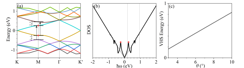
Figure 1: Illustration of the (a) band structure and (b) DOS for twist angle $\theta=4^{\circ}$. The two dotted vertical lines separate the three regimes in positive energies. (c) The twist angle dependence of energy at VHS.

III.2 Injection coefficients at $4^{\circ}$

To clearly show how the interlayer coupling at different twist angles affect the injection, it is constructive to consider the ratio between the obtained results and those results for uncoupled TBG, where the interlayer coupling strength is set as $w_{0}=0$. The uncoupled TBG becomes simply two uncoupled monolayer of graphene, and the injection occurs in each layer only, for which analytic results have been obtained Rioux et al. (2011). The injection in graphene is isotropic with additional relations for the injection coefficients as $\xi_{2}^{xyxy}=-\xi_{2}^{xxyy}$ and $\eta_{12}^{xyxy}=-\eta_{12}^{xxyy}$. Thus in an uncoupled TBG for any twist angle $\theta$ the injection coefficients are just twice of those in graphene, as

$$\xi_{1}^{xx}(\omega)|_{u}= \frac{e^{2}}{\hbar^{2}\omega}\,,\quad\xi_{2}^{xxxx}(\omega)|_{u}=\frac{2\hbar v_{f}^{2}e^{4}}{(\hbar\omega)^{5}}\,,\quad\eta_{12}^{xxxx}(\omega)|_{u}=i\frac{v_{f}^{2}e^{4}}{(\hbar\omega)^{3}}\,.$$ (25)

The normalized injection coefficients are defined as $\overline{\xi}_{1}^{ab}(\omega)=\xi^{ab}_{1}(\omega)/\xi_{1}^{xx}(\omega)|_{u}$, $\overline{\xi}_{2}^{abcd}(\omega)=\xi_{2}^{abcd}(\omega)/\xi_{2}^{xxxx}(\omega)|_{u}$, and $\overline{\eta}_{12}^{gabc}(\omega)=\eta_{12}^{gabc}(\omega)/\eta_{12}^{xxxx}(\omega)|_{u}$, which are dimensionless quantities. In an uncoupled TBG, $\eta_{12}^{xxxx}(\omega)|_{u}$ is a pure imaginary number; with the inclusion of interlayer coupling, $\eta_{12}^{gabc}$ is in general complex, but the calculations show its real part is 2 orders of magnitude smaller than its imaginary part, which will be presented below.

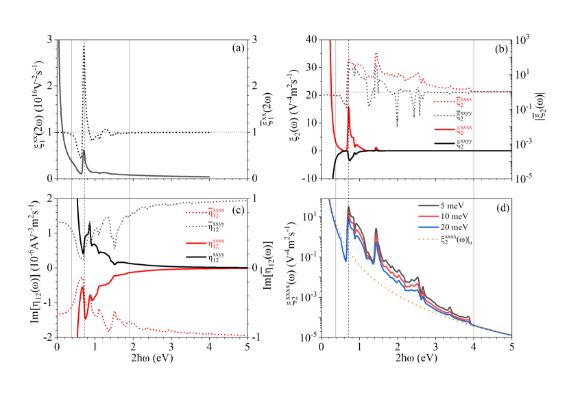
Figure 2: Spectra of injection coefficients of TBG with $\theta=4^{\circ}$ and $\mu=0$. (a) One-photon carrier injection coefficient $\xi_{1}^{xx}(\omega)$, (b) two-photon carrier injection coefficients $\xi_{2}^{xxxx}(\omega)$ and $\xi_{2}^{xxyy}(\omega)$, (c) the imaginary part of coherent current injection coefficients $\eta_{12}^{xxxx}(\omega)$ and $\eta_{12}^{xxyy}(\omega)$. In (a,b,c) the right axis gives the normalized injection coefficients. The vertical solid lines located at $2\hbar\omega=0.38,1.9$ or $4~{}\text{eV}$ divide the whole spectra into three regimes. The vertical dashed lines indicate the energy for the transition at the M point from band $-1$ ($-2$) to $+2$ ($+1$). (d) $\xi^{xxxx}_{2}(\omega)$ at different $\hbar\gamma=5,10,20~{}\text{meV}$.

Figure 2 gives the spectra of these coefficients for a twist angle $4^{\circ}$ at zero chemical potential. Corresponding to three regimes of the band structure, the spectra of injection coefficients can also be divided into three regimes, which are separated by $2\hbar\omega=0.38~{}\text{eV}$ and $1.9~{}\text{eV}$ for $\xi_{1}^{ab}$ and $\eta_{12}^{gabc}$ or $2\hbar\omega=0.38~{}\text{eV}$ and $4~{}\text{eV}$ for $\xi_{2}^{abcd}$. The second boundary is different due to the existence of unique divergence in two-photon absorption. At low energy regime $2\hbar\omega<0.38~{}\text{eV}$, the injection occurs mostly between the bands $\pm$1 in the linear dispersion regime, the results are similar to those of graphene but with a smaller Fermi velocity $v_{f}^{\prime}$. From Eq. (25), the one-photon injection coefficient is the same as the uncoupled TBG because it is independent of the Fermi velocity; however, two-photon carrier injection and two-color coherent current injection show smaller coefficients due to the smaller Fermi velocity. These features are clearly shown by the values $\overline{\xi}_{1}^{xx}=1$, $\overline{\xi}_{2}^{xxxx}$ and $\overline{\eta}_{12}^{xxxx}$ which are approximately constant but less than $1$. In the high energy regime with photon energies $2\hbar\omega>1.9$ eV for $\xi^{xx}_{1}(\omega)$ and $\eta^{xxxx}_{12}(\omega)$, or $2\hbar\omega>4~{}\text{eV}$ for $\xi^{xxxx}_{2}(\omega)$, the coefficients gradually approach the case without interlayer coupling.

In the middle regime, the spectra of injection coefficients contain fruitful fine structures, which are also clearly shown in the normalized injection coefficients. All of them have dips at $2\hbar\omega\approx 0.68~{}\text{eV}$, which are induced by the optical transitions involving the states with smaller DOS shown in Fig. 1 (b). At $2\hbar\omega\approx 0.72~{}\text{eV}$, $\bar{\xi}_{1}^{xx}(\omega)$ appears a peak with a value around 3, which arises from the optical transitions at the VHS. However, both $\bar{\eta}^{xxxx}_{12}(\omega)$ and $\bar{\eta}^{xxyy}_{12}(\omega)$ show local peaks at $2\hbar\omega=0.76~{}\text{eV}$ and $0.85~{}\text{eV}$, respectively. The higher photon energies of these peak locations are because the VHS has zero carriers velocity $v_{ss\bm{k}}^{g}-v^{g}_{s^{\prime}s\prime\bm{k}}$, which lowers and shifts the peak for current injection coefficients. After the peak, the injection coefficients decrease with some fine features (tiny dips), which are induced by the existence of multiple bands. In the whole middle regime, the normalized current injection coefficients are less than 1.

Different from one-photon carrier injection and two-color coherent injection, where the injection coefficients are at the same order of magnitude of graphene, the two-photon carrier injection can be a few hundreds times larger than that of graphene for photon energies $0.72<2\hbar\omega<4~{}\text{eV}$. This is because for these photon energies, both the resonant one-photon optical transition and resonant two-photon optical transition can exist simultaneously, which leads to a double resonance discussed after Eq. (24). To better illustrate its dependence on $\gamma$, we also plot $\xi_{2}^{abcd}(\omega)$ in Fig. 2 (d) for different $\hbar\gamma=5,10,20~{}\text{meV}$. Our calculation indicates that the injection coefficients for the double resonant transitions are approximately proportional to $\gamma^{-1}$.

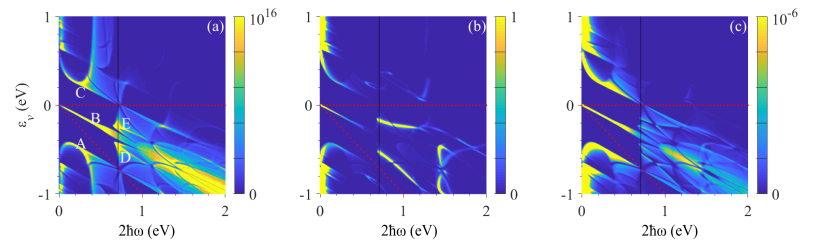
Figure 3: Electron energy resolved injection coefficients (a) $\left(\frac{2\hbar\omega}{1\text{eV}}\right)^{2}\widetilde{\xi}_{1}^{xx}(\epsilon_{v},2\omega)$, (b) $\left(\frac{\hbar\omega}{1\text{eV}}\right)^{4}\widetilde{\xi}_{2}^{xxxx}(\epsilon_{v},\omega)$, and (c) $\left(\frac{2\hbar\omega}{1\text{eV}}\right)^{3}\text{Im}[\widetilde{\eta}_{12}^{xxxx}(\epsilon_{v},\omega)]$. The two dotted lines give $\epsilon_{v}=\mu$ and $\epsilon_{v}=\mu-\hbar\omega$ for $\mu=0~{}\text{eV}$.

III.3 Electron energy resolved injection coefficients at $\theta=4^{\circ}$

The injection processes can be better understood by using the electron energy resolved injection coefficients, from which the contributions from different electron energies can be visualized. As an example, for the one-photon injection, it is defined as

$$\widetilde{\xi}_{1}^{(\nu);ab}(\epsilon_{v},2\omega)= 4\pi\left(\frac{e}{\hbar\omega}\right)^{2}\sum_{ss^{\prime}}\int\frac{d\bm{k}}{\left(2\pi\right)^{2}}\left(v_{ss^{\prime}\bm{k}}^{(\nu);a}\right)^{\ast}v_{ss^{\prime}k}^{(\nu);b}\delta(\varepsilon_{s^{\prime}\bm{k}}-\epsilon_{v})\hbar\delta(\varepsilon_{s\bm{k}}-\epsilon_{v}-2\hbar\omega)\,,$$ (26)

from which the injection coefficients can be obtained as

$$\xi_{1}^{(\nu);ab}(2\omega)=\int d\epsilon_{v}\left[\Theta(\mu-\epsilon_{v})-\Theta(\mu-2\hbar\omega-\epsilon_{v})\right]\widetilde{\xi}_{1}^{(\nu);ab}(\epsilon_{v},2\omega)\,.$$ (27)

Similar definitions can be applied to get $\widetilde{\xi}_{2}^{dabc}(\epsilon_{v},\omega)$ and $\widetilde{\eta}_{12}^{gabc}(\epsilon_{v},\omega)$. Equation (27) shows that only the electrons states with energies $\mu-2\hbar\omega<\epsilon_{v}<\mu$ contribute to the injection process. For uncoupled TBG or for graphene, the injection occurs as $\epsilon_{v}=-\hbar\omega<-|\mu|$.

Figure 3 shows electron energy resolved injection coefficients $\widetilde{\xi}_{1}^{xx}(\epsilon_{v},2\omega)$, $\widetilde{\xi}_{2}^{xxxx}(\epsilon_{v},\omega)$, and $\widetilde{\eta}_{12}^{xxxx}(\epsilon_{v},\omega)$. Taking $\widetilde{\xi}_{1}^{xx}(\epsilon_{v},2\omega)$ as an example, the main contributions locate in the regions identified by the optical transitions between bands A: $-2\to-1$, B: $-1\to 1$, C: $1\to 2$, D: $-2\to 1$, E: $-1\to 2$, and F: for transitions from or to higher energy bands. The regions D and E include the optical transitions around the VHS. At $\mu=0$, the electron energy resolved injection coefficients mostly locate in the region $-2\hbar\omega<\epsilon_{v}<0$ given by the dashed red lines, including the regions B, E, and D. For nonzero $\mu$, contributions from other regions can be tuned on or off, which will be discussed in next section.

III.4 Chemical potential dependence

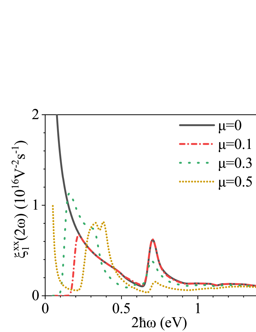
Figure 4: Spectra of injection coefficients (a) $\xi_{1}^{xx}(2\omega)$, (b) $\xi_{2}^{xxxx}(\omega)$, (c) $\text{Im}[\bar{\eta}_{12}^{xxxx}(\omega)]$ for chemical potentials $\mu$=$0,0.1,0.3,0.5~{}\text{eV}$.

Now we consider how doping affects the injection coefficients. Figure 4 shows the spectra for $\mu=0,0.1,0.3,0.5~{}\text{eV}$ at $4^{\circ}$. For $\mu=0.1~{}\text{eV}$, the chemical potential is in the linear dispersion regime. Following the results of graphene, the chemical potential induced effective band gap is $E_{g}=2|\mu|$, thus all injection coefficients show an onset energy at $2\hbar\omega=0.2~{}\text{eV}$. The new transitions from the $+1$ band to higher bands (from region C in Fig. 3) require higher photon energies and the contribution is negligible, so the results after the effective gap are almost the same as those results at zero chemical potential. When the chemical potential increases to $0.3~{}\text{eV}$, which still lies in the +1 band, a direct consideration of the effective gap should be as high as $0.6~{}\text{eV}$. However, the higher doping level makes transitions from the +1 band to higher bands (from the region C in Fig. 3) requires less photon energy, which reduces the effective gap to $0.15~{}\text{eV}$. When the chemical potential is $0.5~{}\text{eV}$, the onset energy goes to even smaller around 0. From Fig. 3, all injections contributed from the regions B, D, and E are suppressed, but region C contributes greatly for small photon energies, and enhances the one-photon carrier injection for photon energies between $0.27~{}\text{eV}$ and $0.31~{}\text{eV}$, and two-photon carrier injection and coherent current injection for photon energies between $0.27~{}\text{eV}$ and $0.5~{}\text{eV}$.

III.5 Twisted angle dependence

Figure 5: Photon energy dependence of the normalized injection coefficients (a) $\overline{\xi}_{1}^{xx}(\omega)$, (b) $\overline{\xi}_{2}^{xxxx}(\omega)$, and (c) $\text{Im}[\eta_{12}^{xxxx}(\omega)]$ for different twist angles $3^{\circ}$, $5^{\circ}$, $7^{\circ}$, $9^{\circ}$, and $10^{\circ}$.

Figure 5 gives the normalized injection coefficients for $\theta=3^{\circ}$, $5^{\circ}$, $7^{\circ}$, $9^{\circ}$ and $10^{\circ}$. For $\theta>10^{\circ}$, the continuum model for electronic states is not suitable Bistritzer and MacDonald (2011). The spectra at different twist angles show very similar features to that of $4^{\circ}$. With increasing $\theta$, the peaks/valleys are shifted to larger photon energies, which is consistent with our analysis of the band structure. These results indicate that optical injection processes can be effectively tuned by the twisted angle.

IV CONCLUSION

We have theoretically investigated one- and two-photon carrier injection and two-color coherent current injection in twisted bilayer graphene for twist angles between $3^{\circ}$ and $10^{\circ}$, where the injection coefficients are numerically evaluated at zero temperature for different chemical potentials. Compared to the results for graphene, the spectra of injection coefficients in twisted bilayer graphene exhibit different features in three energy regimes: in the low energy regime where the band structure is approximately linear, all injection coefficients have similar behaviors as that of graphene, but with a different amplitude determined by the renormalized Fermi velocity; for very high photon energies, all injection coefficients are almost the same as that of graphene, because the involved electronic states have large energies which are not effectively affected by the interlayer coupling; and in the middle regime, the carrier injection coefficients show resonant peaks around the Van Hove Singularity, while the current injection coefficients are smaller because the injected carriers around the Van Hove singularity have zero velocity. All these results are characterized from an electron energy resolved injection coefficients. Due to the existence of multiple bands, the degenerate two-photon optical transition processes can have double resonant optical transitions between the initial, the intermediate, and the final states, which lead to a divergent two-photon carrier injection and a finite two-color current injection.

With the decrease of the twist angle, these features shift to low photon energies, suggesting twist angle tunable applications in far infrared or Terahertz wavelength. The optical injection for very small twist angles are not investigated in this work, mostly due to the difficulties in the numerical calculation that require a large number of plane wave expansion to get accurate band eigenstates. However, at these angles, the strong carrier-carrier interaction may lead to a different behavior of the optical injectionBhat and Sipe (2005), which is worth for a future exploration.

This work mostly focuses on the comparison of the injection coefficients of twisted bilayer graphene and those of graphene, and there also exists other important injection processes appearing only in twisted bilayer graphene that are worth to be explored but not discussed here. For example, the stacking of two layers of graphene opens the responses along the perpendicular directionGao et al. (2020), which are usually ignored in a monolayer graphene, the two-color optical injection tensors have nonzero components for oblique incident light. Moreover, due to the lower symmetry, a single color light with an appropriate polarization is also possible to inject currents.