Hadronic Parity Violation from 4-quark Interactions

Abstract

We present an exploratory investigation of the parity odd $\Delta I=1$ pion-nucleon coupling $h_{\pi}^{1}$ from lattice QCD. Based on the PCAC relation, we study the parity-conserving effective Hamiltonian and extract the coupling by determining the nucleon mass splitting arising from the effective 4-quark interactions using the Feynman-Hellmann theorem. We present preliminary results of the mass shift for a $32^{3}\times 64$ ensemble of $N_{f}=2+1+1$ twisted mass fermions at pion mass $260\,\mathrm{MeV}$ and lattice spacing $a=0.097\,\mathrm{fm}$.

1 Introduction

The study of parity (P) violation in the weak sector of the Standard Model started in the 1960s, immediately following the seminal paper by Lee and Yang [1] and the first experimental evidence by Madam Wu and collaborators [2]. Despite countless experiments over the last six decades, the study of hadronic parity violation (HPV) is still of importance. Our focus here is on flavor-conserving hadronic interactions. For the latter there is an overwhelming background from strong interaction, governed by quantum chromodynamics (QCD), and electromagnetic interaction. In particular, since the strong coupling is significantly stronger than the weak coupling, extracting the smaller signal contribution from P-violating hadronic weak interaction is rendered a difficult task.

The most used theory model of HPV is based on the exchange of single light mesons, as developed by Desplanques, Donoghue and Holstein (DDH) [3]. This model contains seven independent coupling constants. A long-standing problem in HPV is the determination of these P-violating coupling constants. Of particular interest to us is the $\Delta I=1$ pion-nucleon coupling $h_{\pi}^{1}$. This particular transition is suppressed for the weak charged current, and therefore serves as a probe for the in this case dominant neutral current. Since the underlying weak operators and the Wilson coefficients are known, the only remaining work is the calculation of the hadronic matrix elements, either through non-perturbative methods or through fits to experimental data.

On the side of experiments, a recent measurement by the NPDGamma collaboration produced the first experimental determination of $h_{\pi}^{1}$ [4]. On the theoretical side, however, there has been only one study using lattice QCD [5]. Despite the fact that this theoretical determination overlaps very nicely with the experimental measurement, one needs to be careful when considering this result. The study was done on a single lattice with pion mass of 390 MeV, and contributions from the so-called "quark-loop" diagrams were not considered. The author also used 3-quark interpolators for the $N\pi$ final state in order to simplify Wick contractions. These issues were pointed out by Feng, Guo and Seng (FGS) in their 2018 paper [6], where they also proposed a different strategy for determining $h_{\pi}^{1}$. They proposed to get rid of the $N\pi$ final state by using partially conserved axial current (PCAC) relations and to determine the coupling constant in terms of the induced relative mass shift between proton and neutron. Our work serves as a benchmark for this newly proposed technique.

2 The 4-quark operators

According to the DDH model, the parity violating weak Lagrangian, in the hadronic sector, is written as

$$\mathcal{L}_{PV}^{w}=\frac{h_{\pi}^{1}}{\sqrt{2}}\,\bar{N}\,\left(\vec{\tau}\times\vec{\pi}\right)_{3}\,N+\cdots\,.$$ (1)

Here $N=(p\;n)^{T}$ is the isospin doublet of nucleons and $\vec{\tau}$ are the Pauli matrices. One then obtains the coupling constant $h_{\pi}^{1}$ from the hadronic matrix element

$$h_{\pi}^{1}=-\frac{i}{2m_{N}}\lim_{p_{\pi}\to 0}\langle n\pi^{+}|\mathcal{L}_{PV}^{w}(0)|p\rangle\,,$$ (2)

where $m_{N}$ is the average nucleon mass. At low energies $\mathcal{L}_{PV}^{w}$ can be expressed in terms of seven independent P-odd 4-quark operators [7]

$$\mathcal{L}_{PV}^{w}=-\frac{G_{F}}{\sqrt{2}}\,\frac{\sin^{2}\theta_{w}}{3}\sum_{i}\left(C_{i}^{(1)}\theta_{i}+S_{i}^{(1)}\theta_{i}^{(s)}\right)\,,$$ (3)

where

$$\theta_{1} =\bar{q_{a}}\gamma_{\mu}q_{a}\bar{q}_{b}\gamma_{\mu}\gamma_{5}\tau_{3}q_{b},\;\;\;\;\;\;\theta_{2}=\bar{q}_{a}\gamma_{\mu}q_{b}\bar{q}_{b}\gamma_{\mu}\gamma_{5}\tau_{3}q_{a},$$ (4)

$$\theta_{3} =\bar{q}_{a}\gamma_{\mu}\gamma_{5}q_{a}\bar{q}_{b}\gamma_{\mu}\tau_{3}q_{b},\;\;\;\;\;$$

$$\theta_{1}^{(s)} =\bar{s}_{a}\gamma_{\mu}s_{a}\bar{q}_{b}\gamma_{\mu}\gamma_{5}\tau_{3}q_{b},\;\;\;\;\;\theta_{2}^{(s)}=\bar{s}_{a}\gamma_{\mu}s_{b}\bar{q}_{b}\gamma_{\mu}\gamma_{5}\tau_{3}q_{a}\,,$$

$$\theta_{3}^{(s)} =\bar{s}_{a}\gamma_{\mu}\gamma_{5}s_{a}\bar{q}_{b}\gamma_{\mu}\tau_{3}q_{b},\;\;\;\;\;\theta_{4}^{(s)}=\bar{s}_{a}\gamma_{\mu}\gamma_{5}s_{b}\bar{q}_{b}\gamma_{\mu}\tau_{3}q_{a}\,.$$

Here, $q=(u\;d)^{T}$ is the light quark doublet, $G_{F}$ is the Fermi constant and $\theta_{w}$ is the weak mixing angle. $C_{i}$ and $S_{i}$ are well known Wilson coefficients. The values of these coefficients, at the scale $\Lambda_{\chi}\approx 1\,\mathrm{GeV}$, are [13]

$$C^{(1)}(\Lambda_{\chi}) =\begin{pmatrix}-0.055,&0.810,&-0.627\end{pmatrix}$$ (5)

$$S^{(1)}(\Lambda_{\chi}) =\begin{pmatrix}5.09,&-2.55,&4.51,&-3.36\end{pmatrix}$$

The presence of a soft pion in the final state of the matrix element greatly complicates the calculation for reasons pointed out in [8]. FGS proposed to get rid of the soft pion by relating this matrix element to a parity conserving counterpart, using the PCAC relation

$$\lim_{p_{\pi}\to 0}\langle a\pi^{i}|\hat{O}|b\rangle=\frac{i}{F_{\pi}}\langle a|\left[\hat{O},\hat{Q}_{A}^{i}\right]|b\rangle\,,$$ (6)

where $F_{\pi}=92.1\,\mathrm{MeV}$ is the pion decay constant and $\hat{Q}_{A}^{i}$ are the axial charges. This means instead of calculating $\langle n\pi^{+}|\mathcal{L}_{PV}^{w}|p\rangle$, we can simply compute $\langle n|\left[\mathcal{L}_{PV}^{w},\hat{Q}_{A}^{i}\right]|p\rangle$. At the operator level, the PCAC relation yields

$$\left[\theta_{q},\hat{Q}^{i}_{A}\right]=i\epsilon^{3ij}\theta^{\prime}_{q(j)},\;\;\;\;\;\left[\theta_{q}^{(s)},\hat{Q}^{i}_{A}\right]=i\epsilon^{3ij}\theta_{q(j)}^{(s)^{\prime}}\,,$$ (7)

where $\theta^{\prime}_{q}$ and $\theta^{(s)^{\prime}}_{q}$ are the parity even 4 quark operators defined as

$$\theta^{{}^{\prime}\phantom{(s)}}_{1} =\bar{q}_{a}\gamma_{\mu}q_{a}\bar{q}_{b}\gamma_{\mu}\tau_{3}q_{b}\,,\quad \theta^{{}^{\prime}\phantom{s}}_{2} =\bar{q}_{a}\gamma_{\mu}q_{b}\bar{q}_{b}\gamma_{\mu}\tau_{3}q_{a}\,,$$

$$\theta^{{}^{\prime}\phantom{(s)}}_{3} =\bar{q}_{a}\gamma_{\mu}\gamma_{5}q_{a}\bar{q}_{b}\gamma_{\mu}\gamma_{5}\tau_{3}q_{b}\,,$$ (8)

$$\theta_{1}^{(s)^{\prime}} =\bar{s}_{a}\gamma_{\mu}s_{a}\bar{q}_{b}\gamma_{\mu}\tau_{3}q_{b}\,,\quad \theta_{2}^{(s)^{\prime}} =\bar{s}_{a}\gamma_{\mu}s_{b}\bar{q}_{b}\gamma_{\mu}\tau_{3}q_{a}\,,$$

$$\theta_{3}^{(s)^{\prime}} =\bar{s}_{a}\gamma_{\mu}\gamma_{5}s_{a}\bar{q}_{b}\gamma_{\mu}\gamma_{5}\tau_{3}q_{b}\,,\quad \theta_{4}^{(s)^{\prime}} =\bar{s}_{a}\gamma_{\mu}\gamma_{5}s_{b}\bar{q}_{b}\gamma_{\mu}\gamma_{5}\tau_{3}q_{a}\,.$$ (9)

This maps the matrix elements of P-odd hadronic operators to matrix elements to P-even ones to leading order in chiral perturbation theory

$$\lim_{p_{\pi}\to 0}\langle n\pi^{+}|\mathcal{L}_{PV}^{w}(0)|p\rangle\approx-\frac{\sqrt{2}i}{F_{\pi}}\langle p|\mathcal{L}_{PC}^{w}(0)|p\rangle=\frac{\sqrt{2}i}{F_{\pi}}\langle n|\mathcal{L}_{PC}^{w}(0)|n\rangle\,,$$ (10)

where $\mathcal{L}_{PC}^{w}$ is the following auxiliary parity conserving Lagrangian

$$\mathcal{L}_{PC}^{w}=-\frac{G_{F}}{\sqrt{2}}\frac{\sin^{2}\theta_{W}}{3}\sum_{i}\left(C_{i}^{(1)}\theta^{\prime}_{i}+S^{(1)}_{i}\theta^{(s)^{\prime}}_{i}\right)\,.$$ (11)

Since the PCAC relation holds at the operator level, the Wilson coefficients are identical to those in $\mathcal{L}_{PV}^{w}$. The matrix element can be determined in terms of the neutron-proton mass splitting $(\delta m_{N})_{4q}\equiv(m_{n}-m_{p})_{4q}$ induced by the Lagrangian $\mathcal{L}_{PC}^{w}$

$$(\delta m_{N})_{4q}=\frac{1}{m_{N}}\langle p|\mathcal{L}_{PC}^{w}(0)|p\rangle=-\frac{1}{m_{N}}\langle n|\mathcal{L}_{PC}^{w}(0)|n\rangle\,.$$ (12)

Combining everything, one obtains the coupling constant $h_{\pi}^{1}$ as

$$h_{\pi}^{1}\approx-\frac{(\delta m_{N})_{4q}}{\sqrt{2}F_{\pi}}\,.$$ (13)

3 Mass shift from Feynman-Hellmann theorem

According to Feynman-Hellmann theorem (FHT) [9, 10], a perturbation in the Hamiltonian of the form $H\to H+\lambda H_{\lambda}$ corresponds to a variation in the spectrum as

$$\frac{\partial E_{n}}{\partial\lambda}=\langle n|H_{\lambda}|n\rangle\,.$$ (14)

This straightforward relation of first order in perturbation theory can be used to extract matrix elements in lattice QCD [11]. Considering the 2-point nucleon-nucleon correlator in the presence of an external source $\lambda$

$$C_{\lambda}(t) =\langle\lambda|N(t)\bar{N}(0)|\lambda\rangle=\frac{1}{Z_{\lambda}}\int\mathcal{D}\psi\,\mathcal{D}\bar{\psi}\;N(t)\bar{N}(0)\;e^{-S-S_{\lambda}}\,,$$ (15)

where the source $\lambda$ is coupled to the 4-quark current introduced in the previous section

$$S_{\lambda}=\lambda\int d^{4}x\;\mathcal{L}_{PC}^{w}(x)\,.$$ (16)

The derivative of the perturbed correlator gives

$$-\frac{\partial C_{\lambda}}{\partial\lambda}\bigg{|}_{\lambda=0} =\frac{\partial Z_{\lambda}}{\partial\lambda}\bigg{|}_{\lambda=0}\frac{C(t)}{Z}+\frac{1}{Z}\int\mathcal{D}\psi\mathcal{D}\bar{\psi}e^{-S}\int d^{4}x\;\mathcal{L}_{PC}^{w}(x)N(t)\bar{N}(0)$$ (17)

$$=-C(t)\int d^{4}x\;\langle\Omega|\mathcal{L}_{PC}^{w}(x)|\Omega\rangle+\int d^{4}x\;\langle\Omega|\mathcal{T}\{N(t)\mathcal{L}_{PC}^{w}(x)\bar{N}(0)\}|\Omega\rangle\,.$$

The first term vanishes due to lattice symmetries. The second term is effectively $\sum_{x}\langle p|\mathcal{L}_{PC}^{w}(x)|p\rangle$. The energy shift is then obtained from the linear response of the effective mass

$$\frac{\partial m_{N}}{\partial\lambda}\bigg{|}_{\lambda=0}(t,\tau)=\frac{1}{\tau}\left[\frac{\partial_{\lambda}C_{\lambda}(t)}{C(t)}-\frac{\partial_{\lambda}C_{\lambda}(t+\tau)}{C(t+\tau)}\right]\,.$$ (18)

Here $C$ is the unperturbed correlator ($\lambda=0$). We compute the right-hand side of Eq. (18), which is proportional to the mass shift $(\delta m_{N})_{4q}$.

4 Lattice Setup

The determination of $\langle p|\mathcal{L}_{PC}^{w}|p\rangle$ requires calculation of three kinds of diagrams. Figure 1 gives a visual representation of the 3 diagrams. There are also quark-disconnected diagrams, which vanish in the limit of exact $SU(2)$ flavor symmetry and are neglected in the present approach.

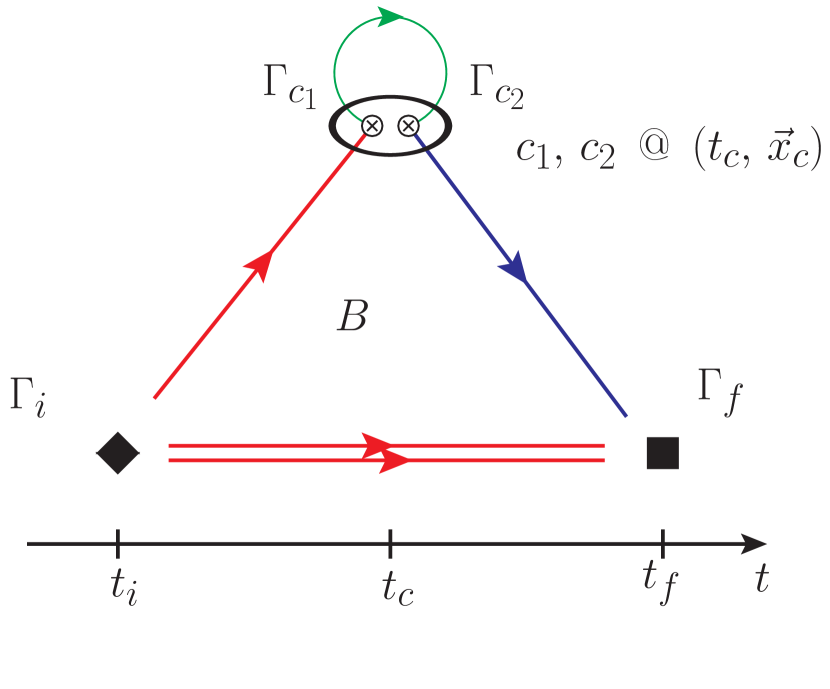
(a) B-type

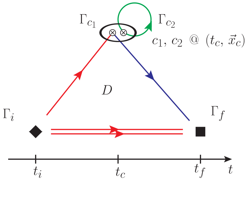
(b) D-type

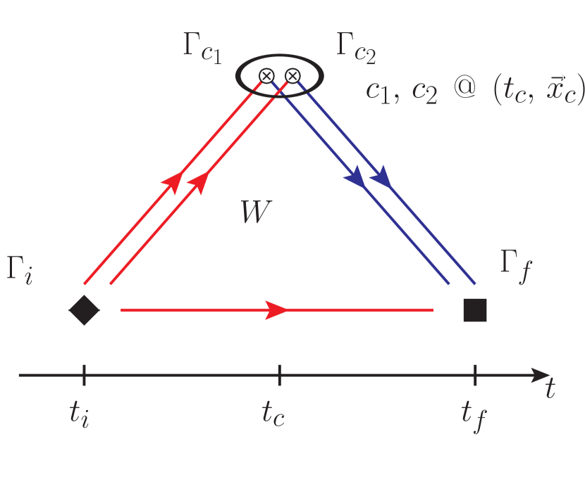
(c) W-type

Figure 1: The 3 kinds of diagrams under consideration. (Note that $c_{1}$ and $c_{2}$ shown separately for clarity. Physically they are the same point on the lattice.) The color coding for quark propagator types is as follows: red = point-to-all, green = stochastic and blue = sequential propagator.

We use sequential propagator techniques to calculate these diagrams. For B and D-type, we consider one fully time-, spin-, and color-diluted stochastic source $\xi^{(k)}$, where $k$ denotes the composite dilution index,

$$\xi^{(t,\beta,b)}(x)_{\alpha\atop a} =\delta_{\alpha\beta}\,\delta_{ab}\,\delta_{x_{0}t}\,\xi(\vec{x})\,,$$ (19)

$$\xi(\vec{x}) \sim\frac{1}{\sqrt{2}}\,\left(Z_{2}+iZ_{2}\right)\quad\mathrm{~{}iid}\,.$$ (20)

With the corresponding propagator $\phi_{f}^{(k)}=D_{f}^{-1}\,\xi^{(k)}$ for quark flavor $f$ we use the stochastic representation of the $x_{c}\to x_{c}$ quark propagator

$$L_{f}(x_{c})_{\alpha\beta\atop ab}=\sum\limits_{k}\,\phi_{f}^{(k)}(x_{c})_{\alpha\atop a}\xi^{(k)*}(x_{c})_{\beta\atop b}$$ (21)

such that $E\left[L_{f}(x_{c})\right]=S_{f}(x_{c};x_{c})_{\alpha\beta\atop ab}$, i.e. the stochastic expectation behaves like a quark loop.

Sequential sources for B and D-type diagrams are then built accordingly as

$$\Phi_{B}(x_{c};x_{i}) :=\Gamma_{c_{2}}\,\bar{L}(x_{c})\,\Gamma_{c_{1}}\,S(x_{c};x_{i})$$ (22)

$$\Phi_{D}(x_{c};x_{i}) :=\text{Tr}\left[\Gamma_{c_{2}}\,\bar{L}(x_{c})\right]\,\Gamma_{c_{1}}\,S(x_{c};x_{i})\,.$$ (23)

For W-type diagrams we consider a set of scalar noise sources with the properties

$$E\left[\eta^{(k)}(x)\right]=0,\hskip 20.00003ptE\left[\eta^{(k)}(x)\,\eta^{(l)}(y)\right]=\delta_{kl}\,\delta_{x,y}\,,$$ (24)

with $E$ the expectation value, and insert such a noise between a pair of propagators to obtain a W-type propagator

$$\tilde{W}^{(k)}(\Gamma_{c})=\sum_{x_{c}}S(x_{f};x_{c})\,\Gamma_{c}\,\eta^{(k)}(x_{c})\,S(x_{c};x_{i})\,.$$ (25)

The expectation of a product of two such propagators is needed for the W diagram.

For the simulation, we have used $N_{f}=2+1+1$ clover-improved twisted mass lattice ensemble $cA211.30.32$ produced by the ETMC collaboration [12]. Table 1 lists the parameters of the gauge ensemble.

$L^{3}\times T$	$a[fm]$	$a\mu_{l}$	$am_{\pi}$	$m_{\pi}L$	$m_{\pi}[MeV]$
$32^{3}\times 64$	$0.097$	$0.00300$	$0.12530\,(16)$	$4.01$	$261.1\,(1.1)$

Table 1: Relevant parameters of gauge ensemble $cA211.30.32$. For more details we refer to Ref. [12].

The propagators are source and sink smeared with Wuppertal smearing. APE smearing is also performed to smooth the gauge.

For the loops in B and D-type diagrams we were limited to only one stochastic source due to computational cost. We tried overcoming this by calculating at 8 different source coordinates per configuration. For W-type diagrams we used 8 stochastic sources and 2 source coordinates per configuration.

5 Results

In this work we present results for the 3 operators in the light quark sector, Eq. (8). Figure 2 shows the 3-point correlators for the 3 operator insertions (note we have dropped the ^′ in the operator names). The symmetry between $\theta_{1}$ and $\theta_{3}$ is expected at least at tree level. $\theta_{2}$ has considerably more noise. We suspect that it could be due to mixing under renormalization with the lower dimensional operator $\bar{\psi}\,\gamma_{5}\,\psi$.

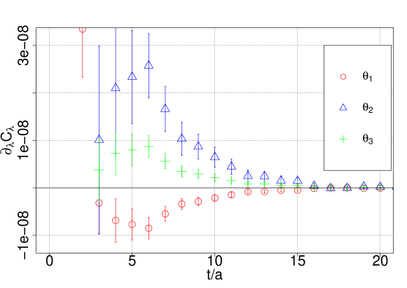
Figure 2: 3-point correlators with the 4-quark operator insertions

The mass shift is calculated according to FHT. Figure 3 shows the $t$ and $\tau$ dependence of the shift for $\theta_{1}$. The noise becomes prohibitively large for $t/a\geq 12$. Figure 4 shows the mass shift fitted in range $\tau/a\in[3,7]$ for the timeslices $t/a\in[6,11]$.

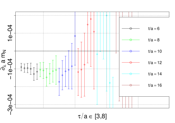
Figure 3: Large $t$ and $\tau$ dependence of $\theta_{1}$ (for each timeslice the data is shown for the range $\tau/a\in[3,8]$ )

Given the exploratory nature of this study, we do not intend to determine a value for the coupling $h_{\pi}^{1}$ here yet. However, the discrepancy between the value obtained by naively adding these three plateau values with corresponding Wilson coefficients and the experimental value most likely stem from the missing renormalization process and the missing strange contributions. We are currently working on both.

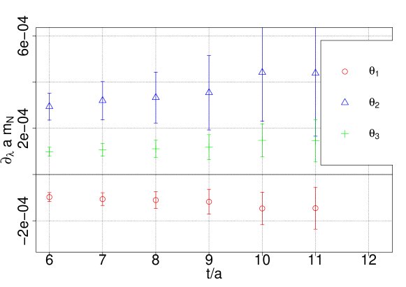
Figure 4: Mass shifts fitted over a range of $\tau/a\in[3,7]$ for each timeslice

6 Conclusion

This work represents an exploratory benchmark for a newly proposed technique to measure the coupling $h_{\pi}^{1}$. So far the results are promising. Non-zero signal has been observed for all diagrams with all Dirac structures. The mass shifts for individual operators have also turned out to be non-zero. Thus the practical simplification of signal extraction envisioned by FGS is reachable.

Work on the strange operators and renormalization of the 4-quark lattice operators is currently ongoing. A parallel computation with traditional 3-point technique is also underway in order to compare cost and signal quality with the current work. Once our setup is optimized, we aim at a calculation directly at physical pion mass to obtain a theoretical estimate for $h_{\pi}^{1}$, which is rigorously comparable to the experimental determination.

References

- [1] T. D. Lee and C. N. Yang, Phys. Rev. 104, 204 (1956)
- [2] C. S. Wu et al., Phys. Rev. 105, 1413 (1957)
- [3] B. Desplanques, J. F. Donoghue and B. R. Holstein, Ann. Phys. (N. Y.), 124, 449 (1980)
- [4] [NDPGamma] D. Blyth et al., Phys. Rev. Lett. 121, 242002 (2018), 1807.10192
- [5] J. Wasem, Phys. Rev. C85, 022501 (2012), 1108.1151
- [6] X. Feng, F. K. Guo and C. Y. Seng, Phys. Rev. Lett. 120, 181801 (2018), 1711.09342
- [7] D. B. Kaplan and M. J. Savage, Nucl. Phys. A556, 653 (1993)
- [8] F. K. Guo and C. Y. Seng, Eur. Phys. J. C 79, 22 (2019), 1809.00639
- [9] R. P. Feynman, Phys. Rev. 56, 340 (1939)
- [10] H Hellmann, Einführung in die Quantenchemie (Franz Deuticke, 1937) p. 285
- [11] C. Bouchard, Phys. Rev. D 96, 014504 (2017), 1612.06963
- [12] G. Bergner et al., PoS LATTICE2019, 181 (2020), 2001.09116
- [13] B. C. Tiburzi, Phys. Rev. D 85 (2012), 054020 doi:10.1103/PhysRevD.85.054020