Spillovers of US Interest Rates
Monetary Policy & Information Effects

Abstract

This paper quantifies the international spillovers of US monetary policy by exploiting the high-frequency movement of multiple financial assets around FOMC announcements. I use the identification strategy introduced by Jarocinski [2020] to identify two FOMC shocks: a pure US monetary policy and an information disclosure shock. These two FOMC shocks have intuitive and very different international spillovers. On the one hand, a US tightening caused by a pure US monetary policy shock leads to an economic recession, an exchange rate depreciation and tighter financial conditions. On the other hand, a tightening of US monetary policy caused by the FOMC disclosing positive information about the state of the US economy leads to an economic expansion, an exchange rate appreciation and looser financial conditions. Ignoring the disclosure of information by the FOMC biases the impact of a US monetary policy tightening and may explain recent atypical findings.

Keywords: Monetary policy, Emerging markets, Exchange Rates, Monetary Policy Spillovers.

JEL Codes: F40, F41, E44, E51.

1 Introduction

The international spillovers of US monetary policy is a classic question in international macroeconomics, going back to Fleming [1962], Mundell [1963], Dornbusch [1976] and Frenkel [1983]. The status of the US dollar as the global reserve currency, unit of account, invoice of international trade and its dominant role in financial markets implies that the Federal Open Market Committee’s (FOMC) policy decisions have spillover effects on the rest of the world. In recent years, the conventional view that a US monetary tightening leads to negative international spillovers such as a recession, exchange rate depreciation and financial distress (Svensson and Van Wijnbergen [1989], Obstfeld and Rogoff [1995], Betts and Devereux [2000]), has been challenged. In fact, a recent literature has found opposite empirical results, an increase in the US monetary policy rate has been associated with a depreciation of the US dollar and an economic boom and looser financial conditions in the rest of the world (Stavrakeva and Tang [2019], Ilzetzki and Jin [2021]). In this paper, I show that the atypical dynamics documented in this recent literature are can be explained by the disclosure of information about the US economy that takes place around FOMC meetings. This “information disclosure” effect contaminates the identification of monetary policy shocks and biases the estimates of the international spillovers of US monetary policy shocks. Controlling for this information disclosure effect re-establishes the conventional view that a US monetary tightening leads to a recession, exchange rate depreciation and tighter financial conditions.

The recent literature estimating atypical effects of US monetary policy shocks has identified them using the standard high frequency identification strategy, i.e. as unexpected movements in interest rates around FOMC announcements, as in Gertler and Karadi [2015] and Nakamura and Steinsson [2018]. However, FOMC announcements both convey decisions about policy rates and disclose information about the present and future state of the US economy. Both Advanced (AE) and Emerging Market (EM) economies depend heavily on the US business cycle (for instance, because of its international trade with the US or because of the impact of the US economy on commodity goods’ prices) or on the conditions in US financial markets (for example, due to the appetite for AEs and EMs’ sovereign and corporate bonds and/or equity markets). As a result, these economies are affected by both the FOMC’s policy decisions and the new information disclosed by the FOMC. Therefore, separately identifying US monetary policy shocks from information disclosure shocks is essential to study the impact of US monetary policy on EM economies.

In line with this argument, I estimate a panel SVAR model using an identification scheme that allows me to separate two FOMC shocks: a pure US monetary policy shock (MP shock) and an information-disclosure shock (ID shock). I tell them apart using the methodology introduced by Jarociński and Karadi [2020] which imposes sign restrictions on the co-movement of the high-frequency surprises of interest rates and the S&P 500 around FOMC meetings. This co-movement is informative as standard theory unambiguously predicts that a monetary policy tightening shock should lead to lower stock market valuation. This is because a monetary policy tightening decreases the present value of future dividends by increasing the discount rate and by deteriorating present and future firm’s profits and dividends. Thus, MP shocks are identified as those innovations that produce a negative co-movement between these high-frequency financial variables. On the contrary, innovations generating a positive co-movement between the interest rates and the S&P 500 correspond to ID shocks. This is a shock that occurs systematically at the time of the central bank policy announcements, but that is different from the standard monetary policy shock. By separately identifying these two structural shocks into a panel SVAR, I find that MP shocks produce conventional international spillovers, i.e. a recession, exchange rate depreciation and financial distress. On the contrary, an ID shock produces an economic expansion, an exchange rate appreciation and looser financial conditions.

Then, I argue that the recently found atypical dynamics can be attributed by not controlling for the systematic disclosure of information around FOMC meetings. I show that following the standard high frequency identification scheme to identify US interest rate shocks leads to dynamics which are an average of those arising from a MP and ID shock. In particular, this leads to a US interest rate tightening associated with a significant expansion of industrial production and equity indexes for both AE and EM economies. Overall, I argue that not controlling for the information disclosure around FOMC meetings biases the quantifying of international spillovers of US interest rates.

Related literature. This paper relates to three main strands of literature. First, this paper contributes to a long strand of literature which has focused on identifying and quantifying the international spillovers of US monetary policy shocks and their transmission channels. A significant share of this literature has found that a US tightening is associated with negative international spillovers such as an economic recession, an exchange rate depreciation or fall of the value of the country’s currency and tighter overall financial conditions. Examples of this literature are Eichenbaum and Evans [1995] and Uribe and Yue [2006] using data from the 1980s, 1990s, and more recently Dedola et al. [2017], Vicondoa [2019] using data up to the late 2000s. During the rest of the paper I will refer to these results as the conventional view or impact of a US tightening. The contribution to this literature is twofold. First, this paper innovates by introducing an identification scheme that clearly purges any information content included in US monetary policy decisions and finds that conventional results still hold for a time sample of the 2000s and 2010s. Second, this paper contributes to the literature by empirically studying the international spillovers of the disclosure of information by the FOMC as a transmission channel of US interest rates. I show that this transmission channel is quantitatively sizable and has not been considered by the previous literature as a meaningful transmission channel of US interest rates.

This paper also relates to a more recent literature in international economics which have found an atypical association between the US interest rates and AE and EM dynamics. Particularly, Ilzetzki and Jin [2021] argue that there has been a significant change over time in the transmission of US monetary policy shocks on the rest of the world. The authors find that while in the 1980s and early 1990s a US tightening lead to the conventional results described in the previous paragraph, in the last two decades there has been a shift whereby increases in US interest rates depreciate the US dollar but stimulate the rest of the world economy. The authors label this shift as a puzzling change in the transmission of US interest rates. Consequently, in the rest of the paper I will refer to these responses of AEs and EMs to a US tightening as atypical dynamics. Another example of these atypical dynamics is Canova [2005] which finds that after a US tightening, Latin American currencies appreciate while the conventional view would expect a currency depreciation. I contribute to this literature by introducing an identification scheme that deconstruct shocks around FOMC announcements following the methodology introduced by Jarociński and Karadi [2020]. This identification scheme allows me to identify an information disclosure shock which entirely explains the atypical dynamics found by this recent literature. Additionally, this identification scheme allows me to identify a pure US monetary policy shock, which re-establishes the results presented by the conventional view. Consequently, by deconstructing monetary policy shocks I am able to match both the conventional and atypical results.

Third, this paper relates to a recent literature which has studied the spillovers of US interest rates over the rest of the world by using identification strategies that control for possible informational effects around FOMC meetings. For instance, Jarociński [2022] uses the identification strategy introduced by Jarociński and Karadi [2020] to demonstrate that central bank information effects are an important channel of the transatlantic spillover of monetary policy, as they account for a significant share of the co-movement of German and US government bond yields around ECB and FOMC policy announcements. Another example is Degasperi et al. [2020] which uses the identification strategy constructed by Miranda-Agrippino and Ricco [2021] which controls for potential “signalling information” effects around FOMC meetings. Lastly, Camara and Ramirez-Venegas [2022] uses the identification strategy constructed by Bauer and Swanson [2022] which controls for the Federal Reserve’s “responding to news” informational effect. This paper’s key contribution to the literature is that it actively seeks to identify the spillovers of the US interest rates through the systematic disclosure of information around FOMC meetings. While the main focus of Degasperi et al. [2020] and Camara and Ramirez-Venegas [2022] is to study the different transmission channels of US interest rates, they disregard the transmission of US interest rates through informational effects. In this paper, I show that this is sizeable transmission channel, leading to quantitatively large spillovers on the rest of the world. Furthermore, this paper shows that this systematic information disclosure around FOMC meetings biases estimates of US monetary policy shocks using the standard high-frequency identification strategy, leading to the recent expansionary effect of US interest rate hikes on the rest of the world. While Degasperi et al. [2020] and Camara and Ramirez-Venegas [2022], suggest that informational effects may explain these recent puzzling dynamics, they do not seek to answer this question. Additionally, I show that alternative identification strategies that seek to purge for any “informational effects” around FOMC meetings yield remarkably similar results to this paper’s benchmark results. I take this result as supporting evidence that recent atypical dynamics can be attributed to the systematic disclosure of information around FOMC meetings.

2 Data, Methodology & Identification

In this section, I describe the construction of my dataset, describe the panel SVAR methodology used and delineate the identification strategy used across the paper.

Data. First, I describe the sample of AE and EM countries, the different datasets used across the paper to construct out sample of macroeconomic and financial variables, and the source of the high-frequency surprises and FOMC shocks. The benchmark specification analyzes the international transmission of US monetary spillovers on 18 countries, 9 Emerging Markets and 9 Advanced Economies at the monthly frequency for the period January 2004 to December 2016. Table 1 presents the different countries in the analysis.

Table 1: Country List

Emerging Markets	Advanced Economies
Brazil	Australia
Chile	Canada
Colombia	France
Hungary	Iceland
Indonesia	Italy
Mexico	Japan
Peru	South Korea
Philippines	The Netherlands
South Africa	Sweden

The reasoning behind this choice of time sample is twofold. First, a main motivation of this paper is to be able to explain and deconstruct the atypical dynamics found after a US tightening in recent times. Consequently, I estimate the empirical models during a time period where the abnormal dynamics are found in previous papers. The second reason is the lack of data availability for Emerging Market economies in the late 1990s and early 2000s. Additionally, during the late 1990s and early 2000s several EM economies experienced significant monetary and fiscal policy changes (for instance the implementation of inflation targetting regimes and fiscal policy rules). Thus, to construct a rich but balanced panel, I start the sample in January 2004. My benchmark model specification includes five macroeconomic and financial variables: (i) nominal exchange rate with respect to the US dollar, (ii) industrial production index, (iii) CPI index, (iv) domestic lending rates, (v) equity index.

Lastly, I describe the source of the high frequency surprises used to construct the two FOMC shocks. I follow Jarociński [2022] and define the high frequency surprise of the interest rate as the first principal component of the 30 minute window surprises in interest rate derivatives with maturities up to 1 year. In particular, I use the first principal component of the surprises in the current month and 3-month Fed Funds Futures and the 2, 3, and 4 quarters ahead 3-month eurodollar futures. For the stock market surprise, I use the 30 minute window surprise in the S&P 500 index. This data is sourced directly from the dataset constructed by Jarociński [2022].

Methodology. Next, I describe the panel SVAR model methodology estimated across the paper. The model specification is a pooled panel SVAR as presented by Canova and Ciccarelli [2013]. This type of model considers the dynamics of several countries simultaneously, but assuming that the dynamic coefficients are homogeneous across units, and coefficients are time-invariant. In this framework, this implies that country $i$’s variables only depend on structural shocks and the lagged values of country $i$’s variables. Although the possible interactions and inter-dependencies across countries is an interesting topic on itself, I abstract from this possibility in this paper. In Section 4 I discuss heterogeneous responses across different countries by partitioning the benchmark sample across different dimensions. Additionally, as a robustness check, I show that results are robust when estimating the mean-group estimator proposed by Pesaran and Smith [1995] and using local projection techniques.

Identification strategy. Lastly, I describe the identification strategy that allows me to recover two distinct FOMC shocks and estimate their impact on both AE and EM economies. The identification strategy combines the two structural FOMC shocks recovered by using the identification methodology developed by Jarociński and Karadi [2020] and Jarociński [2022] with a standard Choleski ordering identification strategy. The identification strategy introduced by Jarociński and Karadi [2020] exploit the high-frequency surprises of multiple financial instruments to recover two distinct FOMC shocks: a pure monetary policy (MP) shock and an information disclosure (ID) shock. The authors impose sign restrictions conditions on the co-movement of the high-frequency surprises of interest rates and the S&P 500 around FOMC meetings. This co-movement is informative as standard theory unambiguously predicts that a monetary policy tightening shock should lead to lower stock market valuation. MP shocks are identified as those innovations that produce a negative co-movement between these high-frequency financial variables. On the contrary, innovations generating a positive co-movement between interest rates and the S&P 500 correspond to ID shocks.

Note that imposing a sign restriction over the co-movement of the high-frequency surprises of the interest rates and the S&P 500 does not uniquely identify the underlying structural shocks. In terms of Jarociński and Karadi [2020] and Jarociński [2022], there are “different rotations” of the decomposition matrix that satisfy the sign restriction condition. Previous papers have chosen different approaches to deal with this non-uniqueness. For my benchmark specification, I follow the approach introduced by Jarociński [2022] to deal with this non-uniqueness problem and use the median rotation, which here boils down to using the median of the admissible rotation angles. As robustness checks, I also consider the rotation angle which pins down the decomposition imposing a 0.88 ratio between the variance of the MP shock and the variance of the high-frequency interest rate surprise and imposing a uniform prior on the space of admissible rotations.^, I show that results remain qualitatively and quantitatively similar when using different approaches to deal with this non-uniqueness problem.

In order to identify and quantify the international spillovers of the two FOMC shocks over the rest of world I combine the recovered FOMC shocks with a standard Choleski identification strategy. I order the vector of identified structural shocks $m_{t}$ first with the vector of country $i$ specific macroeconomic and financial variables second. Within the vector $m_{t}$ is order the two FOMC shocks with $i^{\text{MP}}$ first and $i^{\text{ID}}$ second. A priori, this implies that the first ordered FOMC shock is allowed to contemporaneously impact the second ordered FOMC shock but the latter does not impact the former on impact. Given that by construction these shocks are mutually orthogonal these ordering decisions should only lead to efficiency losses and do not introduce any systematic bias. In Section 4, I show that results hold and are quantitatively similar when re-ordering the shocks in vector $m_{t}$ and by estimating the impact of each FOMC shock separately by defining vector $m_{t}$ as containing only one of the two FOMC shocks at a time.

3 Spillovers of Monetary Policy & Information Effects

This section presents the main results of this paper. I estimate and quantify the impact of the two FOMC shocks: a pure monetary policy (MP) shock and an information disclosure (ID) shock. I compare the resulting impulse response functions with those arising from following the standard identification strategy (“Standard HFI”) of only using the high-frequency surprise of the policy interest rate. First, I show that the two FOMC shocks have completely opposite spillovers over the rest of the world. Second, I argue that the presence of information disclosure shocks biases the results arising from the standard identification strategy and may explain recently found atypical dynamics.

First, I start by testing whether the deconstruction of US interest rate movements into the two distinct FOMC shocks matter for quantifying the spillovers of US monetary policy. The first and second columns of Figure 1 present the impulse response functions of the macroeconomic and financial variables to a MP and ID shock, respectively.

Figure 1: Impulse Response to One-Standard-Deviation Shock
Benchmark Specification

Note: The black solid line represents the median impulse response function. The dark shaded area represents the 16 and 84 percentiles. The light shaded are represents the 5 and 95 percentiles. The figure is comprised of 15 sub-figures ordered in five rows and three columns. Every row represents a different variable: (i) nominal exchange rate, (ii) industrial production index, (iii) consumer price index, (iv) lending rate, (v) equity index. The first column presents the results for the MP or “Pure US Monetary Policy” shock, the middle column presents the results for the ID or “Information Disclosure” shock, and the last column presents the results for the interest rate composite high frequency surprise or “Standard HFI”. In the text, when referring to Panel $(i,j)$, $i$ refers to the row and $j$ to the column of the figure.

Comparing the figures across these two columns leads to a first important conclusion. This is that the identification scheme based on sign restriction of the US high-frequency financial surprises separately identifies two distinct economic shocks. If the co-movement between the high frequency of the policy interest rate composite and the S&P 500 was uninformative, the impulse response functions presented in the first and second columns of Figure 1 should exhibit the same results. Comparing the results presented in these figures, it is straightforward to conclude that this is not the case. For instance, the behavior of the industrial production index is completely opposite across figures, with a MP shock leading to a persistent decline in industrial output and a ID shock leading to a persistent increase in it. Hence, correctly identifying the different FOMC shocks is crucial to accurately quantify the spillovers of US monetary policy shocks.

Next, I describe in greater detail the impulse response functions. The first column of Figure 1 shows the responses of domestic macro and financial variables to a MP shock. First, Panel 1.1 shows that a one-standard-deviation MP shock leads to a 50 basis point depreciation on impact of the nominal exchange rate. The nominal exchange rate further depreciates during the first 6 months after the shock, reaching a level 100 basis points greater to the pre-shock levels. This depreciation continues to be significantly different from zero even 3 years after the initial shock. Panel 2.1 in the second row shows that after a brief two month expansion, the industrial production index shows a hump shaped, persistent decrease, reaching a level 40 basis point below its pre-shock levels 10 months after the initial shock. Furthermore, this decrease in industrial production persists even 3 years after the initial shock. Panel 3.1 shows that a MP shock does not lead to a significant response of the consumer price index. A priori, a MP shock affects consumer prices through two opposite channels. On the one hand, the nominal exchange rate depreciation increases the domestic price of imported goods. On the other hand, the economic recession (shown by the drop in industrial production) may reduce inflationary pressures. Panel 4.1 on the fourth row shows that a MP shock leads to a short-lived increase in domestic lending rates to the private sector. This increase peaks between 3 and 5 months after the initial shock at 10 basis points above pre-shock levels, quickly returning to this level 10 months after the initial shock. Finally, Panel 5.1 on the last row shows that a MP shock leads to a significant and persistent drop in the equity index. This drop is between 100 and 200 basis points during the first 6 months after the initial shock. Moreover, the drop in the equity index is persistent, remaining below its pre-shock levels 3 years after the initial shock.

The spillovers of a ID shock are completely opposite to those of a MP shock. The second column of Figure 1 presents the impulse response functions of a one-standard-deviation ID shock. Panel 1.2 shows that a ID shock leads to a 25 basis points appreciation of the exchange rate on impact. The exchange rate continues appreciating reaching a level 40 basis points below its pre-shock level on the following month. The exchange rate returns to its pre-shock level between 6 and 10 months after the initial shock. Panel 2.2 shows that the industrial production index shows a persistent hump shaped expansion. After a 10 basis point increase on impact, industrial output increases to a level 60 basis point above pre-shock levels. Additionally, industrial output remains 20 basis points above pre-shock levels 3 years after the shock. Panel 3.2 shows that the consumer price index increases on impact between 25 and 50 basis points. This index exhibits a moderate increase even 3 years after the initial shock. Panel 4.2 shows that domestic lending rates decrease for the first 5 months after the initial shocks. This initial decrease in domestic lending rates accompanied with a higher inflation (see Panel 3.2) suggests that real rates exhibit a decrease after a FOMC interest rate hike caused by an ID shock. Lastly, Panel 5.2 shows that a ID shock leads to a persistent increase in the equity index. The index jumps close to 200 basis points on impact, reaching a peak of almost 400 basis points above pre-shock levels 4 months after the initial shock. The significant and persistent expansion in the equity index accompanied with lower lending rates provide evidence of an ID shock leading to looser financial conditions. Overall, the first and second columns of Figure 1 show that the two FOMC shocks lead to almost completely opposite impulse response functions for the full sample of countries.

Next, I argue that following the “Standard HFI” strategy, using only the high-frequency surprise of the policy interest rate composite, may lead to biased impulse response functions. In particular, I replace the benchmark specification of vector $m_{t}$ which contains the two FOMC shocks with the high-frequency surprise of the policy interest rate composite and of the S&P 500 index. The third column of Figure 1 exhibits the impulse response functions under this identification strategy. Across the different variables, the impulse responses are an average of the responses presented for the MP and ID shocks in the first and middle columns. Most shockingly, the “Standard HFI” strategy leads to a qualitatively different response of the industrial production and equity indexes from that arising after a MP shock. Under the “Standard HFI” strategy, the industrial production exhibits a one-year increase above pre-level shocks. On impact, industrial production increases by 20 basis points, peaking close to 25 basis points in the following two months. Similarly, the equity index increases 100 basis points above its pre-shock level persistently after a “Standard HFI” interest rate shock. In addition to this qualitative differences, there are notable quantitative differences in the impulse response functions of other variables. Panel 1.3 shows that under the “Standard HFI” strategy, the nominal depreciation is 50% smaller than that implied by a MP shock (25 versus 50 basis points). This quantitative difference continues during the first year after the shock. Consequently, following the “Standard HFI” strategy may lead to underestimating the depreciation of the exchange rate after a pure US monetary policy shock.

Finally, I test whether the results are driven by the composition of countries in the sample. Figure 2 shows the resulting impulse response functions for a sample of Advanced Economies (on the left panel in Figure 2(a)) and Emerging Market economies on the right panel in Figure 2(b) separately. Across the two sub-samples, the main results presented in Figure 1 hold, with the two FOMC shocks leading to completely opposite dynamics and the “Standard HFI” leading to a weighted average of them. Still, there are some noticeable differences. First, after an MP shock, Emerging Market economies exhibit a persistent increase in the consumer price index while Advanced Economies exhibit a significant drop. As argued by García-Cicco and García-Schmidt [2020] and Auclert et al. [2021], Emerging Market economies depend relatively more in imported goods for both consumer and intermediate input goods. Thus, one would expect that greater exchange rate pass through in EMs relative to AE, all else equal. Similarly, the impact of a MP shock on domestic lending rates is different across the two sub-samples. While lending rates in AE moderately decrease by 5 basis points, they sharply increase in EMs, peaking above 10 basis points. This may be driven by Emerging Market economies having relatively less sophisticated and smaller domestic financial markets and, thus, exhibiting a relatively greater dependence on international financial markets than AE (see Dages et al. [2000], Broner et al. [2013], Cortina et al. [2018], Abraham et al. [2020]). While lending rates decrease for Advanced Economies, the fact that industrial production and equity indexes decrease for both country sub-samples suggests that a MP shock leads to overall tighter financial conditions.

Figure 2: Impulse Response to One-Standard-Deviation Shock
Separate Samples for Adv. & Emerging Economies

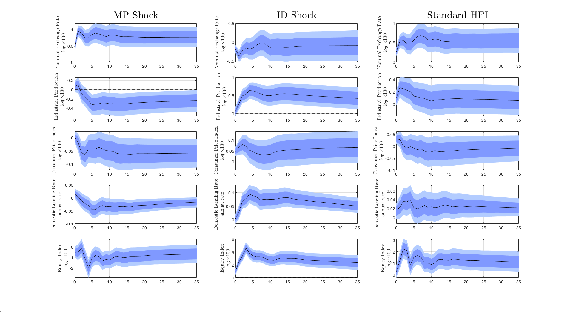
(a) Advanced Economies

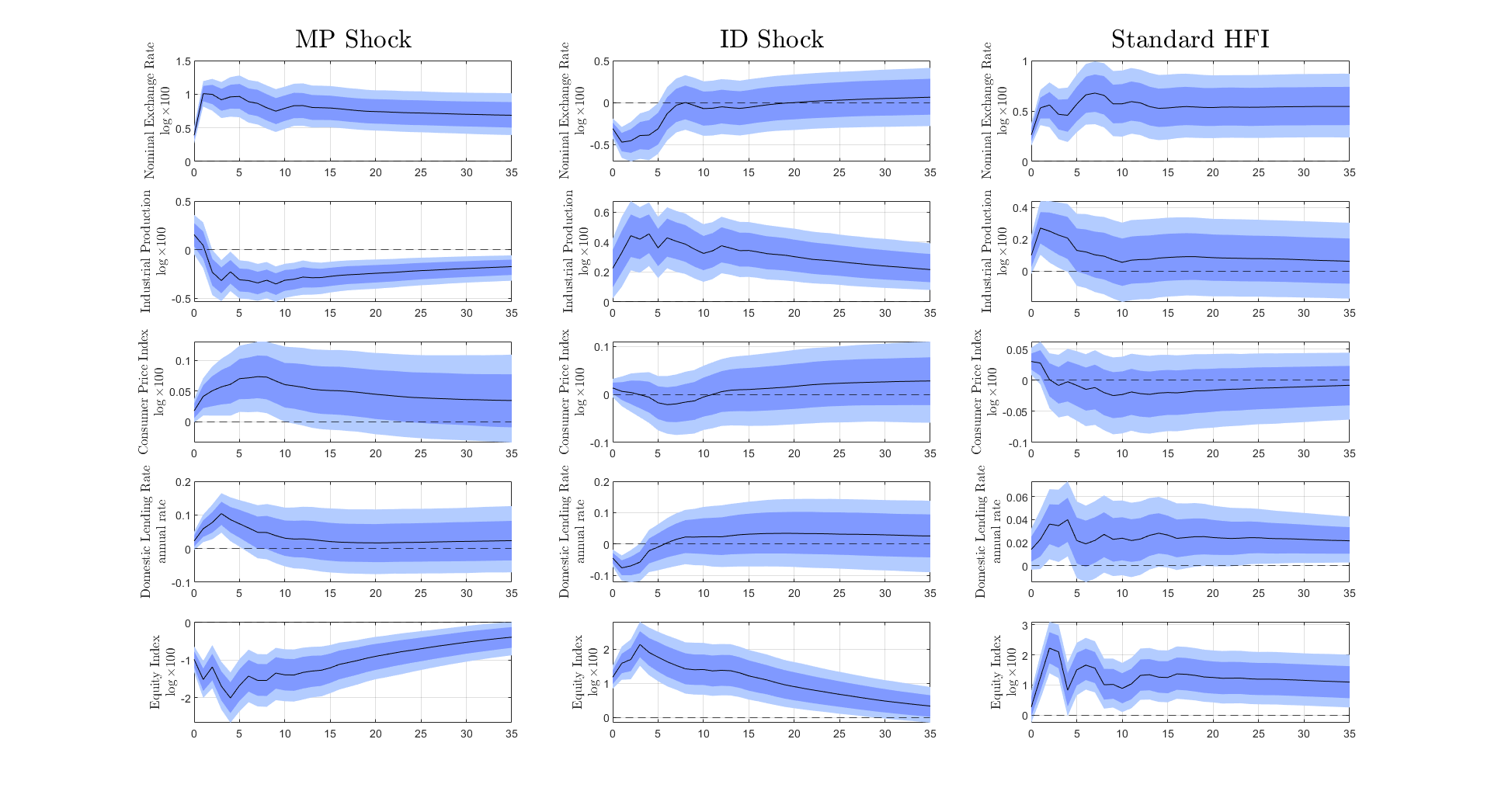
(b) Emerging Market Economies

Note: The black solid line represents the median impulse response function. The dark shaded area represents the 16 and 84 percentiles. The light shaded are represents the 5 and 95 percentiles. Figure 2(a) on the left presents the results for the panel of “Advanced Economies” comprised of: Australia, Canada, France, Iceland, Italy, Japan, South Korea, The Netherlands and Sweden. Figure 2(b) presents the results for the panel of “Emerging Market Economies” comprised of: Brazil, Chile, Colombia, Hungary, Indonesia, Mexico, Peru, Philippines and South Africa. Each figure is comprised of 15 sub-figures ordered in five rows and three columns. Every row represents a different variable: (i) nominal exchange rate, (ii) industrial production index, (iii) consumer price index, (iv) lending rate, (v) equity index. The first column presents the results for the MP or “Pure US Monetary Policy” shock, the middle column presents the results for the ID or “Information Disclosure” shock, and the last column presents the results for the interest rate composite high frequency surprise or “Standard HFI”. In the text, when referring to Panel $(i,j)$, $i$ refers to the row and $j$ to the column of the figure.

To summarize, by introducing an identification scheme which deconstruct US interest rates movements into two different FOMC shocks, I am able to show that an increase in US interest rates has completely different international spillovers depending on the underlying economic shock. While a pure monetary policy shock leads to conventional results, an information disclosure shock leads to an economic expansion, an exchange rate appreciation and looser financial conditions. Moreover, I argued that following the “Standard HFI” strategy underestimates the spillovers of a US monetary policy shock and leads to atypical dynamics, such as an expansion of industrial production and equity indexes. Lastly, I showed that these results are present for both the sub-samples of Advanced and Emerging Market economies with only minor caveats.

4 Additional Results & Robustness Checks

This section presents additional results and robustness checks that complement and support the findings presented in Section 3. First, I show that the main results are also present using local projection techniques a la Jordà [2005] to estimate impulse response functions. Second, I show that the main results are robust when using different ordering identification assumptions between the two FOMC shocks. Third, I show that the main results are robust to using different approaches to deal with the non-uniqueness problem inherent to the sign-restriction identification strategy. Lastly, I briefly describe potential sources of quantitatively heterogeneity in the spillovers of the two FOMC shocks.

Alternative model specifications. I start by showing that the main results presented in Section 3 are robust to estimating the impulse response functions to the two FOMC shocks using local projection techniques a la Jordà [2005]. We estimate the following two empirical specifications.

$$y_{i,t+h}=\beta^{MP}_{h}i^{\text{MP}}_{t}+\beta^{ID}_{h}i^{\text{ID}}_{t}+\sum^{J_{y}}_{j=1}\delta^{j}_{i}y_{i,t-j}+\sum^{J_{x}}_{j=1}\alpha^{j}_{i}x_{i,t-j}+\sum^{J_{i}}_{j=1}\left(\phi^{j}_{i}i^{\text{MP}}_{t-j}+\varphi^{j}_{i}i^{\text{ID}}_{t-j}\right)+\epsilon_{i,t}$$ (1)

$$y_{i,t+h}=\beta^{MP}_{h}i^{\text{MP}}_{t}+\beta^{ID}_{h}i^{\text{ID}}_{t}+\sum^{J_{y}}_{j=1}\delta^{j}_{i}y_{i,t-j}+\sum^{J_{x}}_{j=1}\alpha^{j}_{i}x_{i,t-j}+\sum^{J_{i}}_{j=1}\left(\phi^{j}_{i}i^{\text{MP}}_{t-j}+\varphi^{j}_{i}i^{\text{ID}}_{t-j}\right)+\Gamma_{i}+\Gamma_{i,t}+\epsilon_{i,t}$$ (2)

The first empirical specification in Equation 1, which I label “Pooled Specification”, measures outcome variable $y_{i,t+h}$ from country $i$’s at time horizon of $h$ months from date $t$. Coefficients $\beta^{MP}_{h}$ and $\beta^{ID}_{h}$ give the impulse response of outcome variable $y$ at horizon $h$ of a pure monetary policy (MP) and of an information disclosure (ID) shock, respectively. The specification includes $J_{y}$ lags of the outcome variable, $y_{i}$, $J_{x}$ lags of the other “country specific” variables $x_{i}$ and $J_{i}$ lags of the FOMC shocks. I select the number of lags by computing the Schwarz’s Bayesian information criterion (SBIC) selection statistic for each country separately. I set $J_{y}=J_{x}$ equal to 1 as it is the optimal number of lags according to the SBIC statistic for all but one country, and I choose $J_{i}=2$. I also estimate the “Pooled Specification” using the “Standard HFI” by replacing $i^{MP}_{t}$ and $i^{ID}_{t}$ with the high-frequency surprises of the policy interest rate and the S&P 500. The second specification, presented in Equation 2 includes country specific fixed effects given by $\Gamma_{c}$ and includes a linear time trend given by $\Gamma_{i,t}$. The final specification, in Equation 2 is consistent with the specification estimated by Ilzetzki and Jin [2021]. The standard errors are clustered at the country and time level, which control for the fact that all countries are hit by the FOMC shocks simultaneously.

Figures 6, 7 and 8 in Appendix C show that the findings in Section 3 are robust to estimating the impulse response functions using local projection techniques under the “Pooled Specification”, with country fixed effects and with country fixed effects plus a time trend specification. First, by comparing the estimated dynamics on the first and second columns of these figures, it is clear that under a local projection methodology the two FOMC shocks lead to opposite spillovers on the rest of the world. On the one hand, a MP shock lead to the conventional results of a drop in industrial output, a persistent nominal exchange rate depreciation and tighter financial conditions shown by higher lending rates and a drop in the equity index. On the other hand, an ID shock leads to a nominal exchange rate appreciation, a persistent increase in the industrial production index and an increase in the equity index. Results are also quantitatively close to those presented in Section 3. The last column of these figures shows that the estimated impulse response functions under the “Standard HFI” strategy lead to an average of the dynamics presented in the first two columns which yield atypical dynamics. These atypical dynamics, particularly the expansion of industrial output and the increase in the equity index, provide further evidence that the systematic disclosure of information around FOMC meetings may bias the identification and quantification of the impact of international spillovers of US monetary policy shocks.

Additionally, I show that the main results are robust to relaxing the assumption of homogeneous dynamic coefficients across countries. An alternative way to estimate panel VAR models is to use the “mean group estimator” presented in Pesaran and Smith [1995]. Under this framework it is assumed that the $N$ countries of the model are characterised by heterogeneous dynamic coefficients, but that these coefficients are random processes sharing a common mean. Therefore, the parameters of interest are the average, or mean effects of the group. Carrying out the same assumption for the residual variance-covariance matrix, namely that it is heterogeneous across countries but is characterised by a common mean, then a single and homogeneous model is estimated for all the countries.^, Figure 9 in Appendix C shows the impulse response functions of the mean group estimator and compares them with the main results. Overall, the impulse response functions of both methods are quantitatively and qualitatively inline: MP and ID shocks lead to qualitatively opposite dynamics and the “Standard HFI” approach leads to the atypical dynamics an expansion in the industrial production and equity indexes. I interpret this result as supporting evidence of the main results presented in Section 3.

Alternative shock ordering. The benchmark specification sets a specific order between the two FOMC shocks inside the vector of variables $m_{t}$, with the MP shock ordered first and the ID shock ordered second. While by construction the two FOMC shocks are orthogonal to each other, introducing them into the SVAR model may lead to spurious correlations due to the finite sample and the imposition of ordering strategies. To test the robustness of the benchmark results I re-estimate the impulse response functions using two alternative specifications of vector $m_{t}$: (i) ordering the ID shock first and the MP shock second, and by estimating the impulse response functions introducing one FOMC shock at a time. Figures 12 and 13 in Appendix C show that the main results are robust both qualitatively and quantitatively to re-ordering the two FOMC shocks, i.e. $m_{t}=[i^{ID}_{t},i^{MP}_{t}]$; and to estimating the model by introducing these shocks one at a time, i.e. estimating the impulse response functions with only one shock at a time with $m_{t}=[i^{MP}_{t}]$ and $m_{t}=[i^{ID}_{t}]$, separately, one at a time.

Alternative approach to solving non-uniqueness in sign-restrictions. The benchmark specification identifies the two FOMC shocks by choosing the median rotational angle that satisfies the sign restriction conditions. I show that the main results are robust to using different approaches to deal with the non-uniqueness problem of sign restrictions.

First, I pin down the recovery of the two FOMC shocks by using an external moment condition as in Jarociński [2022]. I compute the ratio of the variance of the MP shock to the variance of the total high-frequency surprise of the interest rate around FOMC meetings when following the “poor man’s sign restriction” approach. As presented in Jarociński and Karadi [2020], in the “poor man’s” approach each central bank announcement is classified as conveying a MP or ID shock depending on the sign of the co-movement of the high-frequency surprises. Following this approach the ratio of the variance MP shock to the variance of the high-frequency surprise of the interest rate is 0.88. Figure 14 in Appendix C presents the impulse response functions using this alternative decomposition of MP and ID shocks. Overall, results are qualitatively in line with the main results presented in Section 3 with only minor quantitative differences.^,

Second, I show that results are robust to using a uniform prior over the space of rotational angles that satisfy the sign restriction conditions (see Rubio-Ramirez et al. [2010] and Jarociński and Karadi [2020]). As argued in Section 2, the sign restriction conditions only provide set identification, i.e., conditionally on each draw of the VAR parameters there are multiple values of shocks and impulse responses that are consistent with the restrictions. When computing uncertainty bounds we take all these values into account weighting them according to the uniform prior on the rotation angles. Figure 17 in Appendix C shows the resulting impulse response functions which are quantitatively and qualitatively in line with the results presented in Section 3. Imposing a uniform prior over the space of acceptable rotations smooths out the median response and slightly increases the confidence intervals. Nevertheless, a MP and ID shock lead to opposite dynamics which are significantly different from each other and from zero. To provide intuition behind this result Figure 18 in Appendix C plots the median impulse response functions across the 99 different percentiles of acceptable rotational angles, $p=0.1,\ldots,0.99$. On the one hand, across all rotational angles, a MP shock causes an exchange rate depreciation and a drop in industrial production. On the other hand, across all rotational angles, a ID shock causes an exchange rate appreciation and an expansion of industrial production. However, the distribution of impulse response functions seem to be skewed. The top decile angles lead to dynamics close to the ones arising from the median angle than the bottom decile angles. All in all, considering alternative rotational angles which satisfy the sign restriction conditions yield results quantitatively and qualitatively in line with those presented in Section 3.

Additional evidence from alternative identification strategies. I provide supporting evidence of informational effects biasing the standard high-frequency approach by considering alternative identification strategies proposed by the literature. We consider the identification strategies proposed by Miranda-Agrippino and Ricco [2021] and Bauer and Swanson [2022]. These alternative identification strategies purge the high-frequency surprises of interest rates around FOMC of information effects by orthogonalizing from variables in the information set of the FOMC and/or from the public.

I begin by showing that estimating the international spillovers of US monetary policy using un-cleansed or un-orthogonalized shocks leads to the atypical dynamics presented in Section 3. To do this I estimate the impulse response functions of the un-orthogonalized and orthogonalized shocks constructed by Bauer and Swanson [2022]. Figure 19 in Appendix D presents this comparison. On the left column, the un-orthogonalized shock leads to a atypical dynamics, such as a non-depreciation on impact of the exchange rate and a mild expansion of the industrial production and equity indexes. On the right column, the orthogonalized shocks lead to a significant depreciation on impact which is persistent across time, and a significant drop in both the industrial production and equity index. Thus, the un-cleansed shocks lead to dynamics similar to those arising from following the “Standard HFI” strategy used in Section 3. Additionally, using a monetary policy shock purged of information effects leads to results similar to those estimated for the MP shock in Section 3.

Lastly, I compare the impulse response functions of the MP shock in this paper, with those arising from monetary policy shocks proposed by these alternative strategies. Figure 20 in Appendix D presents the result of this exercise. The first conclusion arising from this figure is that the atypical dynamics found in the literature are not present when controlling for informational effects around FOMC meetings. The second conclusion arising from this figure is that identification strategies that control for informational effects yield both quantitatively and qualitatively similar impulse response functions. I interpret these results as supporting evidence that pure monetary policy shocks still yield to the conventional results found by a previous literature and that not controlling for informational effects lead to biased estimates and atypical dynamics.

Potential sources of quantitative heterogeneity. In Appendix E I describe two potential sources of quantitatively heterogeneity in the international impact of US interest rates: (i) countries’ exchange rate regimes and (ii) countries’ reliance on the export of commodity goods. I also briefly comment how previous literature has theorized that these country characteristics may influence the quantitative impact of the spillovers of US interest rates and describe my results. The results of Section 3 are present across all the different sub-samples. In terms of exchange rate regimes, countries with managed exchange rate regimes exhibit relatively smaller impact of FOMC shocks (see Figures 21 to 24 in Appendix E). In terms of the relative importance of commodity goods in export bundles, countries with a higher dependence of commodity goods exhibit smaller quantitative impacts of FOMC shocks (see 26 and 27 in Appendix E).

5 Conclusion

In this paper I have argued that the international spillovers of a US interest rates hike depend critically on the underlying structural shock that causes the tightening. Using the identification strategy proposed by Jarociński and Karadi [2020], I deconstruct FOMC shocks into a pure US monetary policy (MP) shock and an information disclosure (ID) shock. Introducing these FOMC shocks into a SVAR model with both Advanced and Emerging Market economies I find that the two shocks lead to qualitatively opposite spillovers. On the one hand, a MP shock leads to a nominal exchange rate depreciation, a persistent drop in industrial output and overall tighter financial conditions. On the other hand, a ID shock leads to a short lived exchange rate appreciation, a persistent expansion in industrial output and overall looser financial conditions.

Furthermore, I argue that following the standard high-frequency identification of US monetary policy leads to atypical spillover dynamics as it does not control for the systematic disclosure of information about the state of the US economy around FOMC announcements. I show that this identification strategy leads to impulse response functions which are an average of those resulting from the MP and ID shocks. In particular, under this identification strategy, a US interest rate tightening leads to a significant expansion of industrial production and equity indexes. Moreover, by not controlling for the disclosure of information, this identification strategy introduces an attenuation bias in terms of the quantitative impact US monetary policy shocks on the variables which do not show atypical dynamics.

Lastly, I show that the main results are robust to a battery of different model and sample specifications. Results hold when considering Advanced and Emerging Market economies separately, when estimating impulse response functions using local projection methodologies, and when estimating the model in sub-samples of countries with different exchange rate regimes and different exposures to commodity markets.

Acknowledgements:

I owe an unsustainable debt of gratitude to Giorgio Primiceri for his guidance and advice. I would also like to thank the comments by two anonymous referees, Martin Eichenbaum, Matt Rognlie, Guido Lorenzoni and Larry Christiano. I would like to thank the Monetary and Fiscal History of Latin America project of the Becker Friedman Institute for their generous financial support. Particularly, I would like to thank Edward R. Allen, for supporting my research. I would like to thank the attendees of Northwestern University’s macro lunch seminar, Javier Garcia Cicco, Husnu Dalgic and Yong Cai. Susan Belles provided helpful comments.

Appendix A Data Details

In this section of the appendix I provide additional details on the construction of the sample used across the paper. The source of the macroeconomic and financial data used for the construction of the variables in the benchmark variable specification is the IMF’s “International Financial Statistics”.

First, the benchmark specification is comprised of five variables:

1. Nominal Exchange Rate

2. Industrial Production index

3. Consumer Price Index

4. Lending Rate

5. Equity Index

Next, I present additional details for the construction of each of the variables

• Nominal Exchange Rate: The variable’s full name at the IMF IFS data set is “Exchange Rates, National Currency Per U.S. Dollar, Period Average, Rate”.

• Industrial Production Index: In order to construct countries’ “Industrial Production Index” I rely on three variables of the IMF IFS’ dataset:

  • Economic Activity, Industrial Production, Index

  • Economic Activity, Industrial Production, Seasonally Adjusted, Index

  • Economic Activity, Industrial Production, Manufacturing, Index

  Ideally, I would construct the variable “Industrial Production Index” by choosing only one of the variables mentioned above. However, this is impossible as countries do not report to the IMF all three of these variables for our time sample, rey 2004 to December 2016. For instance, Peru provides neither the “Economic Activity, Industrial Production, Index” nor the “Economic Activity, Industrial Production, Seasonally Adjusted, Index”, but does provide the “Economic Activity, Industrial Production, Manufacturing, Index”. Visiting Peru’s Central Bank statistics website, there is no “Industrial Production Index”, but there is an “Industrial Production, Manufacturing Index”, which coincides with the variable reported as “Economic Activity, Industrial Production, Manufacturing, Index” to the IMF.

  In order to deal with this, I establish the following priority between the three IMF IFS variables: (i) “Economic Activity, Industrial Production, Seasonally Adjusted, Index” (ii) “Economic Activity, Industrial Production, Index”, (iii) “Economic Activity, Industrial Production, Manufacturing, Index”. Table 2 below presents the IMF IFS variable used for each country.

  Table 2: Construction of Industrial Production Index

  Emerging Markets
  Brazil	Economic Activity, Industrial Production, Seasonally Adjusted, Index
  Chile	Economic Activity, Industrial Production, Seasonally Adjusted, Index
  Colombia	Economic Activity, Industrial Production, Seasonally Adjusted, Index
  Hungary	Economic Activity, Industrial Production, Seasonally Adjusted, Index
  Indonesia	Economic Activity, Industrial Production, Manufacturing, Index
  Mexico	Economic Activity, Industrial Production, Seasonally Adjusted, Index
  Peru	Economic Activity, Industrial Production, Manufacturing, Index
  Philippines	Economic Activity, Industrial Production, Manufacturing, Index
  South Africa	Economic Activity, Industrial Production, Manufacturing, Index
  Advanced Economies
  Australia	Economic Activity, Industrial Production, Seasonally Adjusted, Index
  Canada	Economic Activity, Industrial Production, Seasonally Adjusted, Index
  France	Economic Activity, Industrial Production, Seasonally Adjusted, Index
  Iceland	Economic Activity, Industrial Production, Seasonally Adjusted, Index
  Italy	Economic Activity, Industrial Production, Seasonally Adjusted, Index
  Japan	Economic Activity, Industrial Production, Seasonally Adjusted, Index
  South Korea	Economic Activity, Industrial Production, Seasonally Adjusted, Index
  The Netherlands	Economic Activity, Industrial Production, Seasonally Adjusted, Index
  Sweden	Economic Activity, Industrial Production, Seasonally Adjusted, Index

  I believe that every one of the three variables considered reflects the actual industrial production index. From Table 2, it is clear that when “Economic Activity, Industrial Production, Seasonally Adjusted, Index” is not available, the non-seasonally adjusted is also not available. Also, the fact that results are significant for Emerging Market Economies and Advanced Economies separately, see Figures 2(b) and 2(a) respectively, suggest that the paper’s main results are not driven by the choice of variable. This conclusion also follows from the fact that the paper’s main results are robust to the several sub-sample exercises carried out in Section 4.

• Consumer Price Index: Data for all countries except Australia is constructed using the variable “Prices, Consumer Price Index, All items, Index” from IMF IFS data set. Australia does not report a monthly CPI series to the IMF-IFS data set. Furthermore, the Australian Bureau of Statistics provides only quarterly data on their consumer price index. Thus, for the case of Australia I proxy the monthly consumer price index by using the “Prices, Producer Price Index, All Commodities, Index”. Once again, given that the paper’s main results are robust to the different exercises that partition the sample, I believe that using this proxy variable does not guide any of the of the results presented in the paper.

• Lending Rate: For all countries except France, the Netherlands and Sweden I use the IMF-IFS’ “Monetary and Financial Accounts, Interest Rates, Other Depository Corporations Rates, Lending Rates, Lending Rate, Percent per Annum” variable. For France, the Netherlands and Sweden I use the OECD Stats, “Monthly Monetary and Financial Statistics (MEI)” dataset variable “Short-term interest rates, Per cent per annum”.

• Equity Index: In order to construct countries’ “Equity Index” I rely on two variables of the IMF IFS’ dataset:

  • Monetary and Financial Accounts, Financial Market Prices, Equities, Index

  • Monetary and Financial Accounts, Financial Market Prices, Equities, End of Period, Index

  I establish a priority: (i) “Monetary and Financial Accounts, Financial Market Prices, Equities, Index” (ii) “Monetary and Financial Accounts, Financial Market Prices, Equities, End of Period, Index”. Again, the data coverage is not complete for all countries for the full sample period of January 2004 to December 2016. Table 3 presents index used for every country.

  Table 3: Construction of Equity Index

  Emerging Markets
  Brazil	Equities, End of Period, Index
  Chile	Equities, Index
  Colombia	Equities, End of Period, Index
  Indonesia	Equities, Index
  Hungary	Equities, Index
  Mexico	Equities, End of Period, Index
  Peru	Equities, End of Period, Index
  Philippines	Equities, Index
  South Africa	Equities, Index
  Advanced Economies
  Australia	Equities, End of Period, Index
  Canada	Equities, Index
  France	Equities, Index
  Iceland	Equities, Index
  Italy	Equities, Index
  Japan	Equities, Index
  South Korea	Equities, Index
  the Netherlands	Equities, Index
  Sweden	Equities, Index

Appendix B Model Details

In this section of the appendix I provide additional details on the panel SVAR model and the identification strategy described in Section 2. Section B.1 presents details on the panel SVAR model while Section B.2 presents additional technical details on the recovery of structural shocks.

B.1 Panel SVAR Model

In this section of the appendix I provide additional details on the estimation of the Structural VAR model presented in Section 2. In its most general form, a panel SVAR model comprises of N countries or units, $n$ endogenous variables, $p$ lagged values and $T$ time periods. The pooled panel SVAR model can be written as

$$\begin{pmatrix}y_{1,t}\\ y_{2,t}\\ \vdots\\ y_{N,t}\end{pmatrix} =C+\begin{pmatrix}A^{1}\quad 0\quad\cdots\quad 0\\ 0\quad A^{1}\quad\cdots\quad 0\\ \vdots\quad\vdots\quad\ddots\quad\vdots\\ 0\quad 0\quad\cdots\quad A^{1}\end{pmatrix}\begin{pmatrix}y_{1,t-1}\\ y_{2,t-1}\\ \vdots\\ y_{N,t-1}\end{pmatrix}+\cdots$$

$$+\begin{pmatrix}A^{p}\quad 0\quad\cdots\quad 0\\ 0\quad A^{p}\quad\cdots\quad 0\\ \vdots\quad\vdots\quad\ddots\quad\vdots\\ 0\quad 0\quad\cdots\quad A^{p}\end{pmatrix}\begin{pmatrix}y_{1,t-p}\\ y_{2,t-p}\\ \vdots\\ y_{N,t-p}\end{pmatrix}+\begin{pmatrix}\epsilon_{1,t}\\ \epsilon_{2,t}\\ \vdots\\ \epsilon_{N,t}\end{pmatrix}$$

where $y_{i,t}$ denotes an $n\times 1$ vector of $n$ endogenous variables of country $i$ at time $t$ and $A^{j}$ is an $n\times n$ matrix of coefficients providing the response of country $i$ to the $j^{th}$ lag at period $t$. Note that by assuming that $A^{j}_{1}=A^{j}_{n}=A^{j}$ for $j=1,\ldots,n$ implies the assumption that the estimated coefficients are common across countries. $C$ is a $Nn\times 1$ vector of constant terms which are also assumed to be common across countries. Lastly, $\epsilon_{i,t}$ is an $n\times 1$ vector of residuals for the variables of country $i$, such that

$$\epsilon_{i,t}\sim\mathcal{N}\left(0,\Sigma_{ii,t}\right)$$

with

$$\epsilon_{ii,t} =\mathbb{E}\left(\epsilon_{i,t}\epsilon_{i,t}^{\prime}\right)=\Sigma_{c}\quad\forall i$$

$$\epsilon_{ij,t} =\mathbb{E}\left(\epsilon_{i,t}\epsilon_{j,t}^{\prime}\right)=0\quad\text{for }i\neq j$$

The last two equations imply that, as for the model’s auto-regressive coefficients, the innovation’s variance is equal across countries.

The model described by Equation B.1 is estimated using Bayesian methods. In order to carry out the estimation of this model I first re-write the model. In particular, the model can be reformulated in compact form as

$$\underbrace{\begin{pmatrix}y_{1,t}^{\prime}\\ y_{2,t}^{\prime}\\ \vdots\\ y_{N,t}^{\prime}\end{pmatrix}}_{Y_{t},\quad N\times n} =\underbrace{\begin{pmatrix}y_{1,t-1}^{\prime}\ldots y_{1,t-p}^{\prime}\\ y_{2,t-1}^{\prime}\ldots y_{2,t-p}^{\prime}\\ \vdots\ddots\vdots\\ y_{N,t-1}^{\prime}\ldots y_{N,t-p}^{\prime}\end{pmatrix}}_{\mathcal{B},\quad N\times np}\underbrace{\begin{pmatrix}\left(A^{1}\right)^{\prime}\\ \left(A^{2}\right)^{\prime}\\ \vdots\\ \left(A^{N}\right)^{\prime}\end{pmatrix}}_{X_{t},\quad np\times n}+\underbrace{\begin{pmatrix}\epsilon_{1,t}^{\prime}\\ \epsilon_{2,t}^{\prime}\\ \vdots\\ \epsilon_{N,t}^{\prime}\end{pmatrix}}_{\mathcal{E}_{t},\quad N\times n}$$ (4)

or

$$Y_{t}=X_{t}\mathcal{B}+\mathcal{E}_{t}$$ (5)

Even more, the model can be written in vectorised form by stacking over the $T$ time periods

$$\underbrace{vec\left(Y\right)}_{NnT\times 1}=\underbrace{\left(I_{n}\otimes X\right)}_{NnT\times nnp}\quad\underbrace{vec\left(\mathcal{B}\right)}_{nnp\times 1}\quad+\quad\underbrace{vec\left(\mathcal{E}\right)}_{NnT\times 1}$$ (6)

or

$$y=\bar{X}\beta+\epsilon$$ (7)

where $\epsilon\sim\mathcal{N}\left(0,\bar{\Sigma}\right)$, with $\bar{\Sigma}=\Sigma_{c}\otimes I_{NT}$.

The model described above is just a conventional VAR model. Thus, the traditional Normal-Wishart identification strategy is carried out to estimate it. The likelihood function is given by

$$f\left(y|\bar{X}\right)\propto|\bar{\Sigma}|^{-\frac{1}{2}}\exp\left(-\frac{1}{2}\left(y-\bar{X}\beta\right)^{\prime}\bar{\Sigma}^{-1}\left(y-\bar{X}\beta\right)\right)$$ (8)

As for the Normal-Wishart, the prior of $\beta$ is assumed to be multivariate normal and the prior for $\Sigma_{c}$ is inverse Wishart. For further details, see Dieppe et al. [2016]. All of the panel SVAR model computations are carried out using the BEAR Toolbox version 5.1.

B.2 Identification Strategy & Shock Recovery

In this section of the appendix, I present additional details on the sign-restriction identification strategy presented in Section 2 which recovers the two FOMC structural shocks. As stated in Section 2, this identification strategy follows Jarociński and Karadi [2020] and Jarociński [2022].

The identification strategy introduced by Jarociński [2022] exploit the high-frequency surprises of multiple financial instruments to recover two distinct FOMC shocks: a pure monetary policy (MP) shock and information disclosure (ID) shock. In particular, the authors impose sign restrictions conditions on the co-movement of the high-frequency surprises of interest rates and the S&P 500 around FOMC meetings. This co-movement is informative as standard theory unambiguously predicts that a monetary policy tightening shock should lead to lower stock market valuation. This is because a monetary policy tightening decreases the present value of future dividends by increasing the discount rate and by deteriorating present and future firm’s profits and dividends. Thus, MP shocks are identified as those innovations that produce a negative co-movement between these high-frequency financial variables. On the contrary, innovations generating a positive co-movement between interest rates and the S&P 500 correspond to ID shocks.

Figure 3 presents a scatter plot of the high-frequency surprises of interest rates and the S&P 500 around FOMC meetings.

Figure 3: Scatter Plot of Interest Rate & S&P 500 Surprises around FOMC Meetings

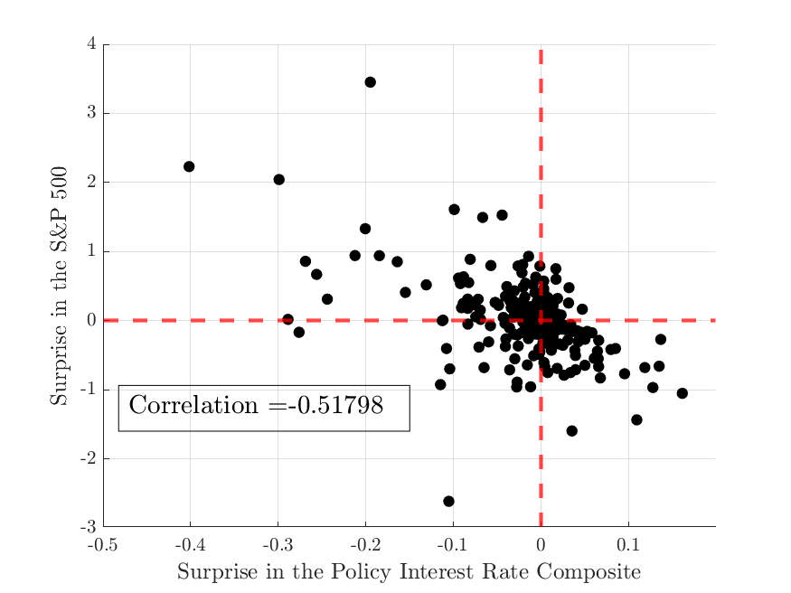
(a) 1990 - 2018

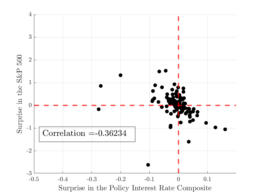
(b) 2004 - 2016

Note: The left panel presents data for the period 1990-2018, in line with the sample constructed by Jarociński [2022]. The right panel presents data for the period 2004-2016, the sample for the empirical exercises in Section 3. The high-frequency changes of the Policy Interest Rate Composite and the S&P 500 are computed using 30-minute windows around FOMC meetings. Each black filled circle represents a different FOMC meeting.

The co-movement of these high-frequency surprises is remarkably different across FOMC meetings. Although a majority of FOMC meetings exhibit a negative co-movement between the interest rates and S&P 500 surprises, a significant share of observations exhibit a positive co-movement. The authors’ way to account for the positive co-movement is to attribute it to a shock that occurs systematically at the same time the FOMC announces its policy decisions, but that is different from a standard monetary policy shock. In particular, this additional shock is the disclosure of the FOMC’s information about the present and future state of the US economy. Hence, by combining both the high-frequency surprises and imposing sign-restriction in their co-movements, the authors separately identify two structural FOMC shocks: a pure US monetary policy (MP) shock (which exhibits a negative co-movement between the interest rates and S&P high-frequency surprises) and an information disclosure (ID) shock (which exhibits a positive co-movement between the interest rates and S&P high-frequency surprises).

The high frequency surprise in the policy interest rate, $i^{Total}$, can be decomposed as

$$i^{\text{Total}}=i^{\text{MP}}+i^{\text{ID}}$$ (9)

where $i^{\text{MP}}$ is negatively correlated with the high frequency surprise of the $S\&P500$ “$s$”, and $i^{\text{ID}}$ is positively correlated with the “$s$”. As shown by Jarociński [2022], the sign restriction recovery of the structural shocks must satisfy the following decomposition

$$M=UC$$ (10)

where $U^{\prime}U$ is a diagonal matrix, $C$ takes the form of

$$C=\begin{pmatrix}1&c^{MP}<0\\ 1&c^{ID}>0\\ \end{pmatrix}$$ (11)

where $M=(i^{Total},s)$ is a $T\times 2$ matrix with $i^{Total}$ in the first column, $s$ in the second; $U=(i^{\text{MP}},i^{\text{ID}})$ is a $T\times 2$ matrix with $i^{\text{MP}}$ in the first column and $i^{\text{ID}}$ in the second column; and $T$ denoting the time length of the sample. By construction, $i^{\text{MP}}$ and $i^{\text{ID}}$ are mutually orthogonal. Matrix $C$ captures how $i^{\text{MP}}$ and $i^{\text{ID}}$ translates into financial market surprises.

The decomposition in 11 is not unique. In terms of Jarociński [2022] there is a range of rotations of matrices $U$ and $C$ that satisfy the sign restrictions $c^{MP}<0$ and $c^{ID}>0$.

The matrices $U$ and $C$ are computed as

$$U =QPD$$ (12)

$$C =D^{-1}P^{\prime}R$$ (13)

where the matrices $Q,P,D,R$ are obtained in three steps.

• Decompose matrix $M=UC$ into two orthogonal components using a QR decomposition such that

$$M =QR$$ (14)

$$Q^{\prime}Q =\begin{pmatrix}1&0\\ 0&1\\ \end{pmatrix}$$ (15)

$$R =\begin{pmatrix}r_{1,1}>0&r_{1,2}\\ 0&r_{2,2}>0\\ \end{pmatrix}$$ (16)

• Rotate these orthogonal components using the rotation matrix

  $$P =\begin{pmatrix}\cos\left(\alpha\right)&\sin\left(\alpha\right)\\ -\sin\left(\alpha\right)&\cos\left(\alpha\right)\end{pmatrix}$$ (17)

  To satisfy the sign restrictions use any angle $\alpha$ in the following range

  $$\alpha\in\left(\left(1-w\right)\times\arctan\frac{r_{1,2}}{r_{2,2}},\frac{w\times\pi}{2}\right)\qquad\text{if }r_{1,2}>0$$

  $$\alpha\in\left(0,w\times\arctan\frac{-r_{2,2}}{r_{1,2}}\right)\qquad\text{if }r_{1,2}\leq 0$$

  where $w$ is weight, between 0 and 1, scaling the rotation angle. Setting $w=0.5$ implies the median rotation angle, assumption used under the benchmark specification

• Re-scale the resulting orthogonal components with a diagonal matrix $D$ to ensure that they add up to the interest rate surprises $i^{\text{Total}}$. It is straightforward to show that

  $$D=\begin{pmatrix}r_{1,1}\cos\left(\alpha\right)&0\\ 0&r_{1,1}\sin\left(\alpha\right)\end{pmatrix}$$ (18)

Figures 4 and 5 present the time series of the high frequency surprise of the interest rate and of the two recovered structural for my benchmark specification, respectively.

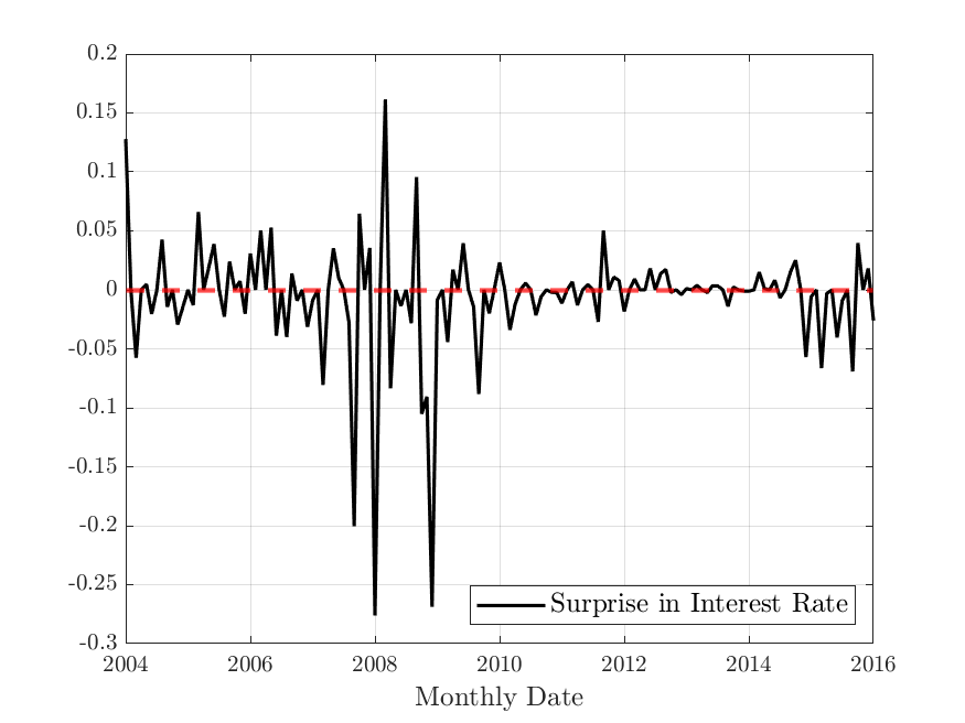
Figure 4: High-Frequency Financial Surprises around FOMC Meetings

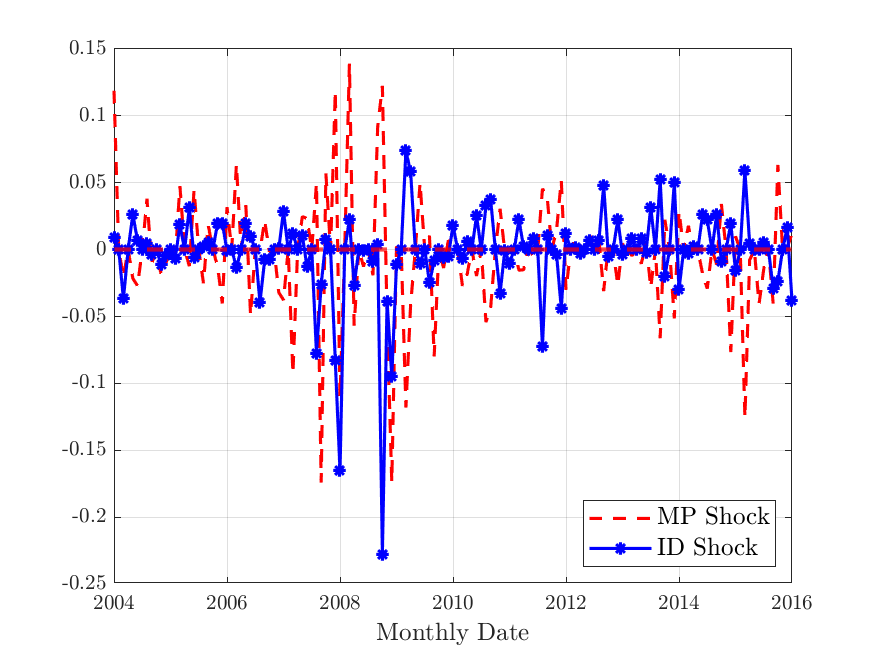
Figure 5: Structural FOMC Shocks

The first robustness check in Section 4 which proposes an alternative approach to deal with the non-uniqueness problem of sign-restriction identification follows the approach of Jarociński [2022]. In Jarociński [2022], the angle of rotation $\alpha$ of matrix $P$ is pinned down following these steps

• Construct “poor man’s sign restrictions” shocks such that

  $$i^{\text{Total}} =i^{MP}\quad\&\quad i^{\text{ID}}=0\qquad\text{if }i^{Total}\times s\leq 0$$

  $$i^{\text{Total}} =i^{ID}\quad\&\quad i^{\text{MP}}=0\qquad\text{if }i^{Total}\times s>0$$

In the data, Jarociński [2022] finds that the poor man’s monetary policy shocks account for 88% of the variance of the Federal Reserve’s total interest rate surprises, i.e,

$$\frac{var\left(i^{\text{MP}}\right)}{var\left(i^{\text{Total}}\right)}=0.88$$

To pin down the decomposition, Jarociński [2022] impose that, as in the “poor man’s sign restrictions” case, $var\left(i^{\text{MP}}\right)/var\left(i^{\text{MP}}\right)=0.88$. Additionally, Jarociński [2022] shows that the angle $\alpha$ can meets this condition can be recovered as

$$\alpha=\arccos\sqrt{\frac{var\left(i^{\text{MP}}\right)}{var\left(i^{\text{Total}}\right)}}$$ (19)

In particular, the $\alpha$ that meets this condition is set equal to $\alpha=0.8702$.

In Section 4 I carry out several robustness checks that considering different rotational angles.

Appendix C Additional Results

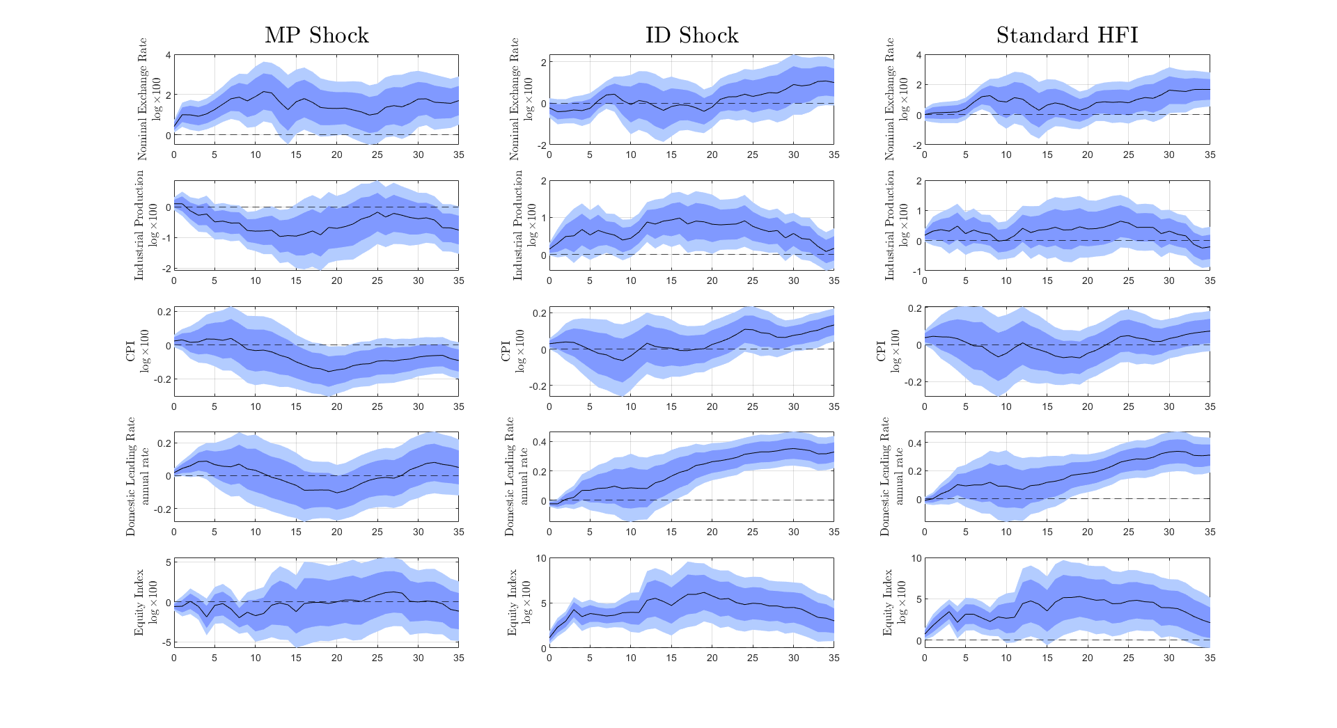
Figure 6: Local Projection Impulse Response Functions
Pooled Specification

Note: The black solid line represents the point estimate of coefficient for either one of the two FOMC shocks, or the high-frequency surprise of the policy interest rate composite. The dark shaded area represents within +/- one standard deviation, and the light shaded are represents the area within 1.65 standard deviations from the point estimate. The figure is comprised of 15 sub-figures ordered in five rows and three columns. Every row represents a different variable: (i) nominal exchange rate, (ii) industrial production index, (iii) consumer price index, (iv) lending rate, (v) equity index. The first column presents the results for the MP or “Pure US Monetary Policy” shock, the middle column presents the results for the ID or “Information Disclosure” shock, and the last column presents the results for the interest rate composite high frequency surprise or “Standard HFI”. In the text, when referring to Panel $(i,j)$, $i$ refers to the row and $j$ to the column of the figure. For each shock, I standardize the coefficients such that they represent the dynamics of a one-standard deviation shock.

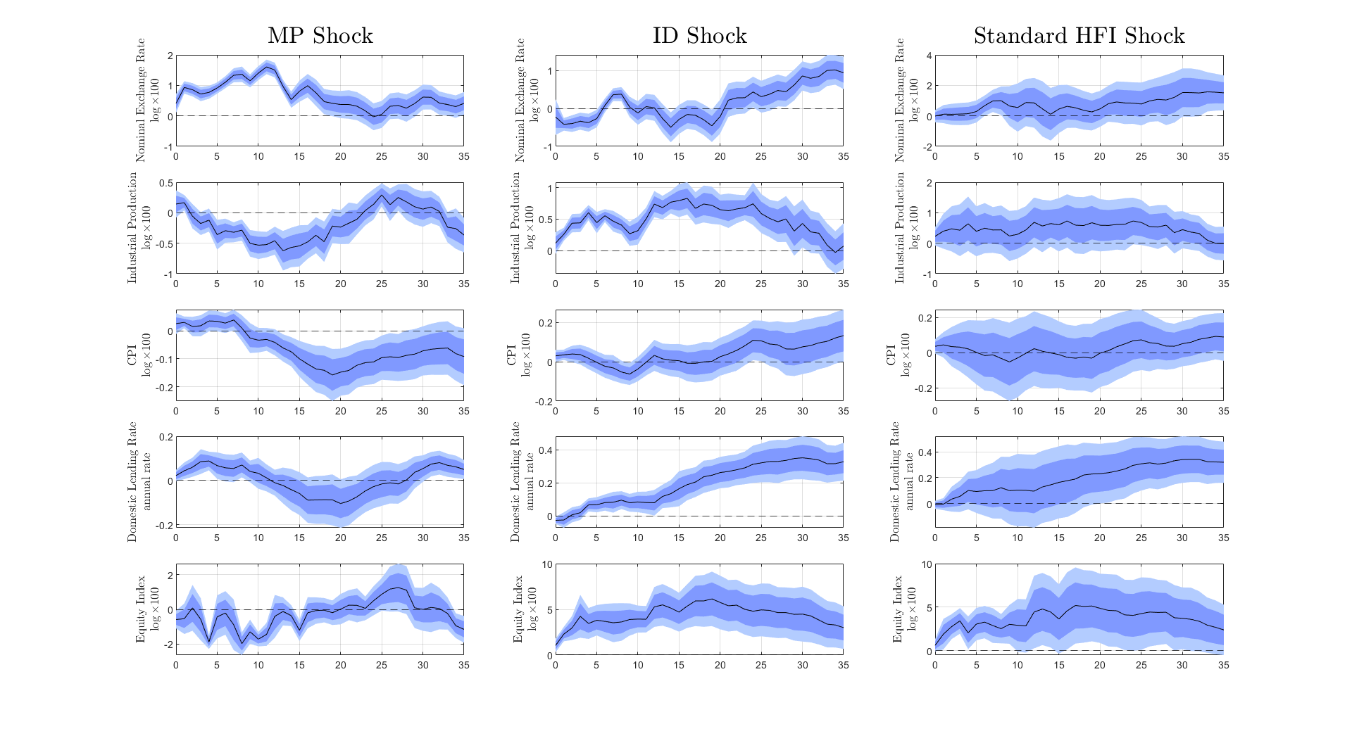
Figure 7: Local Projection Impulse Response Functions
F.E. Specification

Note: The black solid line represents the point estimate of coefficient for either one of the two FOMC shocks, or the high-frequency surprise of the policy interest rate composite. The dark shaded area represents within +/- one standard deviation, and the light shaded are represents the area within 1.65 standard deviations from the point estimate. The figure is comprised of 15 sub-figures ordered in five rows and three columns. Every row represents a different variable: (i) nominal exchange rate, (ii) industrial production index, (iii) consumer price index, (iv) lending rate, (v) equity index. The first column presents the results for the MP or “Pure US Monetary Policy” shock, the middle column presents the results for the ID or “Information Disclosure” shock, and the last column presents the results for the interest rate composite high frequency surprise or “Standard HFI”. In the text, when referring to Panel $(i,j)$, $i$ refers to the row and $j$ to the column of the figure. For each shock, I standardize the coefficients such that they represent the dynamics of a one-standard deviation shock.

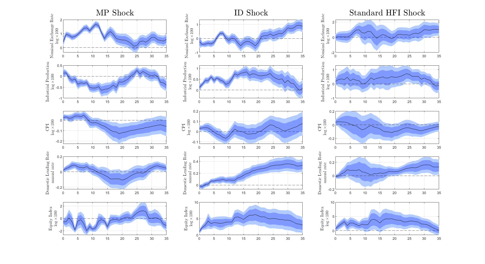
Figure 8: Local Projection Impulse Response Functions
F.E. + Time Trend Specification

Note: The black solid line represents the point estimate of coefficient for either one of the two FOMC shocks, or the high-frequency surprise of the policy interest rate composite. The dark shaded area represents within +/- one standard deviation, and the light shaded are represents the area within 1.65 standard deviations from the point estimate. The figure is comprised of 15 sub-figures ordered in five rows and three columns. Every row represents a different variable: (i) nominal exchange rate, (ii) industrial production index, (iii) consumer price index, (iv) lending rate, (v) equity index. The first column presents the results for the MP or “Pure US Monetary Policy” shock, the middle column presents the results for the ID or “Information Disclosure” shock, and the last column presents the results for the interest rate composite high frequency surprise or “Standard HFI”. In the text, when referring to Panel $(i,j)$, $i$ refers to the row and $j$ to the column of the figure. For each shock, I standardize the coefficients such that they represent the dynamics of a one-standard deviation shock.

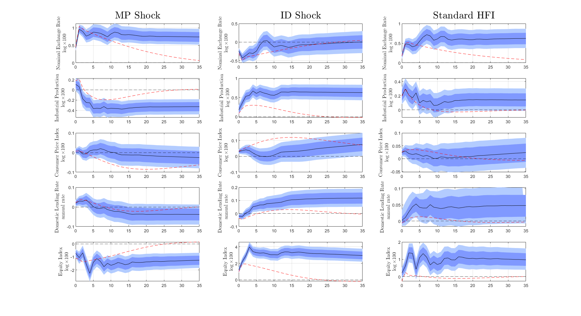
Figure 9: Impulse Response to One-Standard-Deviation Shock
Mean Group Estimator

Note: The black solid line represents the median impulse response function. The dark shaded area represents the 16 and 84 percentiles. The light shaded are represents the 5 and 95 percentiles. The red dashed line is the mean group estimator which plots the average response across countries. The figure is comprised of 15 sub-figures ordered in five rows and three columns. Every row represents a different variable: (i) the MP structural FOMC shock, (ii) the ID structural FOMC shock, (iii) nominal exchange rate, (iv) industrial production index, (v) consumer price index, (vi) lending rate, (vii) equity index. The first column presents the results for the MP or “Pure US Monetary Policy” shock, the middle column the ID or “Information Disclosure” shock and the the last column presents the results following the “Standard High Frequency” identification shock. In the text, when referring to Panel $(i,j)$, $i$ refers to the row and $j$ to the column of the figure.

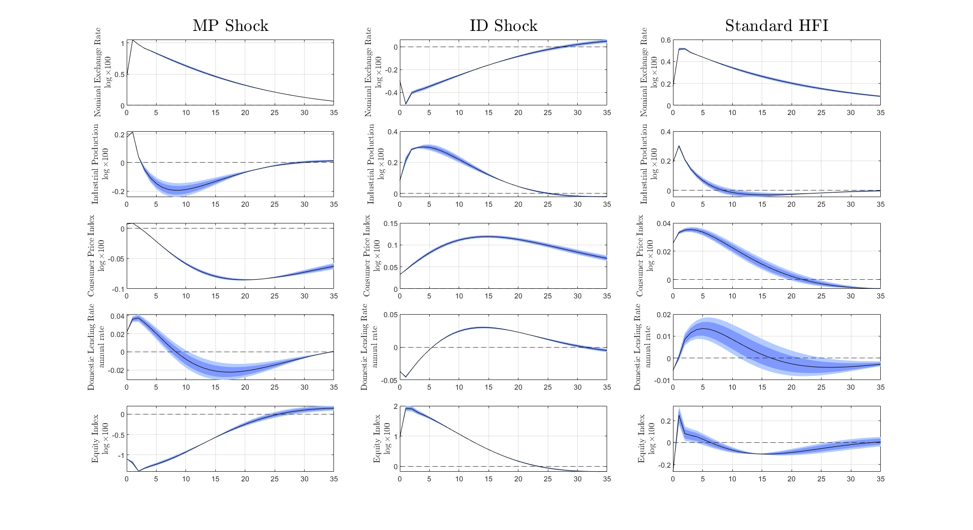
Figure 10: Impulse Response to One-Standard-Deviation Shock
Mean Group Estimator

Note: The black solid line represents the median impulse response function. The dark shaded area represents the 16 and 84 percentiles. The light shaded are represents the 5 and 95 percentiles. The figure is comprised of 15 sub-figures ordered in five rows and three columns. Every row represents a different variable: (i) the MP structural FOMC shock, (ii) the ID structural FOMC shock, (iii) nominal exchange rate, (iv) industrial production index, (v) consumer price index, (vi) lending rate, (vii) equity index. The first column presents the results for the MP or “Pure US Monetary Policy” shock, the middle column the ID or “Information Disclosure” shock and the the last column presents the results following the “Standard High Frequency” identification shock. In the text, when referring to Panel $(i,j)$, $i$ refers to the row and $j$ to the column of the figure.

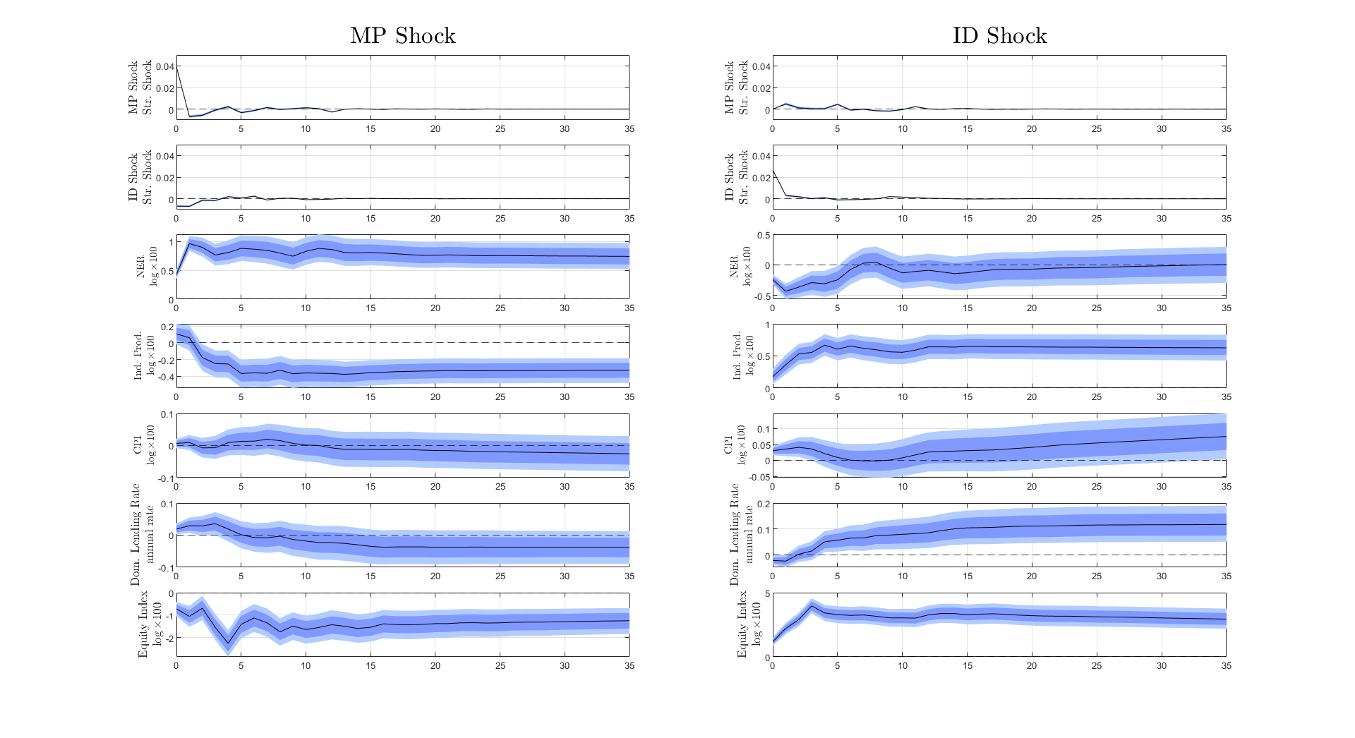
Figure 11: Impulse Response to One-Standard-Deviation Shock
All Variables

Note: The black solid line represents the median impulse response function. The dark shaded area represents the 16 and 84 percentiles. The light shaded are represents the 5 and 95 percentiles. The figure is comprised of 14 sub-figures ordered in seven rows and two columns. Every row represents a different variable: (i) the MP structural FOMC shock, (ii) the ID structural FOMC shock, (iii) nominal exchange rate, (iv) industrial production index, (v) consumer price index, (vi) lending rate, (vii) equity index. The first column presents the results for the MP or “Pure US Monetary Policy” shock, the last or right column presents the results for the ID shock. In the text, when referring to Panel $(i,j)$, $i$ refers to the row and $j$ to the column of the figure.

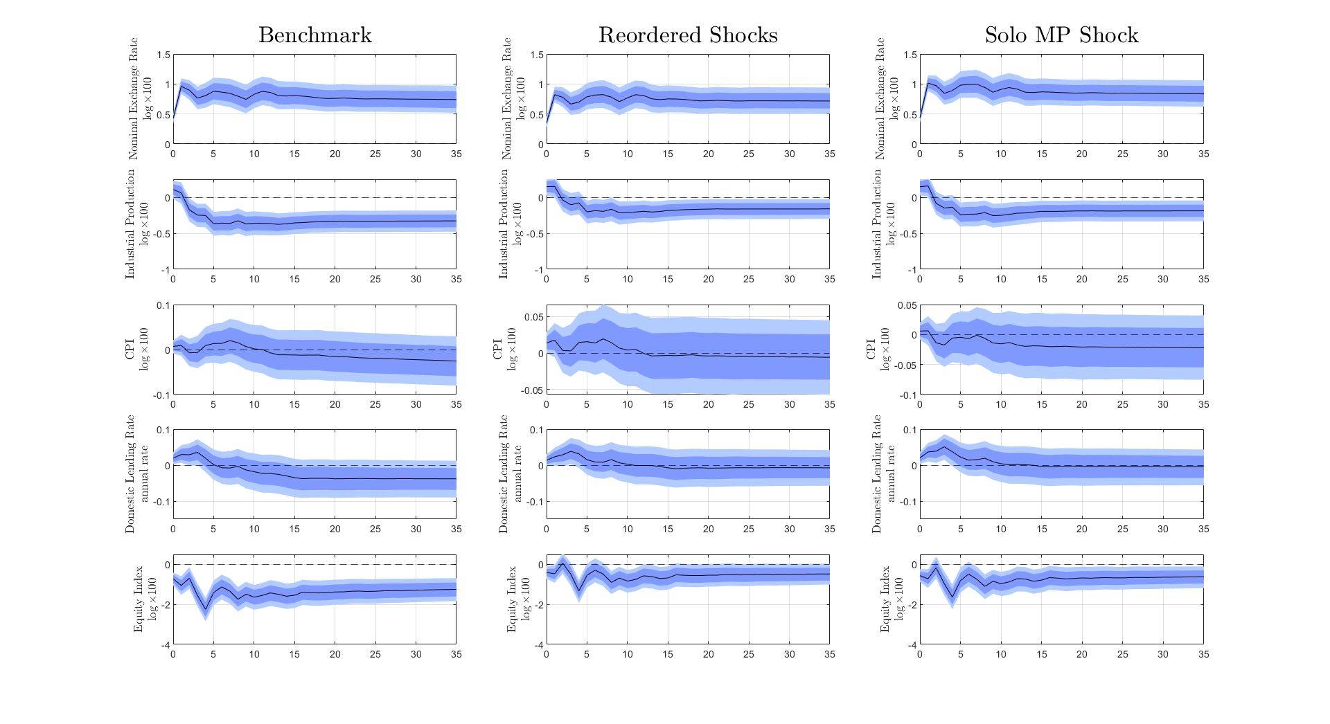
Figure 12: Impulse Response to One-Standard-Deviation Shock
MP Shock Reordering

Note: The black solid line represents the median impulse response function. The dark shaded area represents the 16 and 84 percentiles. The light shaded are represents the 5 and 95 percentiles. The figure is comprised of 15 sub-figures ordered in five rows and three columns. Every row represents a different variable: (i) the MP structural FOMC shock, (ii) the ID structural FOMC shock, (iii) nominal exchange rate, (iv) industrial production index, (v) consumer price index, (vi) lending rate, (vii) equity index. The first column presents the results for the MP shock using the benchmark specification. The middle column presents the results re-ordering the ID shock first and the MP shock second. The last column presents the results when only including the MP shock in the SVAR specification. In the text, when referring to Panel $(i,j)$, $i$ refers to the row and $j$ to the column of the figure.

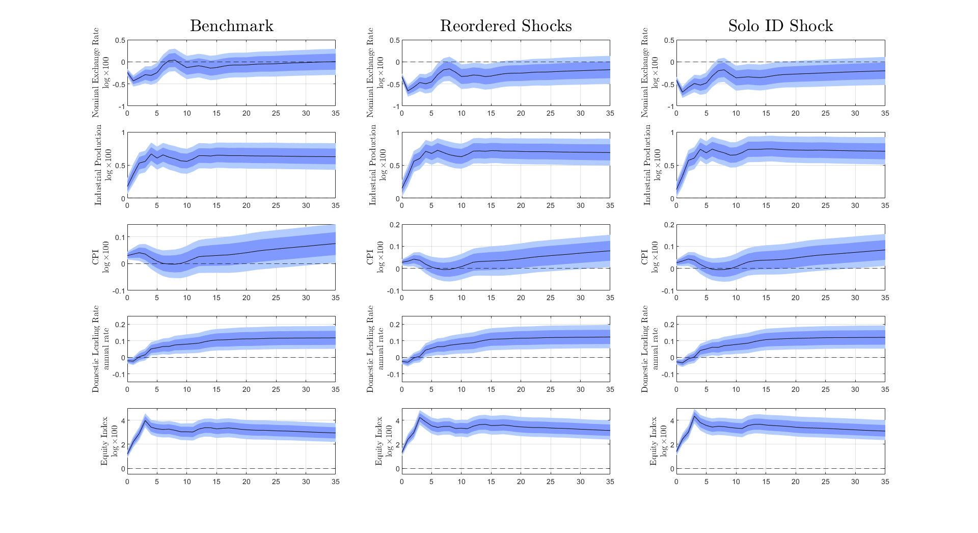
Figure 13: Impulse Response to One-Standard-Deviation Shock
ID Shock Reordering

Note: The black solid line represents the median impulse response function. The dark shaded area represents the 16 and 84 percentiles. The light shaded are represents the 5 and 95 percentiles. The figure is comprised of 15 sub-figures ordered in five rows and three columns. Every row represents a different variable: (i) the MP structural FOMC shock, (ii) the ID structural FOMC shock, (iii) nominal exchange rate, (iv) industrial production index, (v) consumer price index, (vi) lending rate, (vii) equity index. The first column presents the results for the ID shock using the benchmark specification. The middle column presents the results re-ordering the ID shock first and the MP shock second. The last column presents the results when only including the ID shock in the SVAR specification. In the text, when referring to Panel $(i,j)$, $i$ refers to the row and $j$ to the column of the figure.

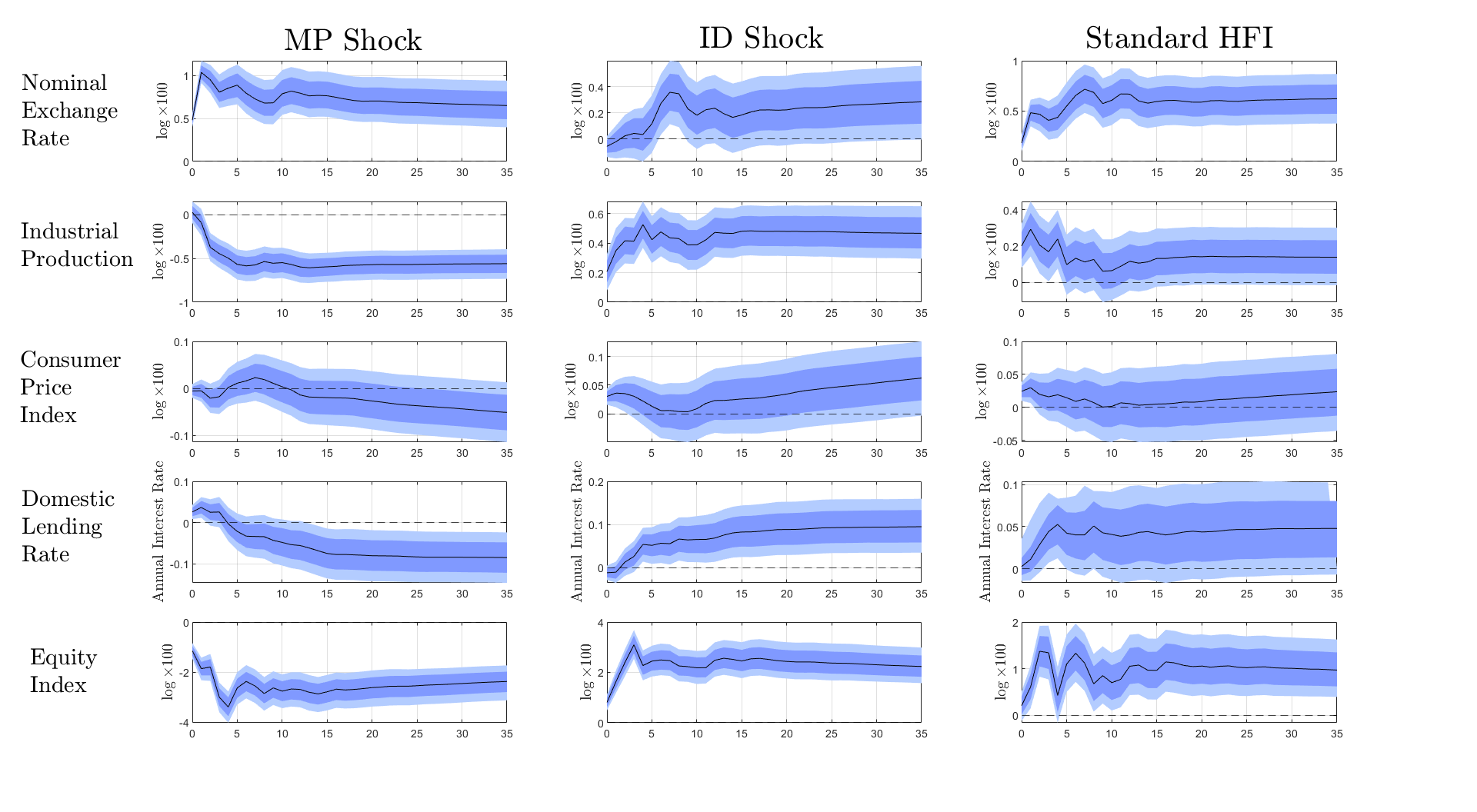
Figure 14: Impulse Response to One-Standard-Deviation Shock
External Moment Condition

Note: The black solid line represents the median impulse response function. The dark shaded area represents the 16 and 84 percentiles. The light shaded are represents the 5 and 95 percentiles. The figure is comprised of 15 sub-figures ordered in five rows and three columns. Every row represents a different variable: (i) the MP structural FOMC shock, (ii) the ID structural FOMC shock, (iii) nominal exchange rate, (iv) industrial production index, (v) consumer price index, (vi) lending rate, (vii) equity index. The first column presents the results for the MP or “Pure US Monetary Policy” shock, the middle column the ID or “Information Disclosure” shock and the the last column presents the results following the “Standard High Frequency” identification shock. In the text, when referring to Panel $(i,j)$, $i$ refers to the row and $j$ to the column of the figure.

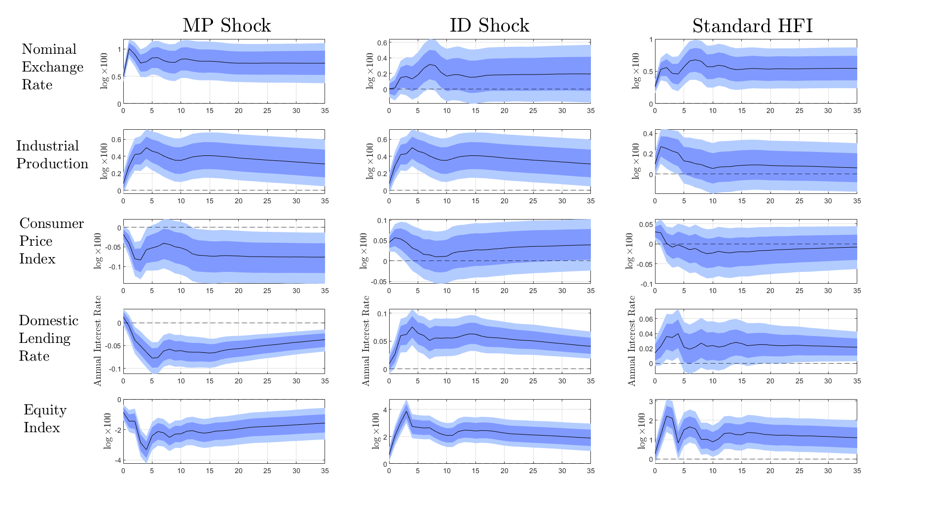
Figure 15: Impulse Response to One-Standard-Deviation Shock
Ext. Moment Condition - AE

Note: The black solid line represents the median impulse response function. The dark shaded area represents the 16 and 84 percentiles. The light shaded are represents the 5 and 95 percentiles. The figure is comprised of 15 sub-figures ordered in five rows and three columns. Every row represents a different variable: (i) the MP structural FOMC shock, (ii) the ID structural FOMC shock, (iii) nominal exchange rate, (iv) industrial production index, (v) consumer price index, (vi) lending rate, (vii) equity index. The first column presents the results for the MP or “Pure US Monetary Policy” shock, the middle column the ID or “Information Disclosure” shock and the the last column presents the results following the “Standard High Frequency” identification shock. In the text, when referring to Panel $(i,j)$, $i$ refers to the row and $j$ to the column of the figure.

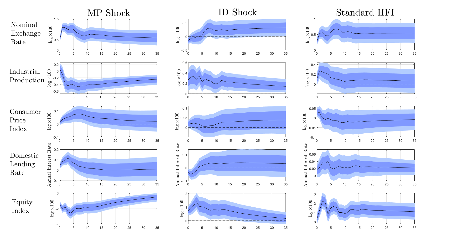
Figure 16: Impulse Response to One-Standard-Deviation Shock
Ext. Moment Condition - EM

Note: The black solid line represents the median impulse response function. The dark shaded area represents the 16 and 84 percentiles. The light shaded are represents the 5 and 95 percentiles. The figure is comprised of 15 sub-figures ordered in five rows and three columns. Every row represents a different variable: (i) the MP structural FOMC shock, (ii) the ID structural FOMC shock, (iii) nominal exchange rate, (iv) industrial production index, (v) consumer price index, (vi) lending rate, (vii) equity index. The first column presents the results for the MP or “Pure US Monetary Policy” shock, the middle column the ID or “Information Disclosure” shock and the the last column presents the results following the “Standard High Frequency” identification shock. In the text, when referring to Panel $(i,j)$, $i$ refers to the row and $j$ to the column of the figure.

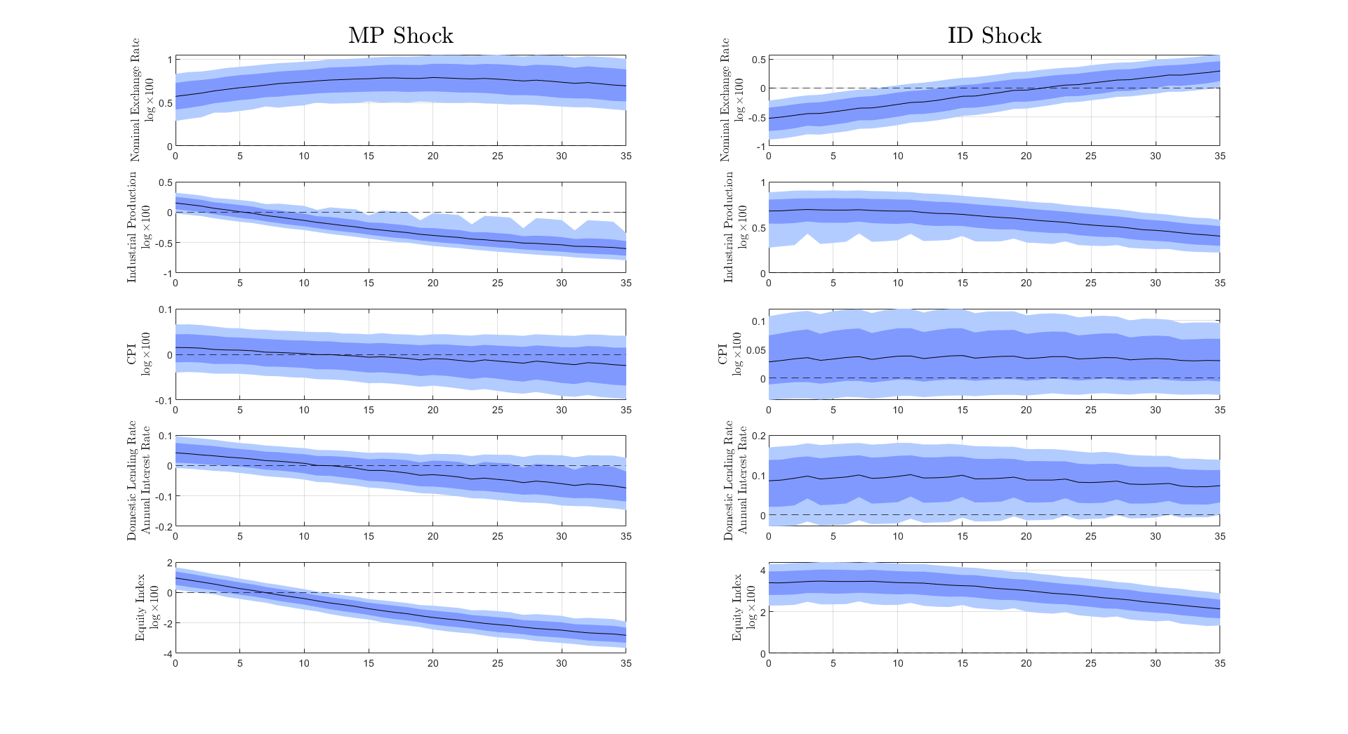
Figure 17: Impulse Response to One-Standard-Deviation Shock
Uniform Prior over Rotations

Note: The black solid line represents the median impulse response function. The dark shaded area represents the 16 and 84 percentiles. The light shaded are represents the 5 and 95 percentiles. The figure is comprised of 10 sub-figures ordered in five rows and two columns. Every row represents a different variable: (i) the MP structural FOMC shock, (ii) the ID structural FOMC shock, (iii) nominal exchange rate, (iv) industrial production index, (v) consumer price index, (vi) lending rate, (vii) equity index. The first column presents the results for the MP or “Pure US Monetary Policy” shock, the middle column the ID or “Information Disclosure” shock and the the last column presents the results following the “Standard High Frequency” identification shock. In the text, when referring to Panel $(i,j)$, $i$ refers to the row and $j$ to the column of the figure.

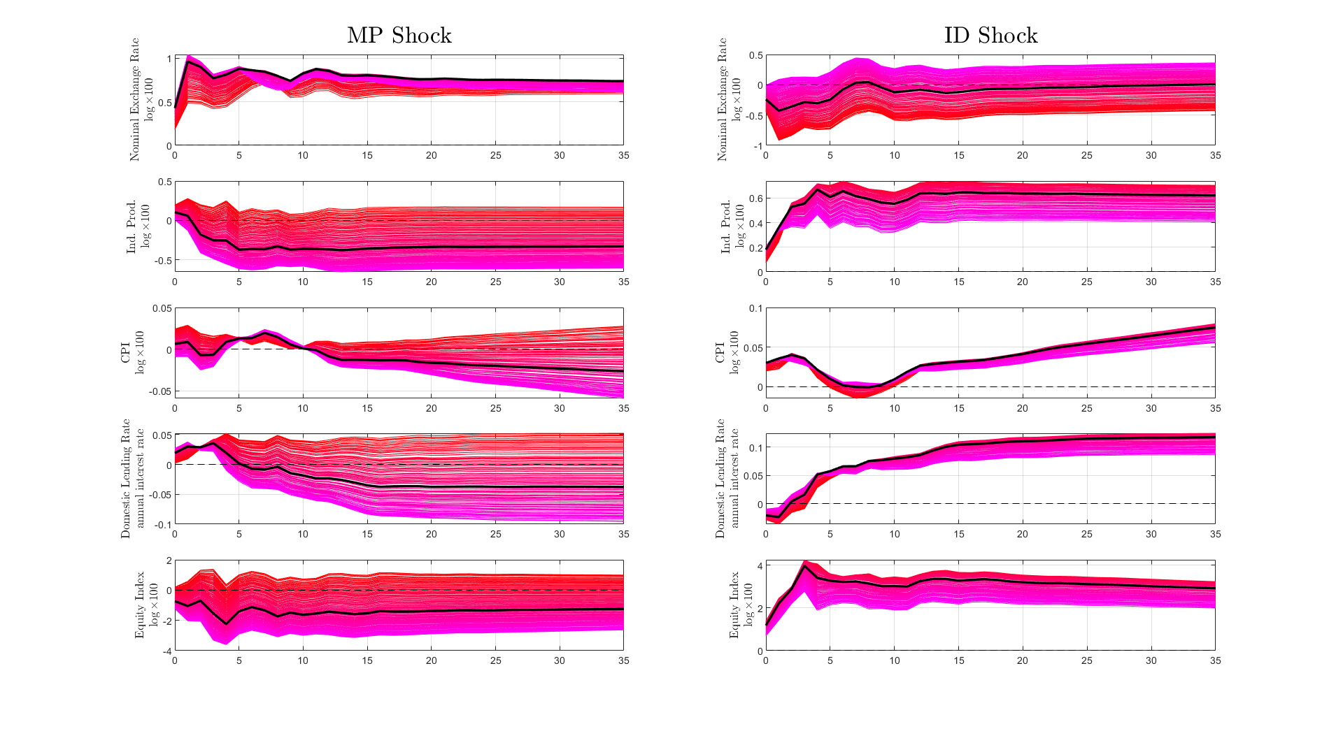
Figure 18: Impulse Response to One-Standard-Deviation Shock
Medians across Rotations

Note: Each line represents the median impulse response function of estimating the SVAR model using acceptable rotational angle $p$ where $p=0.01,\ldots,0.99$. The color of the lines varies from red (closer to 1) to purple (closer to 99). The solid black line represents the median impulse response using the median acceptable rotational angle. The figure is comprised of 10 sub-figures ordered in five rows and two columns. Every row represents a different variable: (i) the MP structural FOMC shock, (ii) the ID structural FOMC shock, (iii) nominal exchange rate, (iv) industrial production index, (v) consumer price index, (vi) lending rate, (vii) equity index. The first column presents the results for the MP or “Pure US Monetary Policy” shock, the second column the ID or “Information Disclosure” shock. In the text, when referring to Panel $(i,j)$, $i$ refers to the row and $j$ to the column of the figure.

Appendix D Alternative Strategies that Control for Information Effects

In this section, I show that the main results of this paper are also present when estimating the spillovers of a pure US monetary policy shock using alternative identification strategies which control for possible information effects around FOMC meetings. This result strengthens the argument that recent atypical international dynamics found when following the standard high-frequency identification strategy of US monetary policy shock, such as the expansion of industrial output, can be attributed to the systematic disclosure of information around FOMC meetings.

I consider two alternative identification strategies: the one proposed by Miranda-Agrippino and Ricco [2021] and the one presented by Bauer and Swanson [2022]. These two alternative identification strategies control for information effects of the Federal Reserve’s monetary policy through different approaches to that followed by Jarociński and Karadi [2020]. First, Miranda-Agrippino and Ricco [2021] define US monetary policy shocks as exogenous shifts in the policy instrument that surprise market participants, are unforecastable, and are not due to the central bank’s systematic response to its own assessment of the macroeconomic outlook. To this end, the authors construct an instrument constructed by regressing the high-frequency market surprises in the fourth federal fund future onto a set of Greenbook forecasts for output, inflation and unemployment. Through this instrument, the authors can control for the signalling effect of monetary policy, i.e., the Federal Reserve responding to expected changes in macroeconomic and financial variables. Unlike Jarociński and Karadi [2020], this approach controls for the Federal Reserve’s own information set which may or may not reflect or include the financial market’s information.

Second, Bauer and Swanson [2022] define US monetary policy shocks as exogenous shifts in policy interest rates that are purged of any response of the Federal Reserve to macroeconomic news. To do so, the authors identify US monetary policy shocks by orthogonalizing the high-frequency surprises of the first component of four Eurodollar futures contracts of key macroeconomic or financial information available prior to the FOMC meeting. The authors argue these approach purges the interest rate surprises of the ”Fed Response to News” channel, in which incoming, publicly available economic news causes both the Fed to change monetary policy and the private sector to revise its forecasts. It is noteworthy to state that this identification strategy is based on a previous paper, Bauer and Swanson [2020], which argues that the “Fed Information Effect”, as presented by Jarociński [2022], is not quantitatively important. Furthermore, the authors argue that a plausible explanation to this effect is the “Fed Response to News” channel. However, as stressed by Jarociński [2022] the theoretical models presented in Bauer and Swanson [2020, 2022] still predict a negative correlation between interest rate surprises and stock price surprises. Furthermore, even as the overall correlation between the high-frequency surprises between interest rates and the S&P 500 is negative, to the extent that some variants of the “Fed Response to News” channel generates a positive correlation between these financial surprises, one can interpret the ID shock as a proxy for this effect too (see Jarociński [2022]).

Figure 19 compares the impulse response functions using the two shocks constructed by Bauer and Swanson [2022]: (i) the un-cleansed or un-orthogonalized shock, (ii) the cleansed or orthogonalized shock.

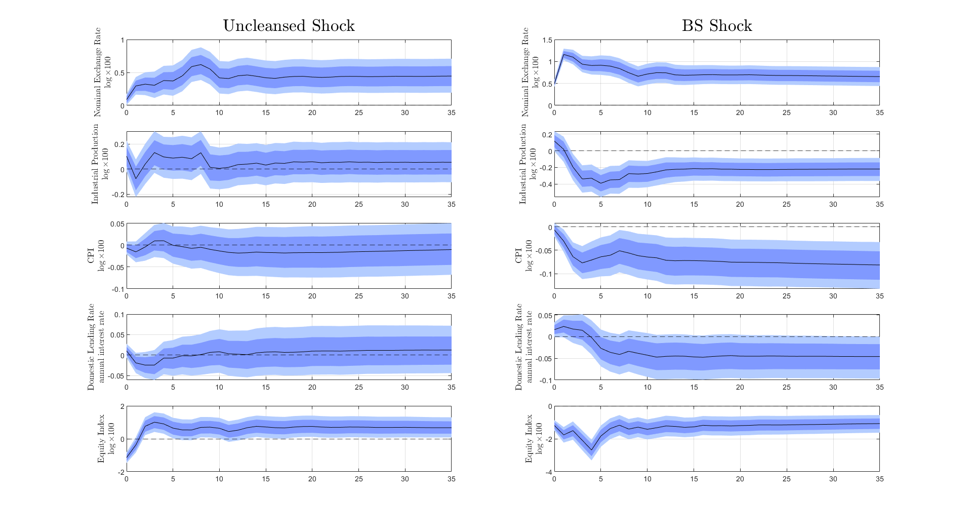
Figure 19: Impulse Response to Bauer and Swanson [2022] Shocks

Note: The black solid line represents the median impulse response function. The dark shaded area represents the 16 and 84 percentiles. The light shaded are represents the 5 and 95 percentiles. The figure is comprised of 10 sub-figures ordered in five rows and two columns. Every row represents a different variable: (i) nominal exchange rate, (ii) industrial production index, (iii) consumer price index, (iv) lending rate, (v) equity index. The first column presents the results for the un-cleansed or un-orthogonalized shock, the second column presents the results for the orthogonalized shock. In the text, when referring to Panel $(i,j)$, $i$ refers to the row and $j$ to the column of the figure.

On the left column, the un-orthogonalized shock leads to a atypical dynamics, such as a non-depreciation on impact of the exchange rate and a mild expansion of the industrial production and equity indexes. On the right column, the orthogonalized shocks lead to a significant depreciation on impact which is persistent across time, and a significant drop in both the industrial production and equity index. Thus, the un-cleansed shocks lead to dynamics similar to those arising from following the “Standard HFI” strategy used in Section 3. Additionally, using a monetary policy shock purged of information effects leads to results similar to those estimated for the MP shock in Section 3.

Figure 20 compares the impulse response functions of a MP shock under the benchmark specifications, with the impulse response functions of a US monetary policy shock under the two alternative identification strategies.

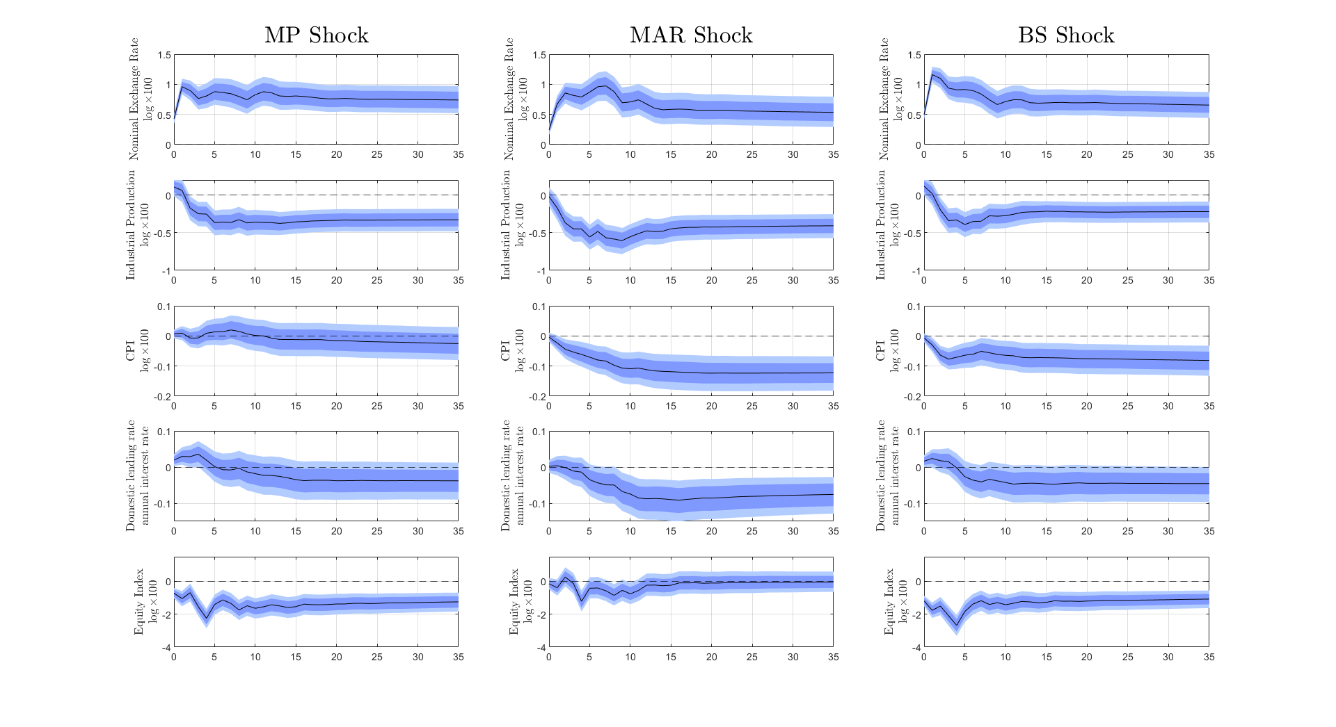
Figure 20: Impulse Response to One-Standard-Deviation Shock
Benchmark Specification

Note: The black solid line represents the median impulse response function. The dark shaded area represents the 16 and 84 percentiles. The light shaded are represents the 5 and 95 percentiles. The figure is comprised of 15 sub-figures ordered in five rows and three columns. Every row represents a different variable: (i) nominal exchange rate, (ii) industrial production index, (iii) consumer price index, (iv) lending rate, (v) equity index. The first column presents the results for the MP or “Pure US Monetary Policy” shock under the benchmark specification, the middle column presents the results for MAR shock or Miranda-Agrippino and Rey [2020], and the last column presents the results for the BS shock or Bauer and Swanson [2022]. In the text, when referring to Panel $(i,j)$, $i$ refers to the row and $j$ to the column of the figure.

The resulting impulse response functions are qualitatively in line with the main results presented in Section 3. All three specifications of a US monetary policy shock leads to a nominal exchange rate depreciation, a hump-shaped fall in industrial production, a drop in the consumer price index, a mild increase in lending rates and a persistent drop in the equity index. Quantitatively the results are also significantly close across the three identification strategies. While the two alternative identification strategies predict a greater and more significant reduction in the consumer price index, the benchmark specification predicts a greater increase in domestic lending rates and a larger and more persistent drop in the equity index. In summary, the robustness check in which two alternative identification strategies which control for the disclosure of information by the Federal Reserve around FOMC meetings lead to similar qualitatively and quantitatively results to our benchmark results leads to two main conclusions. First, by controlling for the disclosure of information around FOMC meetings, a pure US monetary policy shock leads to negative spillovers over a panel of countries, consistent with the older and conventional view. The second conclusion is that the systematic disclosure of information about the state of the US economy during FOMC announcements leads to recent atypical dynamics, such as those presented by Ilzetzki and Jin [2021] and the ones presented in Section 3 under the “Standard HFI” strategy. Once the ID shocks are taking into account, whether interpreted as the “Fed Information Effect” or the “Fed Response to News” channel, any atypical dynamics disappear.

Appendix E Potential Sources of Quantitative Heterogeneity

Following, I describe two potential sources of quantitatively heterogeneity in the international impact of US interest rates: (i) countries’ exchange rate regimes and (ii) countries’ reliance on the export of commodity goods. I briefly comment how previous literature has theorized that these country characteristics may influence the quantitative impact of the spillovers of US interest rates and describe my results.

Country classification for heterogeneity identification. Next, I describe the different classification/categorization of countries used in Section 4. In particular, I classified countries according to their exchange rate regimes and Emerging Market economies according to their commodity good dependence.

First, I classified/categorized countries according to their exchange rate regimes. In particular, I considered two partitions: (i) Peru vs the rest of the sample, (ii) Peru and Indonesia vs the rest of the sample. This sample partition is constructed following the exchange rate classification built by Ilzetzki et al. [2017] and additional evidence coming from both policy makers and other papers in the literature. All countries part of the Euro Zone are classified as freely floating. Hungary, Iceland and Sweden are classified as de facto narrow band with the Euro, de-coupling their currencies from the US dollar, given that the Euro is classified as freely floating.

Table 4: Exchange Rate Classification
Sourced from Ilzetzki et al. [2017]

Emerging Markets
Brazil	2003-2007: Freely Floating, 2008-2016: Managed Floating
Chile	2000-2007: De facto moving band that is narrower than or equal to +/-5%
	2008-2016: Managed Floating
Colombia	Managed Floating
Hungary	De facto crawling band +/- 2% since 2009. Euro. Broader band prior.
Indonesia	Starting 2005 De facto crawling band +/-2 to 5% range.
Mexico	2000-2008: De facto moving band that is narrower than or equal to +/-5%
	2009-2016 Managed Floating.
Peru	Starting from 2002. De facto crawling band +/-2%. US dollar
Philippines	Starting from 2002. De facto crawling band +/-2%. US dollar
South Africa	2000-2016 Freely floating
Advanced Economies
Australia	2000-2016: Freely floating
Canada	2003-Onward: Freely Floating
France	Freely Floating
Iceland	Manage floating
Italy	Freely Floating
Japan	2000-2016: Freely Floating
South Korea	2000-2003: De facto moving band that is narrower than or equal to +/-5%
	2004-2009 Managed Floating
	2010-2016: De facto moving band that is narrower than or equal to +/-5%
The Netherlands	Freely Floating
Sweden	De facto moving band +/-2% since 2008. Euro.

Table 4 presents the exchange rate classifications from Ilzetzki et al. [2017]. Evidence suggests that Peru has the tightest exchange rate regime (with a de facto moving band of less than 2%), with Indonesia being a close second (de facto moving band with periods below 2% and other periods below 5%). Additionally, as commented in Section 4, both the Central Banks of Peru and Indonesia, and the economic literature have highlighted or studied these countries as case studies of foreign exchange rate intervention policies, see Rossini et al. [2013, 2019], Castillo et al. [2021] for the case of Peru and Warjiyo [2013] for the case of Indonesia. While South Korea also presents a de facto narrow band the Central Bank of Korea publicly denies interventions. As commented by Ryoo et al. [2013], the Korean Central Bank does not carry out FX interventions directly and only does it sporadically through private banks. Consequently, in order to construct the sub-sample between countries which employ tight exchange rate regimes and the rest of the sample I only consider Peru and the “Peru & Indonesia” group.

Second, I carried out a sample partition exercise according to Emerging Market’s commodity dependence.

Table 5: Classification of Countries according to Commodity Dependence

Emerging Markets	Share of Commodity Goods in Total Exports		Classification
	2009-2010	2014-2015
Brazil	63	63	High Commodity Dependence
Chile	88	86	High Commodity Dependence
Colombia	76	81	High Commodity Dependence
Indonesia	62	58	Low Commodity Dependence
Mexico	25	19	Low Commodity Dependence
Peru	89	88	High Commodity Dependence
Philippines	15	19	Low Commodity Dependence
South Africa	54	55	Low Commodity Dependence

The first two columns of Table 5 presents data on the share of commodity goods in countries’ total export baskets as constructed by the UNCTAD’s “The State of Commodity Dependence” report. All countries in the sample export commodity goods, with Peru showing the greatest share of commodity goods in total exports (89% and 88% for the 2009-2010 and 2014-2015 periods), and Mexico showing the lowest share of commodity goods in total exports (25% and 19% for the 2009-2010 and 2014-2015 periods).

I classify the countries in the Emerging Market economies sample into “High Commodity Dependence” and “Low Commodity Dependence” according to whether they are on the top/bottom half of share of commodity goods in total exports. I follow this approach as I only seek to explore commodity goods as a potential source of heterogeneity. It is clear that there are other potential sample partitions. Additionally, there are other exercises to test commodity exports as potential sources of heterogeneity on the impact of spillovers of US interest rates. I leave these exercises for future research.

First, I study whether countries’ exchange rate regimes may influence the quantitative impact of the spillovers of US interest rates. The advantages and disadvantages of different exchange rate regimes is a classic yet still open question in international economics (see Mundell [1963], Levy-Yeyati and Sturzenegger [2003], Edwards and Yeyati [2005]). Moreover, the evidence is also mixed in terms of exchange rate regimes shaping the impact of US interest rates. On the one hand, Di Giovanni and Shambaugh [2008] provides evidence that for a panel of advanced economies the impact of higher foreign interest rates lead to a recession for countries with a fixed exchange rate. On the other hand, Rey [2015] argues that economies can not insulate from the US interest rate, even with flexible exchange rate regimes.

I carry two different partitions of the countries in the sample according to their exchange rate regimes. The first compares the resulting dynamics between a sample of only Peru versus the rest of the countries in the sample. The Peruvian Central Bank actively and publicly intervenes in foreign exchange rate markets to stabilize the nominal exchange rate. Also, the Peruvian case has been considered as a case study for the benefits and costs of FX interventions (see Rossini et al. [2019], Castillo et al. [2021] and Camara et al. [2021]). Figures 21 and 22 in Appendix C presents the impulse response functions to the MP and ID shocks for each sub-sample. On the one hand, across the two FOMC shocks, Peru exhibits a lower impact on the nominal exchange rate and on domestic lending rates as expected given its Central Bank interventions in foreign markets. The more moderate impact on the nominal exchange rate and domestic lending is particularly significant when comparing with a sample of Emerging Markets which excludes Peru (right-most column of Figures 21 and 22). On the other hand, the median response on industrial production are quantitatively close, while the impact on the equity index is significantly greater for Peru.

The second country partition groups Peru and Indonesia as countries with a “dirty float” exchange rate regime versus the rest of the countries in the sample. The grouping of Peru and Indonesia is motivated by both countries being classified as “tight” exchange rate managers according to Ilzetzki et al. [2017]. Figures 23 and 24 in Appendix C shows the impulse response functions of the MP and ID shock for each sub-sample, respectively. The insights of the first partition specification still hold.

Second, I study whether a country’s share of commodity goods in total exports matters for the transmission of US interest rate spillovers. In order to test the potential role of commodity goods as a source of heterogeneity in the spillovers of US interest rates I partition the sample of Emerging Market economies into “High Commodity Dependence” and “Low Commodity Dependence” countries. This partition is based on countries’ share of commodity goods in their export basket as constructed by the UNCTAD’s “The State of Commodity Dependence” for the year 2016. The high commodity dependence sample is comprised of Brazil, Chile, Colombia and Peru; while the low commodity dependence sample is comprised of Indonesia, Mexico, Philippines and South Africa. Hungary is dropped of the sample as it is not reported in the UNCTAD state of commodity dependence.

Figures 26 and 27 present the impulse response functions for the high and low commodity dependence samples respectively. I plot a dashed red line with the median response for the sample of Emerging Market economies (see Figure 25). In response to a MP shock, the low commodity dependence sample exhibits a greater nominal exchange rate depreciation, a greater pass through to consumer prices, a greater increase in EMBI spreads and a larger drop in the equity index, than the high commodity dependence sample. Similar dynamics arise in response to a ID shock. While this may be driven by large commodity exporters being having a greater tradable sector than other countries which reduces the economic contraction necessary to adjust to a given cut-off capital outflow, as suggested by Cavallo and Frankel [2008], I leave this question for future research.

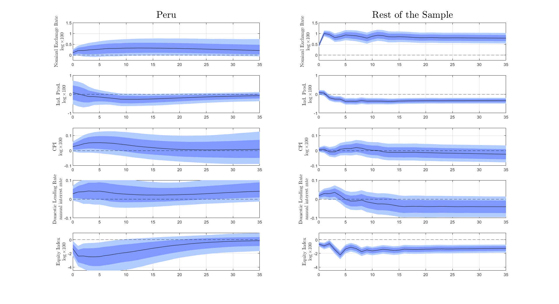
Figure 21: IRF to One-Standard-Deviation MP Shock
Exchange Rate Regimes - Peru

Note: The black solid line represents the median impulse response function. The dark shaded area represents the 16 and 84 percentiles. The light shaded are represents the 5 and 95 percentiles. The figure is comprised of 15 sub-figures ordered in five rows and three columns. Every row represents a different variable: (i) nominal exchange rate, (ii) industrial production index, (iii) consumer price index, (iv) lending rate, (v) equity index. The first column presents the results for Peru, the middle column presents the results for a sample of both Advanced and Emerging Market economies except Peru, the third or right column presents the results for a sample of Emerging Market economies except Peru. In the text, when referring to Panel $(i,j)$, $i$ refers to the row and $j$ to the column of the figure.

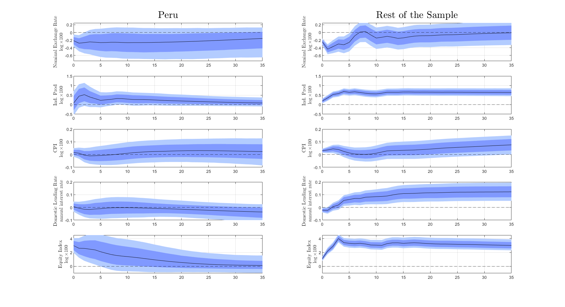
Figure 22: IRF to One-Standard-Deviation CBI Shock
Exchange Rate Regimes - Peru

Note: The black solid line represents the median impulse response function. The dark shaded area represents the 16 and 84 percentiles. The light shaded are represents the 5 and 95 percentiles. The figure is comprised of 15 sub-figures ordered in five rows and three columns. Every row represents a different variable: (i) nominal exchange rate, (ii) industrial production index, (iii) consumer price index, (iv) lending rate, (v) equity index. The first column presents the results for Peru, the middle column presents the results for a sample of both Advanced and Emerging Market economies except Peru, the third or right column presents the results for a sample of Emerging Market economies except Peru. In the text, when referring to Panel $(i,j)$, $i$ refers to the row and $j$ to the column of the figure.

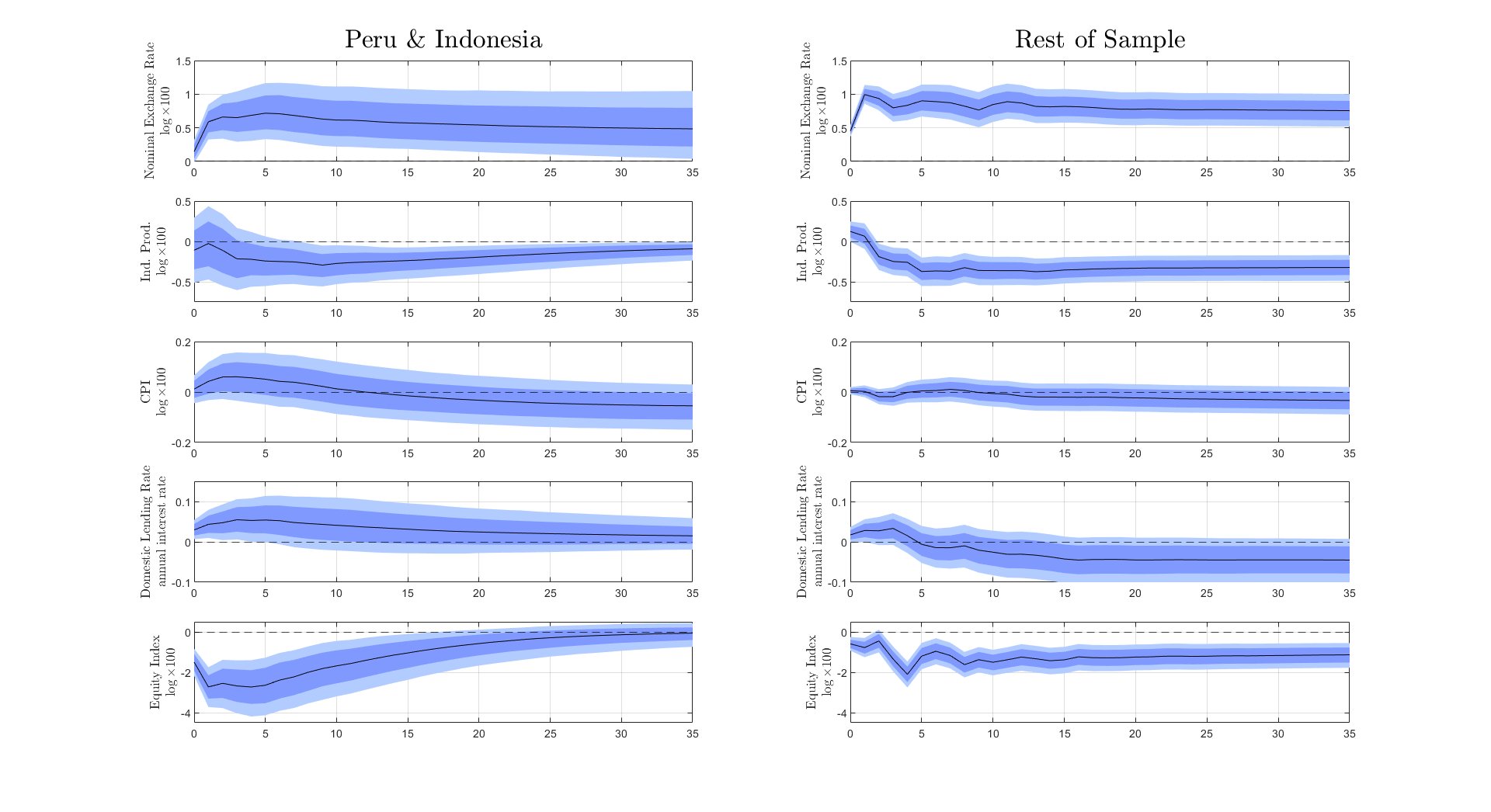
Figure 23: IRF to One-Standard-Deviation MP Shock
Exchange Rate Regimes - P & I

Note: The black solid line represents the median impulse response function. The dark shaded area represents the 16 and 84 percentiles. The light shaded are represents the 5 and 95 percentiles. The figure is comprised of 15 sub-figures ordered in five rows and three columns. Every row represents a different variable: (i) nominal exchange rate, (ii) industrial production index, (iii) consumer price index, (iv) lending rate, (v) equity index. The first column presents the results for a sample of Peru and Indonesia, the middle column presents the results for a sample of both Advanced and Emerging Market economies except Peru and Indonesia, the third or right column presents the results for a sample of Emerging Market economies except Peru and Indonesia. In the text, when referring to Panel $(i,j)$, $i$ refers to the row and $j$ to the column of the figure.

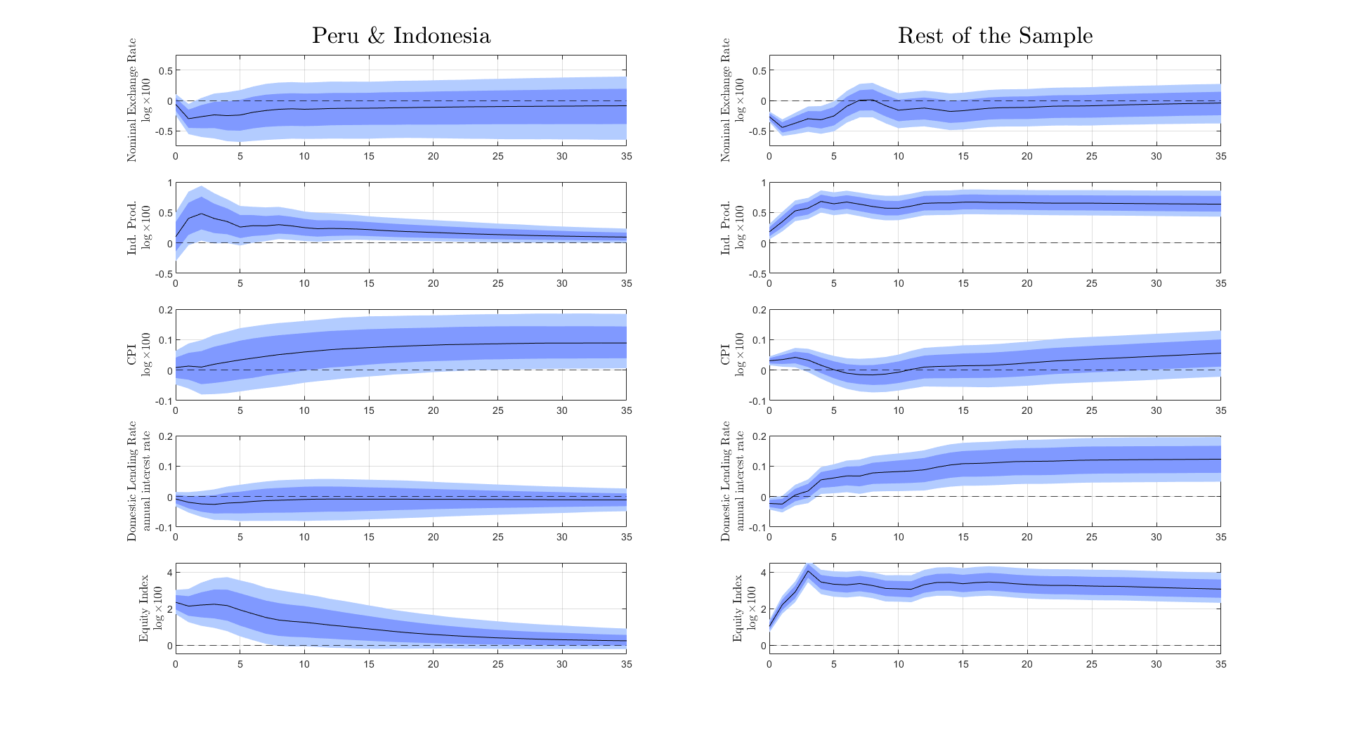
Figure 24: IRF to One-Standard-Deviation ID Shock
Exchange Rate Regimes - P & I

Note: The black solid line represents the median impulse response function. The dark shaded area represents the 16 and 84 percentiles. The light shaded are represents the 5 and 95 percentiles. The figure is comprised of 15 sub-figures ordered in five rows and three columns. Every row represents a different variable: (i) nominal exchange rate, (ii) industrial production index, (iii) consumer price index, (iv) lending rate, (v) equity index. The first column presents the results for a sample of Peru and Indonesia, the middle column presents the results for a sample of both Advanced and Emerging Market economies except Peru and Indonesia, the third or right column presents the results for a sample of Emerging Market economies except Peru and Indonesia. In the text, when referring to Panel $(i,j)$, $i$ refers to the row and $j$ to the column of the figure.

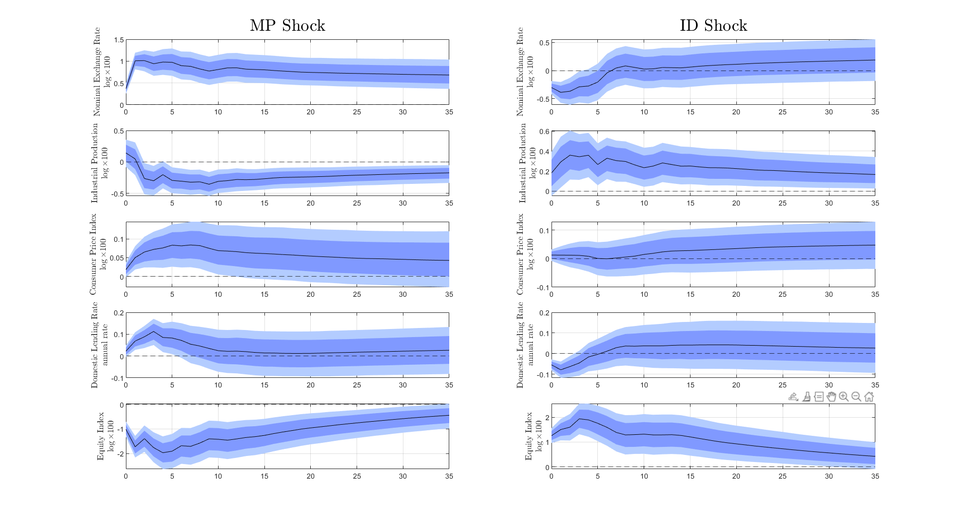
Figure 25: Impulse Response to One-Standard-Deviation Shock
EMs without Hungary

Note: The black solid line represents the median impulse response function. The dark shaded area represents the 16 and 84 percentiles. The light shaded are represents the 5 and 95 percentiles. The figure is comprised of 10 sub-figures ordered in five rows and two columns. Every row represents a different variable: (i) the MP structural FOMC shock, (ii) the ID structural FOMC shock, (iii) nominal exchange rate, (iv) industrial production index, (v) consumer price index, (vi) lending rate, (vii) equity index. The first column presents the results for the MP or “Pure US Monetary Policy” shock, the second column the ID or “Information Disclosure” shock. In the text, when referring to Panel $(i,j)$, $i$ refers to the row and $j$ to the column of the figure.

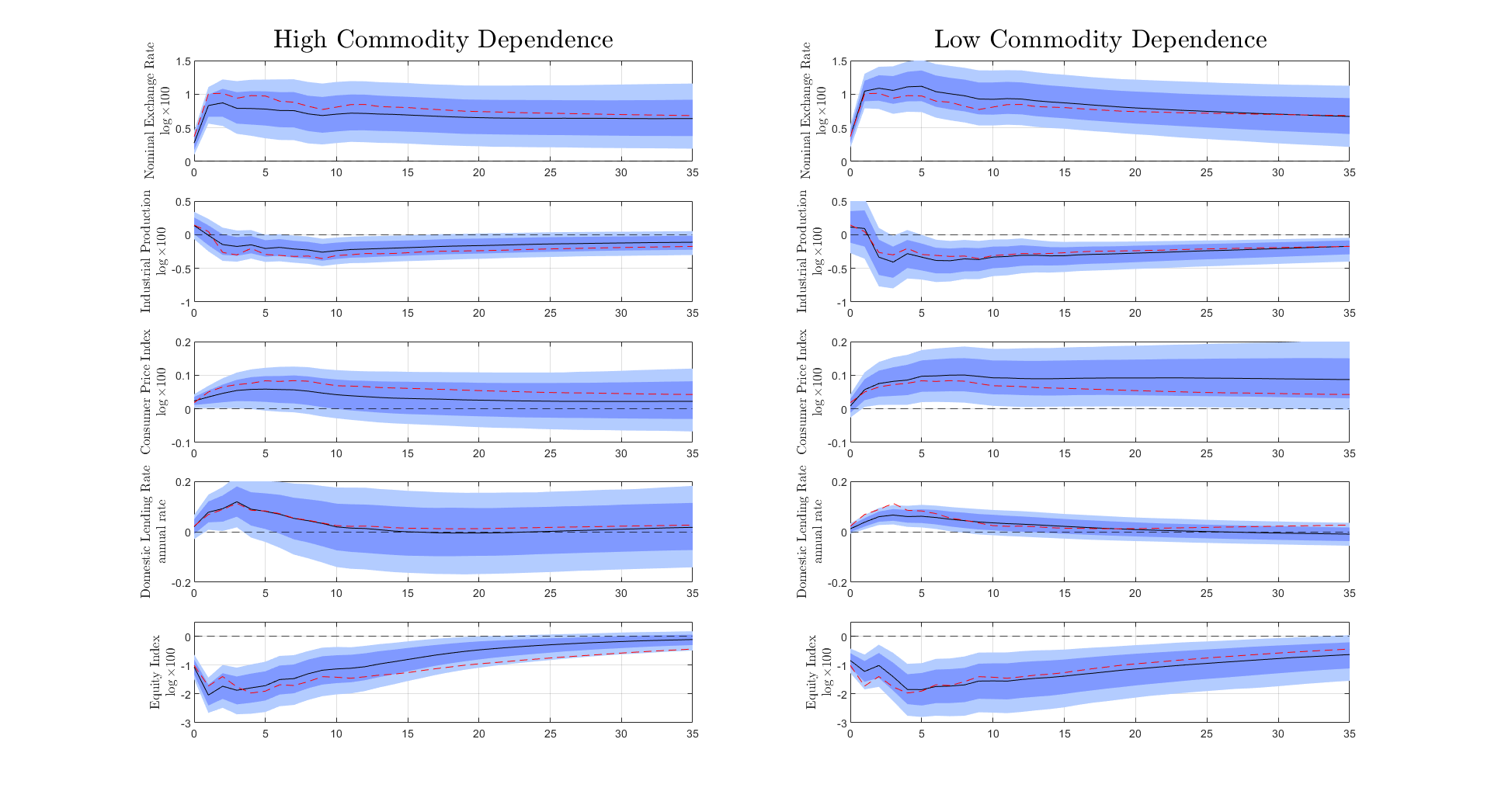
Figure 26: Impulse Response to One-Standard-Deviation MP Shock
Commodity Dependence

Note: The black solid line represents the median impulse response function. The dark shaded area represents the 16 and 84 percentiles. The light shaded are represents the 5 and 95 percentiles. The figure is comprised of 10 sub-figures ordered in five rows and two columns. Every row represents a different variable: (i) the MP structural FOMC shock, (ii) the ID structural FOMC shock, (iii) nominal exchange rate, (iv) industrial production index, (v) consumer price index, (vi) lending rate, (vii) equity index. The first column presents the results for the MP or “Pure US Monetary Policy” shock, the second column the ID or “Information Disclosure” shock. In the text, when referring to Panel $(i,j)$, $i$ refers to the row and $j$ to the column of the figure.

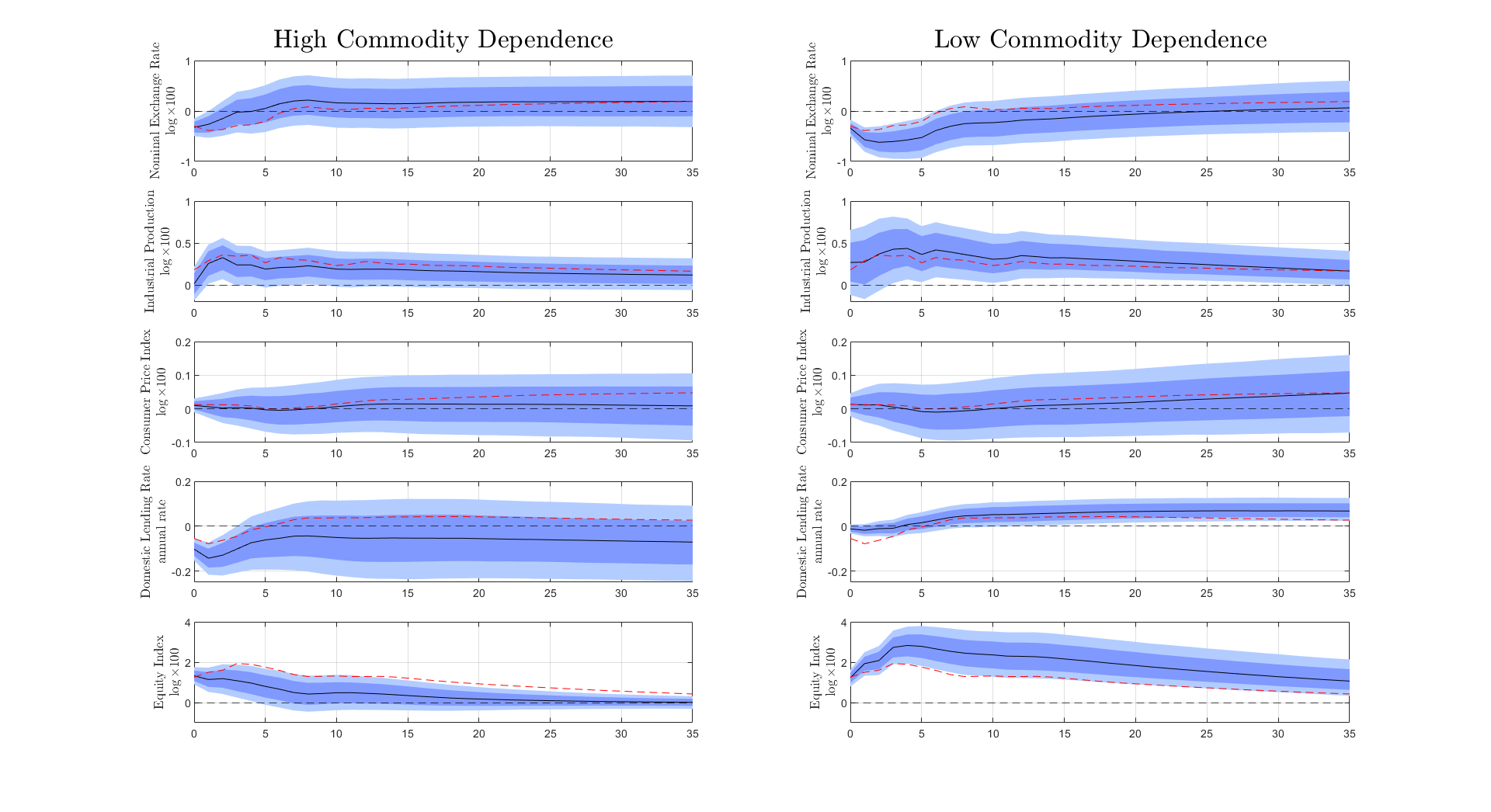
Figure 27: Impulse Response to One-Standard-Deviation ID Shock
Commodity Dependence

Note: The black solid line represents the median impulse response function. The dark shaded area represents the 16 and 84 percentiles. The light shaded are represents the 5 and 95 percentiles. The figure is comprised of 10 sub-figures ordered in five rows and two columns. Every row represents a different variable: (i) the MP structural FOMC shock, (ii) the ID structural FOMC shock, (iii) nominal exchange rate, (iv) industrial production index, (v) consumer price index, (vi) lending rate, (vii) equity index. The first column presents the results for the MP or “Pure US Monetary Policy” shock, the second column the ID or “Information Disclosure” shock. In the text, when referring to Panel $(i,j)$, $i$ refers to the row and $j$ to the column of the figure.

References

- Abraham et al. [2020] Facundo Abraham, Juan Jose Cortina Lorente, and Sergio L Schmukler. Growth of global corporate debt: Main facts and policy challenges. World Bank Policy Research Working Paper, 1(9394), 2020.
- Ahmed et al. [2021] Shaghil Ahmed, Ozge Akinci, and Albert Queralto. Us monetary policy spillovers to emerging markets: Both shocks and vulnerabilities matter. FRB of New York Staff Report, 1(972), 2021.
- Andrade and Ferroni [2021] Philippe Andrade and Filippo Ferroni. Delphic and odyssean monetary policy shocks: Evidence from the euro area. Journal of Monetary Economics, 117:816–832, 2021.
- Auclert et al. [2021] Adrien Auclert, Matthew Rognlie, Martin Souchier, and Ludwig Straub. Exchange rates and monetary policy with heterogeneous agents: Sizing up the real income channel. Technical report, National Bureau of Economic Research, 2021.
- Bauer and Swanson [2020] Michael D Bauer and Eric T Swanson. The fed’s response to economic news explains the” fed information effect”. Technical report, National Bureau of Economic Research, 2020.
- Bauer and Swanson [2022] Michael D Bauer and Eric T Swanson. A reassessment of monetary policy surprises and high-frequency identification. Technical report, National Bureau of Economic Research, 2022.
- Betts and Devereux [2000] Caroline Betts and Michael B Devereux. Exchange rate dynamics in a model of pricing-to-market. Journal of international Economics, 50(1):215–244, 2000.
- Broner et al. [2013] Fernando A Broner, Guido Lorenzoni, and Sergio L Schmukler. Why do emerging economies borrow short term? Journal of the European Economic Association, 11(suppl_1):67–100, 2013.
- Camara and Ramirez-Venegas [2022] Santiago Camara and Sebastian Ramirez-Venegas. The transmission of us monetary policy shocks: The role of investment & financial heterogeneity. Working Paper, 2022.
- Camara et al. [2021] Santiago Camara, Lawrence Christiano, and Husnu Dalgic. Sterilized fx interventions: Benefits and risks. Working Paper, 2021.
- Canova [2005] Fabio Canova. The transmission of us shocks to latin america. Journal of Applied econometrics, 20(2):229–251, 2005.
- Canova and Ciccarelli [2013] Fabio Canova and Matteo Ciccarelli. Panel Vector Autoregressive Models: A Survey. Emerald Group Publishing Limited, 2013.
- Castillo et al. [2021] Paul Castillo, Juan Pablo Medina, et al. Foreign exchange intervention, capital flows, and liability dollarization. Technical report, City University of Hong Kong, Department of Economics and Finance, Global …, 2021.
- Cavallo and Frankel [2008] Eduardo A Cavallo and Jeffrey A Frankel. Does openness to trade make countries more vulnerable to sudden stops, or less? using gravity to establish causality. Journal of International Money and Finance, 27(8):1430–1452, 2008.
- Cortina et al. [2018] Juan J Cortina, Tatiana Didier, and Sergio L Schmukler. Corporate debt maturity in developing countries: Sources of long and short-termism. The World Economy, 41(12):3288–3316, 2018.
- Dages et al. [2000] B Gerard Dages, Linda S Goldberg, and Daniel Kinney. Foreign and domestic bank participation in emerging markets: Lessons from mexico and argentina. Economic Policy Review, 6(3), 2000.
- Dedola et al. [2017] Luca Dedola, Giulia Rivolta, and Livio Stracca. If the fed sneezes, who catches a cold? Journal of International Economics, 108:S23–S41, 2017.
- Degasperi et al. [2020] Riccardo Degasperi, Seokki Hong, and Giovanni Ricco. The global transmission of us monetary policy. Working Paper, 2020.
- Di Giovanni and Shambaugh [2008] Julian Di Giovanni and Jay C Shambaugh. The impact of foreign interest rates on the economy: The role of the exchange rate regime. Journal of International economics, 74(2):341–361, 2008.
- Dieppe et al. [2016] Alistair Dieppe, Romain Legrand, and Björn Van Roye. The bear toolbox. European Central Bank, 2016.
- Dornbusch [1976] Rudiger Dornbusch. Expectations and exchange rate dynamics. Journal of political Economy, 84(6):1161–1176, 1976.
- Edwards and Yeyati [2005] Sebastian Edwards and Eduardo Levy Yeyati. Flexible exchange rates as shock absorbers. European economic review, 49(8):2079–2105, 2005.
- Eichenbaum and Evans [1995] Martin Eichenbaum and Charles L Evans. Some empirical evidence on the effects of shocks to monetary policy on exchange rates. The Quarterly Journal of Economics, 110(4):975–1009, 1995.
- Fleming [1962] J Marcus Fleming. Domestic financial policies under fixed and under floating exchange rates. Staff Papers, 9(3):369–380, 1962.
- Frenkel [1983] Jacob Frenkel. Monetary policy: Domestic targets and international constraints, 1983.
- García-Cicco and García-Schmidt [2020] Javier García-Cicco and Mariana García-Schmidt. Revisiting the exchange rate pass through: A general equilibrium perspective. Journal of International Economics, 127:103389, 2020.
- Gertler and Karadi [2015] Mark Gertler and Peter Karadi. Monetary policy surprises, credit costs, and economic activity. American Economic Journal: Macroeconomics, 7(1):44–76, 2015.
- Gürkaynak et al. [2004] Refet S Gürkaynak, Brian P Sack, and Eric T Swanson. Do actions speak louder than words? the response of asset prices to monetary policy actions and statements. The Response of Asset Prices to Monetary Policy Actions and Statements (November 2004), 2004.
- Ilzetzki and Jin [2021] Ethan Ilzetzki and Keyu Jin. The puzzling change in the international transmission of us macroeconomic policy shocks. Journal of International Economics, 130:103444, 2021.
- Ilzetzki et al. [2017] Ethan Ilzetzki, Carmen M Reinhart, and Kenneth S Rogoff. The country chronologies to exchange rate arrangements into the 21st century: will the anchor currency hold? Technical report, National Bureau of Economic Research, 2017.
- Jarocinski [2020] Marek Jarocinski. Central bank information effects and transatlantic spillovers. Working Paper, 2020.
- Jarociński [2022] Marek Jarociński. Central bank information effects and transatlantic spillovers. Journal of International Economics, page 103683, 2022.
- Jarociński and Karadi [2020] Marek Jarociński and Peter Karadi. Deconstructing monetary policy surprises—the role of information shocks. American Economic Journal: Macroeconomics, 12(2):1–43, 2020.
- Jordà [2005] Òscar Jordà. Estimation and inference of impulse responses by local projections. American economic review, 95(1):161–182, 2005.
- Levy-Yeyati and Sturzenegger [2003] Eduardo Levy-Yeyati and Federico Sturzenegger. To float or to fix: Evidence on the impact of exchange rate regimes on growth. American economic review, 93(4):1173–1193, 2003.
- Miranda-Agrippino and Rey [2020] Silvia Miranda-Agrippino and Hélene Rey. Us monetary policy and the global financial cycle. The Review of Economic Studies, 87(6):2754–2776, 2020.
- Miranda-Agrippino and Ricco [2021] Silvia Miranda-Agrippino and Giovanni Ricco. The transmission of monetary policy shocks. American Economic Journal: Macroeconomics, 13(3):74–107, 2021.
- Mundell [1963] Robert A Mundell. Capital mobility and stabilization policy under fixed and flexible exchange rates. Canadian Journal of Economics and Political Science/Revue canadienne de economiques et science politique, 29(4):475–485, 1963.
- Nakamura and Steinsson [2018] Emi Nakamura and Jón Steinsson. High-frequency identification of monetary non-neutrality: the information effect. The Quarterly Journal of Economics, 133(3):1283–1330, 2018.
- Obstfeld and Rogoff [1995] Maurice Obstfeld and Kenneth Rogoff. Exchange rate dynamics redux. Journal of political economy, 103(3):624–660, 1995.
- Pesaran and Smith [1995] M Hashem Pesaran and Ron Smith. Estimating long-run relationships from dynamic heterogeneous panels. Journal of econometrics, 68(1):79–113, 1995.
- Rey [2015] Hélène Rey. Dilemma not trilemma: the global financial cycle and monetary policy independence. Technical report, National Bureau of Economic Research, 2015.
- Rossini et al. [2013] Renzo Rossini, Zenon Quispe, and Enrique Serrano. Foreign exchange intervention in peru. BIS Paper, 1(73r), 2013.
- Rossini et al. [2019] Renzo Rossini, Adrian Armas, Paul Castillo, and Zenon Quispe. International reserves and forex intervention in peru. BIS Paper, 1(104q), 2019.
- Rubio-Ramirez et al. [2010] Juan F Rubio-Ramirez, Daniel F Waggoner, and Tao Zha. Structural vector autoregressions: Theory of identification and algorithms for inference. The Review of Economic Studies, 77(2):665–696, 2010.
- Ryoo et al. [2013] Sangdai Ryoo, Taeyong Kwon, and Hyejin Lee. Foreign exchange market developments and intervention in korea. BIS Paper, 1(73o), 2013.
- Stavrakeva and Tang [2019] Vania Stavrakeva and Jenny Tang. The dollar during the great recession: Us monetary policy signaling and the flight to safety. Working Paper, 2019.
- Svensson and Van Wijnbergen [1989] Lars EO Svensson and Sweder Van Wijnbergen. Excess capacity, monopolistic competition, and international transmission of monetary disturbances. The Economic Journal, pages 785–805, 1989.
- Uribe and Yue [2006] Martin Uribe and Vivian Z Yue. Country spreads and emerging countries: Who drives whom? Journal of international Economics, 69(1):6–36, 2006.
- Vicondoa [2019] Alejandro Vicondoa. Monetary news in the united states and business cycles in emerging economies. Journal of International Economics, 117:79–90, 2019.
- Warjiyo [2013] Perry Warjiyo. Indonesia: stabilizing the exchange rate along its fundamental. BIS Paper, 1(73m), 2013.