Pattern-Division Multiplexing for Multi-User Continuous-Aperture MIMO

Abstract

In recent years, thanks to the advances in meta-materials, the concept of continuous-aperture MIMO (CAP-MIMO) is reinvestigated to achieve improved communication performance with limited antenna apertures. Unlike the classical MIMO composed of discrete antennas, CAP-MIMO has a quasi-continuous antenna surface, which is expected to generate any current distribution (i.e., pattern) and induce controllable spatial electromagnetic (EM) waves. In this way, the information is directly modulated on the EM waves, which makes it promising to approach the ultimate capacity of finite apertures. The pattern design is the key factor to determine the communication performance of CAP-MIMO, but it has not been well studied in the literature. In this paper, we develop pattern-division multiplexing (PDM) to design the patterns for CAP-MIMO. Specifically, we first study and model a typical multi-user CAP-MIMO system, which allows us to formulate the sum-rate maximization problem. Then, we develop a general PDM technique to transform the design of the continuous pattern functions to the design of their projection lengths on finite orthogonal bases, which can overcome the challenge of functional programming. Utilizing PDM, we further propose a block coordinate descent (BCD) based pattern design scheme to solve the formulated sum-rate maximization problem. Simulation results show that, the sum-rate achieved by the proposed scheme is higher than that achieved by benchmark schemes, which demonstrates the effectiveness of the developed PDM for CAP-MIMO.

I Introduction

From 3G to 5G, the system performance of wireless communications has been greatly improved by the wide use of multiple-input multiple-output (MIMO) [2, 3, 4]. Equipped with multiple discrete antennas with half-wavelength spacing, MIMO is capable of enhancing the wireless transmissions by exploiting spatial multiplexing and diversity [5, 6, 7]. Inspired by the potential benefits of MIMO with an increasing number of antennas, exploring the ultimate transmission performance of a limited MIMO aperture has attracted extensive attention in the communication community. As an ultimate MIMO structure with extremely dense antennas, the concept of continuous-aperture MIMO (CAP-MIMO), which is also called as holographic MIMO [8, 9, 10, 11, 12], large intelligent surface (LIS) [13, 14, 15, 16], or reconfigurable intelligent surface (RIS) [17, 18, 19], is reinvestigated for wireless communications in recent years.

Figure 1: An example of CAP-MIMO based communication scenario.

Unlike the classical MIMO composed of multiple discrete antennas with half-wavelength spacing [2, 3, 4], by deploying a large number of sub-wavelength elements in a compact space, CAP-MIMO takes the form of a quasi-continuous electromagnetic (EM) surface [17]. Thanks to the recent advances of highly-flexible reconfigurable antennas, some early attempts at reconfigurable quasi-continuous apertures have been made [20, 21, 22, 23]. For example, the authors in [24] proposed a design method for synthesizing the binary meta-hologram pattern implemented in a leaky waveguide that can radiate signals towards a prescribed direction. Besides, by densely deploying a large number of small metamaterial elements based on electrical resonators, the research in [25] reported a continuous-aperture metasurface to achieve high array gain with limited size. In addition, the authors in [26] realized a electric-driven metasurface, and the EM wave with arbitrary polarization can be generated and radiated.

As shown in Fig. 1, an ideal CAP-MIMO is expected to have full control freedom of generating any current distribution on its spatially-continuous surface [10], so that its radiated EM waves can be artificially configured in a desired manner. In this way, the information for receivers can be directly modulated on the spatial EM waves and radiated to the physical space. Relying on this mechanism, the physical properties of spatial EM waves can be sufficiently exploited [27], leading to extreme spatial resolution [13, Fig. 5], high spectrum efficiency [14, Fig. 7] [15, Fig. 4] and high energy efficiency [17, Fig. 4]. Thus, CAP-MIMO becomes a promising technology to satisfy many challenging requirements of future wireless networks, such as the wide in-building coverage, high-speed uplink transmission, and high-accuracy localization [17].

I-A Prior Works

Realizing an ideal CAP-MIMO has a long history in the research field of micro-wave and photonics, dating back to Harold Wheeler’s work in 1965 [28] and David Staiman’s work in 1968 [29], respectively. By deriving the eigenfunctions of continuous-space EM channels, the capacity bound between two continuous volumes was derived in [30, 31]. The recent works on CAP-MIMO include antenna design [25], physical model [32], performance analysis [11], channel estimation [8], and so on. For example, the authors in [28] proposed to realize CAP-MIMO by exploiting the current sheet made of tightly coupled dipole array and the monolayer metallic made of magnetic particles. Then, to characterize the propagation process of the EM waves, the authors in [32] modeled the wireless channels between CAP-MIMO transceivers as Gaussian random fields. Subsequently, the author in [13] derived the analytical expressions of the spatial degrees of freedom (DoFs) of CAP-MIMO, and the authors in [11] further analyzed its near-field DoFs. Moreover, the authors in [8] proposed to exploit the geometrical property of arrays to realize the overhead-reduced channel estimation for CAP-MIMO. By utilizing special beam structures, a CAP-MIMO channel estimation scheme was proposed in [9], whose training overhead and complexity do not scale with the number of elements.

The pattern, i.e., the current distribution on the continuous aperture of CAP-MIMO, is the key factor determining the CAP-MIMO performance [13]. To support the coherent transmission of multiple data streams, it is necessary for CAP-MIMO transmitter to adopt a series of distinguishable patterns to carry different symbols [11, 12]. Specifically, the authors in [11] considered a near-field line-of-sight scenario, where one linear-aperture CAP-MIMO transmitter serves one linear-aperture EM-wave receiver. By adopting a series of square-wave functions to generate the patterns, the EM waves carrying different symbols can be radiated towards different spatial angles. Furthermore, the authors in [12] considered a similar near-field line-of-sight scenario with a couple of linear-aperture CAP-MIMO transceivers. Particularly, a wavenumber-division multiplexing (WDM) scheme was proposed to directly generate the patterns by Fourier basis functions. In this way, the transmitted symbols belonging to different streams are modulated on different spatial wavenumbers of radiated EM waves and transmitted, which is similar to the frequency-division multiplexing in conventional communications.

From the above discussions, we can find that, most existing works have directly adopted the patterns generated by given special functions to realize coherent transmission for CAP-MIMO [11, 12]. Although these schemes can improve the performance of CAP-MIMO to some extent, they only work efficiently in some special communication scenarios, such as single-user, linear-aperture, and/or near-field transmissions. To support CAP-MIMO in general scenarios with complex propagation environment and multiple distributed receivers, it is essential to design the patterns flexibly according to the continuous channel functions, which resembles the space-division multiplexing in conventional MIMO systems. Unfortunately, to the best of our knowledge, such a flexible and general pattern design scheme has not been well studied in the literature. One possible reason may be the mathematical challenge introduced by the design of continuous pattern functions of CAP-MIMO, which is usually non-convex functional programming [33] and thus difficult to be solved by the classical discrete signal processing techniques for conventional MIMO systems.

I-B Our Contributions

To fill in this gap, in this paper, we develop a general pattern-division multiplexing (PDM) technique to flexibly design patterns for multi-user CAP-MIMO. Our contributions are summarized as follows.

• Based on the EM propagation principle, we study and model a typical multi-user CAP-MIMO based communication system, where one CAP-MIMO transmitter with planar aperture serves multiple users coherently. This allows us to formulate the sum-rate maximization problem to optimize the CAP-MIMO patterns, and it also provides a possible framework for other technical problems in multi-user CAP-MIMO systems, such as channel estimation and energy efficiency optimization.

• We develop a general PDM technique to flexibly design the patterns of CAP-MIMO according to the knowledge of continuous channel functions. The key idea is to use series expansion to project the continuous pattern functions of CAP-MIMO onto an orthogonal basis space, thus the design of continuous pattern functions is transformed to the design of their projection lengths on finite orthogonal bases. In this way, the challenging problem of optimizing continuous patterns of CAP-MIMO can be addressed.

• Utilizing the developed PDM technique, we further propose a block coordinate descent (BCD) based pattern design scheme to solve the formulated sum-rate maximization problem for multi-user CAP-MIMO. Simulation results show that, the multi-user patterns designed by the proposed scheme are almost mutually orthogonal, and the sum-rate achieved by the proposed scheme is higher than that achieved by benchmark schemes.

I-C Organization and Notation

Organization: The rest of this paper is organized as follows. Section II introduces the system model of multi-user CAP-MIMO and formulates the problem of sum-rate maximization. The general PDM technique to address the continuous patterns of CAP-MIMO is developed in Section III, and the specific pattern design scheme to solve the formulated problem is proposed in Section IV. Simulation results are presented in Section V to validate the effectiveness of the proposed scheme. Finally, conclusions are drawn and future works are discussed in Section VI.

Notation: $\mathbb{C}$, $\mathbb{R}$, $\mathbb{R}_{+}$, and $\mathbb{Z}$ denote the set of complex, real, positive real, and integer numbers, respectively; ${[\cdot]^{-1}}$, ${[\cdot]^{*}}$, ${[\cdot]^{\rm T}}$, and ${[\cdot]^{\rm H}}$ denote the inverse, conjugate, transpose, and conjugate-transpose operations, respectively; $\|\cdot\|$ denotes the Euclidean norm of its argument; $\|\cdot\|_{\rm F}$ denotes the Frobenius norm of its argument; ${\rm det}\!\left|\,\cdot\,\right|$ denotes the determinant of its argument; $\mathbb{E}_{\bf z}\{\cdot\}$ is the expectation operator with respect to the random vector $\bf z$; $\mathfrak{R}\{\cdot\}$ denotes the real part of its argument; $\ln(\cdot)$ denotes natural logarithm; ${\rm rect}\left(\cdot\right)$ is the generalized rectangular function whose value takes one/zero when the condition in its argument is true/false; ${\rm mod}(a,b)$ denotes the remainder of $a/b$; $\nabla_{\mathbf{z}}$ denotes the first-order partial derivative operator with respect to $\bf z$; surfaces are indicated with calligraphic letters ${\cal S}$ and $\left|{{\cal S}}\right|$ denotes the Lebesgue measure of ${\cal S}$; $\mathbf{I}_{L}$ denotes an $L\times L$ identity matrix.

II System Model and Problem Formulation for CAP-MIMO

In this section, we study and model a typical multi-user CAP-MIMO based communication system, where one CAP-MIMO transmitter with planer aperture simultaneously serves $K$ users in the downlink. Specifically, we first introduce the system model of a CAP-MIMO transmitter in Subsection II-A. Then, the EM channels between the transmitter and the users are illustrated in Subsection II-B. Next, the EM waves at the users are modeled in Subsection II-C. Finally, the problem of the sum-rate maximization for multi-user CAP-MIMO system is formulated in Subsection II-D.

II-A CAP-MIMO Transmitter

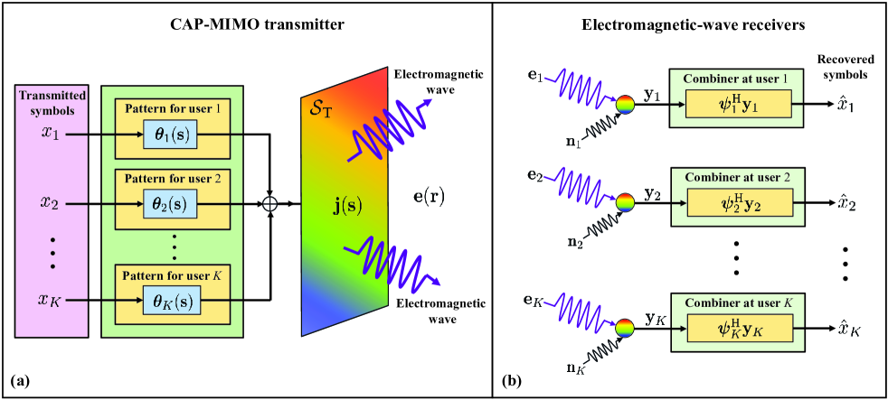
Figure 2: The concept of CAP-MIMO based wireless communications. (a) illustrates a CAP-MIMO transmitter, which has a quasi-continuous antenna aperture ${\cal S}_{\rm T}$ for radiating information-carrying EM waves ${\bf e}({\bf r})$. (b) illustrates $K$ tri-polarization single-antenna receivers (i.e., $K$ users) each being able to sense the three polarizations of incident wave ${\bf e}_{k}$ and then combine the three components via ${\bm{\psi}}_{k}$ to decode symbol $x_{k}$.

As shown in Fig. 2 (a), we consider a CAP-MIMO transmitter with aperture ${\cal S}_{\rm T}$ of area $A_{\rm T}=\left|{\cal S}_{\rm T}\right|$ working in a 3-D homogeneous medium. In the ideal case, CAP-MIMO has an almost continuous antenna aperture, which is able to generate any current distribution on its continuous surface for wireless communications [10, 11, 12, 13]. Let ${\bf j}({\bf s},t)\in{\mathbb{R}}^{3}$ denote the monochromatic current density at a generic location ${\bf s}:=\left(s_{x},s_{y},s_{z}\right)\in{\mathbb{R}}^{3}$ and time $t$. The ideally controllable current distribution at the CAP-MIMO transmitter can be written as

$$\mathbf{j}(\mathbf{s},t)=\Re\left\{\mathbf{j}(\mathbf{s})e^{-\mathrm{j}2\pi ft}\right\},~{}~{}{\mathbf{s}\in{{\cal S}_{\rm T}}},$$ (1)

where $f$ is the current frequency. For simplicity but without loss of generality, we assume that the communication system works in narrowband, which is exactly the well-known and widely-used time-harmonic assumption in EM analysis [34]. This allows us to ignore the time-related component $e^{-\mathrm{j}2\pi ft}$ and focus on the time-independent current density ${\bf j}({\bf s})\in{\mathbb{C}}^{3}$.

Consider that the CAP-MIMO transmitter simultaneously serves $K$ tri-polarization receivers (i.e., $K$ users) in the downlink. Let ${{\bf{x}}}\triangleq{\left[{{x_{1}},\cdots,{x_{K}}}\right]^{\rm T}}\in{{\mathbb{C}}^{K}}$ denote the symbols transmitted to $K$ users, respectively. We assume that these symbols have the normalized power, i.e., $\mathbb{E}_{\bf x}\left\{\mathbf{x}\mathbf{x}^{\rm H}\right\}=\mathbf{I}_{K}$. Then, similar to the conventional MIMO beamforming [35], the symbols $\bf x$ to be transmitted are modulated on $K$ different CAP-MIMO patterns $\left\{{{{\bm{\theta}}_{k}}\left({\bf{s}}\right)}\right\}_{k=1}^{K}$, which aims to make these symbols orthogonal at different users as much as possible, and thus high channel capacity can be achieved. For simplicity, we assume that CAP-MIMO employs linear superposition to combine multiple information-carrying patterns $\left\{{{{\bm{\theta}}_{k}}\left({\bf{s}}\right)}\right\}_{k=1}^{K}$ for coherent transmission, thus the combined current distribution ${\bf{j}}({\bf{s}})$ on the CAP-MIMO aperture can be modeled as

$${\bf{j}}({\bf{s}})=\sum\limits_{k=1}^{K}{{{\bm{\theta}}_{k}}\left({\bf{s}}\right){x_{k}}},~{}~{}{\mathbf{s}\in{{\cal S}_{\rm T}}},$$ (2)

where pattern ${\bm{\theta}}_{k}\left({\bf{s}}\right)\in{\mathbb{C}}^{3}$ is the component of current density that carries symbol $x_{k}$.

II-B Electromagnetic Channels

To model the radiated information-carrying EM waves in space, we define ${\bf e}({\bf r})\in\mathbb{C}^{3}$ as the electric field at point ${\bf r}:=\left(r_{x},r_{y},r_{z}\right)\in\mathbb{R}^{3}$, which is induced by the current distribution ${\bf j}({\bf s})$ on the CAP-MIMO aperture. According to Maxwell’s equations, the current distribution ${\bf j}({\bf r^{\prime}})$ and the electric field ${\bf e}({\bf r^{\prime}})$ satisfy the following inhomogeneous Helmholtz wave equation [34]:

$$\nabla\times\nabla\times\mathbf{e}\left(\mathbf{r}^{\prime}\right)-\kappa_{0}^{2}\mathbf{e}\left(\mathbf{r}^{\prime}\right)=\mathrm{j}\kappa_{0}Z_{0}\mathbf{j}\left(\mathbf{r}^{\prime}\right),$$ (3)

where ${\bf r^{\prime}}\in{\mathbb{R}}^{3}$ is any arbitrary point in space; $\kappa_{0}$ is the spatial wavenumber; and $Z_{0}$ is the intrinsic impedance of spatial medium, which is $376.73$ $\Omega$ in free space.

Then, to explicitly express the relationship between the current distribution ${\bf j}({\bf s})$ at the transmitter and the electric field ${\bf e}({\bf r})$ at the receiver, Green’s method [34] is utilized to solve (3). By introducing channel function $\mathbf{G}(\mathbf{r},\mathbf{s})\in{\mathbb{C}}^{3\times 3}$, the electric field ${\bf e}({\bf r})$ at point ${\bf r}$ can be induced from (3) as

$$\mathbf{e}(\mathbf{r})=\int_{{\cal S}_{\rm T}}\mathbf{G}(\mathbf{r},\mathbf{s})\mathbf{j}(\mathbf{s})\mathrm{d}\mathbf{s},$$ (4)

where channel function $\mathbf{G}(\mathbf{r},\mathbf{s})$ plays a role similar to the channel matrix in classical MIMO systems. From the perspective of mathematics, $\mathbf{G}(\mathbf{r},\mathbf{s})$ is the system impulse response, i.e., Green function. In particular, $\mathbf{G}(\mathbf{r},\mathbf{s})$ is determined by the specific wireless environment. For example, in ideal unbounded and homogeneous mediums, $\mathbf{G}(\mathbf{r},\mathbf{s})$ is [34]

$$\mathbf{G}(\mathbf{r},\mathbf{s})=\frac{\mathrm{j}\kappa_{0}Z_{0}}{4\pi}\frac{e^{\mathrm{j}\kappa_{0}\|\mathbf{r}-\mathbf{s}\|}}{\|\mathbf{r}-\mathbf{s}\|}\left(\mathbf{I}_{3}-\frac{(\mathbf{r}-\mathbf{s})(\mathbf{r}-\mathbf{s})^{\rm T}}{\|\mathbf{r}-\mathbf{s}\|^{2}}\right)$$ (5)

in the far field, while $\mathbf{G}(\mathbf{r},\mathbf{s})$ is usually modeled as a stochastic process in scattering environments [14].

II-C Electromagnetic-Wave Receivers

As shown in Fig. 2 (b), we assume that all $K$ EM-wave receivers (i.e., $K$ users) are located in the far-field region, and each user is equipped with an ideal tri-polarization antenna with area $A_{\rm R}=\frac{\lambda^{2}}{4\pi}$, which satisfies $A_{\rm R}\ll A_{\rm T}$ [15]. In this case, similar to a discrete antenna, each user can be reasonably approximated by a point in 3-D space.

Let ${\bf r}_{k}\in{\mathbb{R}}^{3}$ denote the 3-D location of the $k$-th user. In the ideal case, user $k$ with a tri-polarization antenna can sense the three polarizations of the EM waves reaching point ${\bf r}_{k}$ (i.e., holographic capability [11]). Then, the three polarization components are combined to decode symbol $x_{k}$ with a polarization combiner ${\bm{\psi}}_{k}\in{\mathbb{C}}^{3}$. Thus, according to (2) and (4), the EM wave received by user $k$ can be expressed as

$${{\bf{y}}_{k}}={{\bf{e}}_{k}}+{{\bf{n}}_{k}}= \underbrace{{x_{k}}\int_{{{\cal S}_{\rm{T}}}}{{{\bf{G}}_{k}}({\bf{s}})}{\bm{\theta}_{k}}\left({\bf{s}}\right){\rm{d}}{\bf{s}}}_{\text{Desired signal to user $k$}}+$$ (6)

$$\underbrace{\sum\limits_{j=1,j\neq k}^{K}{{x_{j}}\int_{{{\cal S}_{\rm{T}}}}{{{\bf{G}}_{k}}({\bf{s}}){\bm{\theta}_{j}}\left({\bf{s}}\right)}{\rm{d}}{\bf{s}}}}_{\text{Interferences from other users}}+\underbrace{{{\bf{n}}_{k}}}_{\text{Noise}},$$

where ${{\bf{e}}_{k}}:=\mathbf{e}(\mathbf{r}_{k})$, ${{\bf{G}}_{k}}({\bf s}):=\mathbf{G}(\mathbf{r}_{k},\mathbf{s})$, and ${{\bf{n}}_{k}}\in{\mathbb{C}}^{3}$ is the EM noise at user $k$, which is produced by all incoming EM waves that are not generated by the transmitter [34]. For simplicity, we follow the isotropic propagation assumption used in [12], thus ${{\bf{n}}_{k}}$ for all $k\in\{1,\cdots,K\}$ can be modeled as mutually independent additive white Gaussian noises with zero mean and variance $\sigma^{2}{\bf I}_{3}$. Our work can be easily extended to the general colored-noise case by replacing $\sigma^{2}{\bf I}_{3}$ in the following analysis with the specified $\mathbb{E}\left\{{\bf n}_{k}\mathbf{n}_{k}^{\mathrm{H}}\right\}$.

II-D Sum-Rate Maximization Problem Formulation

Based on the above system model, in this subsection, we formulate the sum-rate maximization problem for multi-user CAP-MIMO. By calculating the sum of multi-user mutual information, the sum-rate of $K$ users, can be derived from (6) as

$${R_{\rm sum}}=\sum\limits_{k=1}^{K}{{\log_{2}}\det\left|{{{\bf{I}}_{3}}+{{\bm{\alpha}}_{k}}{\bm{\alpha}}_{k}^{\rm{H}}{\bf{J}}_{k}^{-1}}\right|},$$ (7)

where ${\bm{\alpha}}_{k}$ and ${\bf{J}}_{k}$ are respectively given by

$${{\bm{\alpha}}_{k}}\!=\! \int_{{{\cal S}_{\rm{T}}}}{{{\bf{G}}_{k}}({\bf{s}}){{\bm{\theta}}_{k}}\left({\bf{s}}\right){\rm d}{\bf{s}}},$$ (8)

$${{\bf{J}}_{k}}\!= \!\!\!\sum\limits_{j=1,j\neq k}^{K}\!\!{{\int_{{\cal S}_{\rm{T}}}\!\!\!{{{\bf{G}}_{k}}({\bf{s}}){{\bm{\theta}}_{j}}\left({\bf{s}}\right){\rm d}{\bf{s}}}}{{\left({\int_{{\cal S}_{\rm{T}}}\!\!\!{{{\bf{G}}_{k}}({\bf{s^{\prime}}}){{\bm{\theta}}_{j}}\left({\bf{s^{\prime}}}\right){\rm d}{\bf{s^{\prime}}}}}\right)}^{\!\!\!\rm{H}}}}\!\!\!+{\sigma^{2}}{{\bf{I}}_{3}}.$$

In practical systems, we are interested in investigating the maximum sum-rate subject to a given power constraint. By integrating the radial component of the Poynting vector over a sphere with infinite-length radius [34], we introduce the following lemma to upper-bound the total transmit power of CAP-MIMO in the sense of expectation.

Lemma 1 (Transmit power constraint of multi-user CAP-MIMO)

The total transmit power of the multi-user CAP-MIMO based communication systems can be upper-bounded by the following inequality:

$$\sum\limits_{k=1}^{K}{\int_{{{\cal S}_{\rm{T}}}}{{{\left\|{{{\bm{\theta}}_{k}}\left({\bf{s}}\right)}\right\|}^{2}}{\rm{d}}{\bf{s}}}}\leq{P_{\rm{T}}},$$ (9)

where $P_{\rm T}$ can be viewed as the allowable maximum “transmit power” of CAP-MIMO, which is implicitly associated with the physical radiation power and measured in ${\rm A}^{2}$ (or ${\rm mA}^{2}$).

Proof:

Please see Appendix A. ∎

By combing (7) and (9), the original problem of sum-rate maximization subject to the transmit power constraint can be formulated as

$$\!\!\!\!{\cal P}_{o}:~{}~{} \mathop{\max}\limits_{{{\bm{\theta}}}\left({\bf s}\right)}~{}~{}{R_{\rm sum}}=\sum\limits_{k=1}^{K}{{\log_{2}}\det\left|{{{\bf{I}}_{3}}+{{\bm{\alpha}}_{k}}{\bm{\alpha}}_{k}^{\rm{H}}{\bf{J}}_{k}^{-1}}\right|},$$ (10a)

$$~{}~{}{\rm s.t.}~{}~{}\sum\limits_{k=1}^{K}{\int_{{{\cal S}_{\rm{T}}}}{{{\left\|{{{\bm{\theta}}_{k}}\left({\bf{s}}\right)}\right\|}^{2}}{\rm{d}}{\bf{s}}}}\leq{P_{\rm{T}}},$$ (10b)

where ${\bm{\theta}}({\bf s})$ is defined as ${\bm{\theta}}({\bf s}):=\left\{{{{\bm{\theta}}_{k}}\left({\bf{s}}\right)}\right\}_{k=1}^{K}$. Our goal is to maximize the sum-rate in (10a) by appropriately designing the continuous pattern functions ${\bm{\theta}}({\bf s})$, i.e., the current distribution on the continuous aperture ${\cal S}_{\rm T}$ of CAP-MIMO.

Remark 1

Generally, the pattern design problems such as ${\cal P}_{o}$ in (10) are difficult to solve. The reason is that, the continuous pattern functions ${\bm{\theta}}({\bf s})$ within integrals exist in both optimization objective and constraint in problem ${\cal P}_{o}$ in (10), which is actually non-convex functional programming [33]. In this case, since the partial derivatives of the optimization objective with respect to ${\bm{\theta}}({\bf s})$ are difficult to obtain, the classical signal processing techniques for discrete arrays, such as gradient descent and Lagrange dual method [37], are hard to be adopted. Such kind of non-convex functional programming is common in the optics and micro-wave areas, especially for the design of the radiation patterns of directional antennas, and these problems are usually addressed by using commercial EM simulation software such as high frequency structure simulator (HFSS), which results in high time and space complexity.

III Developed Pattern-Division Multiplexing (PDM) for CAP-MIMO

To address the challenging optimization of continuous pattern functions as shown in problem ${\cal P}_{o}$ in (10), in this section, we develop PDM technique to design CAP-MIMO patterns. The key idea is to use series expansion to expand the continuous pattern functions in an orthogonal basis space. In this way, the continuous pattern functions are projected onto finite orthogonal bases, thus the design of these functions is transformed to the design of their projection lengths in the orthogonal basis space, which makes optimizing continuous functions feasible. Specifically, in Subsection III-A, we introduce the developed PDM technique to deal with CAP-MIMO patterns. Then, in Subsection III-B, we provide the performance analysis of the developed PDM.

III-A A General Pattern-Division Multiplexing (PDM) Technique

Different from the existing methods which adopt the patterns directly generated by special functions for coherent transmissions [11, 12], in this section, we develop PDM technique to flexibly design the patterns for CAP-MIMO according to the knowledge of continuous channel functions $\left\{{{{\bf{G}}_{k}}}({\bf{s}})\right\}_{k=1}^{K}$. Particularly, the developed PDM aims to strengthen the desired information-carrying signals and make the EM waves carrying different symbols as much orthogonal as possible at the users. In this way, higher channel capacity is expected, which is similar to the space-division multiplexing in classical MIMO systems.

To efficiently optimize the continuous pattern functions $\left\{{{{\bm{\theta}}_{k}}({\bf{s}})}\right\}_{k=1}^{K}$ in problem ${\cal P}_{o}$ in (10), inspired by the pattern design methods in antenna theory, an intuitive idea is to use series expansion to project these continuous functions onto an orthogonal space [34]. In this paper, we use Fourier bases to expand the spatial continuous pattern functions. Since the Fourier transform of spatial domain is exactly the wavenumber domain, this choice of bases allows us to better understand and analyze the pattern design from the perspective of wavenumber space. In this way, we obtain the following lemma.

Lemma 2 (Fourier series expansion of pattern functions)

For an arbitrary continuous pattern function ${\bm{\theta}}_{k}({\bf s})\in{\mathbb{C}}^{3}$ defined in volume ${\bf s}:=\left(s_{x},s_{y},s_{z}\right)\in{\cal S}_{\rm T}$, if ${\bm{\theta}}_{k}({\bf s})$ is absolutely integrable, pattern function ${\bm{\theta}}_{k}({\bf s})$ to be designed can be equivalently rewritten as

$${\bm{\theta}}_{k}({\bf s})=\sum\limits_{\bf{n}}^{\infty}{{{\bf{w}}_{k,{\bf{n}}}}{\Psi_{\bf{n}}}\left({\bf{s}}\right)},~{}~{}{\bf s}\in{\cal S}_{\rm T},$$ (11)

where we define ${\bf{n}}:={\left({n_{x}},{n_{y}},{n_{z}}\right)}\in\mathbb{Z}^{3}$ and $\sum\nolimits_{\bf{n}}^{\infty}{}:=\sum\nolimits_{{n_{x}}=-\infty}^{\infty}{\sum\nolimits_{{n_{y}}=-\infty}^{\infty}{\sum\nolimits_{{n_{z}}=-\infty}^{\infty}{}}}$ to simplify notations. Particularly, the projection length ${{\bf{w}}_{k,{\bf{n}}}}\in{\mathbb{C}}^{3}$ in the wavenumber domain and the Fourier base function ${{\Psi_{\bf n}}\left({\bf s}\right)}\in{\mathbb{C}}$ can be written as

$${{\bf{w}}_{k,{\bf{n}}}}= \frac{1}{\sqrt{A_{\rm T}}}\int_{{\bf{s}}\in{\cal S}_{\rm T}}{{\bm{\theta}}_{k}({\bf s}){\Psi^{*}_{\bf{n}}}\left({\bf{s}}\right){\rm d}{\bf{s}}},~{}~{}{\bf{n}}\in\mathbb{Z}^{3},$$ (12a)

$${\Psi_{\bf{n}}}\left({\bf{s}}\right)= \frac{1}{\sqrt{A_{\rm T}}}{e^{2\pi{\rm j}\left({\frac{{{n_{x}}}}{{{L_{x}}}}\left(s_{x}-\frac{L_{x}}{2}\right)+\frac{{{n_{y}}}}{{{L_{y}}}}{\left(s_{y}-\frac{L_{y}}{2}\right)}+\frac{{{n_{z}}}}{{{L_{z}}}}{\left(s_{z}-\frac{L_{z}}{2}\right)}}\right)}},$$

$$~{}~{}{\bf s}\in{\cal S}_{\rm T},$$ (12b)

where $L_{x}$, $L_{y}$, and $L_{z}$ denote the maximum projection lengths of volume ${\cal S}_{\rm T}$ on the $x$-, $y$-, and $z$-axis of 3-D coordinate system, respectively. The Fourier bases ${\Psi_{\bf{n}}}\left({\bf{s}}\right)$ satisfy

$$\int_{{\bf{s}}\in{{\cal S}_{\rm T}}}{{\Psi_{\bf{n}}}\left({\bf{s}}\right)\Psi_{\bf{n}^{\prime}}^{*}\left({\bf{s}}\right)}{\rm{d}}{\bf{s}}=\left\{\begin{array}[]{l}1,~{}~{}{\bf n}^{\prime}={\bf n},\\ 0,~{}~{}{\bf n}^{\prime}\neq{\bf n},\end{array}\right.$$ (15)

which guarantees the orthogonality between any two basis functions.

Note that, different from the Fourier basis functions in [14] which represent the spatial plane-wave channels, the basis functions in (12) have no physical significance, which only provide functional degrees of freedom for the further optimization of pattern functions ${\bm{\theta}}({\bf s})$. Since their indexes ${\bf{n}}:={\left({n_{x}},{n_{y}},{n_{z}}\right)}\in\mathbb{Z}^{3}$ only take integer values, the equality $\left({2\pi n_{x}}/{L_{x}}\right)^{2}+\left({2\pi n_{y}}/{L_{y}}\right)^{2}+\left({2\pi n_{z}}/{L_{z}}\right)^{2}=\kappa_{0}^{2}$ does not hold in most cases. Then, using the series expansion in Lemma 2, the continuous pattern functions $\left\{{{{\bm{\theta}}_{k}}({\bf{s}})}\right\}_{k=1}^{K}$ in problem ${\cal P}_{o}$ in (10) can be equivalently replaced by their discrete projection lengths $\left\{{{{\bf{w}}_{k,{\bf{n}}}}}\right\}_{k=1}^{K}$ in the wavenumber space.

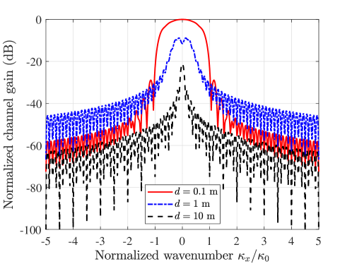
(a) $f=2.4$ GHz.

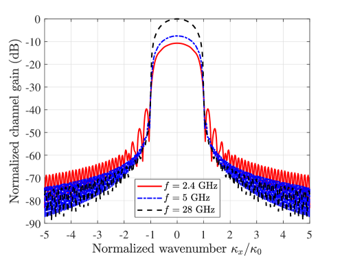
(b) $d=0.1$ m.

Figure 3: The normalized channel gain $\left\|{{\mathscr{F}}\left\{{{{\bf{G}}_{1}}({\bf{s}})}{\rm rect}\left({\bf s}\in{\cal S}_{\rm T}\right)\right\}}\right\|_{\rm{F}}^{2}$ against the normalized wavenumber $\kappa_{x}/\kappa_{0}$, where frequency is fixed as $f=2.4$ GHz in (a) and distance is fixed as $d=0.1$ m in (b).

To this end, we introduce the following two useful corollaries to address the continuous pattern functions:

Corollary 1 (Continuous-discrete transform for electric field)

Let ${\bm{\kappa}}:=\left({{\kappa_{x}},{\kappa_{y}},{\kappa_{z}}}\right)$ denote the wavenumber and ${\mathscr{F}}\left\{\cdot\right\}\left({{{\bm{\kappa}}}}\right)$ denote the Fourier transform of its argument on surface ${\cal S}_{\rm T}$ at wavenumber ${\bm{\kappa}}$. By adopting Fourier series expansion for pattern function ${\bm{\theta}}_{j}({\bf{s}})$, the product of channel function ${\bf{G}}_{k}({\bf{s}})$ and pattern function ${\bm{\theta}}_{j}({\bf{s}})$ in integral $\int_{{{\cal S}_{\rm T}}}{\rm d}{\bf s}$ , i.e., the electric field, can be equivalently rewritten as

$$\int_{{{\cal S}_{\rm{T}}}} {{{\bf{G}}_{k}}({\bf{s}}){{\bm{\theta}}_{j}}\left({\bf{s}}\right){\rm d}{\bf{s}}}=\sum\limits_{\bf{n}}^{\infty}{{{\bf{\Omega}}_{k,{\bf{n}}}}{{\bf{w}}_{j,{\bf{n}}}}},$$ (16)

$$~{}~{}~{}~{}~{}\forall k,j\in\{1,\cdots,K\},$$

where

$${{\bf{\Omega}}_{k,{\bf{n}}}}={\mathscr{F}}\left\{{{{\bf{G}}_{k}}({\bf{s}})}\right\}\left({{{\bf{\bm{\kappa}}}_{\bf{n}}}}\right)=\int_{{{\cal S}_{\rm{T}}}}{{{\bf{G}}_{k}}({\bf{s}}){\Psi_{\bf{n}}}\left({\bf{s}}\right){\rm{d}}{\bf{s}}},$$ (17)

in which ${{{\bf{\Omega}}_{k,{\bf{n}}}}}\in{\mathbb{C}}^{3\times 3}$ is exactly the Fourier transform of function ${\bf{G}}_{k}({\bf s}){\rm rect}\left({\bf s}\in{\cal S}_{\rm T}\right)$ over the CAP-MIMO aperture ${\cal S}_{\rm T}$ at wavenumber ${\bm{\kappa}_{\bf{n}}}=(2\pi\frac{{n_{x}}}{L_{x}},2\pi\frac{{n_{y}}}{L_{y}},2\pi\frac{{n_{z}}}{L_{z}})$. In particular, according to Parseval’s theorem, the following equation naturally holds:

$$\int_{{{\cal S}_{\rm{T}}}}{\left\|{{{\bf{G}}_{k}}({\bf{s}})}\right\|_{\rm F}^{2}{\rm{d}}{\bf{s}}}=\sum\limits_{\bf{n}}^{\infty}{\left\|{{{\bf{\Omega}}_{k,{\bf{n}}}}}\right\|_{\rm F}^{2}},$$ (18)

where the left-hand side is the integral of the Frobenius norms of continuous functions while the right-hand side is the sum of the Frobenius norms of discrete matrices. Particularly, $\left\|{{{\bf{G}}_{k}}({\bf{s}})}\right\|_{\rm F}^{2}$ can be viewed as the channel gain in the spatial domain at position ${\bf r}_{k}$ and $\left\|{{{\bf{\Omega}}_{k,{\bf{n}}}}}\right\|_{\rm F}^{2}$ can be viewed as the channel gain in the wavenumber domain at wavenumber $\bm{\kappa}_{\bf{n}}$.

Corollary 2 (Continuous-discrete transform for power constraint)

According to Parseval’s theorem, the Euclidean norm of pattern function ${\bm{\theta}}_{k}\left({\bf{s}}\right)$ in integral $\int_{{{\cal S}_{\rm T}}}{\rm d}{\bf s}$, i.e., the transmit power of $x_{k}$, can be equivalently rewritten as

$$\int_{{{\cal S}_{\rm{T}}}}{{{\left\|{{{\bm{\theta}}_{k}}\left({\bf{s}}\right)}\right\|}^{2}}{\rm{d}}{\bf{s}}}=\sum\limits_{\bf{n}}^{\infty}{{{\left\|{{{\bf{w}}_{k,{\bf{n}}}}}\right\|}^{2}}},~{}~{}\forall k\in\{1,\cdots,K\},$$ (19)

which guarantees the conservation of system energy.

Utilizing the continuous-discrete transforms in Corollary 1 and Corollary 2, we note that the continuous functions $\left\{{{{\bf{G}}_{k}}}({\bf{s}})\right\}_{k=1}^{K}$ and $\left\{{{{\bm{\theta}}_{k}}({\bf{s}})}\right\}_{k=1}^{K}$ can be replaced by their projection lengths $\left\{{{{\bm{\Omega}}_{k,{\bf{n}}}}}\right\}_{k=1}^{K}$ and $\left\{{{{\bf{w}}_{k,{\bf{n}}}}}\right\}_{k=1}^{K}$, respectively. Thus, the functional programming [33] can be reformulated as a common digital signal processing problem. However, since the number of expansion items is infinite as shown in (16), (18) and (19), the optimization of projection lengths $\left\{{{{\bf{w}}_{k,{\bf{n}}}}}\right\}_{k=1}^{K}$ is still unacceptable for practical computing devices. Therefore, how to address the infinite expansion items becomes a critical issue for the pattern design of CAP-MIMO

Fortunately, thanks to the inherent physical properties of function ${\bf{G}}_{k}({\bf s}){\rm rect}\left({\bf s}\in{\cal S}_{\rm T}\right)$, some recent works have revealed that, the value of $\left\|{{{\bf{\Omega}}_{k,{\bf{n}}}}}\right\|_{\rm F}^{2}$, i.e., the channel gain in the wavenumber domain, is high in the low-wavenumber band and negligible in the high-wavenumber band in most cases. For example, the authors in [12] have shown by simulations that, in a typical system with two linear-aperture CAP-MIMO transceivers, the wavenumber-domain channel gain within the band of $[-\kappa_{0},\kappa_{0}]$ is usually much higher than that within the other bands [12, Fig. 4]. By deriving the closed-form expression of ${\mathscr{F}}\left\{{{{\bf{G}}}_{k}({\bf{s}})}{\rm rect}\left({\bf s}\in{\cal S}_{\rm T}\right)\right\}$, the authors in [38] have analytically proved that, the wavenumber-domain channel gain within the band of $[-\kappa_{0},\kappa_{0}]$ dominates in the whole wavenumber domain [38, Fig. 2, Fig. 3]. Some works on channel modeling have also pointed out that, the small-scale fading of CAP-MIMO channel can be modeled by the sum of finite Fourier plane-wave representations, which also implies that ignoring high-wavenumber expansion items has little impact on channel quality [10, Eq. (39)].

To observe the above fact, here we take a specific scenario for example. For simplicity, we consider a single-user CAP-MIMO system working at frequency $f$, where the CAP-MIMO transmitter is deployed on the x-axis with aperture ${{\cal S}_{\rm T}}=\left\{{{\left({{s_{x}},{s_{y}},{s_{z}}}\right)}{\Big{|}}\left|{{s_{x}}}\right|\leq 0.5\,{\rm{m}},{{s_{y}}}=0,{s_{z}}=0}\right\}$ and the user is located at $\left(0,0,d\right)$. Then, we plot the normalized channel gain $\left\|{{\mathscr{F}}\left\{{{{\bf{G}}_{1}}({\bf{s}})}{\rm rect}\left({\bf s}\in{\cal S}_{\rm T}\right)\right\}}\right\|_{\rm{F}}^{2}$ against the normalized wavenumber $\kappa_{x}/\kappa_{0}$ in Fig. 3 (a) and Fig. 3 (b) with different setups. From these two figures, one can observe that, for all our considered setups, the channel gain within the band of $\kappa_{x}\in[-\kappa_{0},\kappa_{0}]$ dominates in the wavenumber domain. Particularly, when $\left|\kappa_{x}/\kappa_{0}\right|$ is larger than 1, compared with $\left|\kappa_{x}/\kappa_{0}\right|=0$, the wavenumber-domain channel gain suffers a large loss of about -30 dB, which is in agreement with the results in existing works [12, 38, 10].

As a result, this fact inspires us to approximate the Fourier expansion series $\sum\nolimits_{\bf{n}}^{\infty}{{{\bf{\Omega}}_{k,{\bf{n}}}}{{\bf{w}}_{j,{\bf{n}}}}}$ with finite low-wavenumber and high-power items that satisfy $|2\pi\frac{{{n_{x}}}}{{{L_{x}}}}|\leq{\kappa_{0}}$, $|2\pi\frac{{{n_{y}}}}{{{L_{y}}}}|\leq{\kappa_{0}}$, and $|2\pi\frac{{{n_{z}}}}{{{L_{z}}}}|\leq{\kappa_{0}}$ and ignore those high-wavenumber and low-power items, which actually exploits the idea of compressed sensing [39]. In this way, we obtain the following proposition.

Proposition 1 (Finite-item approximation of expansion series)

Define ${\bf N}:=\left(N_{x},N_{y},N_{z}\right)$ with $N_{x}$, $N_{y}$, and $N_{z}$ being the numbers of the reserved expansion items on the x-, y-, and z-axis, respectively. Let $\sum\nolimits_{\bf{n}}^{\bf{N}}:=\sum\nolimits_{{n_{x}}=-{N_{x}}}^{{N_{x}}}{\sum\nolimits_{{n_{y}}=-{N_{y}}}^{{N_{y}}}{\sum\nolimits_{{n_{z}}=-{N_{z}}}^{{N_{z}}}{}}}$ for notation simplification. Then, the electric field in (16) and the transmit power in (19) can be approximated by

$$\!\!\!\!\!\!\int_{{{\cal S}_{\rm{T}}}}\!\!{{{\bf{G}}_{k}}({\bf{s}}){{\bm{\theta}}_{j}}\left({\bf{s}}\right){\rm d}{\bf{s}}} \!\approx\!\sum\limits_{\bf{n}}^{\bf N}{{{\bf{\Omega}}_{k,{\bf{n}}}}{{\bf{w}}_{j,{\bf{n}}}}},\forall k,j\in\{1,\cdots,K\},$$ (20a)

$$\int_{{{\cal S}_{\rm{T}}}}\!\!{{{\left\|{{{\bm{\theta}}_{k}}\left({\bf{s}}\right)}\right\|}^{2}}{\rm{d}}{\bf{s}}} \!\approx\!\sum\limits_{\bf{n}}^{\bf N}{{{\left\|{{{\bf{w}}_{k,{\bf{n}}}}}\right\|}^{2}}},~{}\forall k\in\{1,\cdots,K\},$$ (20b)

where the numbers of reserved expansion items ${\bf N}$ are suggested to be set to

$${N_{x}}=\left\lceil{\frac{{{\kappa_{0}}{L_{x}}}}{{2\pi}}}\right\rceil,~{}{N_{y}}=\left\lceil{\frac{{{\kappa_{0}}{L_{y}}}}{{2\pi}}}\right\rceil,~{}{N_{z}}=\left\lceil{\frac{{{\kappa_{0}}{L_{z}}}}{{2\pi}}}\right\rceil.$$ (21)

Proof:

Employ a truncation operation on (16) and (19), and then find the minimum positive integers $N_{x}$, $N_{y}$, and $N_{z}$ subject to $2\pi\frac{{{N_{x}}}}{{{L_{x}}}}\geq{\kappa_{0}}$, $2\pi\frac{{{N_{y}}}}{{{L_{y}}}}\geq{\kappa_{0}}$, and $2\pi\frac{{{N_{z}}}}{{{L_{z}}}}\geq{\kappa_{0}}$. ∎

Exploiting the above proposition, the total number of expansion items becomes finite, which is acceptable for the practical computing devices. For example, when $L_{x}=0.5$ m and $f=2.4$ GHz, the number of reserved items on the x-axis can be chosen as $N_{x}=\left\lceil{\frac{{{\kappa_{0}}{L_{x}}}}{2\pi}}\right\rceil=4$. In this way, it becomes feasible to design the continuous pattern functions $\left\{{{{\bm{\theta}}_{k}}({\bf{s}})}\right\}_{k=1}^{K}$ for CAP-MIMO via optimizing the finite projection lengths $\left\{{{{\bf{w}}_{k,{\bf{n}}}}}\right\}_{k=1}^{K}$ in the wavenumber space.

III-B Performance Analysis of Developed PDM Technique

Since the developed PDM includes a finite-item approximation as shown in Proposition 1, the CAP-MIMO system will suffer a performance loss. Nevertheless, it can be expected from Corollary 1 and Corollary 2 that, when the number of the reserved expansion items increases, this performance loss will approach zero asymptotically. In this subsection, to show the PDM’s capability of approaching the ideal solution asymptotically, we analyze the performance loss caused by the finite-item approximation. To this end, in order to make the problem analytically tractable and get insightful results, here we consider a simplified CAP-MIMO system with single user ($K=1$), while the general multi-user case will be studied in Section IV.

III-B1 Achievable user signal-to-noise ratio (SNR)

To analyze the performance loss caused by the finite-item approximation while employing PDM, we first study the achievable user SNR in the ideal case. Since $K=1$, for notation simplification, we temporarily omit the subscript $k$ of channel function ${{\bf{G}}_{k}}({\bf{s}})$, pattern function ${{\bm{\theta}}_{k}}\left({\bf{s}}\right)$, and polarization combiner $\bm{\psi}_{k}$, respectively. Then, the original sum-rate maximization problem ${\cal P}_{o}$ in (10) can be equivalently reformulated as the following SNR maximization problem:

$${\cal P}_{s}:~{}~{} \mathop{\max}\limits_{{\bm{\psi}},{{\bm{\theta}}}\left({\bf s}\right)}~{}~{}\gamma=\frac{{\left|{{{\bm{\psi}}^{\rm{H}}}\int_{{S_{\rm{T}}}}{\bf{G}}({\bf{s}}){\bm{\theta}}\left({\bf{s}}\right){\rm{d}}{\bf{s}}}\right|^{2}}}{{{{\bm{\psi}}^{\rm{H}}}{\bm{\psi}}{\sigma^{2}}}},$$ (22a)

$$~{}~{}{\rm s.t.}~{}~{}\int_{{{\cal S}_{\rm{T}}}}{{{\left\|{{\bm{\theta}}\left({\bf{s}}\right)}\right\|}^{2}}{\rm{d}}{\bf{s}}}\leq{P_{\rm{T}}},$$ (22b)

where $\gamma$ is the user SNR, and ${\bm{\psi}}\in{\mathbb{C}}^{3}$ is used to decode symbols at the user side, as shown in Fig. 2 (b).

Different from most CAP-MIMO systems whose performance limits are difficult to obtain due to the non-convex functional programming, we prove that the single-user CAP-MIMO system has a closed-form and optimal pattern design, given as below:

Lemma 3 (Achievable user SNR)

The maximum achievable SNR of the single-user CAP-MIMO system, i.e., the optimal solution to problem ${\cal P}_{s}$ in (22), can be expressed as

$${\gamma^{{\rm{opt}}}}=\frac{{{P_{\rm{T}}}}}{{{\sigma^{2}}}}{\lambda_{\max}}\left\{{\int_{{{\cal S}_{\rm{T}}}}{{{\bf{G}}}({\bf{s}}){\bf{G}}^{\rm{H}}({\bf{s}}){\rm{d}}{\bf{s}}}}\right\},$$ (23)

where $\lambda_{\max}\left\{\cdot\right\}$ denotes the maximum eigenvalue of its argument. In particular, the optimal user SNR ${\gamma^{{\rm{opt}}}}$ can be achieved when

$${\bm{\theta}}\left({\bf{s}}\right) \!=\!\frac{\sqrt{{P_{\rm{T}}}}{{{\bf{G}}^{\rm{H}}}({\bf{s}}){{\bm{\xi}}_{\max}}\left\{{\int_{{S_{\rm{T}}}}\!{{{\bf{G}}}({\bf{s}}^{\prime}){\bf{G}}^{\rm{H}}({\bf{s}}^{\prime}){\rm{d}}{\bf{s}}^{\prime}}}\right\}}}{{\sqrt{\int_{{{\cal S}_{\rm{T}}}}{{{\left\|{{{\bf{G}}^{\rm{H}}}({\bf{s}}){{\bm{\xi}}_{\max}}\left\{{\int_{{{\cal S}_{\rm{T}}}}\!{{{\bf{G}}}({\bf{s}}^{\prime}){\bf{G}}^{\rm{H}}({\bf{s}}^{\prime}){\rm{d}}{\bf{s}}^{\prime}}}\right\}}\right\|}^{2}}{\rm{d}}{\bf{s}}}}}},$$ (24a)

$${\bm{\psi}} \!=\!\frac{{{\bm{\xi}}_{\max}}\left\{{\int_{{{\cal S}_{\rm{T}}}}{{{\bf{G}}}({\bf{s}}){\bf{G}}^{\rm{H}}({\bf{s}}){\rm{d}}{\bf{s}}}}\right\}}{\left\|{{\bm{\xi}}_{\max}}\left\{{\int_{{{\cal S}_{\rm{T}}}}{{{\bf{G}}}({\bf{s}}){\bf{G}}^{\rm{H}}({\bf{s}}){\rm{d}}{\bf{s}}}}\right\}\right\|},$$ (24b)

where ${\bm{\xi}}_{\max}\left\{{\cdot}\right\}$ denotes the eigenvector corresponding to the maximum eigenvalue of its argument.

Proof:

Please see Appendix B. ∎

Remark 2

When the user is located in the far-field region, the squared channel function ${{\bf{G}}^{\rm{H}}}({\bf{s}}){\bf{G}}({\bf{s}})$ takes the similar amplitude for all ${\bf{s}}\in{\cal S}_{\rm T}$, thus we have ${\left\|{{{\bf{G}}^{\rm{H}}}({\bf{s}}){\bf{G}}({\bf{s}})}\right\|}\approx{\left\|{{{\bf{G}}^{\rm{H}}}({\bf{s}}_{0}){\bf{G}}({\bf{s}}_{0})}\right\|}$ wherein ${\bf{s}}_{0}$ is the central coordinate of ${\cal S}_{\rm T}$. In this case, it can be observed from (23) that, the achievable user SNR can be approximated by ${\gamma^{{\rm{opt}}}}\approx\frac{{{P_{\rm{T}}}}}{{{\sigma^{2}}}}{A_{\rm{T}}}\left\|{{{\bf{G}}^{\rm{H}}({\bf{s}}_{0})}{\bf{G}}({\bf{s}}_{0})}\right\|$, where $\left\|{{{\bf{G}}^{\rm{H}}({\bf{s}}_{0})}{\bf{G}}({\bf{s}}_{0})}\right\|$ can be viewed as the gain of channel between the CAP-MIMO transmitter and the user. One can find that, the achievable user SNR ${\gamma^{{\rm{opt}}}}$ is approximately proportional to the transmit SNR $\frac{{{P_{\rm{T}}}}}{{{\sigma^{2}}}}$ and the area of CAP-MIMO aperture $A_{\rm T}$.

III-B2 Performance loss caused by finite-item approximation

By combining Corollary 1 and Lemma 3, the achievable user SNR in the ideal case, i.e., $\gamma^{\rm opt}$ in (23), can be equivalently rewritten as

$${\gamma^{{\rm{opt}}}}=\frac{1}{{{\sigma^{2}}}}{\left\|{\sum\limits_{\bf{n}}^{\infty}{{{\bf{\Omega}}_{\bf{n}}}{{\bf{w}}_{\bf{n}}}}}\right\|^{2}},$$ (25)

where ${\bf{\Omega}}_{\bf{n}}$ and ${\bf{w}}_{\bf{n}}$ are the Fourier transform of ${\bf G}\left({\bf s}\right)$ on surface ${\cal S}_{\rm T}$ and the inverse Fourier transform of ${\bm{\theta}}\left({\bf s}\right)$ at wavenumber ${\bm{\kappa}}_{\bf n}$, respectively, written as

$${{\bf{\Omega}}_{\bf{n}}} =\int_{{{\cal S}_{\rm{T}}}}{{\bf{G}}\left({\bf{s}}\right){\Psi_{\bf{n}}}\left({\bf{s}}\right){\rm{d}}{\bf{s}}},$$ (26)

$${{\bf{w}}_{\bf{n}}} =\frac{1}{\sqrt{A_{\rm T}}}\int_{{{\cal S}_{\rm{T}}}}{{\bm{\theta}}\left({\bf{s}}\right)\Psi_{\bf{n}}^{*}\left({\bf{s}}\right){\rm{d}}{\bf{s}}}.$$ (27)

After employing the finite-item approximation in Proposition 1 for $\gamma^{\rm opt}$ in (25), the non-ideal achievable SNR ${\hat{\gamma}}$ can be written as:

$${\hat{\gamma}}=\frac{1}{{{\sigma^{2}}}}{\left\|{\sum\limits_{\bf{n}}^{\bf N}{{{\bf{\Omega}}_{\bf{n}}}{{\bf{w}}_{\bf{n}}}}}\right\|^{2}}.$$ (28)

To analytically evaluate the truncation error of the finite-item approximation in Proposition 1 on the system performance, here we define a new metric called SNR loss: $\Delta:={{{\gamma^{{\rm{opt}}}}-\hat{\gamma}}}$, which is related to the CAP-MIMO transmit power and the noise power at the user. Then, our goal is to derive the upper bound of the SNR loss $\Delta$ for a given $\bf N$, which characterizes the worst-case performance loss caused by the finite-item approximation in Proposition 1. By exploiting some inequality techniques, we obtain the following lemma:

Lemma 4 (Upper bound of SNR loss)

Given the numbers of the reserved Fourier expansion items ${\bf N}=\left(N_{x},N_{y},N_{z}\right)$, the SNR loss $\Delta$ can be upper-bounded by

$$\Delta\leq\frac{{{P_{\rm{T}}}}}{{{\sigma^{2}}}}\sqrt{1-\eta}\left({1+\sqrt{\eta}}\right)\int_{{{\cal S}_{\rm T}}}{\left\|{{\bf{G}}({\bf{s}})}\right\|_{\rm{F}}^{2}{\rm d}{\bf{s}}},$$ (29)

where $\eta\in[0,1]$ is defined as

$$\eta=\frac{{\sum\nolimits_{\bf{n}}^{\bf{N}}{\left\|{{{\bf{\Omega}}_{\bf{n}}}}\right\|_{\rm{F}}^{2}}}}{{\sum\nolimits_{\bf{n}}^{\infty}{\left\|{{{\bf{\Omega}}_{\bf{n}}}}\right\|_{\rm{F}}^{2}}}},$$ (30)

which can be regarded as a threshold describing the degree of finite-item approximation.

Proof:

Please see Appendix C. ∎

Remark 3

From (29) we can observe that, the upper bound of the SNR loss $\Delta$ is approximately proportional to the transmit SNR $\frac{{{P_{\rm{T}}}}}{{{\sigma^{2}}}}$ and the aperture area $A_{\rm T}$ of CAP-MIMO. It implies that, for a given $\bf N$, larger aperture area $A_{\rm T}$ will lead to larger performance loss. This explains why $\bf N$ should be set according to the aperture size, as shown in (21). Besides, when the number of the reserved expansion series $\bf N$ increases, i.e., $\eta\to 1$, the upper bound of the SNR loss $\Delta$ gradually goes to zero. It indicates that, despite the existence of the finite-item approximation, the performance loss can be artificially controlled by setting an acceptable $\bf N$ while employing the developed PDM. In this way, the pattern design scheme based on PDM is promising to approach the ideal solution asymptotically.

IV Proposed Pattern Design Scheme Based on PDM Technique

In this section, to show how to design CAP-MIMO patterns through the developed PDM technique, we propose a BCD based pattern design scheme to solve the sum-rate maximization problem ${\cal P}_{o}$ in (10) as a typical example. Specifically, in Subsection IV-A, we present the whole process of the scheme design. Then, in Subsection IV-B, the convergence and computational complexity of the proposed pattern design scheme are discussed.

IV-A Proposed Pattern Design Scheme for Sum-Rate Maximization

In this subsection, we propose a BCD based pattern design scheme to solve the sum-rate maximization problem ${\cal P}_{o}$ in (10). Firstly, we consider to decouple the continuous pattern functions by adopting an equivalent transform for sum-rate maximization problem [40, Theorem 1], and we obtain the following lemma.

Algorithm 1 Proposed pattern design scheme for the sum-rate maximization of multi-user CAP-MIMO systems.

0:     Channel functions ${{\bf{G}}_{k}\left({\bf s}\right)}$ with respect to ${\bf s}\in{\cal S}_{\rm T}$ for all users $k\in\{1,\cdots,K\}$.

0:     Optimized sum-rate $R_{{\rm sum}}$; optimized combiners $\bm{\psi}$ at users; optimized patterns $\bm{\theta}\left({\bf s}\right)$ on the aperture of CAP-MIMO transmitter.

1:  Initialize $\bm{\psi}$ and $\bm{\theta}\left({\bf s}\right)$;

2:  while No convergence of $R_{{\rm sum}}$ do

3:     Update ${\bm{\rho}}$ by (33);

4:     Update $\bm{\psi}$ by (36);

5:     Update ${\bf w}$ by (42) and (43);

6:     Update $\bm{\theta}\left({\bf s}\right)$ by (44);

7:     Update $R_{{\rm sum}}$ by (10a);

8:  end while

9:  return  Optimized $R^{\rm opt}_{{\rm sum}}$, $\bm{\psi}^{\rm opt}$, and $\bm{\theta}^{\rm opt}\left({\bf s}\right)$.

Lemma 5 (Equivalent problem for sum-rate maximization)

By introducing auxiliary variables ${\bm{\rho}}={\left[{{\rho_{k}},\cdots,{\rho_{K}}}\right]^{\rm{T}}}\in{\mathbb{R}}^{K}_{+}$ and the combining vectors ${\bm{\psi}}:=\left\{{{{\bm{\psi}}_{k}}}\right\}_{k=1}^{K}$ for all $K$ users, the original sum-rate maximization problem ${\cal P}_{o}$ in (10) can be equivalently reformulated as

$$\!\!\!\!{\cal P}_{1}: \mathop{\max}\limits_{{\bm{\rho}},{\bm{\psi}},{{\bm{\theta}}}\left({\bf s}\right)}~{}{R_{{\rm{sum}}}^{\prime}}\!=\!\sum\limits_{k=1}^{K}{{{\log}_{2}}{\rho_{k}}}\!-\!\frac{1}{{\ln 2}}\sum\limits_{k=1}^{K}{{\rho_{k}}{E_{k}}}\!+\!\frac{K}{{\ln 2}},$$ (31a)

$$~{}~{}~{}~{}{\rm s.t.}~{}~{}\sum\limits_{k=1}^{K}{\int_{{{\cal S}_{\rm{T}}}}{{{\left\|{{{\bm{\theta}}_{k}}\left({\bf{s}}\right)}\right\|}^{2}}{\rm{d}}{\bf{s}}}}\leq{P_{\rm{T}}},$$ (31b)

where ${\bm{\psi}}_{k}\in{\mathbb{C}}^{3}$ is the polarization combiner at user $k$ as shown in Fig. 2 (b), and $E_{k}$ is the mean-square error (MSE) of the decoded symbol ${\hat{x}}_{k}={\bm{\psi}}_{k}^{\rm H}{\bf y}_{k}$, defined as

$${E_{k}}= \,{{\mathbb{E}}_{{\bf{x}},{\bf{n}}}}\left\{{\left|{{{\hat{x}}_{k}}-{x_{k}}}\right|}^{2}\right\}$$

$$= \,{\left|{1-\int_{{S_{\rm{T}}}}{{\bm{\psi}}_{k}^{\rm{H}}{{\bf{G}}_{k}}({\bf{s}})}{{\bm{\theta}}_{k}}\left({\bf{s}}\right){\rm{d}}{\bf{s}}}\right|^{2}}+$$

$$\sum\limits_{j=1,j\neq k}^{K}{{{\left|{\int_{{S_{\rm{T}}}}{{\bm{\psi}}_{k}^{\rm{H}}{{\bf{G}}_{k}}({\bf{s}}){{\bm{\theta}}_{j}}\left({\bf{s}}\right)}{\rm{d}}{\bf{s}}}\right|}^{2}}}+{\sigma^{2}}{\left\|{{{\bm{\psi}}_{k}}}\right\|^{2}}.$$ (32)

To solve the equivalent problem ${\cal P}_{1}$ in (31), similar to conventional MIMO beamforming, a scheme of pattern design can be established by optimizing variables $\bm{\rho}$, combiners $\bm{\psi}$, and continuous pattern functions ${\bm{\theta}}({\bf s})$ alternatively until the convergence of sum-rate $R_{\rm sum}$. For clarity, we summarize the whole process of this pattern design scheme in Algorithm 1, where the updates of $\bm{\rho}$, $\bm{\psi}$, and ${\bm{\theta}}({\bf s})$ are introduced in the following three parts, respectively.

IV-A1 Fix $\bm{\psi}$ and ${\bm{\theta}}({\bf s})$, then optimize ${\bm{\rho}}$

While fixing the user combiners $\bm{\psi}$ and the CAP-MIMO pattern functions ${\bm{\theta}}({\bf s})$, the optimal solution to the auxiliary variables ${\bm{\rho}}$ can be obtained by setting $\frac{{\partial{R^{\prime}_{\rm sum}}}}{{\partial{\rho_{k}}}}$ to zero for all $k\in\{1,\cdots,K\}$, written as

$${\rho_{k}^{\rm opt}}=E_{k}^{-1},~{}~{}~{}k\in\{1,\cdots,K\}.$$ (33)

IV-A2 Fix ${\bm{\rho}}$ and ${\bm{\theta}}({\bf s})$, then optimize $\bm{\psi}$

While fixing the auxiliary variables ${\bm{\rho}}$ and the pattern functions ${\bm{\theta}}({\bf s})$ of CAP-MIMO, after removing the unrelated components in problem ${\cal P}_{1}$ in (31), the subproblem of optimizing the user combiners ${\bm{\psi}}$ can be reformulated as

$${\cal P}_{2}:\mathop{\max}\limits_{{\bm{\psi}}}~{}~{}-\sum\limits_{k=1}^{K}\rho_{k}{{\bm{\psi}}_{k}^{\rm{H}}{\bf{A}}_{k}{{\bm{\psi}}_{k}}}+2\sum\limits_{k=1}^{K}\rho_{k}{{\mathop{\Re}\nolimits}\left\{{{\bm{\psi}}_{k}^{\rm{H}}{{\bm{\beta}}_{k}}}\right\}},$$ (34)

where $\bf{A}_{k}$ and ${\bm{\beta}}_{k}$ are defined as

$${{\bf{A}}_{k}}=\sum\limits_{j=1}^{K}{\int_{{{\cal S}_{\rm{T}}}}\!\!\!{{{\bf{G}}_{k}}({\bf{s}}){{\bm{\theta}}_{j}}\left({\bf{s}}\right)}{\rm{d}}{\bf{s}}{{\left({\int_{{{\cal S}_{\rm{T}}}}\!\!\!{{{\bf{G}}_{k}}({{\bf{s}}^{\prime}}){{\bm{\theta}}_{j}}\left({{{\bf{s}}^{\prime}}}\right)}{\rm{d}}{{\bf{s}}^{\prime}}}\right)}^{\!\!\rm{H}}}}\!\!\!+\!{\sigma^{2}}{{\bf{I}}_{3}},$$ (35a)

$${{\bm{\beta}}_{k}}=\int_{{{\cal S}_{\rm{T}}}}{{{\bf{G}}_{k}}({\bf{s}}){{\bm{\theta}}_{k}}\left({\bf{s}}\right){\rm d}{\bf{s}}}.$$ (35b)

Note that, subproblem ${\cal P}_{2}$ in (34) is a standard convex quadratic programming (QP), thus the optimal solution to ${\bm{\psi}}$ can be easily calculated as

$${{\bm{\psi}}_{k}^{\rm opt}}={\bf{A}}_{k}^{-1}{{\bm{\beta}}_{k}},~{}~{}~{}k\in\{1,\cdots,K\}.$$ (36)

IV-A3 Fix ${\bm{\rho}}$ and $\bm{\psi}$, then optimize ${\bm{\theta}}({\bf s})$

Given fixed auxiliary variables ${\bm{\rho}}$ and the user combiners $\bm{\psi}$, after removing the unrelated components in problem ${\cal P}_{1}$ in (31), the subproblem of optimizing the continuous pattern functions ${\bm{\theta}}({\bf s})$ can be reformulated as

$$\!\!\!\!{\cal P}_{3}:~{}~{} \mathop{\max}\limits_{{\bm{\theta}}\left({\bf s}\right)}~{}~{}\sum\limits_{k=1}^{K}{\rho_{k}g_{k}\left({\bm{\theta}}\left({\bf s}\right)\right)},$$ (37a)

$$~{}~{}{\rm s.t.}~{}~{}\sum\limits_{k=1}^{K}{\int_{{{\cal S}_{\rm{T}}}}{{{\left\|{{{\bm{\theta}}_{k}}\left({\bf{s}}\right)}\right\|}^{2}}{\rm{d}}{\bf{s}}}}\leq{P_{\rm{T}}},$$ (37b)

where the function ${g_{k}\left({\bm{\theta}}\left({\bf s}\right)\right)}$ is defined as

$${g_{k}}\left({{\bm{\theta}}\left({\bf{s}}\right)}\right)= \sum\limits_{j=1}^{K}{{{\left|{\int_{{{\cal S}_{\rm{T}}}}{{\bm{\psi}}_{k}^{\rm{H}}{{\bf{G}}_{k}}({\bf{s}}){{\bm{\theta}}_{j}}\left({\bf{s}}\right)}{\rm{d}}{\bf{s}}}\right|}^{2}}}-$$ (38)

$$2\,{\mathop{\Re}\nolimits}\left\{{\int_{{{\cal S}_{\rm{T}}}}{{\bm{\psi}}_{k}^{\rm{H}}{{\bf{G}}_{k}}({\bf{s}})}{{\bm{\theta}}_{k}}\left({\bf{s}}\right){\rm{d}}{\bf{s}}}\right\}.$$

To address the challenging functional programming shown in (37), we consider to employ the continuous-discrete transforms in Corollary 1 and Corollary 2, as well as the finite-item approximation in Proposition 1, to address the continuous channel functions and pattern functions. In this way, problem ${\cal P}_{3}$ in (37) can be reformulated as

$$\!\!\!\!{\cal P}_{4}:~{}~{} \mathop{\max}\limits_{\bf w}~{}~{}\sum\limits_{k=1}^{K}{\rho_{k}{{\hat{g}}_{k}}\left({\bf{w}}\right)},$$ (39a)

$$~{}~{}{\rm s.t.}~{}~{}\sum\limits_{k=1}^{K}{\sum\limits_{\bf{n}}^{\bf N}{{{\left\|{{{\bf{w}}_{k,{\bf{n}}}}}\right\|}^{2}}}}\leq{P_{\rm{T}}},$$ (39b)

where we have defined ${\bf{w}}$ as the set of all projection lengths ${\bf{w}}_{k,{\bf n}}$ and

$${{\hat{g}}_{k}}\left({\bf{w}}\right)\!=\!\sum\limits_{j=1}^{K}{{{\left|{\sum\limits_{\bf{n}}^{\bf N}{{\bf{h}}_{k,{\bf{n}}}^{\rm{H}}{{\bf{w}}_{j,{\bf{n}}}}}}\right|}^{2}}}-2{\mathop{\Re}\nolimits}\left\{{\sum\limits_{\bf{n}}^{\bf N}{{\bf{h}}_{k,{\bf{n}}}^{\rm{H}}{{\bf{w}}_{k,{\bf{n}}}}}}\right\},$$ (40)

in which ${{\bf{h}}_{k,{\bf{n}}}}:={\bf{\Omega}}_{k,{\bf{n}}}^{\rm{H}}{{\bm{\psi}}_{k}}$.

To simplify notations, we define ${\bf h}_{k}$ and ${\bf w}_{k}$ as the vectorized sets of ${\bf h}_{k,{\bf n}}$ and ${\bf w}_{k,{\bf n}}$ for all ${\bf n}=(n_{x},n_{y},n_{z})\in\left\{\{-N_{x},\cdots,N_{x}\},\{-N_{y},\cdots,N_{y}\},\{-N_{z},\cdots,N_{z}\}\right\}$, respectively. In this way, the optimization problem ${\cal P}_{4}$ in (39) can be equivalently reorganized as

$$\!\!\!\!{\cal P}_{5}:~{}~{} \mathop{\max}\limits_{{\bf w}}~{}~{}\sum\limits_{k=1}^{K}\rho_{k}{\left({\sum\limits_{j=1}^{K}{{{\left|{{\bf{h}}_{k}^{\rm{H}}{{\bf{w}}_{j}}}\right|}^{2}}}\!-2{\mathop{\Re}\nolimits}\left\{{{\bf{h}}_{k}^{\rm{H}}{{\bf{w}}_{k}}}\right\}}\right)},$$ (41a)

$$~{}~{}{\rm s.t.}~{}~{}\sum\limits_{k=1}^{K}{{{\left\|{{{\bf{w}}_{k}}}\right\|}^{2}}}\leq{P_{\rm{T}}},$$ (41b)

which is a standard quadratically constrained quadratic programming (QCQP). By adopting Lagrange multiplier method [41], the optimal solution to problem ${\cal P}_{5}$ in (41) can be obtained by

$${{\bf{w}}_{k}^{\rm opt}}={\rho_{k}}{\left({{\rho_{k}}\sum\limits_{j=1}^{K}{{{\bf{h}}_{j}}{\bf{h}}_{j}^{\rm{H}}+\zeta{{\bf{I}}_{3{N_{F}}}}}}\right)^{\!\!-1}}{{\bf{h}}_{k}},~{}\forall k\in\{1,\cdots,K\},$$ (42)

wherein $N_{F}:=(2N_{x}+1)(2N_{y}+1)(2N_{z}+1)$ is the total number of the reserved Fourier expansion items. Note that, $\zeta$ is the Lagrange multiplier, which should be chosen such that the complementarity slackness condition of the power constraint (41b) is satisfied, i.e.,

$${\zeta^{\rm opt}}=\min\left\{{{\zeta}\geq 0:\sum\limits_{k=1}^{K}{{{\left\|{{{\bf{w}}_{k}}}\right\|}^{2}}}\leq{P_{\rm{T}}}}\right\}.$$ (43)

One-dimensional binary search can be an efficient way to solve (43) and obtain the optimal Lagrange multiplier $\zeta^{\rm opt}$ [40].

Finally, after calculating the optimal projection lengths $\left\{{{\bf{w}}_{k}^{{\rm{opt}}}}\right\}_{k=1}^{K}$, according to Lemma 2, the final solution to the patterns on CAP-MIMO aperture can be obtained by

$${\bm{\theta}}_{k}^{\rm opt}({\bf s})=\sum\limits_{\bf{n}}^{\bf N}{{{\bf{w}}^{\rm opt}_{k,{\bf{n}}}}{\Psi_{\bf{n}}}\left({\bf{s}}\right)},~{}~{}{\bf s}\in{\cal S}_{\rm T},$$ (44)

which completes the proposed pattern design scheme.

Remark 4

In this paper, we focus on studying the theoretical performance of a multi-user CAP-MIMO system. Due to the difficulties in generating any current distribution and the high-complexity iterative procedure, the online implementation of the proposed pattern design is challenging for current technologies. Therefore, a potential application scenario in the future may be low-mobility communications with slow-fading channels, where the patterns do not need to update frequently. Besides, a possible way to utilize the proposed pattern design is to generate the offline codebook, so that the mobile users can be served through a beam training process.

IV-B Convergence and Complexity Analysis

IV-B1 Convergence

The convergence of the proposed pattern design scheme is asymptotic due to the finite-item approximation as shown in Proposition 1. Specifically, here we introduce superscript $t$ as the iteration index for Algorithm 1, e.g., ${\bm{\theta}}^{t}({\bf s})$ refers to the set of pattern functions at the end of the $t$-th iteration. Thus, the convergence of Algorithm 1 can be summarized as follows:

$${R_{{\rm{sum}}}^{\prime}}({\bm{\rho}}^{t+1},{\bm{\psi}}^{t+1},{{\bm{\theta}}}^{t+1}\left({\bf s}\right))\stackrel{{\scriptstyle(a)}}{{\geq}}{R_{{\rm{sum}}}^{\prime}}({\bm{\rho}}^{t+1},{\bm{\psi}}^{t+1},{{\bm{\theta}}}^{t}\left({\bf s}\right))\stackrel{{\scriptstyle(b)}}{{\geq}}$$

$$~{}~{}~{}{R_{{\rm{sum}}}^{\prime}}({\bm{\rho}}^{t+1},{\bm{\psi}}^{t},{{\bm{\theta}}}^{t}\left({\bf s}\right))\stackrel{{\scriptstyle(c)}}{{\geq}}{R_{{\rm{sum}}}^{\prime}}({\bm{\rho}}^{t},{\bm{\psi}}^{t},{{\bm{\theta}}}^{t}\left({\bf s}\right)),$$ (45)

where $(b)$ and $(c)$ follow since the updates of auxiliary variable ${\bm{\rho}}$ in (33) and combiner $\bm{\psi}$ in (36) are monotonous, while $(a)$ follows when the number of reserved expansion items $N_{F}$ is sufficiently large. It is because a performance gap exists between problem ${\cal P}_{3}$ in (37) and problem ${\cal P}_{4}$ in (39), which is caused by the finite-item approximation in (20). When $N_{F}$ increases, this performance gap can be close to zero gradually according to Lemma 4, which ensures the strict convergence of Algorithm 1.

IV-B2 Complexity

The computational complexity of the proposed pattern design scheme is mainly introduced by the updates of variables ${\bm{\rho}}$, ${\bm{\psi}}$, ${\bf w}$, and pattern functions ${\bm{\theta}}({\bf s})$, as shown in (33), (36), (42), and (44), respectively. Let $I_{s}$ denote the sampling number of the continuous integral operation $\int_{{{\cal S}_{\rm T}}}{\rm d}{\bf s}$. Then, the computational complexity of updating auxiliary variable ${\bm{\rho}}$ is ${\cal O}\left(12K^{2}I_{s}+K^{2}+4K\right)$, which is mainly caused by the calculation of MSE $E_{k}$. The complexity of updating combining vector ${\bm{\psi}}$ is ${\cal O}\left(10K^{2}I_{s}+K^{2}+21K\right)$, which is due to the matrix inversion in (36). Different from the updates of ${\bm{\rho}}$ and ${\bm{\psi}}$ with closed-form expressions, the update of $\bf w$ requires solving QCQP in (41). Thus, for a given accuracy tolerance $\varepsilon$, the complexity of updating ${\bf w}$ is ${\cal O}\left({{{\log}_{2}}\left({{1\mathord{\left/{\vphantom{1\varepsilon}}\right.\kern-1.2pt}\varepsilon}}\right)\sqrt{{N_{F}}+1}(1+2{N_{F}})N_{F}^{3}}\right)$, which is caused by the matrix inversion in (42) and the one-dimensional binary search for optimal $\zeta^{\rm opt}$. Finally, the complexity of updating ${\bm{\theta}}({\bf s})$ is ${\cal O}\left(I_{s}N_{F}\right)$, which is caused by the discrete-continuous transform as shown in (44). In general, since the aperture of CAP-MIMO is nearly continuous, it is reasonable to assume $I_{s}\gg K$ and $N_{F}\gg K$. Thus, the overall computational complexity of the proposed pattern design scheme can be approximated by ${\cal O}\left({{I_{o}}{I_{s}}{K^{2}}+{{\log}_{2}}\left({{1\mathord{\left/{\vphantom{1\varepsilon}}\right.\kern-1.2pt}\varepsilon}}\right){I_{o}}N_{F}^{4.5}}\right)$, wherein $I_{o}$ is the iteration number required by the convergence of sum-rate $R_{\rm sum}$. Thanks to the finite-item approximation in Proposition 1, the computational complexity of the proposed pattern design scheme is similar to that of the well-known weighted mean-square error minimization (WMMSE) [40].

V Simulation Results

V-A Simulation Setup

Figure 4: An illustration of the simulation scenario, where one CAP-MIMO transmitter simultaneously serves eight users.

V-A1 Simulation scenario

For the simulation scenario, we consider a 3-D scenario with the topology shown in Fig. 4, where one CAP-MIMO transmitter serves $K=8$ users simultaneously. Following the same setup in [15], we assume that the CAP-MIMO transmitter is deployed on the $xy$-plane with its center located at $\left(0,0,0\right)$, i.e.,

$${{\cal S}_{T}}:=\left\{{{\left({{s_{x}},{s_{y}},{s_{z}}}\right)}{\Big{|}}\left|{{s_{x}}}\right|\leq\frac{{{L_{x}}}}{2},\left|{{s_{y}}}\right|\leq\frac{{{L_{y}}}}{2},{s_{z}}=0}\right\},$$ (46)

where the CAP-MIMO aperture has a square shape with the area of $A_{\rm T}=0.25\,{\rm m}^{2}$, i.e., $L_{x}=L_{y}=0.5\,{\rm m}$. Particularly, all users are located in a square region, where four of them are located at $\left(\pm 1\,{\rm m},\pm 1\,{\rm m},30\,{\rm m}\right)$, and the other four are located at $\left(\pm 5\,{\rm m},\pm 5\,{\rm m},30\,{\rm m}\right)$, respectively.

V-A2 Simulation parameters

Unless otherwise specified, the simulation parameters are set as follows [34]. The frequency of information-carrying current density ${\bf j}({\bf s})$ and electric field ${\bf e}({\bf r})$ is set to $f=2.4$ ${\rm GHz}$, and the intrinsic impedance is set to $Z_{0}=376.73$ $\Omega$. The maximum transmit power of CAP-MIMO is set to $P_{\rm T}=100$ ${\rm mA}^{2}$ for all schemes to be compared, and the noise power is set to $\sigma^{2}=5.6\times 10^{-3}$ ${\rm V}^{2}/{\rm m}^{2}$. To observe more space-related insights, channel functions $\left\{{{{\bf{G}}_{k}}\left({\bf{s}}\right)}\right\}_{k=1}^{K}$ are generated by the free-space channel model (5). The sampling number of integral $\int_{{{\cal S}_{\rm T}}}{\rm d}{\bf s}$ is set to $I_{s}=1024$. To show the impact of finite-item approximation in Proposition 1, here we consider three different setups for the finite-item approximation of expansion series: (i) $N_{x}=N_{y}=7$ and $N_{z}=0$ (i.e., $N_{F}=225$); (ii) $N_{x}=N_{y}=4$ and $N_{z}=0$ (i.e., $N_{F}=81$); (iii) $N_{x}=N_{y}=1$ and $N_{z}=0$ (i.e., $N_{F}=9$). Note that, for the considered aperture ${\cal S}_{\rm T}$ in (46), setup (ii) is exactly the setting of $\bf N$ provided in (21), i.e., $\left\lceil{\frac{{{\kappa_{0}}{L_{x}}}}{2\pi}}\right\rceil=\left\lceil{\frac{{{\kappa_{0}}{L_{y}}}}{2\pi}}\right\rceil=4$. All pattern functions $\left\{{{{\bm{\theta}}_{k}}({\bf{s}})}\right\}_{k=1}^{K}$ and user combiners $\left\{{{{\bm{\psi}}_{k}}}\right\}_{k=1}^{K}$ are randomly initialized by the standard complex-Gaussian stochastic processes and variables, respectively.

V-A3 Simulation benchmarks

Inspired by the multi-user pattern designs employed in [16] and [12], we consider the following three benchmark schemes for comparison.

i) Match-filtering (MF) scheme [16]: Different from our proposed scheme that designs patterns via alternating optimization, the authors in [16] directly employed the conjugate of channel functions as the patterns of an uplink multi-user CAP-MIMO system. Although this MF scheme can maximize the desired signal for each user, the inter-user interference cannot be well suppressed. Here we extend this MF scheme to the studied downlink case as a baseline. Without loss of generality, we assume the antennas at users are in the $y$-axis polarization and fix all combiners as ${\bm{\psi}}_{k}=\left[0,1,0\right]^{\rm T}$. Then, the pattern functions are set to ${\bm{\theta}}_{k}({\bf s})=\sqrt{p}{\bf G}^{\rm H}_{k}({\bf s}){\bm{\psi}}_{k}$, wherein $p$ is associated with the power allocated to $K$ users. To satisfy the power constraint $\sum\nolimits_{k=1}^{K}{\int_{{{\cal S}_{\rm{T}}}}{{{\left\|{{{\bm{\theta}}_{k}}\left({\bf{s}}\right)}\right\|}^{2}}{\rm{d}}{\bf{s}}}}={P_{\rm{T}}}$, a scaling operation can be employed to determine the value of $p$. Finally, the optimized patterns ${\bm{\theta}}_{k}^{\rm opt}({\bf s})$ can be substituted into (7) to evaluate the sum-rate.

ii) Fully-digital MIMO [12]: The authors in [12] made a comparison between a CAP-MIMO system and a fully-digital MIMO system by dividing the continuous aperture into several patches spacing of half wavelength. Then, the pattern of each patch is assumed to be rectangular function, of which the amplitude and phase can be optimized like discrete antennas [12]. In this paper, we extend this baseline to our studied tri-polarization multi-user case. Specifically, the considered aperture sized of $L_{x}\times L_{y}$ allows the fully-digital MIMO to deploy $M=M_{x}\times M_{y}=\left\lceil{{2L_{x}}/{\lambda}}\right\rceil\times\left\lceil{{2L_{y}}/{\lambda}}\right\rceil$ patch antennas. Assume that each patch antenna has an effective aperture area of $|{{\cal S}_{m}}|=A_{m}=\lambda^{2}/4/\pi$. The $m$-th patch antenna is centered at $(s_{m,x},s_{m,y},0)$ with region ${{\cal S}_{m}}=\big{\{}{({{s_{x}},{s_{y}},{s_{z}}})\big{|}{{\left|{{s_{x}}-{s_{m,x}}}\right|}^{2}}+{{|{{s_{y}}-{s_{m,y}}}|}^{2}}\leq{A_{m}}/\pi,{s_{z}}=0}\big{\}}$, in which ${s_{m,x}}={\rm mod}\left(m-1,M_{x}\right){\lambda}/{2}-{L_{x}}/{2}$, ${s_{m,y}}=\left\lfloor{{{(m-1)}}/{{{M_{x}}}}}\right\rfloor{\lambda}/{2}-{L_{y}}/{2}$. Next, the pattern function of the $m$-th patch at region ${\cal S}_{m}$ is assumed to be ${\bm{\theta}}_{k,m}({\bf s})=\frac{1}{\sqrt{A_{m}}}{{\rm{rect}}\left({{\bf{s}}\in{{\cal S}_{m}}}\right){{\bf{v}}_{k,m}}}\in{\mathbb{C}}^{3}$, where $\{{\bf{v}}_{k,m}\}_{m=1}^{M}$ is exactly the digital precoder for user $k$. Therefore, the overall pattern function can be written as

$${{\bm{\theta}}_{k}}\left({\bf{s}}\right)=\sum\limits_{m=1}^{M}{{\rm{rect}}\left({{\bf{s}}\in{S_{m}}}\right){{\bf{v}}_{k,m}}},~{}k\in\{1,\cdots,K\}.$$ (47)

By substituting (47) into the expression of electric fields, we obtain:

$$\int_{{{\cal S}_{\rm{T}}}}{{{\bf{G}}_{k}}({\bf{s}}){{\bm{\theta}}_{j}}\left({\bf{s}}\right){\rm{d}}{\bf{s}}}= \frac{1}{\sqrt{{A}_{m}}}\sum\limits_{m=1}^{M}{\int_{{{\cal S}_{m}}}{{{\bf{G}}_{k}}({\bf{s}}){\rm{d}}{\bf{s}}}{{\bf{v}}_{j,m}}}$$

$$= \sum\limits_{m=1}^{M}{{{\bf{H}}_{k,m}}{{\bf{v}}_{j,m}}}={{\bf{H}}_{k}}{{\bf{v}}_{j}},$$ (48)

where ${{\bf{H}}_{k,m}}=\frac{1}{\sqrt{{A}_{m}}}\int_{{{\cal S}_{m}}}{{{\bf{G}}_{k}}({\bf{s}}){\rm{d}}{\bf{s}}}\in{\mathbb{C}}^{3\times 3}$ is the channel between the $m$-th antenna and user $k$; ${\bf H}_{k}=\left[{{{\bf{H}}_{k,1}},\cdots,{{\bf{H}}_{k,M}}}\right]$; and ${\bf{v}}_{j}=\left[{\bf{v}}_{j,m}^{\rm H},\cdots,{\bf{v}}_{j,M}^{\rm H}\right]^{\rm H}$. By substituting (47) and (48) into the original problem ${\cal P}_{o}$ in (10), the sum-rate maximization problem can be reformulated as

$$\!\!\!\!{\cal P}_{f}: \mathop{\max}\limits_{\{{\bf v}_{k}\}^{K}_{k=1}}~{}~{}{R_{\rm sum}}=\sum\limits_{k=1}^{K}{\log_{2}}\left(1+{\bm{\alpha}}_{k}^{\rm H}{\bf J}_{k}^{-1}{\bm{\alpha}}_{k}\right)$$

$$~{}~{}{\rm s.t.}~{}~{}\sum\limits_{k=1}^{K}{{{\left\|{{{\bf{v}}_{k}}}\right\|}^{2}}}\leq{P_{\rm{T}}},$$ (49)

where ${\bm{\alpha}}_{k}\!=\!{{{\bf{H}}_{k}}{{\bf{v}}_{k}}}$ and ${\bf J}_{k}\!=\!{\sum\nolimits_{j=1,j\neq k}^{K}\!{{\bf{H}}_{k}}{{\bf{v}}_{j}}{{\left({{{\bf{H}}_{k}}{{\bf{v}}_{j}}}\right)}^{{\rm{H}}}}\!+\!{\sigma^{2}}{{\bf{I}}_{3}}}$. Note that problem ${\cal P}_{f}$ is exactly a standard sum-rate maximization problem in multi-user MIMO system, which can be solved by the well-known fractional programming in [37].

iii) Upper bound: To evaluate the interference cancellation capability of different schemes, similar to the ideal assumption in multi-user MIMO systems, we consider the interference-free sum-rate as the upper bound for comparison, which is realized by ideally assuming all inter-user interferences are fully canceled and then employing the proposed pattern design scheme under setup (i) of $\bf N$, i.e., $N_{F}=225$.

V-B Sum-Rate Against the Aperture Area $A_{\rm T}$

Figure 5: Sum-rate against the aperture area $A_{\rm T}$.

To show the impact of CAP-MIMO aperture area on the system performance, we first plot the sum-rate against the aperture area $A_{\rm T}$ in Fig. 5, where the aperture shape of CAP-MIMO always remains a square, i.e., $L_{x}=L_{y}$. From this figure, we have the following three observations.

Firstly, the proposed PDM achieves a higher sum-rate than the MF scheme. For example, when $A_{\rm T}=1\,{\rm m}^{2}$, the sum-rate achieved by the proposed scheme is 17.90 bps/Hz, which is about 24% higher than 13.69 bps/Hz achieved by MF scheme. The reason is that, the MF scheme directly employs the conjugate of channel functions to generate $K$ patterns for multiple users, and the negative impact of inter-user interference is ignored. In this way, the beams steering towards different users may spatially overlap, which causes a high interference. In contrast, the proposed PDM jointly designs the patterns for $K$ users, which takes account of the influence of interference in its optimization procedure. During the algorithm implementation, the proposed scheme actually makes a trade-off between the amplification of desired signals and the suppression of inter-user interference. In this way, the EM waves carrying symbols can be accurately steered towards the users with stronger spatial orthogonality, and thus higher sum-rate can be achieved.

Secondly, the proposed PDM achieves different performances while given different setups of $\bf N$ for finite-item approximation. Particularly, the PDM scheme under setup $N_{F}=9$ suffers an increasingly large performance loss compared with those under setups $N_{F}=81$ and $N_{F}=225$. The reason is that, the reserved number expansion items $N_{F}=9$ is so small that the finite-item approximation in (20) cannot provide enough functional DoFs to well optimize the pattern functions $\left\{{{{\bm{\theta}}_{k}}({\bf{s}})}\right\}_{k=1}^{K}$. Besides, compared with the PDM scheme under $N_{F}=81$, that under $N_{F}=225$ achieves almost negligible performance improvement. It implies that, for the considered aperture ${\cal S}_{\rm T}$ in (46), when $N_{F}=81$, the number of functional DoFs has been sufficiently large enough to well design the continuous pattern functions $\left\{{{{\bm{\theta}}_{k}}({\bf{s}})}\right\}_{k=1}^{K}$. The reason is that, the wavenumber-domain channel gain of CAP-MIMO dominates within the low-wavenumber band of $\left[-\kappa_{0},\kappa_{0}\right]$, as shown in Fig. 3. Thus, ignoring the high-wavenumber items of Fourier expansion series has very limited impact on pattern designs, which demonstrates the effectiveness of the setup of $\bf N$ provided in (21).

Finally, we obtain the similar results in [12] that the CAP-MIMO schemes outperform the scheme of fully-digital MIMO. The reason is from three aspects. First, the rectangular function is directly employed as the pattern of each discrete patch. Compared with a continuously controllable patch, each patch of MIMO has limited degree of freedom to manipulate the radiated EM waves. Second, the channel between the $m$-th antenna and user $k$ is ${{\bf{H}}_{k,m}}=\frac{1}{\sqrt{{A}_{m}}}\int_{{{\cal S}_{m}}}{{{\bf{G}}_{k}}({\bf{s}}){\rm{d}}{\bf{s}}}$. Since continuous channel function ${{\bf{G}}_{k}}({\bf{s}})$ varies at different positions over $\bf{s}\in{{\cal S}_{m}}$, such an integral may result in a power loss of ${{\bf{G}}_{k}}({\bf{s}})$ (unless patch is small enough, e.g., $\lambda/10$ diameter [12]). Physically speaking, it means that the eigenmode of the patch antenna does not perfectly match the incident waves. That is why smaller reconfigurable antennas are preferred by metasurfaces [25]. Third, compared with the practical MIMO with discrete antennas, the reconfigurable aperture of CAP-MIMO fully covers the given region ${\cal S}_{\rm T}$. It determines that CAP-MIMO can obtain higher array gains to enhance the desired signals for users.

V-C Sum-Rate Against the Transmit Power $P_{\rm T}$

Figure 6: Sum-rate against the maximum transmit power $P_{\rm T}$.

To show the impact of transmit power on the system performance, we plot the sum-rate against the maximum transmit power $P_{\rm T}$ in Fig. 6. We have the following third observations.

Firstly, for all considered schemes, the achievable sum-rate increases quickly as the transmit power becomes higher, while the proposed PDM always outperforms the benchmark schemes in the considered range of transmit power. For example, when the transmit power $P_{\rm T}$ is $10^{3}\,{\rm{mA}}^{2}$, the maximum sum-rate achieved by fully-digital MIMO is 12.69 bps/Hz, while that achieved by the proposed PDM scheme is about 15.96 bps/Hz, which achieves an improvement of about 26%.

Secondly, the performance gaps, including the gap between the upper bound and the proposed scheme and the gap between the proposed scheme and the MF scheme, become larger as the maximum transmit power $P_{\rm T}$ gets higher. The reason behind this phenomenon is that, the performance gaps among these three schemes highly depend on the inter-user interference, and the sum-rate is simultaneously influenced by the inter-user interference and the noise. When the transmit power is low, the inter-user interference are relatively low, thus the noise dominates, which makes the performance gaps among these schemes small. In contrast, when the transmit power of CAP-MIMO increases, the interference will be more serious, which finally dominates in the undesired factors for sum-rate improvement.

Finally, as $P_{\rm T}$ increases, one can note that fully-digital MIMO outperforms the CAP-MIMO with MF scheme when $P_{\rm T}$ is about $316.2~{}{\rm{mA}}^{2}$. The reason is that the MF scheme ignores the inter-user interference. When the transmit power $P_{\rm T}$ rises, the desired signals as well as the uncontrolled interference increase simultaneously, which limits the rate of sum-rate improvement. In contrast, the fraction programming in [37] is adopted to design the precoder of fully-digital MIMO. This scheme actually achieves a balance between amplifying desired signals and suppressing inter-user interference, thus the increase of sum-rate improvement is faster. This indicates that designing interference-suppressed patterns is necessary to make multi-user CAP-MIMO effective.

(a) $k=1$

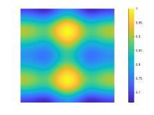
(b) $k=2$

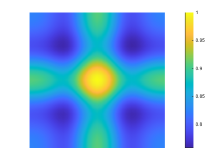
(c) $k=3$

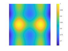
(d) $k=4$

Figure 7: The normalized amplitude of the x-component of the optimized patterns ${\bm{\theta}}_{k}({\bf s})$ with respect to ${\bf s}\in{\cal S}_{\rm T}$ for users $k=$1, 2, 3, and 4.

V-D Patterns ${\bm{\theta}}({\bf s})$ of CAP-MIMO

(a) $k=1$

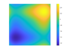
(b) $k=2$

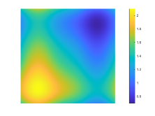
(c) $k=3$

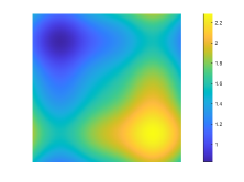
(d) $k=4$

Figure 8: The phase of the x-component of the optimized patterns ${\bm{\theta}}_{k}({\bf s})$ with respect to ${\bf s}\in{\cal S}_{\rm T}$ for users $k=$1, 2, 3, and 4.

To show the pattern functions optimized by the proposed pattern design scheme, by fixing $N_{F}=81$, we present the normalized amplitude of the x-component of the optimized patterns ${\bm{\theta}}_{k}({\bf s})$ for the former four users in Fig. 7, and their phase in Fig. 8, respectively. We observe from Fig. 7 that, after optimizing the patterns via the proposed scheme, the power of the patterns for different users are mainly distributed in non-overlapping regions, which seems like several orthogonal functions. It indicates that, in order to maximize the sum-rate, the pattern functions carrying different symbols are designed to be as orthogonal as possible to reduce the inter-user interference. Besides, from Fig. 8 one can notice that, the phase values of the patterns carrying different symbols are symmetrically distributed. It indicates that the information-carrying EM waves are steered toward the angular directions where the four users are located, respectively, as shown in Fig. 4. This interesting phenomenon is similar to the result of the conventional MIMO beamforming, which aims to generate spatially-orthogonal beams toward multiple users. We can conclude that, both of these two figures have provided intuitive explanations for the sum-rate improvement, which has also demonstrated the effectiveness of the proposed pattern design scheme.

V-E The Impact of User Positions on Sum-Rate

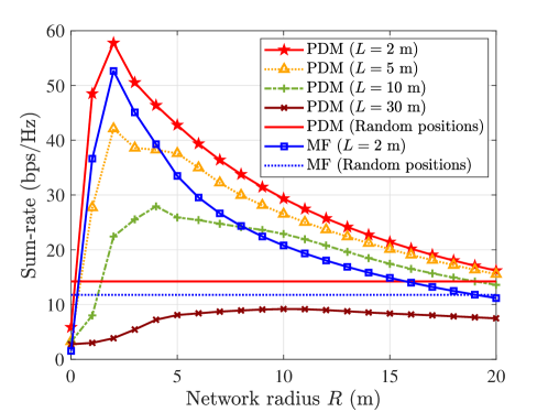
Figure 9: Sum-rate against the network radius $R$.

In this subsection, we show the impact of users’ positions on the sum-rate of a multi-user CAP-MIMO system. Specifically, we consider two different setups. Following the variable-controlling principle, for the first setup, we assume that the distances between all $K$ users and the transmitter’s center are equal. Thus, $K$ users are evenly located on a circle centered at $(0,0,L)$ with radius $R$, and the circle is parallel to the $xy$-plane. Particularly, the $k$-th user’s position is $\left(R{\rm cos}(\phi_{k}),R{\rm sin}(\phi_{k}),L\right)$ wherein $\phi_{k}=2k\pi/K$. Typically, we consider four different vertical distances $L=2\,{\rm m}$, $5\,{\rm m}$, $10\,{\rm m}$, $30\,{\rm m}$, and then simulate the sum-rate as a function of network radius $R$. For the second setup, we assume that the positions of $K$ users are randomly distributed in the volume ${\cal V}=\big{\{}R\in[2\,{\rm m},30\,{\rm m}],L\in[2\,{\rm m},30\,{\rm m}],\phi_{k}\in[0,2\pi],\forall k\in\{1,\cdots,K\}\big{\}}$ to account for the practical case. By fixing $N_{F}=81$, we plot the sum-rate as a function of network radius $R$ in Fig. 9, and we obtain the following two observations.

Firstly, the sum-rates for all schemes decrease as the vertical distance $L$ increases. For example, when $R=10\,{\rm m}$, the proposed PDM scheme can achieve the sum-rate of 29.32 bps/Hz, 26.51 bps/Hz, 22.90 bps/Hz, and 9.18 bps/Hz for $L=2\,{\rm m}$, $5\,{\rm m}$, $10\,{\rm m}$, and $30\,{\rm m}$, respectively. There are two reasons for this phenomenon. One reason is that, as the receivers get far away from the transmitter, more transmitted power is lost into space due to the larger-scale fading of channels, leading to a decrease in the signal strengths at the receivers. The other reason is that, limited by the spatial resolution of the CAP-MIMO aperture, the transmitter is increasingly difficult to accurately steer the desired signals toward the target positions.

Secondly, as the network radius $R$ increases, the sum-rate for each scheme experiences two stages: Increase to a peak at first and then gradually decrease at $R=2\,{\rm m}$. This interesting phenomenon can be explained as follows. During the first stage when $R$ is small, the users in the network are close, which results in serious inter-user interference. As $R$ increases, the interference gradually weakens, leading to an increasing sum-rate. Then, during the second stage, when $R$ is sufficiently large, the negative effect of large-scale channel fading becomes more significant, resulting in a decrease of the sum-rate.

VI Conclusions and Future Works

In this paper, we have developed PDM technique to design the CAP-MIMO patterns. Specifically, we have studied and modeled a multi-user CAP-MIMO system, which may provide a framework for some open problems, such as the analyses of channel DoFs and capacity [38]. The developed PDM is able to transform the design of the continuous pattern functions to the design of their projection lengths on finite orthogonal bases. Thus, PDM may serve as a signal processing framework for some technical problems in CAP-MIMO systems, such as channel estimation [17] and energy efficiency optimization [42]. Utilizing PDM, we have proposed a BCD based pattern design scheme to solve the formulated sum-rate maximization problem. Simulation results have shown that, the sum-rate achieved by the proposed scheme is higher than that achieved by benchmark schemes. In the future, the CAP-MIMO pattern design with lower complexity is important, and some modern tools like deep reinforcement learning [43] can be leveraged for the efficient pattern design of CAP-MIMO.

Appendix A Proof of Lemma 1

By integrating the radial component of the Poynting vector over a sphere with infinite-length radius, for a deterministic source in a given surface ${\cal S}_{\rm T}$, the physical radiation power can be upper-bounded by the integral of the Euclidean norm of ${\bf j}({\bf s})$ over ${\bf s}\in{\cal S}_{\rm T}$ [34]. Here we extend this proof to the case in the sense of expectation, where the current distribution ${\bf j}({\bf s})$ is a stochastic process composed of multiple patterns that carry symbols $\bf x$, as shown in (2).

Firstly, we calculate the Poynting vector $S({\bf{r}})$ by its definition:

$$S({\bf{r}})\!=\!\frac{1}{{2{Z_{0}}}}{\bf{e}}^{\rm H}({\bf{r}}){{\bf{e}}}({\bf{r}})$$

$$\!=\!\frac{1}{{2{Z_{0}}}}\!\sum\limits_{k=1}^{K}{{{\left|{{x_{k}}}\right|}^{2}}}{\left\|{\int_{{{\cal S}_{\rm{T}}}}{\bf{G}}({\bf{r}},{\bf{s}}){{\bm{\theta}}_{k}}\left({\bf{s}}\right){\rm{d}}{\bf{s}}}\right\|^{2}}+$$

$$\frac{1}{{2{Z_{0}}}}\!\sum\limits_{j\neq j^{\prime}}\!{x_{j}^{*}{x_{j^{\prime}}}{{\left({\int_{{{\cal S}_{\rm{T}}}}\!\!\!{\bf{G}}({\bf{r}},{\bf{s}}){{\bm{\theta}}_{j}}\left({\bf{s}}\right){\rm{d}}{\bf{s}}}\right)}^{\!\!\!\rm{H}}}\!{\int_{{{\cal S}_{\rm{T}}}}\!\!\!{\bf{G}}({\bf{r}},{\bf{s}}){{\bm{\theta}}_{j^{\prime}}}\left({\bf{s}}\right){\rm{d}}{\bf{s}}}},$$ (50)

where $\sum\nolimits_{j\neq j^{\prime}}\triangleq\sum\nolimits_{j^{\prime}=1}^{K}{\sum\nolimits_{j=1,j\neq j^{\prime}}^{K}{}}$. Utilizing ${\mathbb{E}}_{\bf x}\{{\bf x}{\bf x}^{\rm H}\}={\bf I}_{K}$, the physical radiation power of CAP-MIMO ${P_{{\rm{rad}}}}$ in the sense of expectation can be calculated as

$${P_{{\rm{rad}}}}= \mathop{\lim}\limits_{r\to\infty}{\mathbb{E}}_{\bf x}\left\{{\int_{{\Omega}}{S({\bf{r}}){r^{2}}}{\rm d}{\omega}}\right\}$$ (51)

$$= \mathop{\lim}\limits_{r\to\infty}\frac{1}{{2{Z_{0}}}}\sum\limits_{k=1}^{K}{\int_{\Omega}{{{\left\|{\int_{{{\cal S}_{\rm{T}}}}\!{\bf{G}}({\bf{r}},{\bf{s}}){{\bm{\theta}}_{k}}\left({\bf{s}}\right){\rm{d}}{\bf{s}}}\right\|}^{2}}{r^{2}}}{\rm d}\omega},$$

wherein $r=\left\|{\bf{r}}\right\|$ and $\omega\in\Omega$ is the solid angle of $4\pi$ steradians. Note that, when $r$ is large enough, the channel function ${\bf{G}}({\bf{r}},{\bf{s}})$ can be approximated by

$$\mathbf{G}(\mathbf{r},\mathbf{s})=\frac{{{\rm{j}}\kappa_{0}{{\rm{Z}}_{0}}}}{{4\pi}}\frac{{{e^{j\kappa_{0}r}}}}{r}\left({{\bf{I}}_{3}-\frac{{{\bf{r}}{{\bf{r}}^{\rm{H}}}}}{{{{r}^{2}}}}}\right){e^{-{\rm{j}}{{\bm{\kappa}}^{\rm T}}\left({\phi,\varphi}\right){\bf{s}}}},$$ (52)

where $\phi\in[0,\pi)$ and $\varphi\in[-\pi,\pi)$ are the elevation angle and azimuth angle respectively, which is associated with points $\bf r$ and $\bf s$. Plane-wave wave vector ${\bm{\kappa}}\left({\phi,\varphi}\right)$ takes the form of ${\bm{\kappa}}\left({\phi,\varphi}\right)=\frac{{2\pi}}{\lambda}{\left[{\cos\varphi\sin\phi,\sin\varphi\sin\phi,\cos\phi}\right]^{\rm{T}}}$. By substituting (52) into (51), we obtain

$${P_{{\rm{rad}}}}=$$

$$\mathop{\lim}\limits_{r\to\infty}\frac{{\kappa_{0}^{2}{{\rm{Z}}_{0}}}}{{32{\pi^{2}}}}\sum\limits_{k=1}^{K}{\int_{\Omega}{{{\left\|{\int_{{{\cal S}_{\rm{T}}}}\!\!{\left({{{\bf{I}}_{3}}\!-\!\frac{{{\bf{r}}{{\bf{r}}^{\rm{H}}}}}{{{r^{2}}}}}\right){e^{-{\rm{j}}{{\bm{\kappa}}^{\rm{T}}}\left({\phi,\varphi}\right){\bf{s}}}}}{{\bm{\theta}}_{k}}\left({\bf{s}}\right){\rm{d}}{\bf{s}}}\right\|}^{2}}}\!\!{\rm d}\omega}$$

$$\!\leq\!\mathop{\lim}\limits_{r\to\infty}\frac{{\kappa_{0}^{2}{{\rm{Z}}_{0}}}}{{32{\pi^{2}}}}\int_{\Omega}{\int_{{{\cal S}_{\rm{T}}}}{{{\left\|{\left({{{\bf{I}}_{3}}-\frac{{{\bf{r}}{{\bf{r}}^{\rm{H}}}}}{{{r^{2}}}}}\right){e^{-{\rm{j}}{{\bm{\kappa}}^{\rm{T}}}\left({\phi,\varphi}\right){\bf{s}}}}}\right\|}^{2}}}{\rm{d}}{\bf{s}}}{\rm d}\omega\times$$

$$~{}~{}~{}~{}~{}~{}~{}~{}~{}\sum\limits_{k=1}^{K}{\int_{{{\cal S}_{\rm{T}}}}{{{\left\|{{{\bm{\theta}}_{k}}\left({\bf{s}}\right)}\right\|}^{2}}}{\rm{d}}{\bf{s}}}$$ (53)

where Cauchy-Schwarz inequality is applied to the right side of the equality to derive its upper bound. It can be observed from (A) that, the component related to $r$ is limited when $r\to\infty$, i.e.,

$$0<\mathop{\lim}\limits_{r\to\infty}\int_{\Omega}{\int_{{{\cal S}_{\rm{T}}}}{{{\left\|{\left({{{\bf{I}}_{3}}-\frac{{{\bf{r}}{{\bf{r}}^{\rm{H}}}}}{{{r^{2}}}}}\right){e^{-{\rm{j}}{{\bm{\kappa}}^{\rm{T}}}\left({\phi,\varphi}\right){\bf{s}}}}}\right\|}^{2}}}{\rm{d}}{\bf{s}}}{\rm d}\omega<\infty.$$ (54)

Therefore, the physical radiation power of CAP-MIMO can be upper-bounded by the component in (A) unrelated to $r$, written as

$$\sum\limits_{k=1}^{K}{\int_{{{\cal S}_{\rm{T}}}}{{{\left\|{{{\bm{\theta}}_{k}}\left({\bf{s}}\right)}\right\|}^{2}}{\rm{d}}{\bf{s}}}}\leq{P_{\rm{T}}},$$ (55)

which completes the proof.

Appendix B Proof of Lemma 3

Obviously, the optimal solution to ${\cal P}_{s}$ in (22) is achieved when $\int_{{{\cal S}_{\rm{T}}}}{{{\left\|{{\bm{\theta}}\left({\bf{s}}\right)}\right\|}^{2}}{\rm{d}}{\bf{s}}}={P_{\rm{T}}}$. Thus, by applying Cauchy-Schwarz inequality for the objective of problem ${\cal P}_{s}$ in (22), we obtain

$$\gamma =\frac{{{{\left|{{{\bm{\psi}}^{\rm{H}}}\int_{{{\cal S}_{\rm{T}}}}{\bf{G}}({\bf{s}}){\bm{\theta}}\left({\bf{s}}\right){\rm{d}}{\bf{s}}}\right|}^{2}}}}{{{{\bm{\psi}}^{\rm{H}}}{\bm{\psi}}}{{\sigma^{2}}}}$$

$$\stackrel{{\scriptstyle(a)}}{{\leq}}\frac{{\left|{\int_{{{\cal S}_{\rm{T}}}}{{{\left\|{{{\bm{\psi}}^{\rm{H}}}{\bf{G}}({\bf{s}})}\right\|}^{2}}}{\rm{d}}{\bf{s}}}\right|\left|{\int_{{{\cal S}_{\rm{T}}}}{{{\left\|{{\bm{\theta}}\left({\bf{s}}\right)}\right\|}^{2}}}{\rm{d}}{\bf{s}}}\right|}}{{{{\bm{\psi}}^{\rm{H}}}{\bm{\psi}}}{{\sigma^{2}}}}$$

$$={P_{\rm{T}}}\frac{{\int_{{{\cal S}_{\rm{T}}}}{{{\left\|{{{\bm{\psi}}^{\rm{H}}}{\bf{G}}({\bf{s}})}\right\|}^{2}}}{\rm{d}}{\bf{s}}}}{{{{\bm{\psi}}^{\rm{H}}}{\bm{\psi}}}{{\sigma^{2}}}},$$ (56)

where equality $(a)$ holds when

$${\bm{\theta}}\left({\bf{s}}\right)=\sqrt{{P_{\rm{T}}}}\frac{{{{\bf{G}}^{\rm{H}}}({\bf{s}}){\bm{\psi}}}}{{\sqrt{\int_{{{\cal S}_{\rm{T}}}}{{{\left\|{{{\bf{G}}^{\rm{H}}}({\bf{s}}^{\prime}){\bm{\psi}}}\right\|}^{2}}{\rm{d}}{\bf{s}}^{\prime}}}}}$$ (57)

Thus, problem ${\cal P}_{s}$ in (22) can be equivalently reformulated as

$$\mathop{\max}\limits_{{\bm{\psi}}}~{}~{}\gamma ={P_{\rm{T}}}\frac{{\int_{{{\cal S}_{\rm{T}}}}{{{\left\|{{{\bm{\psi}}^{\rm{H}}}{\bf{G}}({\bf{s}})}\right\|}^{2}}}{\rm{d}}{\bf{s}}}}{{{{\bm{\psi}}^{\rm{H}}}{\bm{\psi}}}{{\sigma^{2}}}}$$

$$={P_{\rm{T}}}\frac{{{{\bm{\psi}}^{\rm{H}}}\left({\int_{{{\cal S}_{\rm{T}}}}{{{\bf{G}}}({\bf{s}}){\bf{G}}^{\rm{H}}({\bf{s}}){\rm{d}}{\bf{s}}}}\right){\bm{\psi}}}}{{{{\bm{\psi}}^{\rm{H}}}{\bm{\psi}}{\sigma^{2}}}}.$$ (58)

It is a standard Rayleigh quotient thus $\gamma$ can be maximized when combiner ${\bm{\psi}}$ takes the eigenvector corresponding to the maximum eigenvalue of matrix ${\int_{{{\cal S}_{\rm{T}}}}{{{\bf{G}}}({\bf{s}}){\bf{G}}^{\rm{H}}({\bf{s}}){\rm{d}}{\bf{s}}}}$, written as

$${\bm{\psi}}=\frac{{{\bm{\xi}}_{\max}}\left\{{\int_{{{\cal S}_{\rm{T}}}}{{{\bf{G}}}({\bf{s}}){\bf{G}}^{\rm{H}}({\bf{s}}){\rm{d}}{\bf{s}}}}\right\}}{\left\|{{\bm{\xi}}_{\max}}\left\{{\int_{{{\cal S}_{\rm{T}}}}{{{\bf{G}}}({\bf{s}}){\bf{G}}^{\rm{H}}({\bf{s}}){\rm{d}}{\bf{s}}}}\right\}\right\|}.$$ (59)

Then, the pattern design scheme in (24) can be obtained by substituting (59) into (57) and $\gamma^{\rm opt}$ in (23) can be obtained by substituting (24) into (22), which completes the proof.

Appendix C Proof of Lemma 4

For simplifying notations, here we define $\sum\nolimits_{{\bf{n}}={\bf{N}}+1}^{\infty}{}=\sum\nolimits_{\bf{n}}^{\infty}{}-\sum\nolimits_{\bf{n}}^{\bf{N}}{}$. Then, the full derivation process of Lemma 4 is summarized as follows.

Firstly, by substituting ${\gamma^{{\rm{opt}}}}$ in (25) and $\hat{\gamma}$ in (28) into $\Delta={{{\gamma^{{\rm{opt}}}}-\hat{\gamma}}}$, we obtain:

$$\Delta=\frac{2}{{{\sigma^{2}}}}{\Re}\left\{{{{\left({\sum\limits_{\bf{n}}^{\infty}{{{\bf{\Omega}}_{\bf{n}}}{{\bf{w}}_{\bf{n}}}}}\right)}^{\rm{H}}}\left({\sum\limits_{{\bf{n}}={\bf{N}}+1}^{\infty}{{{\bf{\Omega}}_{\bf{n}}}}{{\bf{w}}_{\bf{n}}}}\right)}\right\}-$$

$$~{}~{}~{}~{}~{}~{}~{}~{}~{}\frac{1}{{{\sigma^{2}}}}{\left\|{\sum\limits_{{\bf{n}}={\bf{N}}+1}^{\infty}{{{\bf{\Omega}}_{\bf{n}}}}{{\bf{w}}_{\bf{n}}}}\right\|^{2}}$$

$$\stackrel{{\scriptstyle(a)}}{{\leq}}\frac{2}{{{\sigma^{2}}}}\left\|{\sum\limits_{\bf{n}}^{\infty}{{{\bf{\Omega}}_{\bf{n}}}{{\bf{w}}_{\bf{n}}}}}\right\|\left\|{\sum\limits_{{\bf{n}}={\bf{N}}+1}^{\infty}{{{\bf{\Omega}}_{\bf{n}}}}{{\bf{w}}_{\bf{n}}}}\right\|-\frac{1}{{{\sigma^{2}}}}{\left\|{\sum\limits_{{\bf{n}}={\bf{N}}+1}^{\infty}{{{\bf{\Omega}}_{\bf{n}}}}{{\bf{w}}_{\bf{n}}}}\right\|^{2}}$$

$$\stackrel{{\scriptstyle(b)}}{{\leq}}\frac{1}{{{\sigma^{2}}}}\left\|{\sum\limits_{\bf{n}}^{\infty}{{{\bf{\Omega}}_{\bf{n}}}{{\bf{w}}_{\bf{n}}}}}\right\|\left\|{\sum\limits_{{\bf{n}}={\bf{N}}+1}^{\infty}{{{\bf{\Omega}}_{\bf{n}}}}{{\bf{w}}_{\bf{n}}}}\right\|+$$

$$~{}~{}~{}~{}~{}~{}~{}~{}~{}~{}~{}~{}~{}~{}~{}~{}~{}~{}~{}~{}~{}~{}\frac{1}{{{\sigma^{2}}}}\left\|{\sum\limits_{\bf{n}}^{\bf{N}}{{{\bf{\Omega}}_{\bf{n}}}{{\bf{w}}_{\bf{n}}}}}\right\|\left\|{\sum\limits_{{\bf{n}}={\bf{N}}+1}^{\infty}{{{\bf{\Omega}}_{\bf{n}}}}{{\bf{w}}_{\bf{n}}}}\right\|$$ (60)

where inequality $(a)$ follows since $\Re\left\{{{\bf{z}}^{\rm H}{\bf y}}\right\}\leq\left\|{\bf{z}}\right\|\left\|{\bf{y}}\right\|$ and $(b)$ follows since $\left\|{\bf{z}}\right\|-\left\|{\bf{y}}\right\|\leq\left\|{{\bf{z}}-{\bf{y}}}\right\|$. Then, by substituting ${{\bf{w}}_{\bf{n}}}$ in (26) as well as ${\bm{\theta}}({\bf s})$ and ${\bm{\psi}}$ in (24) into (C), we obtain:

$$\Delta\leq\frac{1}{{{\sigma^{2}}{A_{\rm{T}}}}}\frac{{{P_{\rm{T}}}}}{{\int_{{V_{s}}}{{{\left\|{{{\bf{G}}^{\rm{H}}}({\bf{s}}){\bm{\psi}}}\right\|}^{2}}d{\bf{s}}}}}\left\|{\int_{{{\cal S}_{\rm{T}}}}\!{\sum\limits_{\bf{n}}^{\infty}\!{{{\bf{\Omega}}_{\bf{n}}}}{\Psi_{\bf{n}}}({\bf{s}}){{\bf{G}}^{\rm{H}}}({\bf{s}}){\bm{\psi}}{\rm{d}}{\bf{s}}}}\right\|$$

$$\times\left\|{\int_{{{\cal S}_{\rm{T}}}}{\sum\limits_{{\bf{n}}={\bf{N}}+1}^{\infty}{{{\bf{\Omega}}_{\bf{n}}}}{\Psi_{\bf{n}}}({\bf{s}}){{\bf{G}}^{\rm{H}}}({\bf{s}}){\bm{\psi}}{\rm{d}}{\bf{s}}}}\right\|+$$

$$~{}~{}\frac{1}{{\sigma^{2}}{{A_{\rm{T}}}}}\frac{{{P_{\rm{T}}}}}{{\int_{{V_{s}}}{{{\left\|{{{\bf{G}}^{\rm{H}}}({\bf{s}}){\bm{\psi}}}\right\|}^{2}}d{\bf{s}}}}}\left\|{\int_{{{\cal S}_{\rm{T}}}}{\sum\limits_{\bf{n}}^{\bf{N}}{{{\bf{\Omega}}_{\bf{n}}}{\Psi_{\bf{n}}}({\bf{s}})}{{\bf{G}}^{\rm{H}}}({\bf{s}}){\bm{\psi}}{\rm{d}}{\bf{s}}}}\right\|\times$$

$$\left\|{\int_{{{\cal S}_{\rm{T}}}}{\sum\limits_{{\bf{n}}={\bf{N}}+1}^{\infty}{{{\bf{\Omega}}_{\bf{n}}}}{\Psi_{\bf{n}}}({\bf{s}}){{\bf{G}}^{\rm{H}}}({\bf{s}}){\bm{\psi}}{\rm{d}}{\bf{s}}}}\right\|.$$ (61)

Next, by utilizing Cauchy-Schwarz inequality $\left\|{\int_{{{\cal S}_{\rm{T}}}}{{\bf z}^{\rm H}{\bf{y}}{\rm d}{\bf{s}}}}\right\|\leq\sqrt{\int_{{{\cal S}_{\rm{T}}}}{{{\left\|{\bf{z}}\right\|}^{2}}{\rm d}{\bf{s}}}}\sqrt{\int_{{{\cal S}_{\rm{T}}}}{{{\left\|{\bf{y}}\right\|}^{2}}{\rm d}{\bf{s}}}}$, we further obtain

$$\Delta\leq$$

$$\frac{{{P_{\rm{T}}}}}{{{\sigma^{2}}{A_{\rm{T}}}}}\sqrt{\int_{{{\cal S}_{\rm{T}}}}{{{\left\|{\sum\limits_{\bf{n}}^{\infty}{{{\bf{\Omega}}_{\bf{n}}}}{\Psi_{\bf{n}}}({\bf{s}})}\right\|}^{2}}{\rm{d}}{\bf{s}}}}\sqrt{\int_{{{\cal S}_{\rm{T}}}}{{{\left\|{\sum\limits_{{\bf{n}}={\bf{N}}+1}^{\infty}\!\!\!{{{\bf{\Omega}}_{\bf{n}}}}{\Psi_{\bf{n}}}({\bf{s}})}\right\|}^{2}}\!{\rm{d}}{\bf{s}}}}$$

$$+\!\frac{{{P_{\rm{T}}}}}{{{\sigma^{2}}{A_{\rm{T}}}}}\sqrt{\int_{{{\cal S}_{\rm{T}}}}\!{{{\left\|{\sum\limits_{\bf{n}}^{\bf{N}}{{{\bf{\Omega}}_{\bf{n}}}{\Psi_{\bf{n}}}({\bf{s}})}}\right\|}^{2}}\!{\rm{d}}{\bf{s}}}}\sqrt{\int_{{{\cal S}_{\rm{T}}}}\!{{{\left\|{\sum\limits_{{\bf{n}}={\bf{N}}+1}^{\infty}\!\!\!{{{\bf{\Omega}}_{\bf{n}}}}{\Psi_{\bf{n}}}({\bf{s}})}\right\|}^{2}}\!{\rm{d}}{\bf{s}}}}$$

$$\stackrel{{\scriptstyle(a)}}{{\leq}}\frac{{{P_{\rm{T}}}}}{{{\sigma^{2}}}}\sqrt{\sum\limits_{\bf{n}}^{\infty}{{{\left\|{{{\bf{\Omega}}_{\bf{n}}}}\right\|}^{2}}}}\sqrt{\sum\limits_{{\bf{n}}={\bf{N}}+1}^{\infty}{{{\left\|{{{\bf{\Omega}}_{\bf{n}}}}\right\|}^{2}}}}+$$

$$~{}~{}~{}~{}~{}~{}~{}~{}~{}~{}~{}~{}~{}~{}~{}~{}\frac{{{P_{\rm{T}}}}}{{{\sigma^{2}}}}\sqrt{\sum\limits_{\bf{n}}^{\bf{N}}{{{\left\|{{{\bf{\Omega}}_{\bf{n}}}}\right\|}^{2}}}}\sqrt{\sum\limits_{{\bf{n}}={\bf{N}}+1}^{\infty}{{{\left\|{{{\bf{\Omega}}_{\bf{n}}}}\right\|}^{2}}}}.$$ (62)

where $(a)$ follows since $\left\|{\sum{\bf{z}}}\right\|\leq\sum{\left\|{\bf{z}}\right\|}$. Finally, the upper bound of $\Delta$ can be derived as

$$\Delta\stackrel{{\scriptstyle(a)}}{{\leq}} \frac{{{P_{\rm{T}}}}}{{{\sigma^{2}}}}\sqrt{\sum\limits_{\bf{n}}^{\infty}{\left\|{{{\bf{\Omega}}_{\bf{n}}}}\right\|_{\rm{F}}^{2}}}\sqrt{\sum\limits_{{\bf{n}}={\bf{N}}+1}^{\infty}{\left\|{{{\bf{\Omega}}_{\bf{n}}}}\right\|_{\rm{F}}^{2}}}+$$

$$~{}~{}~{}~{}~{}~{}~{}~{}\frac{{{P_{\rm{T}}}}}{{{\sigma^{2}}}}\sqrt{\sum\limits_{\bf{n}}^{\bf{N}}{\left\|{{{\bf{\Omega}}_{\bf{n}}}}\right\|_{\rm{F}}^{2}}}\sqrt{\sum\limits_{{\bf{n}}={\bf{N}}+1}^{\infty}{\left\|{{{\bf{\Omega}}_{\bf{n}}}}\right\|_{\rm{F}}^{2}}}$$

$$\stackrel{{\scriptstyle(b)}}{{=}} \frac{{{P_{\rm{T}}}}}{{{\sigma^{2}}}}\sqrt{\sum\limits_{\bf{n}}^{\infty}{\left\|{{{\bf{\Omega}}_{\bf{n}}}}\right\|_{\rm{F}}^{2}}}\sqrt{\left({1-\eta}\right)\sum\limits_{\bf{n}}^{\infty}{\left\|{{{\bf{\Omega}}_{\bf{n}}}}\right\|_{\rm{F}}^{2}}}+$$

$$~{}~{}~{}~{}~{}~{}~{}~{}\frac{{{P_{\rm{T}}}}}{{{\sigma^{2}}}}\sqrt{\eta\sum\limits_{\bf{n}}^{\infty}{\left\|{{{\bf{\Omega}}_{\bf{n}}}}\right\|_{\rm{F}}^{2}}}\sqrt{\left({1-\eta}\right)\sum\limits_{\bf{n}}^{\infty}{\left\|{{{\bf{\Omega}}_{\bf{n}}}}\right\|_{\rm{F}}^{2}}}$$

$$\stackrel{{\scriptstyle(c)}}{{=}} \frac{{{P_{\rm{T}}}}}{{{\sigma^{2}}}}\sqrt{1-\eta}\left({1+\sqrt{\eta}}\right)\int_{{{\cal S}_{\rm T}}}{\left\|{{\bf{G}}({\bf{s}})}\right\|_{\rm{F}}^{2}{\rm d}{\bf{s}}},$$ (63)

where $(a)$ follows since $\left\|{\bf{z}}\right\|\leq{\left\|{\bf{z}}\right\|_{\rm{F}}}$; $(b)$ holds since $\eta={{\sum\nolimits_{\bf{n}}^{\bf{N}}{\left\|{{{\bf{\Omega}}_{\bf{n}}}}\right\|_{\rm{F}}^{2}}}\mathord{\left/{\vphantom{{\sum\limits_{\bf{n}}^{\bf{N}}{\left\|{{{\bf{\Omega}}_{\bf{n}}}}\right\|_{\rm{F}}^{2}}}{\sum\limits_{\bf{n}}^{\infty}{\left\|{{{\bf{\Omega}}_{\bf{n}}}}\right\|_{\rm{F}}^{2}}}}}\right.\kern-1.2pt}{\sum\nolimits_{\bf{n}}^{\infty}{\left\|{{{\bf{\Omega}}_{\bf{n}}}}\right\|_{\rm{F}}^{2}}}}$; and $(c)$ holds according to Parseval’s theorem shown in (18). This completes the proof.

Zijian Zhang (Student Member, IEEE) received the B.E. degree in electronic engineering from Tsinghua University, Beijing, China, in 2020. He is currently working toward the Ph.D. degree in electronic engineering from Tsinghua University, Beijing, China. His research interests include physical-layer algorithms for massive MIMO, holographic MIMO (H-MIMO), and reconfigurable intelligent surfaces (RIS). He is also an amateur in wireless localization and robotics. He has authored or coauthored several journal and conference papers for the IEEE Journal on Selected Areas in Communications, the IEEE Transactions on Signal Processing, the IEEE Transactions on Wireless Communications, the IEEE Transactions on Communications, the IEEE ICC, the IEEE GLOBECOM, etc. He has received the National Scholarship in 2019 and the Excellent Thesis Award of Tsinghua University in 2020.

Linglong Dai (Fellow, IEEE) received the B.S. degree from Zhejiang University, Hangzhou, China, in 2003, the M.S. degree (with the highest honor) from the China Academy of Telecommunications Technology, Beijing, China, in 2006, and the Ph.D. degree (with the highest honor) from Tsinghua University, Beijing, China, in 2011. From 2011 to 2013, he was a Postdoctoral Research Fellow with the Department of Electronic Engineering, Tsinghua University, where he was an Assistant Professor from 2013 to 2016, an Associate Professor since from 2016 to 2022, and has been a Professor since 2022. His current research interests include massive MIMO, reconfigurable intelligent surface (RIS), millimeter-wave and Terahertz communications, machine learning for wireless communications, and electromagnetic information theory. He has authored or coauthored over 80 IEEE journal articles and over 50 IEEE conference papers. He also holds 19 granted patents. He has coauthored the book MmWave Massive MIMO: A Paradigm for 5G (Academic Press, 2016). He has received five IEEE Best Paper Awards at the IEEE ICC 2013, the IEEE ICC 2014, the IEEE ICC 2017, the IEEE VTC 2017-Fall, and the IEEE ICC 2018. He has also received the Tsinghua University Outstanding Ph.D. Graduate Award in 2011, the Beijing Excellent Doctoral Dissertation Award in 2012, the China National Excellent Doctoral Dissertation Nomination Award in 2013, the URSI Young Scientist Award in 2014, the IEEE Transactions on Broadcasting Best Paper Award in 2015, the Electronics Letters Best Paper Award in 2016, the National Natural Science Foundation of China for Outstanding Young Scholars in 2017, the IEEE ComSoc Asia Pacific Outstanding Young Researcher Award in 2017, the IEEE ComSoc Asia-Pacific Outstanding Paper Award in 2018, the China Communications Best Paper Award in 2019, IEEE Access Best Multimedia Award in 2020, the IEEE Communications Society Leonard G. Abraham Prize in 2020, and the IEEE ComSoc Stephen O. Rice Prize in 2022, and the IEEE ICC Outstanding Demo Award in 2022. He was listed as a Highly Cited Researcher by Clarivate Analytics from 2020 to 2022. He was elevated as an IEEE Fellow in 2022. He is currently serving as an Area Editor of the IEEE Communications Letters, and an Editor of the IEEE Transactions on Wireless Communications. He has also served as an Editor of the IEEE Transactions on Communications (2017-2021), an Editor of the IEEE Transactions on Vehicular Technology (2016-2020), and an Editor of the IEEE Communications Letters (2016-2020). He has also served as a Guest Editor of the IEEE Journal on Selected Areas in Communications, IEEE Journal of Selected Topics in Signal Processing, IEEE Wireless Communications, etc. Particularly, he is dedicated to reproducible research and has made a large amount of simulation code publicly available.

References

• [1] Z. Zhang and L. Dai, “Pattern-division multiplexing for continuous-aperture MIMO,” in Proc. 2022 IEEE Int. Conf. Commun. (IEEE ICC’22), May 2022, pp. 1–6.
• [2] J. G. Andrews, S. Buzzi, W. Choi, S. V. Hanly, A. Lozano, A. C. K. Soong, and J. C. Zhang, “What will 5G be?” IEEE J. Sel. Areas Commun., vol. 32, no. 6, pp. 1065–1082, Jun. 2014.
• [3] F. Boccardi, R. W. Heath, A. Lozano, T. L. Marzetta, and P. Popovski, “Five disruptive technology directions for 5G,” IEEE Commun. Mag., vol. 52, no. 2, pp. 74–80, Feb. 2014.
• [4] J. G. Andrews, X. Zhang, G. D. Durgin, and A. K. Gupta, “Are we approaching the fundamental limits of wireless network densification?” IEEE Commun. Mag., vol. 54, no. 10, pp. 1558–1896, Oct. 2016.
• [5] L. Lu, G. Y. Li, A. L. Swindlehurst, A. Ashikhmin, and R. Zhang, “An overview of massive MIMO: Benefits and challenges,” IEEE J. Sel. Topics Signal Process., vol. 8, no. 5, pp. 742–758, Oct. 2014.
• [6] Y. Sun, Z. Gao, H. Wang, B. Shim, G. Gui, G. Mao, and F. Adachi, “Principal component analysis-based broadband hybrid precoding for millimeter-wave massive MIMO systems,” IEEE Trans. Wireless Commun., vol. 19, no. 10, pp. 6331–6346, Oct. 2020.
• [7] C. Feng, W. Shen, J. An, and L. Hanzo, “Weighted sum rate maximization of the mmwave cell-free MIMO downlink relying on hybrid precoding,” IEEE Trans. Wireless Commun., Sep. 2021.
• [8] Ö. Demir, E. Björnson, and L. Sanguinetti, “Channel modeling and channel estimation for holographic massive MIMO with planar arrays,” IEEE Wireless Commun. Lett., Feb. 2022.
• [9] M. Ghermezcheshmeh, V. Jamali, H. Gacanin, and N. Zlatanov, “Parametric channel estimation for LoS dominated holographic massive MIMO systems,” arXiv preprint arXiv:2112.02874, Dec. 2021.
• [10] A. Pizzo, T. L. Marzetta, and L. Sanguinetti, “Spatially-stationary model for holographic MIMO small-scale fading,” IEEE J. Sel. Areas Commun., vol. 38, no. 9, pp. 1964–1979, Sep. 2020.
• [11] N. Decarli and D. Dardari, “Communication modes with large intelligent surfaces in the near field,” IEEE Access, vol. 9, pp. 165 648–165 666, Dec. 2021.
• [12] L. Sanguinetti, A. A. D’Amico, and M. Debbah, “Wavenumber-division multiplexing in line-of-sight holographic MIMO communications,” IEEE Trans. Wireless Commun., Sep. 2022.
• [13] D. Dardari, “Communicating with large intelligent surfaces: Fundamental limits and models,” IEEE J. Sel. Areas Commun., vol. 38, no. 11, pp. 2526–2537, Nov. 2020.
• [14] A. Pizzo, L. Sanguinetti, and T. L. Marzetta, “Fourier plane-wave series expansion for holographic MIMO communications,” IEEE Trans. Wireless Commun., Mar. 2022.
• [15] S. Hu, F. Rusek, and O. Edfors, “Beyond massive MIMO: The potential of data transmission with large intelligent surfaces,” IEEE Trans. Signal Process., vol. 66, no. 10, pp. 2746–2758, May 2018.
• [16] J. Yuan, H. Q. Ngo, and M. Matthaiou, “Towards large intelligent surface (LIS)-based communications,” IEEE Trans. Commun., vol. 68, no. 10, pp. 6568–6582, Oct. 2020.
• [17] C. Huang, S. Hu, G. C. Alexandropoulos, A. Zappone, C. Yuen, R. Zhang, M. D. Renzo, and M. Debbah, “Holographic MIMO surfaces for 6G wireless networks: Opportunities, challenges, and trends,” IEEE Wireless Commun., vol. 27, no. 5, pp. 118–125, Oct. 2020.
• [18] Z. Wang, Z. Liu, Y. Shen, A. Conti, and M. Z. Win, “Location awareness in beyond 5G networks via reconfigurable intelligent surfaces,” IEEE J. Sel. Areas Commun., Mar. 2022.
• [19] Z. Wan, Z. Gao, F. Gao, M. D. Renzo, and M.-S. Alouini, “Terahertz massive MIMO with holographic reconfigurable intelligent surfaces,” IEEE Trans. Commun., vol. 69, no. 7, pp. 4732–4750, Jul. 2021.
• [20] S. Maci, G. Minatti, M. Casaletti, and M. Bosiljevac, “Metasurfing: Addressing waves on impenetrable metasurfaces,” IEEE Antennas Wireless Propag. Lett., vol. 10, pp. 1499–1502, 2011.
• [21] J. Hunt, J. Gollub, T. Driscoll, G. Lipworth, A. Mrozack, M. Reynolds, D. Brady, and D. Smith, “Metamaterial microwave holographic imaging system,” J. Opt. Soc. Amer. A, Opt. Image Sci., vol. 31, no. 10, p. 2109–2119, Jul. 2014.
• [22] D. González-Ovejero, G. Minatti, G. Chattopadhyay, and S. Maci, “Multibeam by metasurface antennas,” IEEE Trans. Antennas Propag., vol. 65, no. 6, pp. 2923–2930, Jun. 2017.
• [23] O. Yurduseven, D. L. Marks, T. Fromenteze, and D. R. Smith, “Dynamically reconfigurable holographic metasurface aperture for a mills-cross monochromatic microwave camera,” Opt. Express, vol. 26, no. 5, p. 5281–5291, Feb. 2018.
• [24] R.-B. R. Hwang, “Binary meta-hologram for a reconfigurable holographic metamaterial antenna,” Sci. Rep., vol. 10, no. 1, pp. 1–10, May 2020.
• [25] M. E. Badawe, T. S. Almoneef, and O. M. Ramahi, “A true metasurface antenna,” Sci. Rep., vol. 6, no. 1, pp. 1–8, Jan. 2016.
• [26] Q. Hu, K. Chen, N. Zhang, J. Zhao, T. Jiang, J. Zhao, and Y. Feng, “Arbitrary and dynamic poincaré sphere polarization converter with a time-varying metasurface,” Adv. Opt. Mater., vol. 10, no. 4, p. 2101915, Apr. 2022.
• [27] W. Jeon and S.-Y. Chung, “The capacity of wireless channels: A physical approach,” in Proc. 2013 IEEE Int. Symposium Inf. Theory (IEEE ISIT’13), Jul. 2013, pp. 3045–3049.
• [28] H. Wheeler, “Simple relations derived fom a phased-array antenna made of an infinite current sheet,” IEEE Trans. Antennas Propag., vol. 13, no. 4, pp. 506–514, Jul. 1965.
• [29] D. Staiman, M. Breese, and W. Patton, “New technique for combining solid-state sources,” IEEE J. Solid-State Circuits, vol. 3, no. 3, pp. 238–243, Sep. 1968.
• [30] D. A. Miller, “Communicating with waves between volumes: evaluating orthogonal spatial channels and limits on coupling strengths,” Applied Optics, vol. 39, no. 11, pp. 1681–1699, Nov. 2000.
• [31] M. A. Jensen and J. W. Wallace, “Capacity of the continuous-space electromagnetic channel,” IEEE Trans. Antennas Propag., vol. 56, no. 2, pp. 524–531, Feb. 2008.
• [32] L. Wei, C. Huang, G. Alexandropoulus, E. Wei, Z. Zhang, M. Debbah, and C. Yuen, “Multi-user holographic MIMO surfaces: Channel modeling and spectral efficiency analysis,” IEEE J. Sel. Topics Signal Process., 2022.
• [33] D. O’Regan and G. Teobaldi, “Optimization of constrained density functional theory,” Physical Review B, vol. 94, Mar. 2016.
• [34] F. K. Gruber and E. A. Marengo, “New aspects of electromagnetic information theory for wireless and antenna systems,” IEEE Trans. Antennas Propag., vol. 56, no. 11, pp. 3470–3484, Nov. 2008.
• [35] N. Fatema, G. Hua, Y. Xiang, D. Peng, and I. Natgunanathan, “Massive MIMO linear precoding: A survey,” IEEE Sys. J., vol. 12, no. 4, pp. 3920–3931, Dec. 2018.
• [36] H. Li, Z. Zhou, Y. He, W. Sun, Y. Li, I. Liberal, and N. Engheta, “Geometry-independent antenna based on epsilon-near-zero medium,” Nat. Commun., vol. 13, no. 1, pp. 1–8, 2022.
• [37] K. Shen and W. Yu, “Fractional programming for communication systems—part I: Power control and beamforming,” IEEE Trans. Signal Process., vol. 66, no. 10, pp. 2616–2630, May 2018.
• [38] Z. Wan, J. Zhu, Z. Zhang, and L. Dai, “Capacity for electromagnetic information theory,” arXiv preprint arXiv:2111.00496, Nov. 2021.
• [39] D. Donoho, “Compressed sensing,” IEEE Trans. Inf. Theory, vol. 52, no. 4, pp. 1289–1306, Apr. 2006.
• [40] Q. Shi, M. Razaviyayn, Z.-Q. Luo, and C. He, “An iteratively weighted MMSE approach to distributed sum-utility maximization for a MIMO interfering broadcast channel,” IEEE Trans. Signal Process., vol. 59, no. 9, pp. 4331–4340, Sep. 2011.
• [41] S. Boyd, N. Parikh, E. Chu, B. Peleato, and J. Eckstein, “Distributed optimization and statistical learning via the alternating direction method of multipliers,” Nov. 2014, [Online] Available: https://stanford.edu/~boyd/papers/pdf/admm_distr_stats.pdf.
• [42] C. Huang, A. Zappone, G. C. Alexandropoulos, M. Debbah, and C. Yuen, “Reconfigurable intelligent surfaces for energy efficiency in wireless communication,” IEEE Trans. Wireless Commun., vol. 18, no. 8, pp. 4157–4170, Aug. 2019.
• [43] C. Huang, R. Mo, and C. Yuen, “Reconfigurable intelligent surface assisted multiuser MISO systems exploiting deep reinforcement learning,” IEEE J. Sel. Areas Commun., vol. 38, no. 8, pp. 1839–1850, Jun. 2020.