Sensing the shape of a cell with reaction-diffusion and energy minimization

Abstract

Some dividing cells sense their shape by becoming polarized along their long axis. Cell polarity is controlled in part by polarity proteins like Rho GTPases cycling between active membrane-bound forms and inactive cytosolic forms, modeled as a “wave-pinning” reaction-diffusion process. Does shape sensing emerge from wave-pinning? We show that wave pinning senses the cell’s long axis. Simulating wave-pinning on a curved surface, we find that high-activity domains migrate to peaks and troughs of the surface. For smooth surfaces, a simple rule of minimizing the domain perimeter while keeping its area fixed predicts the final position of the domain and its shape. However, when we introduce roughness to our surfaces, shape sensing can be disrupted, and high-activity domains can become localized to locations other than the global peaks and valleys of the surface. On rough surfaces, the domains of the wave-pinning model are more robust in finding the peaks and troughs than the minimization rule, though both can become trapped in steady states away from the peaks and valleys. We can control the robustness of shape sensing by altering the Rho GTPase diffusivity and the domain size. We also find that the shape sensing properties of cell polarity models can explain how domains localize to curved regions of deformed cells. Our results help to understand the factors that allow cells to sense their shape – and the limits that membrane roughness can place on this process.

For cells to respond to changing environments Doyle et al. (2013); Baker and Chen (2012) by choosing a direction to crawl, an axis of division, or a location to form a new branch, they must develop an internal biochemical polarity, where proteins are distributed inhomogeneously around the cell surface. In addition, the shape of the cell and its internal membranes can help organize its polarity – cells can sense their own shape Haupt and Minc (2018). Localization of different proteins to different regions can occur when individual proteins prefer to bind to membranes that have a specified curvature range, as is known to happen with BAR proteins  Simunovic et al. (2016); Peter et al. (2004), ArfGAP Bigay et al. (2005); Drin et al. (2007); Vanni et al. (2014), $\alpha$-synuclein  Pranke et al. (2011) SpoVM Levin et al. (1993) and septins Mostowy and Cossart (2012). However, even if individual proteins do not have a curvature preference, reactions on a cell membrane can be sensitive to the shape of that membrane, leading to patterns of protein localization sensitive to the membrane’s shape. This is the broadest idea of “shape sensing.” This shape sensitivity can arise from the local changes in surface-to-volume ratio Meyers et al. (2006) or more complicated reaction-diffusion mechanisms Camley et al. (2017); Cusseddu et al. (2019); Rangamani et al. (2013); Ramirez et al. (2015); Frank et al. (2019); Spill et al. (2016); Eroumé et al. (2021). Experiments have measured key correlations between localization of myosin II Elliott et al. (2015), and PIP₂ Driscoll et al. (2019) and local cell shape features like curvature, while inducing curvature within a cell can change the localization of both myosin II Elliott et al. (2015) and the polarity protein Rho Wigbers et al. (2021). Yeast polarity domain size also reflects cell shape Bonazzi et al. (2015). Bacterial shape sensing has also been recapitulated in vitro for the Min system of E. coli Schweizer et al. (2012); Halatek and Frey (2014). Shape sensing may also play a role in creating instabilities where cells crawl in circles Camley et al. (2017); Allen et al. (2020) or have a periodic motion Camley et al. (2013). Even the existence of polarization is sensitive to cell volume Hubatsch et al. (2019). Most dramatically, recent work studying the distribution of PAR proteins in the C. elegans zygote demonstrates a clear binary shape sensing: when PAR proteins are disrupted from their natural location by experimental intervention, they return to become localized to the nearest narrow end of the zygote  Mittasch et al. (2018). This experiment demonstrates that PAR proteins sense the long axis of the cell – while not establishing whether this sensing is self-organized, or arises from a pre-existing pattern.

Some elements of shape sensing are well understood, e.g. how patterns can be selected by controlling the possible wavelengths of an initial linear instability Murray (2001). Here we focus on a specific aspect of shape sensing: motivated by Mittasch et al. (2018), we study how a single initial domain of high concentration moves in response to the shape of its membrane. We will refer to this as “domain migration shape sensing,” to distinguish it from other examples of sensitivity to shape mentioned earlier. Domain migration cannot be captured by linear stability analysis, and is not well understood. As a prototype model, we study a minimal model of cell polarity, the “wave-pinning” (WP) model of Mori et al. Mori et al. (2008) which describes Rho GTPase dynamics. We use this model as the simplest model that robustly describes cell polarity, but it is also closely related to more detailed models used to describe PAR protein dynamics Goehring et al. (2011a). Previous work has shown that membrane-bound active form of Rho GTPases localize to the narrow end of the cell Jilkine (2009); Vanderlei et al. (2011); Camley et al. (2017), and links between the wave pinning model and the Allen-Cahn model have been suggested Jilkine (2009); Mori et al. (2011). These behaviors occur not only in the basic wave pinning model but also in significantly more complicated models including multiple Rho GTPases and phosphoinositides Marée et al. (2012, 2006). Later work has also shown that narrow-end localization occurs in three dimensions, but also demonstrates that domain localization in response to a complex cell shape is difficult to predict Cusseddu et al. (2019).

Can we reproduce the shape sensing via domain migration of Mittasch et al. (2018) using a simple model? Is there a predictive minimal theory for where polarity proteins will end up in a cell, other than just solving the complex reaction-diffusion PDEs? Previous simulation work has also focused on smooth, idealized surfaces. Would reaction-diffusion mechanisms for shape sensing be robust to the rough, complex shapes observed in real cells? In this paper, we study these questions. We find that a minimal WP model is able to recapitulate binary shape sensing as well as localization of domains to corners of triangular cells. We also argue that in many cases, we can understand the dynamics of complex domain shapes arising from the WP model by minimizing domain perimeter while keeping domain area fixed. However, we find that this simple minimization principle can be disrupted in sufficiently rough membrane geometries, where shape sensing itself is also less reliable. We show that shape sensing can be modulated by altering the diffusion coefficient of the membrane-bound form of our Rho GTPase, as well as the domain area. Our work is a systematic test of a minimal theory for how shape influences Rho GTPase cell polarity, and provides an understanding of when shape sensing will succeed depending on the cell geometry.

Figure 1: (a) A schematic of the reaction involved in the wave-pinning (WP) model. In the inactive form, Rho GTPases are in the cytosol, $\rho_{\textrm{cytosolic}}$. The active form $\rho$ is in the membrane. There is a positive feedback: presence of the active form on the membrane locally promotes conversion from the inactive form. (b) Representation of a domain in the perimeter minimization (PM) model. The red curve lies in a 3D surface. Its projection on the $x$-$y$ plane is shown as the black curve. To calculate the length of the boundary and the surface area enclosed by the red curve, we divide the black curve into triangles as shown and use results from differential geometry (Appendix).

I Models

I.1 Wave-pinning model of cell polarity

We describe cell polarity with a variant of the wave-pinning (WP) reaction-diffusion system Mori et al. (2008). This model treats Rho GTPases exchanging between the active membrane-bound $\rho({\mathbf{r}})$ and inactive cytosolic $\rho_{\textrm{cytosolic}}$ states with rate $f(\rho,\rho_{\textrm{cytosolic}})$, and the membrane-bound form diffusing on the curved membrane with diffusion coefficient $D$; the total amount of Rho GTPase is conserved. $\rho({\mathbf{r}})$ obeys the reaction-diffusion equation:

$$\partialderivative{\rho}{t} =D\laplacian\rho+f(\rho,\rho_{\mathrm{cytosolic}}).$$ (1)

The reaction term $f(\rho,\rho_{\mathrm{cytosolic}})$ includes basal rates of activation, de-activation, and a positive feedback where activation occurs more often when active Rho GTPase is already present:

$$f(\rho,\rho_{\mathrm{cytosolic}})=\rho_{\mathrm{cytosolic}}\left(k_{0}+\frac{\gamma\rho^{2}}{K^{2}+\rho^{2}}\right)-\delta\rho$$ (2)

where $k_{0}$ is a basal rate of activation, $K$ is the concentration at which the positive feedback begins to saturate, and $\gamma$ is the maximal rate of activation from positive feedback. The basal rate of the reverse reaction i.e. conversion from $\rho$ to $\rho_{\mathrm{cytosolic}}$ is $\delta$. In all the results presented in this paper, we have used $k_{0}=0.07$ s^-1, $\gamma=5$ s^-1, $K=2$ $\mu\mathrm{m}^{-2}$, and $\delta=3$ s^-1. Unless otherwise stated, we use $D=0.5\ \mu\mathrm{m}^{2}\mathrm{s}^{-1}$. The order of magnitude of these quantities are based on Mori et al. (2008).

We assume that the diffusion coefficient of the cytosolic form is so much larger than the diffusion coefficient of $\rho$ that $\rho_{\mathrm{cytosolic}}$ is well-mixed, i.e. constant over the cell volume. Because of the conservation of Rho GTPases between the membrane-bound and cytosolic forms, the total number of Rho GTPase proteins is $\int_{\textrm{membrane}}\rho+\int_{\textrm{cytosol}}\rho_{\textrm{cytosol}}$, which is a unitless constant we call $M$. We can then determine $\rho_{\textrm{cytosolic}}$ as:

$$\rho_{\mathrm{cytosolic}} =\frac{M}{\omega S}-\frac{1}{\omega S}\int_{\mathrm{membrane}}\rho.$$ (3)

$S$ denotes the surface area of the cell. $\omega$ is the ratio of the volume of the cell to its surface area. Thus, $\omega S$ is the volume of the cell. When we simulate an abstract surface $h(x,y)$ where there is no clear cytosolic volume, we take $\omega=1\,\muup\textrm{m}$. We choose $M/S=2.9\mu m^{-2}$ as a default value in our simulations; changing this value changes the size of the domain of high Rho GTPase activity, and if it is increased or decreased too much, it will prevent the cell from polarizing. The equation Eq. 1 is solved on our curved surfaces using a finite element method (Appendix).

Figure 2: The WP model is able to reproduce the shape sensing behavior of PAR proteins. (a) Top view: High concentration domains that were created away from the ends travel towards the ends over a duration of several minutes. Note that we initialize the domain at a size a little smaller than its steady-state size; it first expands and then migrates. (b) Front view: the angular position of the center of mass of a high-concentration domain from the vertical axis. (c) the final angular position of the domain center of mass as a function of the inital angular position. The steady state “flips” when $\theta$ crosses $\pi$. This is analogous to the binary shape sensing of Mittasch et al. (2018).

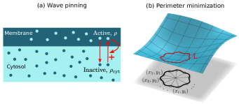
When parameters allow polarization (see, e.g. Mori et al. (2008); Camley et al. (2013); Mori et al. (2011)), the WP model reaction-diffusion equation Eq. 1 admits solutions that have a high-concentration region with $\rho\approx\rho^{+}$ and low-concentration regions of $\rho\approx\rho_{-}$. These values are set by the roots of $f(\rho,\rho_{\textrm{cytosolic}})=0$, which are, when the system allows polarization, $\rho_{-},\rho_{0}$, and $\rho_{+}$, in increasing order. An initial domain of enriched $\rho$ will evolve into a “pinned” state, where it has an area set by the reaction kinetics, the geometry, and the total amount of Rho GTPase $M$. The conditions for pinning, which set the steady-state domain shape in terms of the total amount $M$ and the values $\rho_{-}$ and $\rho_{+}$ are discussed in Mori et al. (2008, 2011); Camley et al. (2013). After the formation of a stable pinned domain, the domain moves over the surface, keeping its area roughly constant. On a flat two-dimensional surface, Jilkine has used asymptotic analysis to show that the velocity of the domain edge is is proportional to its curvature Jilkine (2009), tending to minimize the perimeter.

I.2 Perimeter minimization model

On a flat surface, solutions of the wave-pinning equations tend to minimize their domain perimeter Jilkine (2009), but their area remains roughly constant, suggesting that the dynamics of domains in these reaction-diffusion systems may be captured by minimizing perimeter while keeping area constant. This same idea may also capture more general proposed mechanisms for cell polarity, like binary mixture phase separation Orlandini et al. (2013); Semplice et al. (2012). In these models, line tension between the two phases drives domain coalescence and coarsening to minimize interface tension, while mass conservation keeps domain area fixed. Thus, both wave-pinning and phase separation pictures of cellular polarization tend to minimize the interface length of a polarity protein domain. Therefore, we will also study a perimeter minimization (PM) model of cell polarity. In the perimeter minimization model, the high $\rho$ concentration domain is represented by a portion of the 3D surface bounded by a closed curve that lies in the surface (Fig. 1b). The closed curve is the boundary of the domain. We minimize the length of the boundary while constraining the enclosed surface area to be fixed. The domain is free to relocate on the underlying surface.

To calculate the length of the boundary and the enclosed area, we project the 3D curve to the $x$-$y$ plane, as shown in Fig. 1. The projected curve is divided into triangular “pie slices”. Given the surface $h(x,y)$ and the points $\{x_{i},y_{i}\}$ defining the domain we can compute the domain’s perimeter $L\left(\{x_{i},y_{i}\}\right)$ and area $A\left(\{x_{i},y_{i}\}\right)$ on the surface using the first fundamental form of the surface and Gaussian quadrature (see Appendix). We chose this approach to allow for simple differentiation of the energy. We have argued that we should expect many polarity mechanisms to minimize the domain perimeter while keeping domain area fixed. To numerically find these minima, we minimize the energy

$$\mathcal{F}\left(\{x_{i},y_{i}\}\right)=L\left(\{x_{i},y_{i}\}\right)+\frac{1}{2}k\left(A\left(\{x_{i},y_{i}\}\right)-A_{0}\right)^{2}$$ (4)

Eq. 4 penalizes deviations away from the prescribed area $A_{0}$ with a coefficient $k=10^{3}\mu\mathrm{m}^{-1}$ as a strong area constraint. (We find that with this value of $k$, steady-state areas are well-constrained to $A_{0}$ to within about 2%). We choose $A_{0}$ to be the average steady state area of high concentration domains in WP simulations for the given surface. The parameter $A_{0}$ will also depend on the total amount of protein $M$, because this will alter the steady-state domain size. Values of $A_{0}$ for each simulation are provided in Table S1 in the Appendix.

We assume that the domain evolves in an overdamped way, i.e. the velocity of a point $(x_{i},y_{i})$ is negatively proportional to the gradient of the energy $\mathcal{F}$. The overdamped dynamics assumption here is a minimal one; more complex models that still minimize the energy would also be possible Hohenberg and Halperin (1977), e.g. modeling how the membrane lipids flow in response to deformations of a domain with a line tension Camley and Brown (2010). The overdamped dynamics corresponds to minimizing $\mathcal{F}$ using a simple gradient-descent algorithm. Thus, we generate a series of $\{x_{i},y_{i}\}$ that converge to a local minimum. The update from the $n^{\mathrm{th}}$ iteration to the $(n+1)^{\mathrm{th}}$ iteration is obtained as

$$\begin{split}x^{n+1}_{i}&=x^{n}_{i}-\beta\partialderivative{\mathcal{F}}{x^{n}_{i}}\\ y^{n+1}_{i}&=y^{n}_{i}-\beta\partialderivative{\mathcal{F}}{y^{n}_{i}}\end{split}$$ (5)

where $\beta$ controls the step-size along the gradient. To ensure steady state, we continue to evolve the system until the solution remains unchanged to a precision of $10^{-6}$ for 1000 iterations. We use $\beta=10^{-2}\mu\mathrm{m}$.

II Results

II.1 Wave-pinning exhibits binary shape sensing

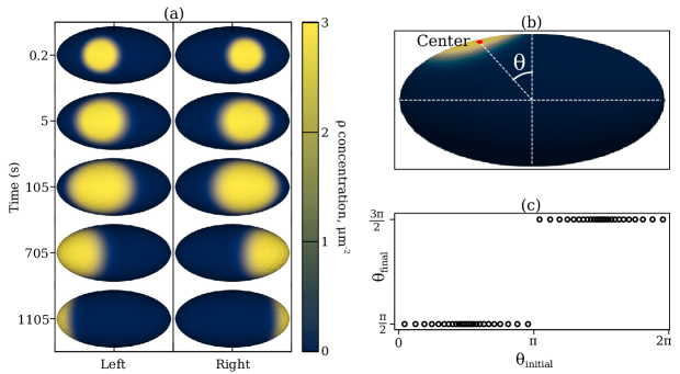
One of the motivating experimental results for this study is the reorientation of PAR protein domains in a C. elegans zygote Mittasch et al. (2018) to regions of high curvature. In these experiments, a C. elegans zygote of roughly ellipsoidal shape is subjected to cytoplasmic flows such that the high partitioning-defective protein (PAR) concentration domain is rotated from the initial position on one end of the zygote. If the induced rotation is less than 90^∘, the PAR domain goes back to its initial position. But for rotations greater than 90^∘ the polarity of the cell is reversed. Thus, in the steady state, the PAR domain is always on one of the ends of the long axis of the zygote. PAR proteins have reaction kinetics similar to the Rho GTPases i.e. there are membrane-bound active and cytosolic inactive forms that exchange Hoege and Hyman (2013), and PAR models have been built from extending WP models Goehring et al. (2011b). Therefore, the WP model may be an effective minimal model for some elements of PAR polarity. We test if the WP model can reproduce this bistability. We solve the reaction-diffusion system on an ellipsoidal surface, with initial conditions describing a high-$\rho$ domain at different angles $\theta$ (Fig. 2b). The WP model is able to reproduce the shape sensing behavior of PAR proteins. Figure  2a shows the top view of the ellipsoid as domains initialized close to $\theta=0$ (Fig. 2b) evolve over time. These domains move from the ellipsoid center towards its narrow ends over a duration of 18 minutes. A domain created just left of the center evolves to the left end, and a domain just right of the center evolves to the right end. We formalize this by tracking the angular position of the center of the high-$\rho$ domain (Fig. 2b). Varying the initial angular position, we find that domains initialized closer to the left end, i.e. $\theta_{\textrm{initial}}\in[0,\pi)$ end up at the left end ($\theta_{\textrm{final}}=\pi/2$), and all domains initialized closer to the right end, $\theta_{\textrm{initial}}\in(\pi,2\pi]$ have $\theta_{\textrm{final}}=3\pi/2$ (Fig. 2c). This is precisely the binary shape sensing observed by Mittasch et al. (2018). We emphasize that our model is not a full model of the PAR system, which should include the effect of antagonistic interactions between different PAR proteins and hydrodynamic flow Goehring et al. (2011b); however, it illustrates that minimalistic cell polarity models can capture binary shape sensing without additional assumptions. The time taken to reach the steady state decreases from 1800 s for $\theta$ near 0 to 100 s for $\theta$ near $\pi/2$, and naturally increases symmetrically as $\theta$ ranges from $\pi/2$ to $\pi$. This emphasizes the role of the initial condition’s symmetry: near-symmetric initial conditions can take a long time for a spontaneous symmetry breaking to occur.

Figure 3: Steady state shape of a domain on a smooth sinusoidal test surface. (a) Steady-state solution of the reaction-diffusion equations on a sinusoidal surface. Magenta lines are shown to illustrate the boundaries of the high-$\rho$ domain marked at $\rho=\left(\rho_{\textrm{max}}+\rho_{\textrm{min}}\right)/2$. (b) Steady state of reaction-diffusion model (color map, viewed from above), is in agreement with the perimeter minimization (solid magenta line).

II.2 Wave-pinning and perimeter-minimization agree on a simple smooth surface test problem

Figure 4: Domains on smooth surface robustly find peaks and valleys, with agreement between wave-pinning and perimeter minimization. (a) Rendering of the surface in Eq. 6. (b) and (c) show the trajectories and steady-state positions of domains in the WP and PM models respectively. In both, the uniformly spaced grid of small blue dots indicate the initial position of a domain, the white line indicates the domain’s trajectory, and heavy red dots are the domain’s final location. Color maps are contours of the height $h(x,y)$.

To understand how the dynamics of wave-pinning depend on membrane shape in a simple context, we begin with a sinusoidal surface (Fig. 3a)

$$h(x,y)=h_{0}\sin{\frac{2\pi x}{W_{0}}}\cos{\frac{2\pi y}{W_{0}}}$$ (6)

where $h_{0}=5.55\,\muup\textrm{m}$ and $W_{0}=20\,\muup\textrm{m}$, and the system spans $-W_{0}/2\leq x,y\leq W_{0}/2$. The surface represents a portion of the cell membrane, and its size and curvature are similar to that of the ellipsoid. This surface has the advantage of being able to be represented as a function $z=h(x,y)$, making perimeter minimization simpler (see Appendix for numerical methods).

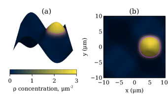
We solve the reaction-diffusion equation Eq. 1 on the simple sinusoidal surface. We find that, initializing the system with a region of high $\rho$ concentration near one of the surface peaks, the high-activity domain migrates to the peak at long times (Fig. 3a, Movie 1). We simulate the reaction-diffusion process for 5,000 seconds to ensure we have converged to the steady state, but all but a few domains reach a steady state within a few hundred seconds (see, e.g. Movie 1). The WP model gives as a result a concentration $\rho$ on the surface that decreases rapidly but smoothly from a maximum value $\rho_{\textrm{max}}\approx\rho_{+}$ to a minimum value $\rho_{\textrm{min}}\approx\rho_{-}$. To define an explicit domain shape and size as in the perimeter minimization, we must choose a threshold. We choose the contour of $\rho=\frac{1}{2}\left(\rho_{\textrm{min}}+\rho_{\textrm{max}}\right)$ as the boundary for calculating the area and shape of the high $\rho$ concentration domain. Fig. 3b shows the “top” view of the sinusoidal surface of Fig. 3a. The curve in magenta indicates the steady-state shape of the domain obtained from perimeter minimization (Eq. 5), which agrees closely with the transition from high to low $\rho$. This is consistent with our idea that perimeter minimization is a good heuristic for explaining the shape-sensing behavior.

Steady-state location of high activity domain depends on domain initial position

Figure 5: Surface roughness disrupts shape-sensing as shown by the presence of steady states at locations away from the global peaks and the valleys of the surface. The wave-pinning model is more robust to it than perimeter minimization predicts as it has fewer such local steady states. (a) Rendering of the surface in Eq. 7 with $h_{1}$ as 10% of $h_{0}$. (b) and (c) show the steady-state positions and the trajectories obtained from WP model and PM model respectively for the surface in Fig. 5a. (d) Rendering of the surface in Eq. 7 with $h_{1}$ as 20% of $h_{0}$. (e) and (f) show the steady-state positions and the trajectories obtained from WP model and PM model respectively for the surface in Fig. 5d. As in Fig. 4, the uniformly spaced grid of small blue dots are domain initial positions, white lines are domain trajectories, and heavy red points are domain final positions. Colors indicate contours of $h(x,y)$.

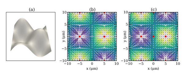
Our results in Fig. 2 and the experimental results of Mittasch et al. (2018) show that regions of high active polarity protein concentration on the membrane will evolve to different steady-state locations depending on their initial location. What trajectory do they take? Our simple test surface $h(x,y)$ has multiple peaks and troughs as potential steady-state locations for domains. To understand how domains choose their steady-state positions and what trajectory they take, we simulate domains starting from 625 initial positions shown as a small grid of blue dots in Fig. 4. We do these simulations in both the wave-pinning and perimeter minimization models. The big red dots indicate the steady state position of the center of mass of the domains. A thin white line connecting a blue dot with a red dot indicates the trajectory of the center of mass of the domain. Generally, we observe that a domain migrates to the peak or valley that is closest to it (Fig. 4). Interestingly, for points that are initialized nearly equidistant between two peaks or valleys, these domains follow a trajectory tracing out the line of symmetry between these points. The PM model and the WP model are in very good agreement in both their predicted trajectories and steady-state domain locations. While earlier work has suggested that WP models have a perimeter-minimizing property Jilkine (2009); Marée et al. (2012); Vanderlei et al. (2011), it is somewhat surprising that the trajectories match this well between the PM and WP model, given the simplified overdamped dynamics we have chosen.

There is a small disagreement between PM and WP for the three red dots along the central vertical line in the minimization plot of Fig. 4. From the perspective of the energy minimization, peaks and troughs of the sinusoid are equivalent. Therefore, the central vertical line is a line of symmetry. Domains that start with their center of mass exactly equidistant from a peak and a trough don’t migrate in the PM model, but do in the WP model, where the symmetry is broken at a shorter timescale. The exact timescale of breaking a symmetry like this will depend on both the details of the initialization and the rate of accumulation of floating point errors in both models. Therefore, we would not necessarily expect these domains initialized precisely on lines of symmetry to agree between WP and PM. We argue that the apparent steady-states (red dots) away from the peaks and valleys in Fig. 4 in the PM model are long-lived transients. Small perturbations away from these apparent steady states leads to the domains migrating to the peaks and valleys, as with the other domains (Fig. S1).

II.3 Shape sensing is disrupted on rough surfaces

Cell membranes have roughness due to the presence of filopodia, blebs, embedded proteins, etc. Any mechanism for domain localization should be robust to this roughness. Therefore, we would like to check if our models are robust in predicting the steady states for rough surfaces. How rough can a surface be before shape sensing by WP or PM breaks down? We characterize the disruption of shape sensing by determining whether domains initialized to different locations on the membrane can still migrate to the global peaks and valleys when additional roughness is introduced. To answer this question we superimpose a small wavelength roughness of increasing amplitude on the smooth sinusoidal surface,

$$h(x,y)=h_{0}\sin{\frac{2\pi x}{W_{0}}}\cos{\frac{2\pi y}{W_{0}}}+h_{1}\sin{\frac{2\pi x}{W_{1}}}\cos{\frac{2\pi y}{W_{1}}}$$ (7)

where $W_{1}=4\,\muup\textrm{m}$ and we choose the amplitude of the perturbation $h_{1}$ to be 10% or 20% of the amplitude $h_{0}$.

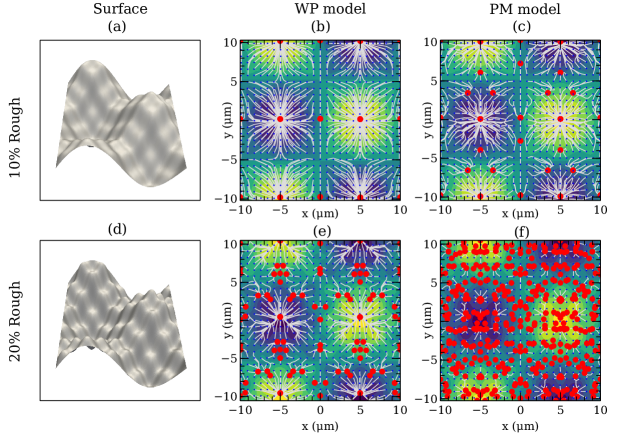
We analyze the steady state positions of domains for the same set of starting positions as studied in Fig. 4. These results are somewhat involved, and are presented in Figs. 5–7.

Domain steady-states and trajectories

How are the domain steady states and trajectories altered in the presence of roughness? Fig. 5b shows how domains move in the WP model for a surface with 10% roughness ($h_{1}=0.1h_{0}$), showing steady states as red dots. Most of the steady states are the same as in Fig. 4 except for the three red dots at $x=-5\ \mu\mathrm{m}$ and the three red dots at $x=5\ \mu\mathrm{m}$, which lie along lines of symmetry and can be long-lived transients as discussed above. We find then that the WP model still localizes domains to the peaks and valleys in the presence of a roughness of 10% amplitude of the smooth surface.

Fig. 5e shows the steady states of the WP model for the 625 initial conditions for the surface with roughness 20%. Now we see several new steady states emerge in addition to the steady states of the smooth surface. Again, we have some clusters of steady state around the lines of symmetry at $x=\pm 5\ \mu\mathrm{m}$ but there are other steady states which are not near any lines of symmetry. Thus, the shape-sensing ability of the WP model – in the sense of its ability to find the global peaks and valleys – has deteriorated for the increased roughness.

Figure 6: Steady-state domain shapes agree between wave-pinning and perimeter minimization even at 20% roughness. Three representative examples are shown from the subset of initial conditions where steady-state centroids are in agreement between WP and PM (see text).

On a smooth surface, a domain that minimizes perimeter while keeping area fixed localizes robustly to the peaks and valleys of the surface and also reproduces the evolution of the WP model (Fig. 4). Both of these properties fail for a sufficiently rough surface. Fig. 5c shows the solution of the PM model for the 10% surface roughness. In comparison with Fig. 4 we note the emergence of extra steady states, including states that are not near the lines of symmetry and cannot be discounted as very long-lived transients. We argue that the shape-sensing ability of the PM model is affected more than the WP model for the same amount of surface roughness.

More dramatically, solving the PM model on a surface with 20% roughness shows a huge increase in the number of steady states (Fig. 5f) – domains do not typically move over any significant distance on the surface and are largely localized to near their initial position. The ability of the PM model to find global peaks and valleys has broken down. As we noted above, in the WP model, domains do not perfectly localize to the troughs and peaks at 20% roughness, but the level of new steady states created in PM at 20% roughness is qualitatively worse. This, again, suggests the relative robustness of the WP model.

Domain Shapes

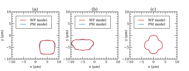
For smooth surfaces, the steady states, trajectories, and shapes of domains are identical between the perimeter minimization and wave-pinning models (Fig. 3b, 4). In the presence of surface roughness, though, the steady states and trajectories do not match between WP and PM (Fig. 5). Does this indicate a complete failure of the matching between the PM model and the WP model, or worse – was the match we saw in Fig. 4 a coincidence? To check this question, we test if the PM model and WP model can reproduce the same steady-state domain shapes. However, it is only appropriate to compare the domain shapes at the same location on the surface $h(x,y)$. For the 20% roughness case, the number of steady states predicted by the PM model (Fig. 5f) is much larger than the number of steady states predicted by the WP model (Fig. 5e), but for some of the 625 initial conditions, the steady states of the WP model and the PM model have centroids that are close to each other. We compare domain shapes between PM and WP when the predicted steady-state domain centroids are in agreement (within a tolerance of 0.15 $\mu\mathrm{m}$), finding that domain shapes match well between the models even in the presence of 20% surface roughness (Examples shown in Figs. 6a, 6b, 6c). These shapes are nontrivial and complex, very different from the circular domains found on the smooth surface, and the agreement is excellent. Even though the PM model is unable to give the same trajectories and the same steady states as the WP model, it is still quite robust at reproducing the domain shapes.

Figure 7: Steady states predicted by perimeter minimization are sensitive to domain size. We have highlighted the steady states at the peak, marked with white squares, which is markedly different in the three subfigures. (a), (b), and (c) show the steady state positions and the trajectories given by the PM model when the domain area is set to 8%, 9%, and 10% of the total surface area respectively. As in Fig. 4, the uniformly spaced grid of small blue dots are domain initial positions, white lines are domain trajectories, and heavy red points are domain final positions. Colors are the contour map of $h(x,y)$.

II.4 Perimeter minimization on rough surfaces is fragile to small changes in domain area

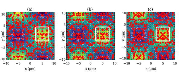
We saw in the previous section that perimeter minimization can predict complex nontrivial domain shapes that appear in the WP model (Fig. 6). This suggests that the steady states of WP do obey a perimeter minimization principle – at least locally. However, the large-scale trajectories and many of the steady states differ between the PM model and the WP model. Why? The PM model has a tight constraint on the domain area, while in the WP model the domain area is only approximately fixed. In fact, for the WP model the domain area varies slightly for different starting positions of the center of mass and also at different locations of the center of mass along the trajectory. For the simulations shown in Fig. 5, we found that the domain area ranged from 8%-10% of the total surface area of the rough membrane. Does perimeter minimization predict the same domain steady state location or trajectory for these different values of domain area? Figures 7a-c show the trajectory plots obtained from the PM model when domain area is constrained to a value $A_{0}$ that is 8%, 9%, and 10% of the total surface area for the surface with 20% roughness. The local minima predicted for different domain areas are different (see, e.g. white boxes in Fig. 7a-c). This shows that strict perimeter minimization on a rough surface is fragile – it depends so strongly on the target area $A_{0}$ that we should not expect agreement between WP and PM.

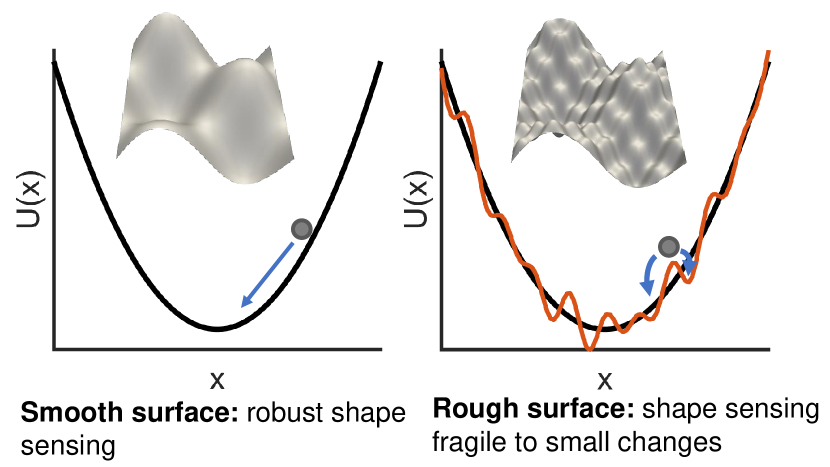
The fragility of perimeter minimization to small changes in area can be understood by thinking about the domain as moving within an effective energy landscape $U(x)$ (Fig. 8). When the surface $h(x,y)$ is smooth, this landscape is also smooth, and a domain can smoothly travel to the peak or trough – the energy minimum. However, when the surface becomes rough, we expect the effective energy landscape to also become rough (Fig. 8, right) – and domains become trapped in local minima. More importantly for this section, we can see that small perturbations to the landscape – as might be expected from changing the domain area – can lead to large shifts in the steady state. This corresponds with the fragility observed in Fig. 7.

Figure 8: Movement of the domain over a surface is like moving a particle through energy landscape $U(x)$; shape-sensing is like finding the minimum energy position. For a smooth surface, the global minimum is easily attained but for rough surfaces there are local minima with energy barriers that prevent reaching the global minimum. Small changes to initial condition or the landscape parameters lead to changes in outcome (blue arrows, right)

II.5 How reaction-diffusion shape sensing can be made robust to membrane roughness

The sensitivity of the PM model to the domain area does not fully explain the difference between the steady states shown in Fig. 5 – the WP model has many fewer unique steady-states than any of the PM results presented in Fig. 7. Why is the WP model so robust?

Effect of diffusion coefficient

The high $\rho$ concentration domain formed by wave-pinning has a finite interface width as shown in Fig. 3a. The PM model domain, on the other hand, has a sharp interface. The width of the interface increases with the diffusion coefficient of the reaction-diffusion system Hubatsch et al. (2019). So as we decrease the diffusion coefficient, the interface width of the WP model will decrease – potentially leading to better agreement between WP and PM.

For the smooth surface, the WP model and the PM model are in good agreement (see Fig. 4), and reducing the diffusion coefficient in the WP model does not alter the results for this surface (Fig. 9a,d).

Figure 9: In the WP model, the width of the interface of high activity domain can be decreased by reducing the diffusivity. As the WP model approaches the sharp interface limit, many local minima steady states appear. (a), (b), and (c) show the steady state positions for $D=0.5\mathrm{\mu m^{2}s^{-1}}$ for increasing surface roughness. (d), (e), and (f) show the corresponding steady state positions for $D=0.1\mathrm{\mu m^{2}s^{-1}}$ for increasing surface roughness. As in Fig. 4, the uniformly spaced grid of small blue dots are domain initial positions, white lines are domain trajectories, and heavy red points are domain final positions. Colors are contour map of $h(x,y)$.

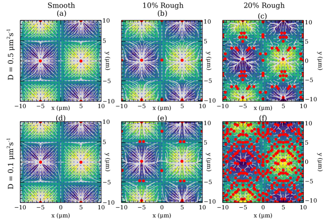
In our default parameters, domains in the WP model largely reach the peaks or valleys of the surface at 10% roughness (Fig. 5b). However, on reducing the diffusion coefficient from $0.5\ \mu\mathrm{m\,s}^{-1}$ to $0.1\ \mu\mathrm{m\,s}^{-1}$, the WP model begins to show nontrivial local minima (Fig. 9e), albeit different from those shown by the PM model as shown in Fig. 5. As we increase the surface roughness to 20% for $D=0.1\ \mu\mathrm{m\,s}^{-1}$, the number of local minima for the smaller diffusion coefficient increases significantly (Fig. 9f). The number of local minima for $D=0.1\ \mu\mathrm{m\,s}^{-1}$ for the 20% roughness case are comparable to the number of local minima seen in the PM model (see Fig. 5f).

We emphasize that our results in Fig. 9 show that decreasing the diffusion coefficient increases the number of steady states – this is not just an artifact of decreasing diffusion making kinetics slower. Because of the slower diffusion coefficient, we ran the simulations in Fig. 9 with $D=0.1\mu m^{2}/s$ for a time of $20000$ s, compared with $5000$ s for $D=0.5\mu m^{2}/s$. We also ensured that these steady states were converged by running the simulations for finer finite element meshes, and for longer simulation times for a subset of the initial positions.

We argue that the robustness of the WP model as compared to the PM model is due to the finite interface width of the high $\rho$ concentration domain, and that we can control whether the WP model seeks the true peaks and valleys or gets stuck in local minima in part by changing this interface width via $D$.

Effect of domain size

Along with size of the roughness, and the size of the interface, the diameter of the high $\rho$ concentration domain is another length scale in this problem. Can cells sense shape more effectively when the domain is probing a larger length scale? We investigate the effect of size of the high $\rho$ concentration domains on the steady states by increasing $M/S$, which strongly influences domain size, from $2.9\ \mu\mathrm{m}^{-2}$ to $3.2\ \mu\mathrm{m}^{-2}$. This increases the typical domain size to $\sim$18% of the surface.

Figure 10: Increasing the size of high activity domains enhances the shape-sensing ability of the WP model. The steady state positions in (b) are closer to the global peaks and valleys. (a) shows the steady states and trajectories obtained from the WP model when $M/S=2.9\mu m^{-2}$ and the size of the domains is 9% of the total surface area. (b) shows the steady states and trajectories obtained from the WP model when $M/S=3.2\mu m^{-2}$ and the size of the domains is 18% of the total surface area. As in Fig. 4, the uniformly spaced grid of small blue dots are domain initial positions, white lines are domain trajectories, and heavy red points are domain final positions. Colors are a contour map of $h(x,y)$.

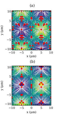
For the smooth surface and the surface with 10% roughness, there were no local minima in the WP model (see Fig. 4) and Fig. 5b). Increasing the domain size did not produce any significant difference in these two cases. But for the surface with 20% roughness, some of the local minima that were not situated on any line of symmetry appear to “coalesce” as shown in Fig. 10. At the lines of symmetry, as we have already noted, it is difficult for the domains to localize to a unique solution. So, in general, it seems that increasing the domain size, increases the robustness of the shape-sensing slightly.

II.6 Shape sensing occurs in a broad range of biologically-relevant geometries

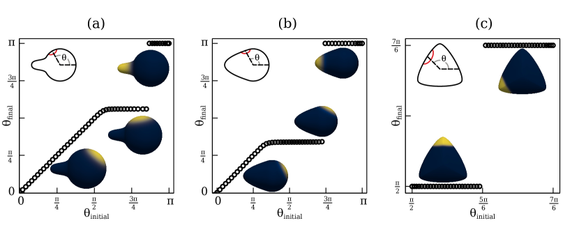
The insight we have developed in the simple sinusoidal surface can help us understand both past computational work and experiments beyond our motivating example of binary shape sensing Mittasch et al. (2018). We show the evolution of the wave-pinning reaction-diffusion model on three different 3D surfaces in Fig. 11: a sphere with a bump and a sphere with a larger bump, both approximating the shmoo-like structures of mating yeast as previously simulated in, e.g. Orlandini et al. (2013); Trogdon et al. (2018), and a cell with triangular symmetry. This last shape models C. elegans zygotes studied in triangular confinement by Klinkert et al. (2019). We have argued above that, on smooth surfaces at least, the high-activity domain evolves to locally minimize the perimeter while keeping a fixed area. What would perimeter minimization predict on these surfaces? Let us think about a perfect sphere first. Given the rotational symmetry of a sphere, no angle is preferred, so a domain initialized in one location will stay in that location, as if it were on a flat surface. Similarly, because the sphere with a bump is locally identical to a sphere, except in the immediate vicinity of the bump, we expect domains to remain at their initial centers of mass. We then simulate the wave-pinning equations for a sphere with a bump in Fig. 11a. When we initialize domains at different angles with respect to the bump, we find that domains on the larger spherical region remain at their initial angle. However, when domains are initialized closer to the bump, they are repelled by the bump – localizing to the nearest undistorted portion of the sphere. This is similar to the final localization observed in Orlandini et al. (2013) in a similar geometry (Fig. 7A in that paper). However, once the domain is initialized sufficiently close to the bump, it localizes to a final position on the bump – the local minimum of perimeter with fixed area. This “sphere with a bump” geometry is particularly informative because it has a large region that is identical to an unperturbed sphere – leading to a large fraction of the surface where domains will not migrate significantly. This shows the value of understanding the dynamics in terms of a local minimization of perimeter: even though there is a “global” location with smaller perimeter – placing the domain at the bump – domains initialized on the sphere do not migrate. This may explain why shape sensing in related reaction-diffusion models was viewed as weak Orlandini et al. (2013). By contrast, if the region of the bump is increased (Fig. 11b), domains become attracted to the peak over a larger range of initial conditions. These results show how shape sensing can be disguised on surfaces that are sufficiently close to a sphere. Our results also illustrate that it is essential to study a range of different initial conditions: there are often many different steady states even on a simple surface, and a full understanding of shape sensing requires seeing under which conditions different initial conditions converge to these steady states.

More excitingly, we see that the same mechanism of shape sensing by wave-pinning that we have studied above can explain additional elements of domain localization. In Fig. 11c, we simulate the wave-pinning reaction-diffusion model on a cell with triangular symmetry, similar to the shapes of zygotes confined in triangular wells studied by Klinkert et al. (2019). In that paper, the authors found that in zygotes depleted of AIR-1, PAR-2 localized to the triangular corners of the cell – the regions of high curvature – and were able to reproduce this with a model in which the rate of binding to the membrane was sensitive to curvature. Here, we show that curvature-dependent binding is not necessary to reproduce localization to the corners. If we initialize a domain to the sides of the cell, we observe that it migrates to the corner (Fig. 11c). This is, again, consistent with our intuition from the perimeter minimization idea: domains with the same area will have a lower perimeter if they are localized to the tips. (We note: for the corners to have a lower perimeter, there must be some Gaussian curvature at the corners of the cell. We would not expect corner localization if the cell were shaped, for instance, like a triangular prism.) Corner localization behavior would not have been seen in the original simulations of Klinkert et al. (2019) in the absence of curvature-dependent binding rates $k_{\textrm{on}}$, because they worked in one dimension – which does not resolve the full shape of the domain’s perimeter. While the wave-pinning model does not serve as a complete model for the PAR system, it shows that a minimalistic cell polarity mechanism can reproduce corner localization without any additional assumptions.

Figure 11: Shape sensing from wave-pinning occurs in a broad range of biologically-relevant three-dimensional cell shapes. We show the final angular position of a domain as a function of its initial angle, as in Fig. 2c. $\rho$ concentration is plotted for representative examples. Cell shapes are a) spheres with a bump (“shmoo”), b) teardrop, and c) a samosa shape modeling a cell in a triangular confinement Klinkert et al. (2019). Domains initialized at one location on a three-dimensional cell surface systematically evolve to their nearest steady-state location.

III Discussion

In this paper, we have shown that the classic wave-pinning model of cell polarity is sufficient to produce the behavior of binary shape sensing observed by Mittasch et al. (2018) – as might be anticipated by earlier work Camley et al. (2017); Cusseddu et al. (2019); Vanderlei et al. (2011). We then try to capture some of the essential features and limitations of shape sensing by the wave-pinning Rho GTPase dynamics as well as developing a heuristic model for it in terms of minimization of an effective energy proportional to the domain perimeter. Wave-pinning reliably senses cell shapes when the cell is smooth, but introduction of surface roughness significantly disrupts this process. The ability of wave-pinning to sense cell shape in the presence of roughness is controlled by both the diffusion coefficient $D$ on the surface (Fig. 9) and the domain size (Fig. 10). The perimeter minimization heuristic captures much of the dynamics of domain migration, but fails on rougher surfaces (Fig. 5) due to the relevance of finite interface sizes and domain area fluctuations (Fig. 7). However, the perimeter minimization heuristic does let us understand when domains on more complex, biological shapes should migrate, including predicting the corner-localization of PAR domains in triangular confinement (Fig. 11.

How fast is shape sensing by wave pinning? Does it occur on a biologically relevant timescale? In the experiments on long-axis polarization of PAR proteinsMittasch et al. (2018), the high-PAR concentration domain reaches a steady states in approximately 10 minutes. Our modeling shows that protein domains attain their steady states on a timescale of 100-1800 seconds, compatible with a roughly 10 minute timescale. The longest times required to reach steady state occur when the domain is initialized nearly symmetrically, requiring a symmetry breaking. The timescale is similar between the three-dimensional ellipsoidal domain and our smooth sinusoidal surfaces, where except for those initial conditions at lines of symmetry, domains take $\sim$ 100-500 s to reach steady state. Earlier work from Cusseddu et al. have reported results for WP simulations on a capsule Cusseddu et al. (2019), similar to the ellipsoidal shape of Section IIII.1, finding a much longer time of 13463 s to reach steady state. This may have been influenced by a symmetric initial condition. However, unlike their simulation model, we have assumed that the interior is well-mixed, and we have also chosen a larger diffusion coefficient of 0.5 $\mu$m²s^-1 compared to their value of 0.1 $\mu$m²s^-1. Koo et al Koo et al. (2015) have reported in vivo experimental results that Rho GTPases show six different diffusive states of which the average diffusivity of the most probable diffusive states is closer to $0.5$$\mu$m²s^-1, though we note that our model does not yet address the possibility of multiple states with different diffusion coefficients. The diffusion coefficients and kinetics may influence the plausibility of shape sensing in different contexts. If the time to attain the steady state is as long as 13000 seconds, the large-scale shape of the cell will likely change due to other phenomena, like formation of protrusions, before shape-sensing by wave-pinning happens. Earlier work finding relatively weak effects of membrane shape on polarization Orlandini et al. (2013) used membrane diffusion coefficients based on those for yeast, $D\approx 0.0025\mu m^{2}/s$ Goryachev and Pokhilko (2008); this value is orders of magnitude smaller than in our case, and may lead to very slow, if any, shape sensing. Future work incorporating reaction-diffusion on a moving membrane (following, e.g. Tamemoto and Noguchi (2020, 2021)) would be required to understand whether shape sensing that is slow relative to surface motion would probe the time-averaged surface or be disrupted by dynamic changes.

Our results show that, at least for smooth surfaces, the reaction-diffusion WP model is well-captured by perimeter minimization. This result is consistent with earlier work relating mass-conserved reaction diffusion equations and coarsening driven by interfacial tension (i.e. perimeter minimization) in simpler contexts Tateno and Ishihara (2021); Bergmann et al. (2018); Brauns et al. (2020), as well as the analysis of Jilkine (2009). However, our work highlights crucial limitations of these assumptions. The fragility of energy minimization on rough surfaces to small changes in area (Fig. 7) shows that an approximate conservation of domain area is not sufficient to completely characterize domain trajectories and steady states, and that the full reaction-diffusion equations need to be solved. In addition, we note that the WP model consists of two stable phases only when the concentration of the inactive form is in a suitable range Mori et al. (2008); Cusseddu et al. (2019). The ability of cells to sense shape, as with their ability to polarize Hubatsch et al. (2019), will be dependent on cell size and total Rho GTPase amount.

Throughout this paper, we have assumed that the cytosolic component of the Rho GTPase is well-mixed and therefore uniform. This contrasts with the key role of the cytosolic diffusion proposed in long axis selection by Geßele et al. (2020), and the full bulk-surface implementation of the wave-pinning model in Cusseddu et al. (2019). The well-mixed cytosol is a common assumption, given the large difference in cytosolic and membrane-bound diffusion coefficients, but it is a potential limitation of the model. If we extended our model to allow for a finite level of cytosolic diffusion, the cytosolic inactive form might not be homogeneous, as observed previously Marée et al. (2012). With an inhomogeneous cytosol, the local ratio of surface area to volume might play a significant role Meyers et al. (2006). This would break the symmetry in our model between positive and negative curvature – peaks and valleys would no longer be identical from the point of view of the model.

Our approach shows that shape sensing may emerge from wave pinning without any explicit dependence upon membrane curvature in protein binding or kinetics. Previous work has suggested that in order to explain PAR domain localization in C. elegans zygotes in triangular confinement, binding rates in the reaction-diffusion model must be dependent on curvature Klinkert et al. (2019). We have shown in Fig. 11 that the corner localization of these domains does not require this curvature-dependent binding, but can be reproduced solely from the minimal reaction-diffusion wave pinning model if simulated in a three-dimensional geometry. If we extended our model to study explicit dependence of binding rates on local curvature, this dependence could also be used to break the symmetry between positive and negative curvature, as with cytosolic diffusion. However, the ability of single proteins to sense micron-scale curvature on their own is rare, and many aspects of the mechanism of micron-scale curvature sensing remain unresolved Cannon et al. (2017, 2019). We are not aware of any evidence showing that Rho GTPases or PAR proteins have binding rates that depend on local curvature. We therefore suggest that preferences for different signs of curvature are more likely to arise from cytosolic diffusion effects.

Our results show that surface roughness can impede shape sensing by both energy minimization and Rho GTPase dynamics, with perimeter minimization more strongly affected. How crucial is the effect of roughness to understanding shape sensing in realistic geometries? This likely varies between cell types: the C. elegans zygote appears fairly smooth on the micron scale Mittasch et al. (2018), while at the other extreme, blebby cell surfaces may have overhangs and extremely complex involutions Driscoll et al. (2019), for which the mechanism of domain migration shape sensing studied here seems implausible. The importance of roughness is also dependent on the diffusivity of the membrane-bound Rho GTPases (Fig. 9). Diffusion of polarity proteins could be altered by their coupling to the cytoskeleton or other proteins Gowrishankar et al. (2012); Kusumi et al. (2011); Hosaka et al. (2017); Swartz and Camley (2021), controlling the extent to which shape sensing leads to domains finding the global peaks and valleys or long axis, or rather becoming pinned to a local minimum. It is also possible to regulate the size of polarity domains by changing the available concentration of Rho GTPases; this will also alter shape sensing (Fig. 10).

Our results clarify both the power and limits of shape sensing by reaction-diffusion and perimeter minimization: in the best case, shape sensing proceeds in a straightforward, predictable way, and robustly finds the minima and maxima in reasonable amounts of time. However, both mechanisms are fragile to sufficiently rough perturbations. This suggests that many past models of spontaneous cell turning, cell polarization, etc., Camley et al. (2017); Goehring et al. (2011a); Edelstein-Keshet et al. (2013); Mogilner et al. (2012); Holmes et al. (2017) may need to be systematically tested to determine to what extent they are robust to realistic changes in cell geometry.

Code availability

Simulation code for reaction-diffusion and perimeter minimization is posted on Zenodo: https://zenodo.org/record/6731244

SI Appendix

Appendix A Movie captions

Movie 1: Evolution of wave-pinning model on the sinusoidal surface showing the migration of a domain from its initial position to the final position at the surface peak. View is from the top.

Appendix B Parameter Values

We tabulate the default parameter values used in our simulations. Any changes from the default values have been explicitly mentioned in the main text.

Parameter	Default Value	Description
$k_{0}$	0.07 $\mathrm{s}^{-1}$	Basal activation rate
$\gamma$	5 $\mathrm{s}^{-1}$	Positive feedback activation rate
$K$	2 $\mu\mathrm{m}^{-2}$	Saturation parameter
$\delta$	3 $\mathrm{s}^{-1}$	Deactivation rate
$D$	0.5 $\mu\mathrm{m}^{-2}\mathrm{s}^{-1}$	Diffusion coefficient of the active $\rho$
$M/S$	2.9 $\mu\mathrm{m}^{-2}$	Total concentration (see Eq. 3)
$S_{R0}$	627 $\mu\mathrm{m}^{2}$	Total surface area of the smooth surface
$S_{R10}$	664 $\mu\mathrm{m}^{2}$	Total surface area of the surface with 10% roughness
$S_{R20}$	768 $\mu\mathrm{m}^{2}$	Total surface area of the surface with 20% roughness
$A_{R0}$	0.09 $S_{R0}$	Surface area constraint for PM model on the smooth surface
$A_{R10}$	0.09 $S_{R10}$	Surface area constraint for PM model on the 10% roughness surface
$A_{R20}$	0.09 $S_{R20}$	Surface area constraint for PM model on the 20% roughness surface
$k$	$10^{3}\ \mu\mathrm{m}^{-1}$	Penalty coefficient (see Eq. 4)
$\beta$	$10^{-2}\ \mu\mathrm{m}$	Gradient-descent step size coefficient (see Eq. 5)
$T_{\textrm{sim}}$	5,000 s	Simulation time ($D=0.5\mu m^{2}/s$ simulations)
$N_{\textrm{elem}}$	80000	Number of mesh elements

Table S1: Default values of the parameters used in the simulations of the PM and the WP models.

Appendix C Transient States in Perimeter Minimization

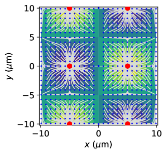
In Fig. 4c, we noted that perimeter minimization predicts some three “steady” state along the $x=0$ line that have been marked as red dots in the plot. The initial positions of the centroid of the domains in all of these cases were along the $x=0$ line which is a line of symmetry. If we apply a small random perturbation of 0.02 $\mu$m to each point $(x_{i},y_{i})$ of the final states of these simulations, they attain steady states on one of the peak or valleys. Thus, we confirm that these are indeed transient states and are an artefact of the symmetry of the surface. Fig. S1 show the trajectory plot after perturbing the final states.

Figure S1: The steady states and trajectories obtained from the perimeter minimization simulations on the smooth surface after applying a small perturbation to the final states along $x=0$ line shown in Fig. 4.

Appendix D Details of the Numerical Methods

D.1 Finite Element Model for Wave-pinning on a 3D surface

Our approach uses some standard finite element tools: this section will be easier to follow with knowledge of weak forms of PDEs, discretization of the domain of PDEs into a linear triangular mesh, the shape functions of a linear triangular element, and Gaussian quadrature on linear triangles to evaluate integrals defined over the elements.

We want to solve the following system of equations

$$\partialderivative{a}{t} =D\laplacian a+f(a,b)$$

$$b =\alpha-\frac{1}{S}\int_{\Omega}a$$

using the Finite Element Method. Here, for conciseness, we’ve written the membrane-bound concentration as $a$ and the uniform cytosolic concentration as $b$. $\alpha=\frac{M}{\omega S}$. We’ve also implicitly assumed $\omega=1\mu m$ here, but this can be generalized to nonzero $\omega$ by taking $S\to\omega S$ in the final equations. The first step for setting up the finite-element problem is to derive the “weak form” of the PDEs. We can express the time derivative using finite-difference. Let $a$ be the concentration at time-step $n$ and $\bar{a}$, be the value of $a$ at time step $n-1$. Let the time step size be $t$.

$$a-\bar{a}=tD\laplacian a+tf(a,b)$$

We will linearize the non-linear reaction function $f(a,b)$ using $a^{k+1}=a^{k}+\delta a$ and $b^{k+1}=b^{k}+\delta b$. Here $\delta a$ is the correction to the value of $a^{k}$ at the $k$th Newton iteration and similarly for $\delta b$.

$$a^{k+1}-\bar{a} =tD\laplacian a^{k+1}+tf(a^{k+1},b^{k+1})$$

$$a^{k}+\delta a-\bar{a} =tD\laplacian a^{k}+tD\laplacian\delta a+tf(a^{k},b^{k})+tf_{a}(a^{k},b^{k})\delta a+tf_{b}(a^{k},b^{k})\delta b$$

where $f_{a}$, and $f_{b}$ are the derivatives of $f$ with respect to $a$ and $b$ respectively. Collecting the terms in $\delta a$ and $\delta b$ on the LHS,

$$\left(1-tf_{a}(a^{k},b^{k})\right)\delta a-tD\laplacian\delta a-tf_{b}(a^{k},b^{k})\delta b =\bar{a}-a^{k}+tD\laplacian a^{k}+tf(a^{k},b^{k})$$

Multiply both sides by $u$, the test function, and integrate by parts setting the boundary terms to zero due to the boundary conditions (which will be either no flux or periodic).

$$\int_{\Omega}\left(1-tf_{a}(a^{k},b^{k})\right)u\delta a\differential{\Omega}+tD\int_{\Omega}\gradient u\cdot\gradient\delta a\differential{\Omega}-t\int_{\Omega}f_{b}(a^{k},b^{k})u\delta b\differential{\Omega}=$$ (8)

$$\int_{\Omega}u(\bar{a}-a^{k})\differential{\Omega}-tD\int_{\Omega}{\gradient u\cdot\gradient a^{k}}\differential{\Omega}+t\int_{\Omega}uf(a^{k},b^{k})\differential{\Omega}$$

We will simplify the constraint equation using these linearizations, $a=a^{k+1}=a^{k}+\delta a$ and $b=b^{k+1}=b^{k}+\delta b$:

$$b^{k}+\delta b=\alpha-\frac{1}{S}\int_{\Omega}\left(a^{k}+\delta a\right)\differential{\Omega}$$

Collecting $\delta a$ and $\delta b$ on the LHS, we get

$$\left(\frac{1}{S}\int_{\Omega}\delta a\differential{\Omega}\right)+\delta b=\alpha-b^{k}-\frac{1}{S}\int_{\Omega}a^{k}\differential{\Omega}$$ (9)

The integral equations 8 and 9 are the weak forms of the original PDEs. Our goal is to solve for $\delta a$, and $\delta b$. But this is an infinite-dimensional problem because $\delta a$ varies continuously over the surface although $\delta b$ is uniform. FEM converts the infinite-dimensional problem to a finite-dimensional problem i.e. a system of equations. It does this by discretizing the domain of the system of PDEs into a discrete mesh of simple geometric entities called as the “finite elements” like triangles, or rectangles (or tetrahedrons and hexahedrons for higher-dimensional domains). In our problem, the domain $\Omega$ is a surface. The surface is discretized into a mesh of triangles $\Omega_{e}$ where $e=1,2,\ldots$. Fig. S2 shows a sample surface domain discretized into linear triangular elements.

Figure S2: A sample surface $\Omega$ which is the domain of a PDE to be solved using FEM is shown with its boundaries as bold lines. It has been discretized into a mesh of non-overlapping linear triangles $\Omega_{e}$ where $e=1,2,\ldots,8$ shown with thin lines. The circular dots are the nodes of the mesh that are coincident with the vertices of the triangles. The bold numbers show the global indices of the nodes. The italic numbers show the local indices of the nodes in a triangle. The number in parenthesis indexes the triangles.

The next step in FEM is to discretize all the field variables in all the integrands in the above equations into their values at the “nodes” of the finite element. Fig. S2 shows the nodes of a sample finite element mesh along with one possible way to index the nodes globally and locally. The number and location of nodes depends on the type of finite element being used. A node of the finite element mesh may be shared between multiple finite elements e.g. in Fig. S2 global node 1 is the same as local node 1 for triangle (1) and local node 3 for triangle (2). It is useful to define a mapping between the global and local indices of the nodes. Let $E$ be the total number of elements in the mesh, $G$ be the total number of nodes in the finite element mesh, and let $N$ denote the number of nodes per element. Let $I$ denote the global index of a node and $i^{(e)}$ denote its local index in the $e^{th}$ element. We can define a mapping between the global and local nodes

$$\Lambda^{(e)}:\{I\}_{I=1}^{I=G}\to\{i^{(e)}\}_{i=1}^{i=N}$$

or equivalently

$$i^{(e)}=\sum_{I=1}^{G}\Lambda^{(e)}_{Ii}I\quad e=1,2,\ldots,E$$ (10)

where $\Lambda^{(e)}_{Ii}$ denotes an element of an array of zeros and ones defined as

$$\Lambda^{(e)}_{Ii}=\begin{cases}1&\textrm{if global node $I$ is the local node $i$ of element $e$}\\ 0&\textrm{otherwise}\end{cases}$$ (11)

Clearly, $\Lambda^{(e)}$ is a matrix of size $N\times G$. As an example, in reference to Fig. S2, the global node index vector is $\mathbf{I}=\{1,2,3,4,5,6.7,8,9\}^{T}$. The local node index vector for triangle (5) is $\mathbf{i}=\{5,4,8\}^{T}$ that gives the global node indices for nodes 1, 2, and 3 of triangle (5). The mapping matrix $\Lambda^{(5)}$ as per equations 10, and 11 is

$$\Lambda^{(5)}=\begin{bmatrix}0&0&0&0&1&0&0&0&0\\ 0&0&0&1&0&0&0&0&0\\ 0&0&0&0&0&0&0&1&0\\ \end{bmatrix}.$$

We can verify that

$$\begin{Bmatrix}5\\ 4\\ 8\end{Bmatrix} =\begin{bmatrix}0&0&0&0&1&0&0&0&0\\ 0&0&0&1&0&0&0&0&0\\ 0&0&0&0&0&0&0&1&0\\ \end{bmatrix}\begin{Bmatrix}1\\ 2\\ 3\\ 4\\ 5\\ 6\\ 7\\ 8\\ 9\end{Bmatrix}$$

As we noted above that in FEM the field variables are discretized to their nodal values. To obtain the value of the field variables at any position other than the nodes, interpolation is used. The interpolation functions are spatially varying and their exact form depends on the choice of the finite element. There is an interpolation function associated with each node of each element. These are called as the local interpolation functions. Let $\phi^{(e)}_{i}$ denote the local interpolation function associated with the $i^{th}$ node of the $e^{th}$ element. These functions satisfy some useful properties like

$$\phi^{(e)}_{i}(x,y) \equiv 0\quad\textrm{if }(x,y)\notin\Omega_{e}$$ (12)

$$\phi^{(e)}_{i}\left(x^{(e)}_{j},y^{(e)}_{j}\right) =\delta_{ij}$$

$$D^{p}\phi^{(e)}_{i}\left(x^{(e)}_{j},y^{(e)}_{j}\right) =\delta_{ij}$$ (13)

where $\delta_{ij}$ is the Kronecker-delta which is 0 when $i\neq j$ and 1 when $i=j$. $\left(x^{(e)}_{j},y^{(e)}_{j}\right)$ are the coordinates of the $j^{th}$ node of the element $e$. $D^{p}$ indicates the $p^{th}$ order derivative with respect to $x^{(e)}$, and $y^{(e)}$ where $p$ is less than or equal to the order of $\phi^{(e)}_{i}(x,y)$. For example, a linear triangular finite element (that we have used in our simulations) with element index $e$ has three nodes that coincide with its vertices as shown in Fig. S2. If the vertices are located at $\left(x_{1},y_{1}\right),\left(x_{2},y_{2}\right)$, and $\left(x_{3},y_{3}\right)$, the corresponding local interpolation functions are

$$\phi^{e}_{1}(x,y)=\frac{x\left(y_{2}-y_{3}\right)+x_{2}y_{3}-x_{3}y_{2}-y\left(x_{2}-x_{3}\right)}{x_{1}y_{2}-x_{1}y_{3}-x_{2}y_{1}+x_{2}y_{3}+x_{3}y_{1}-x_{3}y_{2}}$$

$$\phi^{e}_{2}(x,y)=\frac{-x\left(y_{1}-y_{3}\right)-x_{1}y_{3}+x_{3}y_{1}+y\left(x_{1}-x_{3}\right)}{x_{1}y_{2}-x_{1}y_{3}-x_{2}y_{1}+x_{2}y_{3}+x_{3}y_{1}-x_{3}y_{2}}$$

$$\phi^{e}_{3}(x,y)=\frac{x\left(y_{1}-y_{2}\right)+x_{1}y_{2}-x_{2}y_{1}-y\left(x_{1}-x_{2}\right)}{x_{1}y_{2}-x_{1}y_{3}-x_{2}y_{1}+x_{2}y_{3}+x_{3}y_{1}-x_{3}y_{2}}$$

The local interpolation functions can be “assembled” together using the index mapping shown in equation 10 into global interpolation functions such that there is one interpolation function associated with each global node of the finite element mesh. The global interpolation function associated with the $I^{th}$ node is

$$\psi_{I}(x,y)=\bigcup_{e=1}^{E}\sum_{i=1}^{N}\Lambda_{iI}^{(e)}\phi_{i}^{(e)}(x,y).$$ (14)

Finally, we are ready to discretize the field variables as interpolations of nodal values over the entire mesh using the global interpolation functions of equation 14. We will use capital letters to denote the nodal values e.g. $F_{aI}$ will denote the value of $f_{a}(x,y)$ on the $I^{th}$ global node. We will use the following substitutions

$$f_{a}\left(a(x,y),b\right) =\sum_{l=1}^{G}F_{al}\,\psi_{l}(x,y)$$

$$f_{b}\left(a(x,y),b\right) =\sum_{m=1}^{G}F_{bm}\,\psi_{m}(x,y)$$

$$\delta a(x,y) =\sum_{i=1}^{G}\delta A_{i}\,\psi_{i}(x,y)$$

$$\gradient\delta a(x,y) =\sum_{i=1}^{G}\delta A_{i}\gradient\psi_{i}(x,y)$$

$$\bar{a}(x,y) =\sum_{n=1}^{G}\bar{A}_{n}\psi_{n}(x,y)$$

$$a^{k}(x,y) =\sum_{n=1}^{G}A^{k}_{n}\psi_{n}(x,y)$$

$$\gradient a^{k}(x,y) =\sum_{p=1}^{G}A^{k}_{p}\gradient\psi_{p}(x,y)$$

$$f\left(a^{k}(x,y),b^{k}\right) =\sum_{q=1}^{G}F_{q}\psi_{q}(x,y)$$

The nodal values $\delta A_{i},i=1,2,\ldots,G$ are the unknowns that we have to solve for. Therefore, we need $G$ equations to solve for the $G$ unknowns. We generate these equations by setting $u=\psi_{j}$ where $j=1,2,\ldots,G$ in equation 8. Using the above substitutions and setting $u=\psi_{j}$, equations 8, and 9 can be written as

$$\int_{\Omega}\left(1-t\sum_{l}F_{al}\psi_{l}(x,y)\right)\psi_{j}(x,y)\sum_{i}\delta A_{i}\psi_{i}(x,y)\differential{\Omega}+tD\int_{\Omega}\gradient\psi_{j}(x,y)\cdot\sum_{i}\delta A_{i}\gradient\psi_{i}(x,y)\differential{\Omega}-t\int_{\Omega}\psi_{j}(x,y)\sum_{m}F_{bm}\psi_{m}(x,y)\delta b\differential{\Omega}$$ (15)

$$=\int_{\Omega}\psi_{j}(x,y)\left(\sum_{n}\left(\bar{A}_{n}-A^{k}_{n}\right)\psi_{n}(x,y)\right)\differential{\Omega}-tD\int_{\Omega}{\gradient\psi_{j}(x,y)\cdot\sum_{p}A^{k}_{p}\gradient\psi_{p}(x,y)}\differential{\Omega}+t\int_{\Omega}\psi_{j}(x,y)\sum_{q}F_{q}\psi_{q}(x,y)\differential{\Omega}$$

$$\frac{1}{S}\int_{\Omega}\sum_{i}\delta A_{i}\psi_{i}(x,y)\differential{\Omega}+\delta b=\alpha-b^{k}-\frac{1}{S}\int_{\Omega}\sum_{m}A^{k}_{m}\psi_{m}(x,y)\differential{\Omega}$$ (16)

We can rearrange the above equations as

$$\sum_{i}\delta A_{i}\left[\int_{\Omega}\left(1-t\sum_{l}F_{al}\psi_{l}(x,y)\right)\psi_{i}(x,y)\psi_{j}(x,y)+tD\gradient\psi_{i}(x,y)\cdot\gradient\psi_{j}(x,y)\differential{\Omega}\right]-\delta b\left(t\int_{\Omega}\psi_{j}(x,y)\sum_{m}F_{bm}\psi_{m}(x,y)\differential{\Omega}\right)$$ (17)

$$=\sum_{n}\left(\bar{A}_{n}-A^{k}_{l}\right)\int_{\Omega}\psi_{n}(x,y)\psi_{j}(x,y)\differential{\Omega}-\sum_{p}A_{p}^{k}\left(tD\int_{\Omega}{\gradient\psi_{p}(x,y)\cdot\gradient\psi_{j}(x,y)}\differential{\Omega}\right)+t\int_{\Omega}\psi_{j}(x,y)\sum_{q}F_{q}\psi_{q}(x,y)\differential{\Omega}$$

$$\sum_{i}\delta A_{i}\left(\frac{1}{S}\int_{\Omega}\psi_{i}(x,y)\differential{\Omega}\right)+\delta b=\alpha-b^{k}-\frac{1}{S}\int_{\Omega}\sum_{m}A^{k}_{m}\psi_{m}(x,y)\differential{\Omega}$$ (18)

We can write the above equations as

$$\sum_{i}P_{ij}\delta A_{i}+Q_{j}\delta b =R_{j}$$ (19)

$$\sum_{i}S_{i}\delta A_{i}+\delta b =T$$

where

$$P_{ij} =\int_{\Omega}\left(1-t\sum_{l}F_{al}\psi_{l}(x,y)\right)\psi_{i}(x,y)\psi_{j}(x,y)\differential{\Omega}+tD\int_{\Omega}\gradient\psi_{i}(x,y)\cdot\gradient\psi_{j}(x,y)\differential{\Omega}$$

$$Q_{j} =-t\int_{\Omega}\psi_{j}(x,y)\sum_{m}F_{bm}\psi_{m}(x,y)\differential{\Omega}$$

$$R_{j} =\sum_{l}\left(\bar{A}_{l}-A^{k}_{l}\right)\int_{\Omega}\psi_{l}(x,y)\psi_{j}(x,y)\differential{\Omega}-\sum_{m}A_{m}^{k}\left(tD\int_{\Omega}{\gradient\psi_{m}(x,y)\cdot\gradient\psi_{j}(x,y)}\differential{\Omega}\right)+t\int_{\Omega}\psi_{j}(x,y)\sum_{q}F_{q}\psi_{q}(x,y)\differential{\Omega}$$

$$S_{i} =\frac{1}{S}\int_{\Omega}\psi_{i}(x,y)$$

$$T =\alpha-b^{k}-\frac{1}{S}\int_{\Omega}\sum_{m}A^{k}_{m}\psi_{m}(x,y)\differential{\Omega}$$

Equation 19 can also be written as a block matrix equation

$$\begin{pmatrix}[P]&\{Q\}\\[7.11317pt] \{S\}^{T}&1\end{pmatrix}\begin{pmatrix}\{\delta A\}\\[7.11317pt] \delta b\end{pmatrix}=\begin{pmatrix}\{R\}\\[7.11317pt] T\end{pmatrix}$$

All the integrals in the definition of the matrices above will be calculated using Gaussian Quadrature over triangles. In general, for solving the above system of equations on a 3D surface, the Laplacian operator in the original PDEs has to be the Laplace-Beltrami operator. But if we discretize the 3D surface using linear triangles we can use the regular Laplacian operator Rognes et al. (2013). We use FEniCS Alnæs et al. (2015) for implementing the finite element method. FEniCS provides various solvers for solving the linearized system of equations that we obtained above. We use the default LU decomposition solver.

D.2 Perimeter Minimization Model

In our perimeter minimization model of cell polarity, the domain boundary moves to locally minimize the cell’s perimeter, while keeping the area constant, i.e. minimizing Equation 4. This energy $\mathcal{F}$ is a function of the domain perimeter $L$ and its area $A$. To describe the domain dynamics we need to be able to compute the length of a closed curve embedded in the 3D surface, and the surface area enclosed by the curve. We will also need the derivatives of the length and the area with respect to the points parameterizing the domain shape. In the following text, we show how to compute these. We will derive these results using the first fundamental form from differential geometry.

Consider a surface $\Omega$ whose points are defined as

$$\Omega=\left\{\left(x,\ y,\ h(x,y)\right)\ \rvert\ (x,y)\in\mathbb{R}^{2}\ \mathrm{and}\ h\in\mathbb{R}\right\}.$$

We define a piecewise continuous closed curve $\gamma$ embedded in the surface $\Omega$. Let its projection in the $x$-$y$ plane be $\Gamma$. We will parameterize $\Gamma$ using polar-coordinates centered at a point $(a,b)$ in the interior of $\Gamma$ in the $x$-$y$ plane.

$$\Gamma(\theta)=\left(a+r(\theta)\cos\theta,\ b+r(\theta)\sin\theta\right).$$

We choose $r(\theta)$ to be a $N$ segment piecewise linear function of $\theta$ such that the $k^{\mathrm{th}}$ segment of $r(\theta)$ is

$$r^{(k)}\left(\theta\right)=r_{k}+\frac{r_{k+1}-r_{k}}{\theta_{k+1}-\theta_{k}}\left(\theta-\theta_{k}\right)\qquad\mathrm{where}\ k=1,2,...,N.$$

Since $\Gamma$ is a closed curve we have an effective periodic boundary condition, $r_{N+1}=r_{1}$ and $\theta_{N+1}=\theta_{1}$, i.e.

$$r^{(N)}\left(\theta\right)=r_{N}+\frac{r_{1}-r_{N}}{\theta_{1}-\theta_{N}}\left(\theta-\theta_{N}\right).$$

In the above equations we have used

$$r_{k}=r(\theta_{k})\mbox{\quad where\quad}\theta_{k}=\frac{2\pi(k-1)}{N}$$

The values of $r^{k}$ are the unknown parameters of our optimization problem. The coordinates $\left(a,b\right)$ are calculated as the mean of the $x$, and $y$ coordinates calculated of from the values of $r^{k}$, and $\theta^{k}$ after every iteration of the gradient-descent algorithm.

A point $\mathbf{X}$ on the surface $\Omega$ in the interior of $\gamma$ can be written as

$$\mathbf{X}(\theta)=\left[x\left(r(\theta),\theta\right),\ y\left(r(\theta),\theta\right),\ h(x,y)\right]^{T}$$

The coefficients of the first fundamental form can be obtained as

$$E =\partialderivative{\mathbf{X}}{r}\dotproduct\partialderivative{\mathbf{X}}{r}$$

$$F =\partialderivative{\mathbf{X}}{r}\dotproduct\partialderivative{\mathbf{X}}{\theta}$$

$$G =\partialderivative{\mathbf{X}}{\theta}\dotproduct\partialderivative{\mathbf{X}}{\theta}$$

D.2.1 Length

Length of the $k^{\mathrm{th}}$ segment of the curve $\gamma$ is

$$L^{(k)}=\int_{\theta_{k}}^{\theta_{k+1}}\,\sqrt{Er^{\prime 2}+2Fr^{\prime}+G}\,\mathrm{d}\theta\mbox{\quad where\quad}r^{\prime}=\partialderivative{r^{(k)}}{\theta}=\frac{r_{k+1}-r_{k}}{\theta_{k+1}-\theta_{k}}.$$

Let $f(r,r^{\prime};\theta)=\sqrt{Er^{\prime 2}+2Fr^{\prime}+G}$ where $E$, $F$ and $G$ are functions of $r$. Then using 1-point Gaussian quadrature we can write

$$L^{(k)}\approx\left(\theta_{k+1}-\theta_{k}\right)f\left({\frac{\theta_{k+1}+\theta_{k}}{2}}\right)$$

It should also be noted that, because we are choosing $r(\theta)$ to be piecewise linear, we have

$$r\left({\frac{\theta_{k+1}+\theta_{k}}{2}}\right)=\frac{r_{k+1}+r_{k}}{2}.$$ (20)

Using chain-rule and product rule of differentiation,

$$\partialderivative{L^{(k)}}{r_{k}}=\left(\theta_{k+1}-\theta_{k}\right)\left(\partialderivative{f}{r}\partialderivative{r}{r_{k}}+\partialderivative{f}{r^{\prime}}\partialderivative{r^{\prime}}{r_{k}}\right).$$

Therefore,

$$\partialderivative{L^{(k)}}{r_{k}}=\left(\frac{\theta_{k+1}-\theta_{k}}{2}\right)\partialderivative{f}{r}-\partialderivative{f}{r^{\prime}}.$$

Similarly, we can show that

$$\partialderivative{L^{(k)}}{r_{k+1}}=\left(\frac{\theta_{k+1}-\theta_{k}}{2}\right)\partialderivative{f}{r}+\partialderivative{f}{r^{\prime}}.$$

D.2.2 Area

Area of the $k^{\mathrm{th}}$ triangular slice of the region bounded by $\gamma$ can be obtained as

$$A^{(k)}=\int_{\theta_{k}}^{\theta_{k+1}}\int_{0}^{r(\theta)}\sqrt{EG-F^{2}}\,\differential{r}\differential{\theta}$$

We will use 1-point Gaussian quadrature along $\theta$ which gives

$$A^{(k)}\approx\left(\theta_{k+1}-\theta_{k}\right)\int_{0}^{\frac{r_{k+1}+r_{k}}{2}}\sqrt{EG-F^{2}}\,\differential{r}$$

We will use a 5-point Gaussian quadrature along $r$. Let’s use $g\equiv\sqrt{EG-F^{2}}$.

$$A^{(k)}\approx\left(\theta_{k+1}-\theta_{k}\right)\left(\frac{r_{k+1}+r_{k}}{4}\right)\sum_{i}w_{i}\,g\left(\left(1+\xi_{i}\right)\left(\frac{r_{k+1}+r_{k}}{4}\right)\right)$$

where $w_{i}$ are the Gaussian quadrature weights and $\xi_{i}$ are the corresponding quadrature points. We can now write

$$\partialderivative{A^{(k)}}{r_{k}}=\left(\frac{\theta_{k+1}-\theta_{k}}{4}\right)\sum_{i}\,w_{i}\,g_{i}+\left(\frac{\theta_{k+1}-\theta_{k}}{4}\right)\left(r_{k+1}+r_{k}\right)\sum_{i}\,w_{i}\,\partialderivative{g_{i}}{r}\partialderivative{r}{r_{k}}$$

We have to evaluate $g_{i}$ at $r=(1+\xi_{i})(r_{k+1}+r_{k})/4$, therefore $\partial r/\partial r_{k}=(1+\xi_{i})/4$,

$$\partialderivative{A^{(k)}}{r_{k}}=\left(\frac{\theta_{k+1}-\theta_{k}}{4}\right)\sum_{i}\,w_{i}\,g_{i}+\left(\frac{\theta_{k+1}-\theta_{k}}{16}\right)\left(r_{k+1}+r_{k}\right)\sum_{i}\,(1+\xi_{i})\,w_{i}\,\partialderivative{g_{i}}{r}$$

Similarly, it can be shown that

$$\partialderivative{A^{(k)}}{r_{k}}=\partialderivative{A^{(k)}}{r_{k+1}}$$

Together, these formulas let us compute the domain perimeter and its area by summing over the areas and lengths in each triangular slice $k$. Similarly, we can use the derivatives of the area for each slice in order to evolve Eq. 5