Gravitational Collapse of Anisotropic Compact Stars in Modified fโ€‹(R)๐‘“๐‘…f(R) Gravity

Jay Solanki jay565109@gmail.com Sardar Vallabhbhai National Institute of Technology,
Surat - 395007, Gujarat, India
Abstract

The physically realistic model of compact stars undergoing gravitational collapse in fโ€‹(R)๐‘“๐‘…f(R) gravity has been developed. We consider a more general model R+fโ€‹(R)=R+kโ€‹Rm๐‘…๐‘“๐‘…๐‘…๐‘˜superscript๐‘…๐‘šR+f(R)=R+kR^{m} and describe the interior space-time of gravitationally collapsing stars with separable-form of metric admitting homothetic killing vector. We then investigate the junction conditions to match the interior space-time with exterior space-time. Considering all junction conditions, we find analytical solutions describing interior space-time metric, energy density, pressures, and heat flux density of the compact stars undergoing gravitational collapse. We impose the energy conditions to the model for describing the realistic collapse of physically possible matter distribution for particular models of Gโ€‹R๐บ๐‘…GR, R+kโ€‹R2๐‘…๐‘˜superscript๐‘…2R+kR^{2} and R+kโ€‹R4๐‘…๐‘˜superscript๐‘…4R+kR^{4} gravity. The comprehensive graphical analysis of all energy conditions show that the model is physically acceptable and realistic. We additionally investigate the physical properties of collapsing stars which are useful to decipher the inherent nature of such gravitationally collapsing stars.

Gravitational collapse, f(R) gravity, junction conditions, Anisotropic stars

I Introduction

Einsteinโ€™s theory of general relativity has been extensively used to describe various astronomical phenomena such as perihelion of mercury, various properties of compact stars and their gravitational collapse, formation of black holes, Etc. General relativity is found to be very successful in describing such phenomena with great accuracy. However, it fails to describe the observations of galaxy rotation curves and expansion of the universe-like phenomena. Such phenomena can be described with general relativity by introducing dark matter and dark energyARUN2017166 ; sami2009dark ; sami2009primer ; COPELAND_2006 ; 2011AdAst2011Eโ€ฆ8G . Another possible solution is to modify the theory of general relativity.Nojiri:2003ft ; Nojiri:2010wj ; Nojiri:2017ncd ; doi:10.1142/S0219887814600068 ; doi:10.1142/S0219887815300032 ; doi:10.1142/S0219887820500164 ; Capozziello_2011 ; durrer2008dark ; RevModPhys.82.451 One possible modification in general relativity can be achieved by modifying the Einstein-Hilbert action with additional non-linear form fโ€‹(R)๐‘“๐‘…f(R) of the Ricci scalar R๐‘…R. Thus, the Lagrangian density will become R+fโ€‹(R)๐‘…๐‘“๐‘…R+f(R), apart from the Lagrangian density for the matter distribution. Here in this paper, we consider the general non-linear form of fโ€‹(R)=kโ€‹Rm๐‘“๐‘…๐‘˜superscript๐‘…๐‘šf(R)=kR^{m} giving modified gravity model R+fโ€‹(R)=R+kโ€‹Rm๐‘…๐‘“๐‘…๐‘…๐‘˜superscript๐‘…๐‘šR+f(R)=R+kR^{m}.

Modified fโ€‹(R)๐‘“๐‘…f(R) gravity has been extensively used to describe various astronomical phenomena such as stable neutron stars and strange stars, the gravitational collapse of such compact stars and wormholes, galaxy rotation curves, and expansion of the universe. Many authors have investigated useful forms of fโ€‹(R)๐‘“๐‘…f(R) and their validity to pass solar tests and cosmological bounds in describing various astronomical phenomenaPhysRevD.78.064019 ; 2012 ; PhysRevD.83.064004 ; PhysRevD.85.044022 . There have been also huge efforts made by various authors to investigate compact stars and their gravitational collapse in fโ€‹(R)๐‘“๐‘…f(R) gravity2011b ; 2010 ; Abbas:2017kra ; article ; PhysRevD.85.063518 . The authors of the paper PhysRevD.93.023501 have investigated the mass-radius relationship of neutron stars in fโ€‹(R)๐‘“๐‘…f(R) gravity by specifying the equation of state relating the isotropic matter pressure and density. Extreme neutron stars have been investigated in the extended theory of gravity in the reference Astashenok_2013 ; Astashenok_2015 . Recently authors have studied super-massive neutron stars, and the causal limit of neutron star maximum mass in View of Gโ€‹Wโ€‹190814๐บ๐‘Š190814GW190814 2020c ; 2021 . The authors of the paper 2021c have investigated novel stellar astrophysics from extended gravity. Neutron stars in scalar-tensor gravity with Higgs scalar potential are studied in the paper 2021arXiv210401982O . The gravitational collapse in modified fโ€‹(R)๐‘“๐‘…f(R) gravity has also been studied in the context of cosmology by the authors of the paperPhysRevD.88.084015 . The spherical collapse of compact stars in fโ€‹(R)๐‘“๐‘…f(R) gravity and the Belinskii-Khalatnikov-Lifshitz conjecture has been investigated in the paperPhysRevD.90.024017 . Spherically symmetric collapse in modified fโ€‹(R)๐‘“๐‘…f(R) gravity and a generalization to conformally flat stars are studied in 2014 ; 2018 . Gravitational collapse in generalized teleparallel gravity has been investigated in articlex . Dynamics of the Charged Radiating and dissipative Collapses in Modified Gauss-Bonnet Gravity have been studied in these papers articlew ; Abbas:2018ica . Authors of the paper 2021y have studied dynamical conditions and causal transport of dissipative spherical collapse in f(R,T) gravity.

Many authors have also investigated the phenomena of gravitational collapse in fโ€‹(R)๐‘“๐‘…f(R) gravity and the stability of polytropic fluid in fโ€‹(R)๐‘“๐‘…f(R) gravity2019 ; 2020a . Gravitational collapse in repulsive R+ฮผ4/R๐‘…superscript๐œ‡4๐‘…R+\mu^{4}/R gravity has been studied in the paper 2016x . The authors of the paper article6 have investigated the gravitational collapse of compact stars for charged adiabatic LTB configuration. Higher-dimensional charged LTB collapse in fโ€‹(R)๐‘“๐‘…f(R) gravity has been studied in reference articlez . Recently, authors have investigated three different fโ€‹(R)๐‘“๐‘…f(R) gravity models to study the collapsing phenomena as well as the nature of central singularityJaryal:2021lsu . In the paper 2008GReGr..40.2149P , authors have studied radiating gravitational collapse considering the effect of shear viscosity. The gravitational collapse in fโ€‹(R)๐‘“๐‘…f(R) gravity and method of R๐‘…R matching has been investigated in the paper 2020b . In that paper, it was found that the separable form of the Lemaitre-Tolman-Bondi metric is not very suitable for describing gravitational collapse in fโ€‹(R)๐‘“๐‘…f(R) gravity due to violations of some junction conditions. However, recently it was found that a particular metric form admitting homothetic killing vector and non-separable of LTB metric satisfies all necessary junction conditions to describe realistic gravitational collapse. However, such detailed studies have been performed only for some restricted class of fโ€‹(R)๐‘“๐‘…f(R) models like modified R2superscript๐‘…2R^{2} gravity. It is useful to investigate such physically important scenarios for a more general fโ€‹(R)๐‘“๐‘…f(R) model to understand the inherent nature of gravitationally collapsing stars described in modified fโ€‹(R)๐‘“๐‘…f(R) gravity. Thus, this paper studies the gravitationally collapsing stars in a more general R+fโ€‹(R)=R+kโ€‹Rm๐‘…๐‘“๐‘…๐‘…๐‘˜superscript๐‘…๐‘šR+f(R)=R+kR^{m} model.

To investigate the gravitational collapse of compact stars in modified fโ€‹(R)๐‘“๐‘…f(R) gravity, firstly, it is necessary to formulate field equations of fโ€‹(R)๐‘“๐‘…f(R) gravity. Varying the modified Einstein-Hilbert action in terms of modified Lagrangian density R+fโ€‹(R)+โ„’mโ€‹aโ€‹tโ€‹tโ€‹eโ€‹r๐‘…๐‘“๐‘…subscriptโ„’๐‘š๐‘Ž๐‘ก๐‘ก๐‘’๐‘ŸR+f(R)+\mathcal{L}_{matter}, the field equations of modified fโ€‹(R)๐‘“๐‘…f(R) gravity is being obtained. Then the field equations have to be solved for particular forms of interior space-time metric representing the gravitational collapse of compact stars. While solving field equations of modified fโ€‹(R)๐‘“๐‘…f(R) gravity, junction conditions must be considered for smooth matching of interior and exterior space-time. In general relativity, these boundary conditions are known as the Darmois-Israel conditions. These conditions require the first and second fundamental forms to be matched on the boundary of collapsing stars. However, in fโ€‹(R)๐‘“๐‘…f(R) gravity, extra junction conditions have to be applied to smoothly match the interior and exterior space-time10.1143/PTP.119.237 ; PhysRevD.88.064015 . These extra junction conditions admitting strong boundary conditions greatly restrict the physically possible solutions of the problem. After solving field equations of gravitational collapse in fโ€‹(R)๐‘“๐‘…f(R) gravity, the solutions have to be satisfied the energy conditions for the description of physically possible matter distribution undergoing gravitational collapse. Finally, important physical properties of compact stars undergoing gravitational collapse can be investigated from the generated physically well-behaved model.

This paper is organized as follows. In section II, we describe the field equations of gravitationally collapsing stars in fโ€‹(R)๐‘“๐‘…f(R) gravity for the specific interior metric admitting homothetic killing vector. Then in section III, we develop junction conditions for the form of interior space-time under consideration and exterior space-time described by the Vaidya metric. We investigate the conditions for smooth matching of interior and exterior metrics, their exterior derivatives, and Ricci scalars and their derivatives. In section IV, we solve field equations by using the method of R๐‘…R matching to find exact solutions describing gravitationally collapsing stars and their physical quantities for more general model fโ€‹(R)=kโ€‹Rm๐‘“๐‘…๐‘˜superscript๐‘…๐‘šf(R)=kR^{m}. Then in section V, we describe necessary energy conditions to be imposed for obtaining a physically acceptable model of gravitational collapse in fโ€‹(R)๐‘“๐‘…f(R) gravity. In VI, we do physical analysis of solutions for particular models of Gโ€‹R๐บ๐‘…GR by choosing parameter k=0๐‘˜0k=0, R+fโ€‹(R)=R+kโ€‹R2๐‘…๐‘“๐‘…๐‘…๐‘˜superscript๐‘…2R+f(R)=R+kR^{2} by choosing parameter m=2๐‘š2m=2 and R+fโ€‹(R)=R+kโ€‹R4๐‘…๐‘“๐‘…๐‘…๐‘˜superscript๐‘…4R+f(R)=R+kR^{4} gravity by choosing parameter m=4๐‘š4m=4. We find model parameters such that the models satisfy all energy conditions, and we also plot all energy conditions for each model. The graphs of all energy conditions plotted for each model show that models are physically acceptable. In section VII we investigate the physical properties of gravitationally collapsing stars and summarize all the results in the Discussion section VIII.

II Field equations of gravitational collapse in fโ€‹(R)๐‘“๐‘…f(R) gravity

The field equations of fโ€‹(R)๐‘“๐‘…f(R) gravity can be obtained by modifying the Einstein-Hilbert action. The Einstein-Hilbert action can be modified by introducing modification in terms of the additional function of curvature fโ€‹(R)๐‘“๐‘…f(R). Thus, the Lagrangian density for modified fโ€‹(R)๐‘“๐‘…f(R) gravity becomes R+fโ€‹(R)+โ„’mโ€‹aโ€‹tโ€‹tโ€‹eโ€‹r๐‘…๐‘“๐‘…subscriptโ„’๐‘š๐‘Ž๐‘ก๐‘ก๐‘’๐‘ŸR+f(R)+\mathcal{L}_{matter}. Variation of the action written in terms of modified Lagrangian density yields the following field equation of modified fโ€‹(R)๐‘“๐‘…f(R) gravity

Gฮฑโ€‹ฮฒ=11+fRโ€‹(Tฮฑโ€‹ฮฒ+โˆ‡ฮฑโˆ‡ฮฒโกfRโˆ’gฮฑโ€‹ฮฒโ€‹โˆ‡ฮผโˆ‡ฮผโกfR+12โ€‹gฮฑโ€‹ฮฒโ€‹(fโˆ’Rโ€‹fR))subscript๐บ๐›ผ๐›ฝ11subscript๐‘“๐‘…subscript๐‘‡๐›ผ๐›ฝsubscriptโˆ‡๐›ผsubscriptโˆ‡๐›ฝsubscript๐‘“๐‘…subscript๐‘”๐›ผ๐›ฝsubscriptโˆ‡๐œ‡superscriptโˆ‡๐œ‡subscript๐‘“๐‘…12subscript๐‘”๐›ผ๐›ฝ๐‘“๐‘…subscript๐‘“๐‘…G_{\alpha\beta}=\frac{1}{1+f_{R}}\left(T_{\alpha\beta}+\nabla_{\alpha}\nabla_{\beta}f_{R}-g_{\alpha\beta}\nabla_{\mu}\nabla^{\mu}f_{R}+\frac{1}{2}g_{\alpha\beta}(f-Rf_{R})\right) (1)

Where Gฮฑโ€‹ฮฒ=Rฮฑโ€‹ฮฒโˆ’12โ€‹gฮฑโ€‹ฮฒโ€‹Rsubscript๐บ๐›ผ๐›ฝsubscript๐‘…๐›ผ๐›ฝ12subscript๐‘”๐›ผ๐›ฝ๐‘…G_{\alpha\beta}=R_{\alpha\beta}-\frac{1}{2}g_{\alpha\beta}R is the well known Einstein tensor. Tฮฑโ€‹ฮฒsubscript๐‘‡๐›ผ๐›ฝT_{\alpha\beta} is the energy-momentum tensor and fR=dโ€‹fโ€‹(R)dโ€‹Rsubscript๐‘“๐‘…๐‘‘๐‘“๐‘…๐‘‘๐‘…f_{R}=\frac{df(R)}{dR}. The equation (1) can be written in the following form

Gฮฑโ€‹ฮฒ=11+fRโ€‹(Tฮฑโ€‹ฮฒm+Tฮฑโ€‹ฮฒc)subscript๐บ๐›ผ๐›ฝ11subscript๐‘“๐‘…subscriptsuperscript๐‘‡๐‘š๐›ผ๐›ฝsubscriptsuperscript๐‘‡๐‘๐›ผ๐›ฝG_{\alpha\beta}=\frac{1}{1+f_{R}}\left(T^{m}_{\alpha\beta}+T^{c}_{\alpha\beta}\right) (2)

Where the Tฮฑโ€‹ฮฒmsubscriptsuperscript๐‘‡๐‘š๐›ผ๐›ฝT^{m}_{\alpha\beta} is the energy-momentum tensor for the matter and the Tฮฑโ€‹ฮฒcsubscriptsuperscript๐‘‡๐‘๐›ผ๐›ฝT^{c}_{\alpha\beta} is known as effective energy-momentum tensor written in terms of the function of Ricci scalar and its derivatives. Effective energy-momentum tensor is the additional source of the curvature in the modified fโ€‹(R)๐‘“๐‘…f(R) gravity, and thus it is of purely geometrical origin. To study the spherical gravitationally collapsing stars, we consider the following form of energy-momentum tensor for anisotropic matter distribution

Tฮฑโ€‹ฮฒm=(ฯ+pt)โ€‹uฮฑโ€‹uฮฒ+ptโ€‹gฮฑโ€‹ฮฒโˆ’(ptโˆ’pr)โ€‹vฮฑโ€‹vฮฒ+2โ€‹qโ€‹u(ฮฑโ€‹vฮฒ)T_{\alpha\beta}^{m}=(\rho+p_{t})u_{\alpha}u_{\beta}+p_{t}g_{\alpha\beta}-(p_{t}-p_{r})v_{\alpha}v_{\beta}+2qu_{(\alpha}v_{{\beta})} (3)

Where ฯ๐œŒ\rho, prsubscript๐‘๐‘Ÿp_{r}, ptsubscript๐‘๐‘กp_{t} and q๐‘žq denotes the energy density of matter, radial and tangential pressure and heat flux density respectively. uฮฑsuperscript๐‘ข๐›ผu^{\alpha} and vฮฑsuperscript๐‘ฃ๐›ผv^{\alpha} denotes the four velocity and vector in radial direction respectively. The vector representing heat flux can be written as qฮฑ=qโ€‹vฮฑsuperscript๐‘ž๐›ผ๐‘žsuperscript๐‘ฃ๐›ผq^{\alpha}=qv^{\alpha}. All these three vectors follows the normalisation conditions given by uฮฑโ€‹uฮฑ=โˆ’1superscript๐‘ข๐›ผsubscript๐‘ข๐›ผ1u^{\alpha}u_{\alpha}=-1 ,vฮฑโ€‹vฮฑ=1superscript๐‘ฃ๐›ผsubscript๐‘ฃ๐›ผ1v^{\alpha}v_{\alpha}=1 and uฮฑโ€‹qฮฑ=0superscript๐‘ข๐›ผsubscript๐‘ž๐›ผ0u^{\alpha}q_{\alpha}=0.

From equation (1), the effective energy-momentum tensor Tฮฑโ€‹ฮฒCsubscriptsuperscript๐‘‡๐ถ๐›ผ๐›ฝT^{C}_{\alpha\beta} is given by

Tฮฑโ€‹ฮฒc=โˆ‡ฮฑโˆ‡ฮฒโกfRโˆ’gฮฑโ€‹ฮฒโ€‹โˆ‡ฮผโˆ‡ฮผโกfR+12โ€‹gฮฑโ€‹ฮฒโ€‹(fโˆ’Rโ€‹fR)subscriptsuperscript๐‘‡๐‘๐›ผ๐›ฝsubscriptโˆ‡๐›ผsubscriptโˆ‡๐›ฝsubscript๐‘“๐‘…subscript๐‘”๐›ผ๐›ฝsubscriptโˆ‡๐œ‡superscriptโˆ‡๐œ‡subscript๐‘“๐‘…12subscript๐‘”๐›ผ๐›ฝ๐‘“๐‘…subscript๐‘“๐‘…T^{c}_{\alpha\beta}=\nabla_{\alpha}\nabla_{\beta}f_{R}-g_{\alpha\beta}\nabla_{\mu}\nabla^{\mu}f_{R}+\frac{1}{2}g_{\alpha\beta}(f-Rf_{R}) (4)

To study the gravitational collapse of spherically symmetric compact stars in fโ€‹(R)๐‘“๐‘…f(R) gravity, we use the following form of space-time metric

dโ€‹s2=โˆ’yโ€‹(r)2โ€‹dโ€‹t2+2โ€‹cโ€‹(t)2โ€‹(dโ€‹ydโ€‹r)2โ€‹dโ€‹r2+cโ€‹(t)2โ€‹yโ€‹(r)2โ€‹(dโ€‹ฮธ2+(sโ€‹iโ€‹n2โ€‹ฮธ)โ€‹dโ€‹ฯ•2)๐‘‘superscript๐‘ 2๐‘ฆsuperscript๐‘Ÿ2๐‘‘superscript๐‘ก22๐‘superscript๐‘ก2superscript๐‘‘๐‘ฆ๐‘‘๐‘Ÿ2๐‘‘superscript๐‘Ÿ2๐‘superscript๐‘ก2๐‘ฆsuperscript๐‘Ÿ2๐‘‘superscript๐œƒ2๐‘ ๐‘–superscript๐‘›2๐œƒ๐‘‘superscriptitalic-ฯ•2ds^{2}=-y(r)^{2}dt^{2}+2c(t)^{2}\left(\frac{dy}{dr}\right)^{2}dr^{2}+c(t)^{2}y(r)^{2}(d\theta^{2}+(sin^{2}\theta)d\phi^{2}) (5)

From equation (1), we obtain independent field equations of gravitational collapse in fโ€‹(R)๐‘“๐‘…f(R) gravity for metric (1) as follow, (in units of c=8โ€‹ฯ€โ€‹G=1๐‘8๐œ‹๐บ1c=8\pi G=1)

ฯโ€‹yโ€‹(r)2=(1+6โ€‹cห™22โ€‹c2)โ€‹(1+fR)+12โ€‹y2โ€‹(fโˆ’Rโ€‹fR)โˆ’y2โ€‹fRโ€ฒโ€ฒโ€‹yโ€ฒ+(2โ€‹yโ€‹yโ€ฒโฃ2โˆ’y2โ€‹yโ€ฒโ€ฒ)โ€‹fRโ€ฒโˆ’6โ€‹cโ€‹cห™โ€‹fRห™โ€‹yโ€ฒโฃ32โ€‹c2โ€‹yโ€ฒโฃ3๐œŒ๐‘ฆsuperscript๐‘Ÿ216superscriptห™๐‘22superscript๐‘21subscript๐‘“๐‘…12superscript๐‘ฆ2๐‘“๐‘…subscript๐‘“๐‘…superscript๐‘ฆ2superscriptsubscript๐‘“๐‘…โ€ฒโ€ฒsuperscript๐‘ฆโ€ฒ2๐‘ฆsuperscript๐‘ฆโ€ฒ2superscript๐‘ฆ2superscript๐‘ฆโ€ฒโ€ฒsuperscriptsubscript๐‘“๐‘…โ€ฒ6๐‘ห™๐‘ห™subscript๐‘“๐‘…superscript๐‘ฆโ€ฒ32superscript๐‘2superscript๐‘ฆโ€ฒ3\rho y(r)^{2}=\left(\frac{1+6\dot{c}^{2}}{2c^{2}}\right)(1+f_{R})+\frac{1}{2}y^{2}(f-Rf_{R})-\frac{y^{2}f_{R}^{\prime\prime}y^{\prime}+(2yy^{\prime 2}-y^{2}y^{\prime\prime})f_{R}^{\prime}-6c\dot{c}\dot{f_{R}}y^{\prime 3}}{2c^{2}y^{\prime 3}} (6)
prโ€‹2โ€‹cโ€‹(t)2โ€‹yโ€ฒโฃ2=yโ€ฒโฃ2y2โ€‹(1โˆ’2โ€‹cห™2โˆ’4โ€‹cโ€‹cยจ)โ€‹(1+fR)โˆ’4โ€‹cโ€‹cห™โ€‹fRห™โ€‹yโ€ฒโฃ2+2โ€‹c2โ€‹fRยจโ€‹yโ€ฒโฃ2โˆ’3โ€‹yโ€‹fRโ€ฒโ€‹yโ€ฒy2โˆ’c2โ€‹yโ€ฒโฃ2โ€‹(fโˆ’Rโ€‹fR)subscript๐‘๐‘Ÿ2๐‘superscript๐‘ก2superscript๐‘ฆโ€ฒ2superscript๐‘ฆโ€ฒ2superscript๐‘ฆ212superscriptห™๐‘24๐‘ยจ๐‘1subscript๐‘“๐‘…4๐‘ห™๐‘ห™subscript๐‘“๐‘…superscript๐‘ฆโ€ฒ22superscript๐‘2ยจsubscript๐‘“๐‘…superscript๐‘ฆโ€ฒ23๐‘ฆsuperscriptsubscript๐‘“๐‘…โ€ฒsuperscript๐‘ฆโ€ฒsuperscript๐‘ฆ2superscript๐‘2superscript๐‘ฆโ€ฒ2๐‘“๐‘…subscript๐‘“๐‘…p_{r}2c(t)^{2}y^{\prime 2}=\frac{y^{\prime 2}}{y^{2}}\left(1-2\dot{c}^{2}-4c\ddot{c}\right)(1+f_{R})-\frac{4c\dot{c}\dot{f_{R}}y^{\prime 2}+2c^{2}\ddot{f_{R}}y^{\prime 2}-3yf_{R}^{\prime}y^{\prime}}{y^{2}}-c^{2}y^{\prime 2}(f-Rf_{R}) (7)
ptโ€‹cโ€‹(t)2โ€‹yโ€‹(r)2=(12โˆ’2โ€‹cโ€‹cยจโˆ’cห™2)โ€‹(1+fR)โˆ’12โ€‹c2โ€‹y2โ€‹(fโˆ’Rโ€‹fR)โˆ’4โ€‹cโ€‹cห™โ€‹fRห™โ€‹yโ€ฒโฃ3+2โ€‹c2โ€‹fRยจโ€‹yโ€ฒโฃ3โˆ’y2โ€‹fRโ€ฒโ€ฒโ€‹yโ€ฒโˆ’(2โ€‹yโ€‹yโ€ฒโฃ2โˆ’y2โ€‹yโ€ฒโ€ฒ)โ€‹fRโ€ฒ2โ€‹yโ€ฒโฃ3subscript๐‘๐‘ก๐‘superscript๐‘ก2๐‘ฆsuperscript๐‘Ÿ2122๐‘ยจ๐‘superscriptห™๐‘21subscript๐‘“๐‘…12superscript๐‘2superscript๐‘ฆ2๐‘“๐‘…subscript๐‘“๐‘…4๐‘ห™๐‘ห™subscript๐‘“๐‘…superscript๐‘ฆโ€ฒ32superscript๐‘2ยจsubscript๐‘“๐‘…superscript๐‘ฆโ€ฒ3superscript๐‘ฆ2superscriptsubscript๐‘“๐‘…โ€ฒโ€ฒsuperscript๐‘ฆโ€ฒ2๐‘ฆsuperscript๐‘ฆโ€ฒ2superscript๐‘ฆ2superscript๐‘ฆโ€ฒโ€ฒsuperscriptsubscript๐‘“๐‘…โ€ฒ2superscript๐‘ฆโ€ฒ3p_{t}c(t)^{2}y(r)^{2}=\left(\frac{1}{2}-2c\ddot{c}-\dot{c}^{2}\right)(1+f_{R})-\frac{1}{2}c^{2}y^{2}(f-Rf_{R})-\frac{4c\dot{c}\dot{f_{R}}y^{\prime 3}+2c^{2}\ddot{f_{R}}y^{\prime 3}-y^{2}f_{R}^{\prime\prime}y^{\prime}-(2yy^{\prime 2}-y^{2}y^{\prime\prime})f_{R}^{\prime}}{2y^{\prime 3}} (8)
โˆ’qโ€‹2โ€‹cโ€‹(t)โ€‹yโ€‹(r)โ€‹yโ€ฒ=(2โ€‹cห™โ€‹yโ€ฒcโ€‹y)โ€‹(1+fR)โˆ’cโ€‹yโ€‹fRห™โ€ฒโˆ’yโ€‹cห™โ€‹fRโ€ฒโˆ’cโ€‹fRห™โ€‹yโ€ฒcโ€‹y๐‘ž2๐‘๐‘ก๐‘ฆ๐‘Ÿsuperscript๐‘ฆโ€ฒ2ห™๐‘superscript๐‘ฆโ€ฒ๐‘๐‘ฆ1subscript๐‘“๐‘…๐‘๐‘ฆsuperscriptห™subscript๐‘“๐‘…โ€ฒ๐‘ฆห™๐‘superscriptsubscript๐‘“๐‘…โ€ฒ๐‘ห™subscript๐‘“๐‘…superscript๐‘ฆโ€ฒ๐‘๐‘ฆ-q\sqrt{2}c(t)y(r)y^{\prime}=\left(\frac{2\dot{c}y^{\prime}}{cy}\right)(1+f_{R})-\frac{cy\dot{f_{R}}^{\prime}-y\dot{c}f_{R}^{\prime}-c\dot{f_{R}}y^{\prime}}{cy} (9)

Where overhead dot indicates differentiation with respect to time coordinate t๐‘กt and prime indicates differentiation with respect to radial coordinate r๐‘Ÿr. Thus, equations (6) to (9) represents the field equations of gravitationally collapsing spherical stars in fโ€‹(R)๐‘“๐‘…f(R) gravity govern by the interior metric (5).

III Junction conditions for gravitational collapse in fโ€‹(R)๐‘“๐‘…f(R) gravity

While solving field equations (6) to (9), we have to consider the junction conditions so that interior metric (5) and exterior space-time smoothly match at the boundary of traditionally collapsing compact stars. Junction conditions also imply the continuity of exterior derivatives and Ricci scalar and its derivatives across the matching hypersurface. Thus, in this section, we derive the junction conditions for gravitationally collapsing stars in fโ€‹(R)๐‘“๐‘…f(R) gravity governed by interior metric (5), denoting interior metric by the dโ€‹sโˆ’2๐‘‘subscriptsuperscript๐‘ 2ds^{2}_{-},

dโ€‹sโˆ’2=โˆ’yโ€‹(r)2โ€‹dโ€‹t2+2โ€‹cโ€‹(t)2โ€‹(dโ€‹ydโ€‹r)2โ€‹dโ€‹r2+cโ€‹(t)2โ€‹yโ€‹(r)2โ€‹(dโ€‹ฮธ2+(sโ€‹iโ€‹n2โ€‹ฮธ)โ€‹dโ€‹ฯ•2)๐‘‘subscriptsuperscript๐‘ 2๐‘ฆsuperscript๐‘Ÿ2๐‘‘superscript๐‘ก22๐‘superscript๐‘ก2superscript๐‘‘๐‘ฆ๐‘‘๐‘Ÿ2๐‘‘superscript๐‘Ÿ2๐‘superscript๐‘ก2๐‘ฆsuperscript๐‘Ÿ2๐‘‘superscript๐œƒ2๐‘ ๐‘–superscript๐‘›2๐œƒ๐‘‘superscriptitalic-ฯ•2ds^{2}_{-}=-y(r)^{2}dt^{2}+2c(t)^{2}\left(\frac{dy}{dr}\right)^{2}dr^{2}+c(t)^{2}y(r)^{2}(d\theta^{2}+(sin^{2}\theta)d\phi^{2}) (10)

Now we denote the space-time interval at the boundary of the star as dโ€‹sฮฃ2๐‘‘subscriptsuperscript๐‘ 2ฮฃds^{2}_{\Sigma}. Thus, in co-moving coordinates, we write the dโ€‹sฮฃ2๐‘‘subscriptsuperscript๐‘ 2ฮฃds^{2}_{\Sigma} as follows

dโ€‹sฮฃ2=giโ€‹jโ€‹dโ€‹ฮพiโ€‹dโ€‹ฮพj=โˆ’dโ€‹ฯ„2+โ„›2โ€‹(ฯ„)โ€‹(dโ€‹ฮธ2+(sโ€‹iโ€‹n2โ€‹ฮธ)โ€‹dโ€‹ฯ•2)๐‘‘subscriptsuperscript๐‘ 2ฮฃsubscript๐‘”๐‘–๐‘—๐‘‘superscript๐œ‰๐‘–๐‘‘superscript๐œ‰๐‘—๐‘‘superscript๐œ2superscriptโ„›2๐œ๐‘‘superscript๐œƒ2๐‘ ๐‘–superscript๐‘›2๐œƒ๐‘‘superscriptitalic-ฯ•2ds^{2}_{\Sigma}=g_{ij}d\xi^{i}d\xi^{j}=-d\tau^{2}+\mathcal{R}^{2}(\tau)(d\theta^{2}+(sin^{2}\theta)d\phi^{2}) (11)

Where ฮฃฮฃ\Sigma accounts for the hypersurface dividing interior and exterior space-time. Co-moving coordinates ฮพi=ฯ„superscript๐œ‰๐‘–๐œ\xi^{i}=\tau, ฮธ๐œƒ\theta and ฯ•italic-ฯ•\phi describes the hypersurface ฮฃฮฃ\Sigma. We consider the exterior space-time governed by the Vaidya metric as follows

dโ€‹s+2=โˆ’(1โˆ’2โ€‹mโ€‹(v)r~)โ€‹dโ€‹v2โˆ’2โ€‹dโ€‹vโ€‹dโ€‹r~+r~2โ€‹(dโ€‹ฮธ2+(sโ€‹iโ€‹n2โ€‹ฮธ)โ€‹dโ€‹ฯ•2)๐‘‘subscriptsuperscript๐‘ 212๐‘š๐‘ฃ~๐‘Ÿ๐‘‘superscript๐‘ฃ22๐‘‘๐‘ฃ๐‘‘~๐‘Ÿsuperscript~๐‘Ÿ2๐‘‘superscript๐œƒ2๐‘ ๐‘–superscript๐‘›2๐œƒ๐‘‘superscriptitalic-ฯ•2ds^{2}_{+}=-\left(1-\frac{2m(v)}{\tilde{r}}\right)dv^{2}-2dvd\tilde{r}+\tilde{r}^{2}(d\theta^{2}+(sin^{2}\theta)d\phi^{2}) (12)

The first junction condition implies that metrics describing interior, boundary and exterior space-time must be continuous at matching hypersurface,

dโ€‹sโˆ’2=dโ€‹sฮฃ2=dโ€‹s+2๐‘‘subscriptsuperscript๐‘ 2๐‘‘subscriptsuperscript๐‘ 2ฮฃ๐‘‘subscriptsuperscript๐‘ 2ds^{2}_{-}=ds^{2}_{\Sigma}=ds^{2}_{+} (13)

Now, the boundary equation for the interior metric (10) is given by

fโ€‹(t,r)=rโˆ’rฮฃ=0๐‘“๐‘ก๐‘Ÿ๐‘Ÿsubscript๐‘Ÿฮฃ0f(t,r)=r-r_{\Sigma}=0 (14)

Where rฮฃsubscript๐‘Ÿฮฃr_{\Sigma} is constant. Thus, the normal vector to that hypersurface is given by

nฮฑโˆ’={0,2โ€‹cโ€‹(t)โ€‹(dโ€‹ydโ€‹r)ฮฃ,0,0}superscriptsubscript๐‘›๐›ผ02๐‘๐‘กsubscript๐‘‘๐‘ฆ๐‘‘๐‘Ÿฮฃ00n_{\alpha}^{-}=\{0,\sqrt{2}c(t)\left(\frac{dy}{dr}\right)_{\Sigma},0,0\} (15)

Putting dโ€‹r=0๐‘‘๐‘Ÿ0dr=0 in equation (10) and comparing components of dโ€‹sโˆ’2๐‘‘superscriptsubscript๐‘ 2ds_{-}^{2} and dโ€‹sฮฃ2๐‘‘superscriptsubscript๐‘ ฮฃ2ds_{\Sigma}^{2} at ฮฃฮฃ\Sigma, we get

yโ€‹(rฮฃ)โ€‹tห™=1๐‘ฆsubscript๐‘Ÿฮฃห™๐‘ก1y(r_{\Sigma})\dot{t}=1 (16)
cโ€‹(t)โ€‹yโ€‹(rฮฃ)=Rโ€‹(ฯ„)๐‘๐‘ก๐‘ฆsubscript๐‘Ÿฮฃ๐‘…๐œc(t)y(r_{\Sigma})=R(\tau) (17)

Where, the dot stands for ddโ€‹ฯ„.๐‘‘๐‘‘๐œ\frac{d}{d\tau}.Now, boundary equation for the exterior metric (12) is given by

fโ€‹(v,r~)=r~โˆ’r~ฮฃโ€‹(v)=0๐‘“๐‘ฃ~๐‘Ÿ~๐‘Ÿsubscript~๐‘Ÿฮฃ๐‘ฃ0f(v,\tilde{r})=\tilde{r}-\tilde{r}_{\Sigma}(v)=0 (18)

Which yields the following normal vector to the hypersurface (18)

nฮฑ+=(2โ€‹dโ€‹r~ฮฃโ€‹(v)dโ€‹v+1โˆ’2โ€‹mr~ฮฃ)โˆ’12โ€‹(โˆ’dโ€‹r~ฮฃโ€‹(v)dโ€‹v,1,0,0)superscriptsubscript๐‘›๐›ผsuperscript2๐‘‘subscript~๐‘Ÿฮฃ๐‘ฃ๐‘‘๐‘ฃ12๐‘šsubscript~๐‘Ÿฮฃ12๐‘‘subscript~๐‘Ÿฮฃ๐‘ฃ๐‘‘๐‘ฃ100n_{\alpha}^{+}=\left(2\frac{d\tilde{r}_{\Sigma}(v)}{dv}+1-\frac{2m}{\tilde{r}_{\Sigma}}\right)^{-\frac{1}{2}}\left(-\frac{d\tilde{r}_{\Sigma}(v)}{dv},1,0,0\right) (19)

The junction condition (11) for (11) and (13) leads to the conditions

r~ฮฃโ€‹(v)=โ„›โ€‹(ฯ„)subscript~๐‘Ÿฮฃ๐‘ฃโ„›๐œ\tilde{r}_{\Sigma}(v)=\mathcal{R}(\tau) (20)
(2โ€‹dโ€‹r~โ€‹(v)dโ€‹v+1โˆ’2โ€‹mr~)ฮฃ=(1vห™2)ฮฃsubscript2๐‘‘~๐‘Ÿ๐‘ฃ๐‘‘๐‘ฃ12๐‘š~๐‘Ÿฮฃsubscript1superscriptห™๐‘ฃ2ฮฃ\left(2\frac{d\tilde{r}(v)}{dv}+1-\frac{2m}{\tilde{r}}\right)_{\Sigma}=\left(\frac{1}{\dot{v}^{2}}\right)_{\Sigma} (21)

The second junction condition implies that extrinsic curvature Kiโ€‹jsubscript๐พ๐‘–๐‘—K_{ij} must be continuous across the hypersurface ฮฃฮฃ\Sigma.

[Kiโ€‹j]=Kiโ€‹j+โˆ’Kiโ€‹jโˆ’=0delimited-[]subscript๐พ๐‘–๐‘—superscriptsubscript๐พ๐‘–๐‘—superscriptsubscript๐พ๐‘–๐‘—0[K_{ij}]=K_{ij}^{+}-K_{ij}^{-}=0 (22)

Where the extrinsic curvature is given by

Kiโ€‹jยฑ=โˆ’nฮฑยฑโ€‹โˆ‚2xยฑฮฑโˆ‚ฮพiโ€‹โˆ‚ฮพjโˆ’nฮฑยฑโ€‹ฮ“ฮผโ€‹ฮฝฮฑโ€‹โˆ‚xยฑฮผโˆ‚ฮพiโ€‹โˆ‚xยฑฮฝโˆ‚ฮพjsubscriptsuperscript๐พplus-or-minus๐‘–๐‘—superscriptsubscript๐‘›๐›ผplus-or-minussuperscript2subscriptsuperscript๐‘ฅ๐›ผplus-or-minussuperscript๐œ‰๐‘–superscript๐œ‰๐‘—superscriptsubscript๐‘›๐›ผplus-or-minussubscriptsuperscriptฮ“๐›ผ๐œ‡๐œˆsubscriptsuperscript๐‘ฅ๐œ‡plus-or-minussuperscript๐œ‰๐‘–subscriptsuperscript๐‘ฅ๐œˆplus-or-minussuperscript๐œ‰๐‘—K^{\pm}_{ij}=-n_{\alpha}^{\pm}\frac{\partial^{2}x^{\alpha}_{\pm}}{\partial\xi^{i}\partial\xi^{j}}-n_{\alpha}^{\pm}\Gamma^{\alpha}_{\mu\nu}\frac{\partial x^{\mu}_{\pm}}{\partial\xi^{i}}\frac{\partial x^{\nu}_{\pm}}{\partial\xi^{j}} (23)

Now this junction condition has been developed for the following general time-dependant metric by many authors

dโ€‹sโˆ’2=โˆ’e2โ€‹ฮฝโ€‹(t,r)โ€‹dโ€‹t2+e2โ€‹ฯˆโ€‹(t,r)โ€‹dโ€‹r2+Q2โ€‹(t,r)โ€‹(dโ€‹ฮธ2+sโ€‹iโ€‹n2โ€‹ฮธโ€‹dโ€‹ฯ•2)๐‘‘superscriptsubscript๐‘ 2superscript๐‘’2๐œˆ๐‘ก๐‘Ÿ๐‘‘superscript๐‘ก2superscript๐‘’2๐œ“๐‘ก๐‘Ÿ๐‘‘superscript๐‘Ÿ2superscript๐‘„2๐‘ก๐‘Ÿ๐‘‘superscript๐œƒ2๐‘ ๐‘–superscript๐‘›2๐œƒ๐‘‘superscriptitalic-ฯ•2ds_{-}^{2}=-e^{2\nu(t,r)}dt^{2}+e^{2\psi(t,r)}dr^{2}+Q^{2}(t,r)(d\theta^{2}+sin^{2}\theta d\phi^{2}) (24)

Junction condition (22) for the interior metric (24) and exterior metric (12) is found to be

Mโ€‹(t,r)=Q2โ€‹[1โˆ’eโˆ’2โ€‹ฯˆโ€‹(dโ€‹Qdโ€‹r)2+eโˆ’2โ€‹ฮฝโ€‹(dโ€‹Qdโ€‹t)2]๐‘€๐‘ก๐‘Ÿ๐‘„2delimited-[]1superscript๐‘’2๐œ“superscript๐‘‘๐‘„๐‘‘๐‘Ÿ2superscript๐‘’2๐œˆsuperscript๐‘‘๐‘„๐‘‘๐‘ก2M(t,r)=\frac{Q}{2}\left[1-e^{-2\psi}\left(\frac{dQ}{dr}\right)^{2}+e^{-2\nu}\left(\frac{dQ}{dt}\right)^{2}\right] (25)
Q2โ€‹eโˆ’(ฮฝ+ฯˆ)โ€‹(2โ€‹Qห™โ€ฒQโˆ’2โ€‹Qห™Qโ€‹ฯˆห™ฯˆโˆ’2โ€‹ฮฝโ€ฒฮฝโ€‹Qห™Q)+Q2โ€‹eโˆ’2โ€‹ฮฝโ€‹(2โ€‹QยจQโˆ’2โ€‹Qห™Qโ€‹ฮฝห™ฮฝ+e2โ€‹ฮฝQ2+Qห™2Q2โˆ’e2โ€‹(ฮฝโˆ’ฯˆ)โ€‹(Qโ€ฒโฃ2Q2โˆ’2โ€‹ฮฝโ€ฒฮฝโ€‹Qโ€ฒQ))|ฮฃ=0๐‘„2superscript๐‘’๐œˆ๐œ“2superscriptห™๐‘„โ€ฒ๐‘„2ห™๐‘„๐‘„ห™๐œ“๐œ“2superscript๐œˆโ€ฒ๐œˆห™๐‘„๐‘„evaluated-at๐‘„2superscript๐‘’2๐œˆ2ยจ๐‘„๐‘„2ห™๐‘„๐‘„ห™๐œˆ๐œˆsuperscript๐‘’2๐œˆsuperscript๐‘„2superscriptห™๐‘„2superscript๐‘„2superscript๐‘’2๐œˆ๐œ“superscript๐‘„โ€ฒ2superscript๐‘„22superscript๐œˆโ€ฒ๐œˆsuperscript๐‘„โ€ฒ๐‘„ฮฃ0\frac{Q}{2}e^{-(\nu+\psi)}\left(2\frac{\dot{Q}^{\prime}}{Q}-2\frac{\dot{Q}}{Q}\frac{\dot{\psi}}{\psi}-2\frac{\nu^{\prime}}{\nu}\frac{\dot{Q}}{Q}\right)+\frac{Q}{2}e^{-2\nu}\left(2\frac{\ddot{Q}}{Q}-2\frac{\dot{Q}}{Q}\frac{\dot{\nu}}{\nu}+\frac{e^{2\nu}}{Q^{2}}+\frac{\dot{Q}^{2}}{Q^{2}}-e^{2(\nu-\psi)}\left(\frac{Q^{\prime 2}}{Q^{2}}-2\frac{\nu^{\prime}}{\nu}\frac{Q^{\prime}}{Q}\right)\right)\bigg{|}_{\Sigma}=0 (26)

By comparing the interior metric of our case (10) with generalized interior metric, (24) we can derive the junction condition corresponding to equation (22) for the metric (10) as follow

Mโ€‹(t,r)=cโ€‹y2โ€‹(12+cห™2)๐‘€๐‘ก๐‘Ÿ๐‘๐‘ฆ212superscriptห™๐‘2M(t,r)=\frac{cy}{2}\left(\frac{1}{2}+\dot{c}^{2}\right) (27)
12โ€‹2โ€‹yโ€ฒโ€‹(2โ€‹cห™โ€‹yโ€ฒcโ€‹yโˆ’2โ€‹cห™2c2โ€‹1lโ€‹oโ€‹gโ€‹(2โ€‹cโ€‹yโ€ฒ)โˆ’2โ€‹cห™cโ€‹yโ€‹lโ€‹oโ€‹gโ€‹(y)+2โ€‹2โ€‹cยจโ€‹yโ€ฒy+2โ€‹yโ€ฒcโ€‹y+2โ€‹yโ€ฒโ€‹cห™2cโ€‹yโˆ’yโ€ฒ2โ€‹cโ€‹y+2cโ€‹yโ€‹lโ€‹oโ€‹gโ€‹(y))|ฮฃ=0evaluated-at122superscript๐‘ฆโ€ฒ2ห™๐‘superscript๐‘ฆโ€ฒ๐‘๐‘ฆ2superscriptห™๐‘2superscript๐‘21๐‘™๐‘œ๐‘”2๐‘superscript๐‘ฆโ€ฒ2ห™๐‘๐‘๐‘ฆ๐‘™๐‘œ๐‘”๐‘ฆ22ยจ๐‘superscript๐‘ฆโ€ฒ๐‘ฆ2superscript๐‘ฆโ€ฒ๐‘๐‘ฆ2superscript๐‘ฆโ€ฒsuperscriptห™๐‘2๐‘๐‘ฆsuperscript๐‘ฆโ€ฒ2๐‘๐‘ฆ2๐‘๐‘ฆ๐‘™๐‘œ๐‘”๐‘ฆฮฃ0\frac{1}{2\sqrt{2}y^{\prime}}\left(\frac{2\dot{c}y^{\prime}}{cy}-2\frac{\dot{c}^{2}}{c^{2}}\frac{1}{log(\sqrt{2}cy^{\prime})}-\frac{2\dot{c}}{cylog(y)}+\frac{2\sqrt{2}\ddot{c}y^{\prime}}{y}+\frac{\sqrt{2}y^{\prime}}{cy}+\frac{\sqrt{2}y^{\prime}\dot{c}^{2}}{cy}-\frac{y^{\prime}}{\sqrt{2}cy}+\frac{\sqrt{2}}{cylog(y)}\right)\bigg{|}_{\Sigma}=0 (28)

Where Mโ€‹(t,r)๐‘€๐‘ก๐‘ŸM(t,r) denotes the Misner-Sharp mass function equals to the Schwarzschild mass when evaluated at the boundary ฮฃฮฃ\Sigma.

Final two junction conditions implies that the Ricci scalar and its derivative must be continuous across the hypersurface ฮฃฮฃ\Sigma,

[R]=0andnฮฑโ€‹[โˆ‚ฮฑR]=0formulae-sequencedelimited-[]๐‘…0andsuperscript๐‘›๐›ผdelimited-[]subscript๐›ผ๐‘…0[R]=0\quad\mathrm{and}\quad n^{\alpha}[\partial_{\alpha}R]=0 (29)

where Ricci scalar for the interior metric (10) is given by

R=6โ€‹cห™2+6โ€‹cโ€‹cยจโˆ’1c2โ€‹y2๐‘…6superscriptห™๐‘26๐‘ยจ๐‘1superscript๐‘2superscript๐‘ฆ2R=\frac{6\dot{c}^{2}+6c\ddot{c}-1}{c^{2}y^{2}} (30)

IV Gravitational collapse model in fโ€‹(R)=kโ€‹Rm๐‘“๐‘…๐‘˜superscript๐‘…๐‘šf(R)=kR^{m} gravity

Equations (6) to (9) shows that there are six unknowns (ฯ๐œŒ\rho, prsubscript๐‘๐‘Ÿp_{r}, ptsubscript๐‘๐‘กp_{t}, q๐‘žq, c๐‘c and y๐‘ฆy) but only four equations. Thus we can choose any two unknowns to solve field equations (6) to (9). Here we will choose the forms of yโ€‹(r)๐‘ฆ๐‘Ÿy(r) and cโ€‹(t)๐‘๐‘กc(t) such that model obeys the junction conditions presented in the previous section. It is straightforward to see that the following metric form can obey all junction conditions, including the continuity of the Ricci scalar and its derivatives across the boundary

yโ€‹(r)=(1โˆ’ra)โˆ’n๐‘ฆ๐‘Ÿsuperscript1๐‘Ÿ๐‘Ž๐‘›y(r)=\left(1-\frac{r}{a}\right)^{-n} (31)

Where a๐‘Ža denotes the constant value of radius of the collapsing star in co-moving coordinates and n๐‘›n is the constant having condition nโ‰ฅ1๐‘›1n\geq 1. Now we choose the form of cโ€‹(t)๐‘๐‘กc(t) such that model simplifies considerably such that 6โ€‹cห™2+6โ€‹cโ€‹cยจ=06superscriptห™๐‘26๐‘ยจ๐‘06\dot{c}^{2}+6c\ddot{c}=0 holds. The condition gives the following form of cโ€‹(t)๐‘๐‘กc(t),

cโ€‹(t)=1โˆ’bโ€‹t๐‘๐‘ก1๐‘๐‘กc(t)=\sqrt{1-bt} (32)

where b๐‘b is the integration constant. Putting the values of the yโ€‹(r)๐‘ฆ๐‘Ÿy(r) and cโ€‹(t)๐‘๐‘กc(t) from equations (31) and (32) in equations (6) to (9), we calculate the exact solutions describing physical quantities like energy density, two pressures and heat flux density of the gravitationally collapsing stars. Here we choose n=2๐‘›2n=2 in equation (31) and use general form of cโ€‹(t)๐‘๐‘กc(t) as given in (32). Thus, we solve equations (6) to (9) for the following physically reliable forms of yโ€‹(r)๐‘ฆ๐‘Ÿy(r) and cโ€‹(t)๐‘๐‘กc(t),

yโ€‹(r)=(1โˆ’ra)โˆ’2andcโ€‹(t)=1โˆ’bโ€‹tformulae-sequence๐‘ฆ๐‘Ÿsuperscript1๐‘Ÿ๐‘Ž2and๐‘๐‘ก1๐‘๐‘กy(r)=\left(1-\frac{r}{a}\right)^{-2}\quad\mathrm{and}\quad c(t)=\sqrt{1-bt} (33)

From equation (30), we calculate Ricci scalar R๐‘…R for the metric components (33) as follow

R=โˆ’(1โˆ’ra)41โˆ’bโ€‹t๐‘…superscript1๐‘Ÿ๐‘Ž41๐‘๐‘กR=-\frac{(1-\frac{r}{a})^{4}}{1-bt} (34)

Here we consider the model R+fโ€‹(R)=R+kโ€‹Rm๐‘…๐‘“๐‘…๐‘…๐‘˜superscript๐‘…๐‘šR+f(R)=R+kR^{m}, which gives the identities fโ€‹(R)=kโ€‹Rm๐‘“๐‘…๐‘˜superscript๐‘…๐‘šf(R)=kR^{m} and fR=kโ€‹mโ€‹Rmโˆ’1subscript๐‘“๐‘…๐‘˜๐‘šsuperscript๐‘…๐‘š1f_{R}=kmR^{m-1}. Putting all these values in equations (6) to (9), we get the following values of energy density, two pressures and heat flux density for gravitationally collapsing stars

ฯ(t,r)=(1โˆ’ra)44โ€‹(1โˆ’bโ€‹t)m+1[(2โˆ’2bt+3b2)(1โˆ’bt)mโˆ’1+k(โˆ’1)m+1(1โˆ’ra)4โ€‹mโˆ’4{(โˆ’8m3+20m2โˆ’8mโˆ’2)(1โˆ’bt)+b2(9mโˆ’6m2)}]๐œŒ๐‘ก๐‘Ÿsuperscript1๐‘Ÿ๐‘Ž44superscript1๐‘๐‘ก๐‘š1delimited-[]22๐‘๐‘ก3superscript๐‘2superscript1๐‘๐‘ก๐‘š1๐‘˜superscript1๐‘š1superscript1๐‘Ÿ๐‘Ž4๐‘š48superscript๐‘š320superscript๐‘š28๐‘š21๐‘๐‘กsuperscript๐‘29๐‘š6superscript๐‘š2\rho(t,r)=\frac{(1-\frac{r}{a})^{4}}{4(1-bt)^{m+1}}[(2-2bt+3b^{2})(1-bt)^{m-1}\\ +k(-1)^{m+1}\left(1-\frac{r}{a}\right)^{4m-4}\{(-8m^{3}+20m^{2}-8m-2)(1-bt)+b^{2}(9m-6m^{2})\}] (35)
pr(t,r)=(1โˆ’ra)44โ€‹(1โˆ’bโ€‹t)m+1[(2โˆ’2bt+b2)(1โˆ’bt)mโˆ’1+k(โˆ’1)m+1(1โˆ’ra)4โ€‹mโˆ’4{(โˆ’12m2+12m+2)(1โˆ’bt)+(โˆ’4b2m3+4b(b+1)m2โˆ’b(4โˆ’b)m)}]subscript๐‘๐‘Ÿ๐‘ก๐‘Ÿsuperscript1๐‘Ÿ๐‘Ž44superscript1๐‘๐‘ก๐‘š1delimited-[]22๐‘๐‘กsuperscript๐‘2superscript1๐‘๐‘ก๐‘š1๐‘˜superscript1๐‘š1superscript1๐‘Ÿ๐‘Ž4๐‘š412superscript๐‘š212๐‘š21๐‘๐‘ก4superscript๐‘2superscript๐‘š34๐‘๐‘1superscript๐‘š2๐‘4๐‘๐‘šp_{r}(t,r)=\frac{(1-\frac{r}{a})^{4}}{4(1-bt)^{m+1}}[(2-2bt+b^{2})(1-bt)^{m-1}\\ +k(-1)^{m+1}\left(1-\frac{r}{a}\right)^{4m-4}\{(-12m^{2}+12m+2)(1-bt)+(-4b^{2}m^{3}+4b(b+1)m^{2}-b(4-b)m)\}] (36)
pt(t,r)=(1โˆ’ra)44โ€‹(1โˆ’bโ€‹t)m+1[(2โˆ’2bt+b2)(1โˆ’bt)mโˆ’1+k(โˆ’1)m+1(1โˆ’ra)4โ€‹mโˆ’4{(8m3โˆ’20m2+12m+2)(1โˆ’bt)โˆ’mb2(4(mโˆ’1)2โˆ’1)}]subscript๐‘๐‘ก๐‘ก๐‘Ÿsuperscript1๐‘Ÿ๐‘Ž44superscript1๐‘๐‘ก๐‘š1delimited-[]22๐‘๐‘กsuperscript๐‘2superscript1๐‘๐‘ก๐‘š1๐‘˜superscript1๐‘š1superscript1๐‘Ÿ๐‘Ž4๐‘š48superscript๐‘š320superscript๐‘š212๐‘š21๐‘๐‘ก๐‘šsuperscript๐‘24superscript๐‘š121p_{t}(t,r)=\frac{(1-\frac{r}{a})^{4}}{4(1-bt)^{m+1}}[(2-2bt+b^{2})(1-bt)^{m-1}\\ +k(-1)^{m+1}\left(1-\frac{r}{a}\right)^{4m-4}\{(8m^{3}-20m^{2}+12m+2)(1-bt)-mb^{2}(4(m-1)^{2}-1)\}] (37)
qโ€‹(t,r)=(1โˆ’ra)42โ€‹(1โˆ’bโ€‹t)m+12โ€‹[bโ€‹(1โˆ’bโ€‹t)mโˆ’1+kโ€‹(โˆ’1)m+1โ€‹(1โˆ’ra)4โ€‹mโˆ’4โ€‹{bโ€‹mโˆ’2โ€‹m2โ€‹bโ€‹(mโˆ’1)}]๐‘ž๐‘ก๐‘Ÿsuperscript1๐‘Ÿ๐‘Ž42superscript1๐‘๐‘ก๐‘š12delimited-[]๐‘superscript1๐‘๐‘ก๐‘š1๐‘˜superscript1๐‘š1superscript1๐‘Ÿ๐‘Ž4๐‘š4๐‘๐‘š2superscript๐‘š2๐‘๐‘š1q(t,r)=\frac{(1-\frac{r}{a})^{4}}{\sqrt{2}(1-bt)^{m+\frac{1}{2}}}[b(1-bt)^{m-1}+k(-1)^{m+1}\left(1-\frac{r}{a}\right)^{4m-4}\{bm-2m^{2}b(m-1)\}] (38)

Equations (35) to (38) are analytical solutions describing physical quantities of gravitationally collapsing stars in modified fโ€‹(R)=kโ€‹Rm๐‘“๐‘…๐‘˜superscript๐‘…๐‘šf(R)=kR^{m} gravity.

V Energy conditions for gravitationally collapsing stars

To describe the realistic compact stars undergoing gravitational collapse, the model of gravitational collapse must obey certain energy conditions. Thus, in this section we describe the energy conditions to be applied so that model become physically acceptable. We consider the shear-less matter distribution, which is essential the case for separable form of interior space-time metric (5). Thus, we apply the following energy conditions on the model.

V.1 Eigenvalues of energy-momentum tensor must be real

The eigenvalues of the energy-momentum tensor must be real for a physically acceptable model of any compact star. The eigenvalues of the energy-momentum tensor can be found by equation |Tฮฑโ€‹ฮฒโˆ’ฮปโ€‹gฮฑโ€‹ฮฒ|=0subscript๐‘‡๐›ผ๐›ฝ๐œ†subscript๐‘”๐›ผ๐›ฝ0|T_{\alpha\beta}-\lambda g_{\alpha\beta}|=0. The detailed calculation performed is in the reference 2008GReGr..40.2149P . From that it can be derived that for shear-less matter distribution, these conditions can be written as

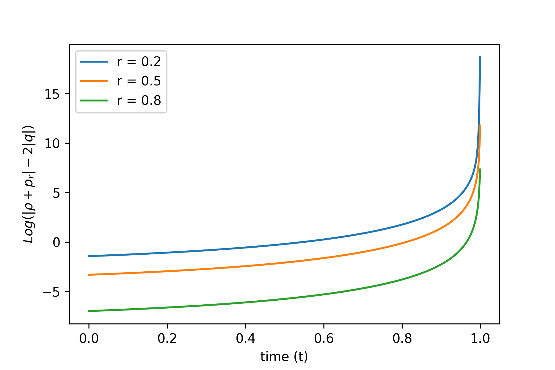
|ฯ+pr|โˆ’2โ€‹|q|โ‰ฅ0๐œŒsubscript๐‘๐‘Ÿ2๐‘ž0|\rho+p_{r}|-2|q|\geq 0 (39)
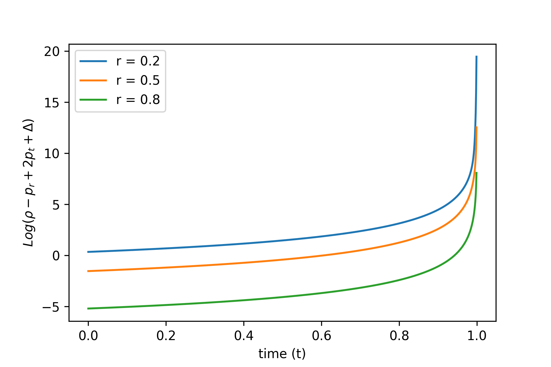
ฯโˆ’pr+2โ€‹pt+ฮ”โ‰ฅ0๐œŒsubscript๐‘๐‘Ÿ2subscript๐‘๐‘กฮ”0\rho-p_{r}+2p_{t}+\Delta\geq 0 (40)

where, ฮ”=(ฯ+pr)2โˆ’4โ€‹q2ฮ”superscript๐œŒsubscript๐‘๐‘Ÿ24superscript๐‘ž2\Delta=\sqrt{(\rho+p_{r})^{2}-4q^{2}}.

V.2 Weak energy condition

The weak energy condition must be obeyed for a physically acceptable model of gravitational collapse. The weak energy condition states that if ฮป0subscript๐œ†0\lambda_{0} signifies the eigenvalue corresponding to the time-like eigenvector, then โˆ’ฮป0โ‰ฅ0subscript๐œ†00-\lambda_{0}\geq 0 must be true. As a result, the shear-less fluidโ€™s weak energy condition becomes

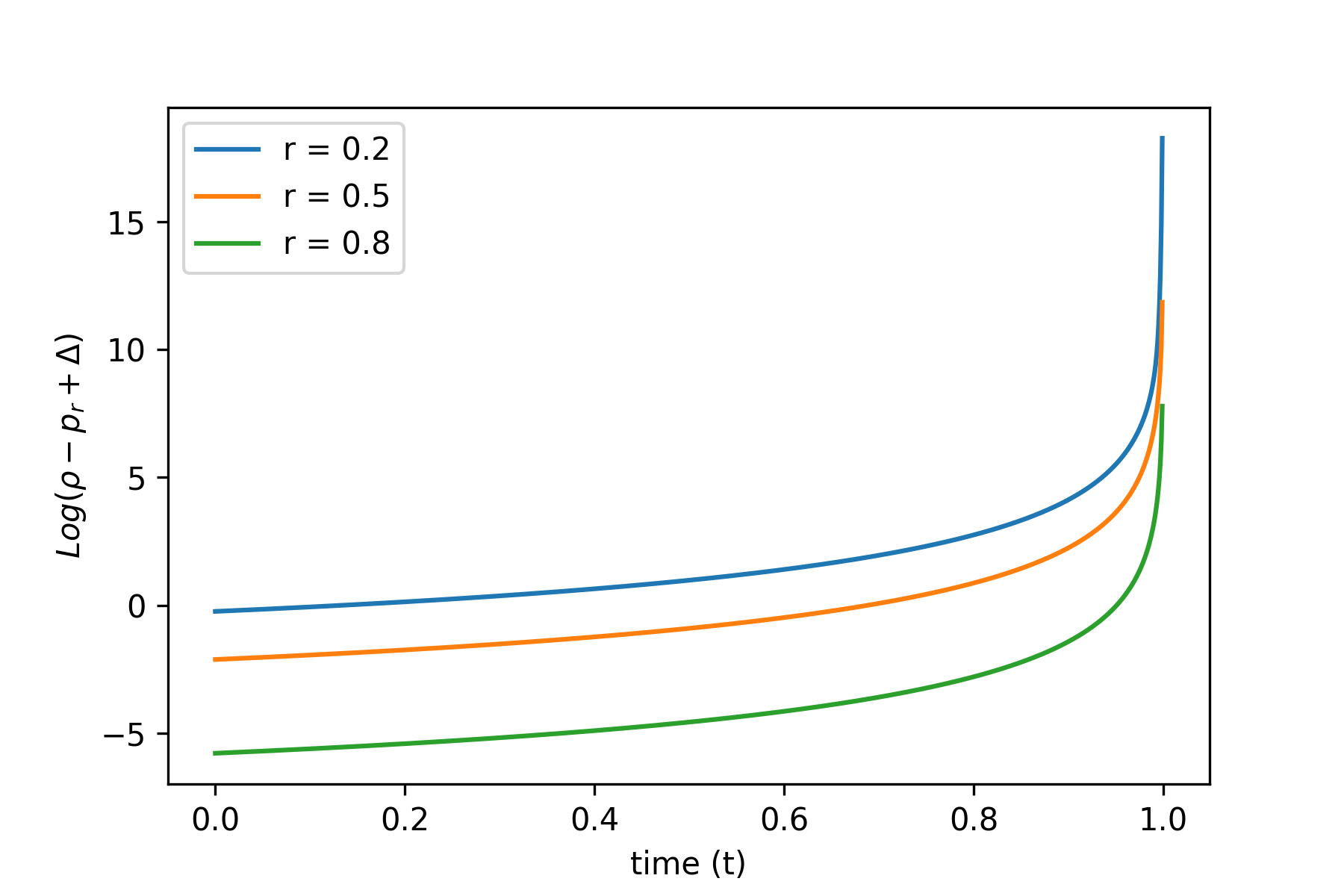
ฯโˆ’pr+ฮ”โ‰ฅ0๐œŒsubscript๐‘๐‘Ÿฮ”0\rho-p_{r}+\Delta\geq 0 (41)

V.3 Dominant energy conditions

Any physically acceptable model must also obey the dominant energy conditions. If ฮปisubscript๐œ†๐‘–\lambda_{i} signifies the eigenvalues corresponding to the space-like eigenvectors, then it must follow the condition given by ฮป0โ‰คฮปiโ‰คฮป0subscript๐œ†0subscript๐œ†๐‘–subscript๐œ†0\lambda_{0}\leq\lambda_{i}\leq\lambda_{0}. Thus, the dominant energy conditions for shear-less fluid can be written in terms of physical quantities of the star as follow

ฯโˆ’prโˆ’2โ€‹pt+ฮ”โ‰ฅ0๐œŒsubscript๐‘๐‘Ÿ2subscript๐‘๐‘กฮ”0\rho-p_{r}-2p_{t}+\Delta\geq 0 (42)
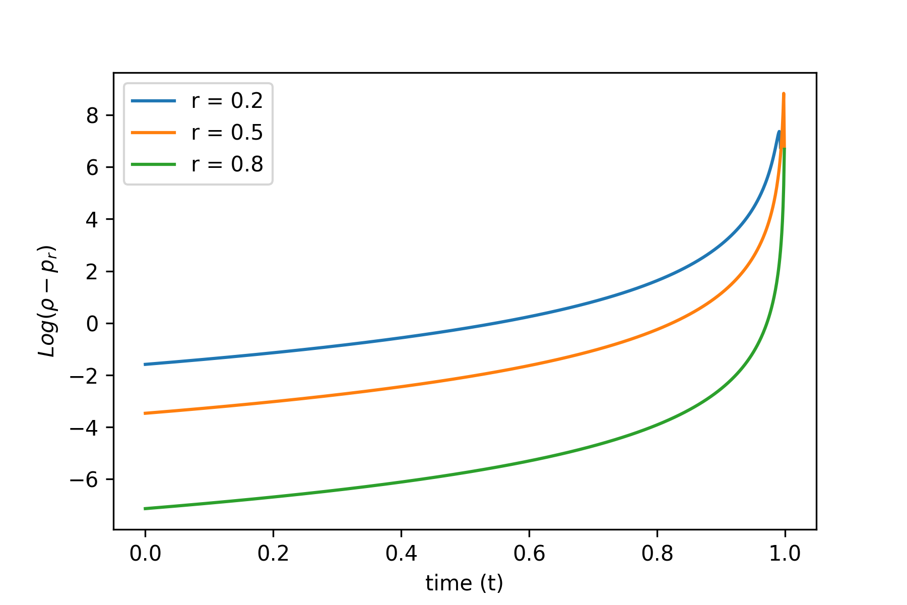
ฯโˆ’prโ‰ฅ0๐œŒsubscript๐‘๐‘Ÿ0\rho-p_{r}\geq 0 (43)

V.4 Strong energy condition

By imposing the last strong energy condition, a physically acceptable model can be found. The presence of a strong energy condition indicates that ฮป0+โˆ‘iฮปiโ‰ฅ0subscript๐œ†0subscript๐‘–subscript๐œ†๐‘–0\lambda_{0}+\sum_{i}\lambda_{i}\geq 0. Which implies that physical quantities of the star mast obey following condition

2โ€‹pt+ฮ”โ‰ฅ02subscript๐‘๐‘กฮ”02p_{t}+\Delta\geq 0 (44)

Thus, physically acceptable model of stars undergoing gravitational collapse can be found by imposing all energy conditions from (39) to (44).

VI Physical analysis of the model

In this section we present physical analysis for the different values of k๐‘˜k and m๐‘šm. Equations (35) to (38) represents analytical solutions for general case of R+fโ€‹(R)=R+kโ€‹Rm๐‘…๐‘“๐‘…๐‘…๐‘˜superscript๐‘…๐‘šR+f(R)=R+kR^{m}. Here we choose different values of k๐‘˜k and m๐‘šm and apply energy conditions for each case to generate physically acceptable models of gravitational collapse.

VI.1 Physical analysis with k=0๐‘˜0k=0

Firstly, we choose the value of k=0๐‘˜0k=0. So that the field equations becomes essentially of General Relativity. Thus, with k=0๐‘˜0k=0, equations (35) to (38) describes gravitational collapse in General Relativity. By putting k=0๐‘˜0k=0 in them we get the following analytical forms of physical quantities by choosing a=b=1๐‘Ž๐‘1a=b=1

ฯโ€‹(t,r)=(1โˆ’r)44โ€‹(1โˆ’t)2โ€‹(5โˆ’2โ€‹t)๐œŒ๐‘ก๐‘Ÿsuperscript1๐‘Ÿ44superscript1๐‘ก252๐‘ก\rho(t,r)=\frac{(1-r)^{4}}{4(1-t)^{2}}(5-2t) (45)
prโ€‹(t,r)=(1โˆ’r)44โ€‹(1โˆ’t)2โ€‹(3โˆ’2โ€‹t)subscript๐‘๐‘Ÿ๐‘ก๐‘Ÿsuperscript1๐‘Ÿ44superscript1๐‘ก232๐‘กp_{r}(t,r)=\frac{(1-r)^{4}}{4(1-t)^{2}}(3-2t) (46)
ptโ€‹(t,r)=(1โˆ’r)44โ€‹(1โˆ’t)2โ€‹(3โˆ’2โ€‹t)subscript๐‘๐‘ก๐‘ก๐‘Ÿsuperscript1๐‘Ÿ44superscript1๐‘ก232๐‘กp_{t}(t,r)=\frac{(1-r)^{4}}{4(1-t)^{2}}(3-2t) (47)
qโ€‹(t,r)=(1โˆ’r)42โ€‹(1โˆ’t)32๐‘ž๐‘ก๐‘Ÿsuperscript1๐‘Ÿ42superscript1๐‘ก32q(t,r)=\frac{(1-r)^{4}}{\sqrt{2}(1-t)^{\frac{3}{2}}} (48)

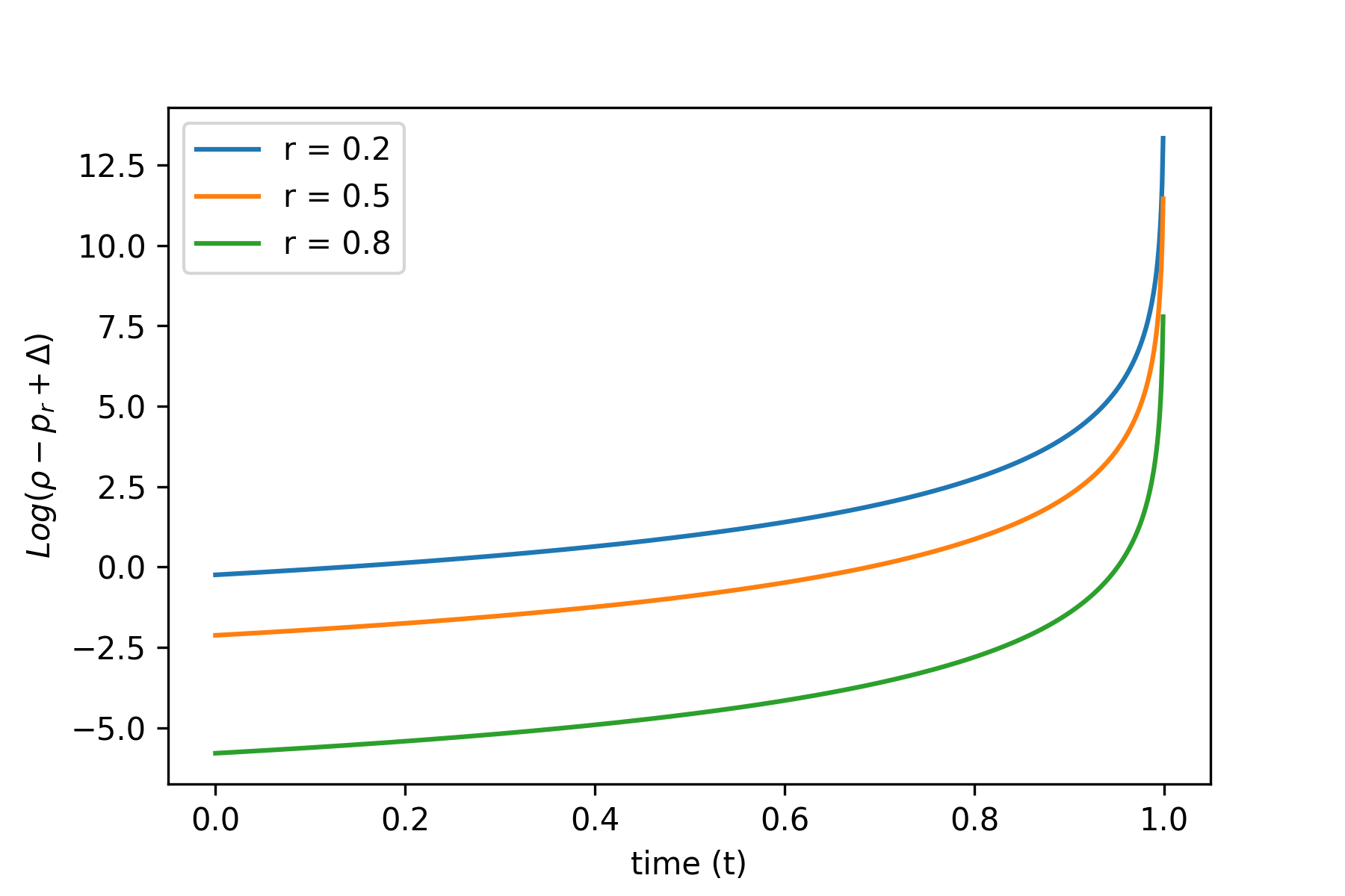
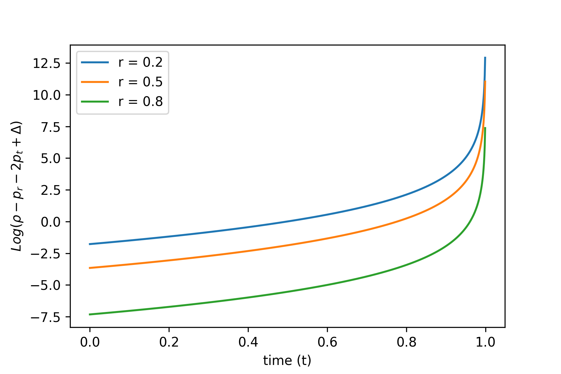
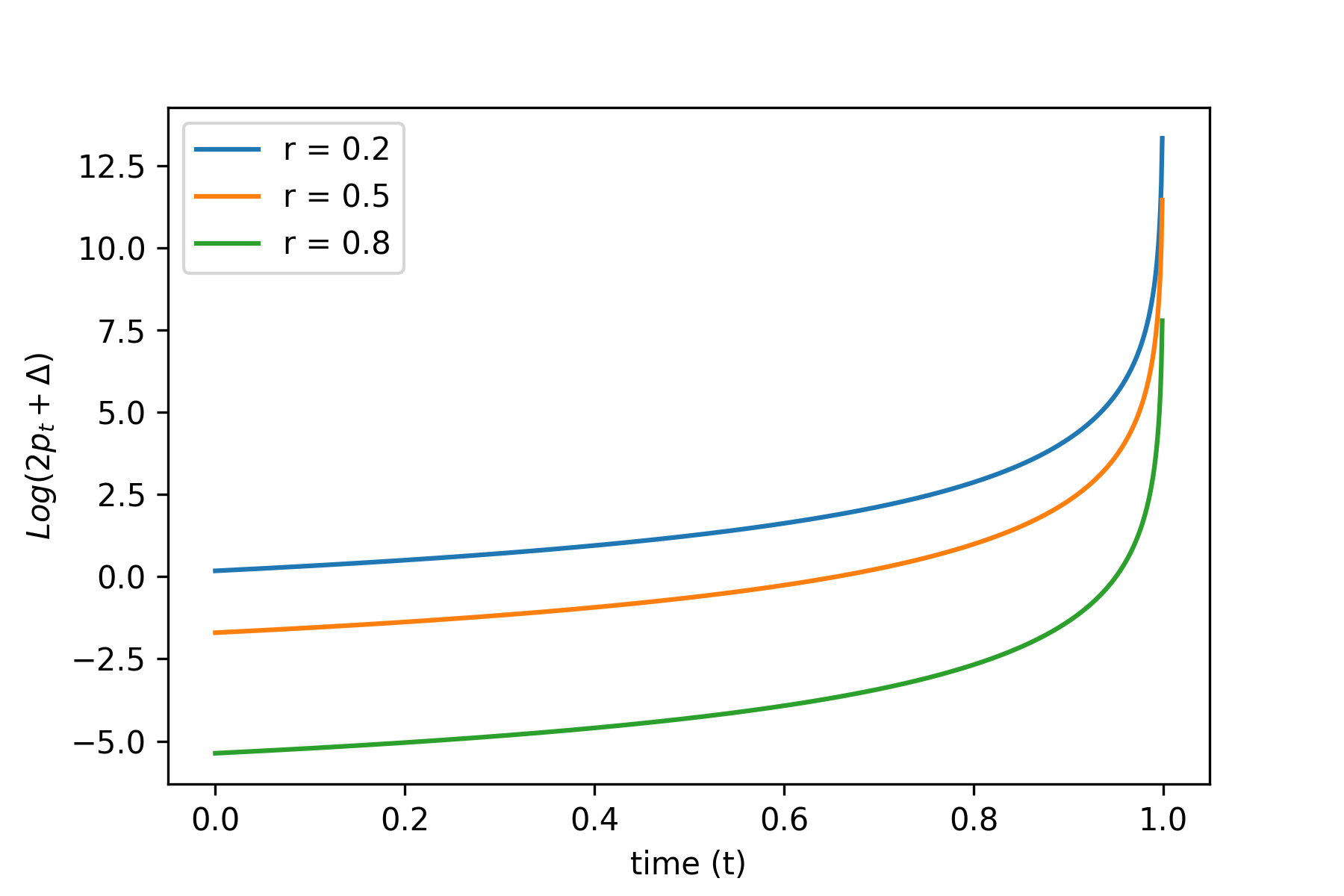
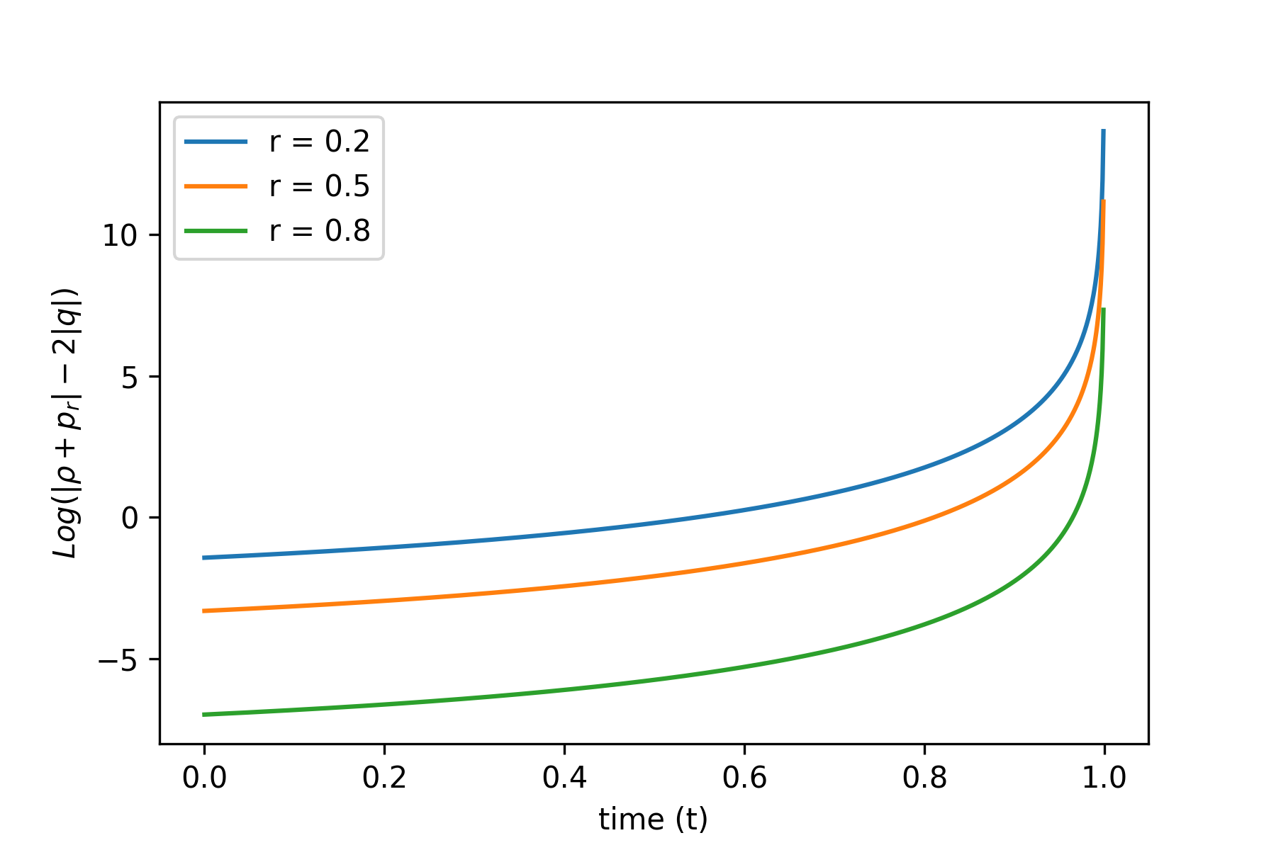
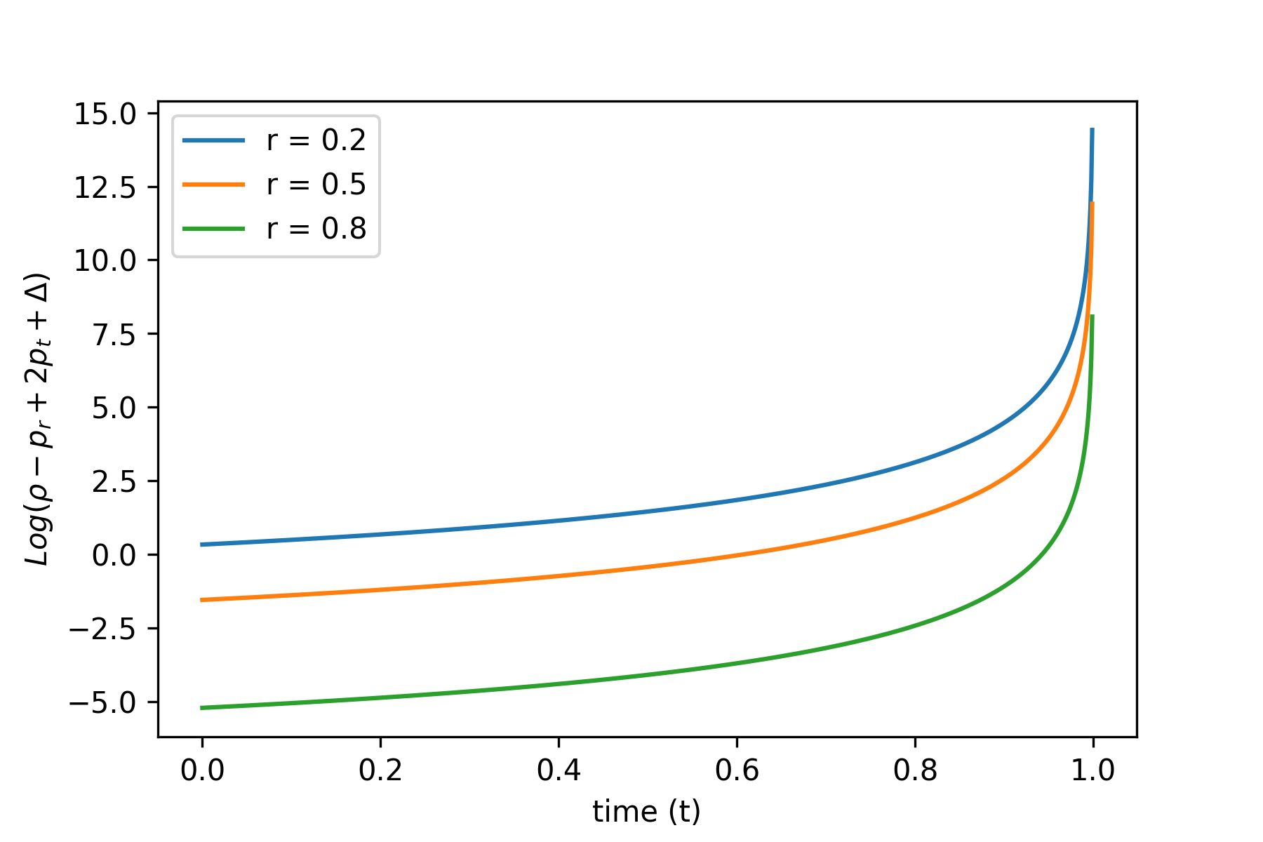
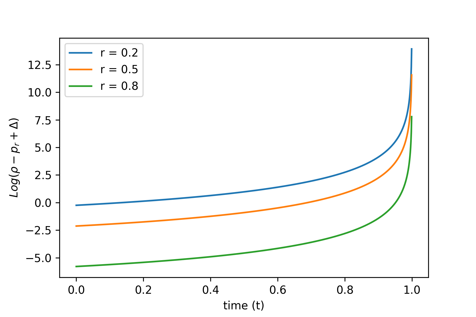
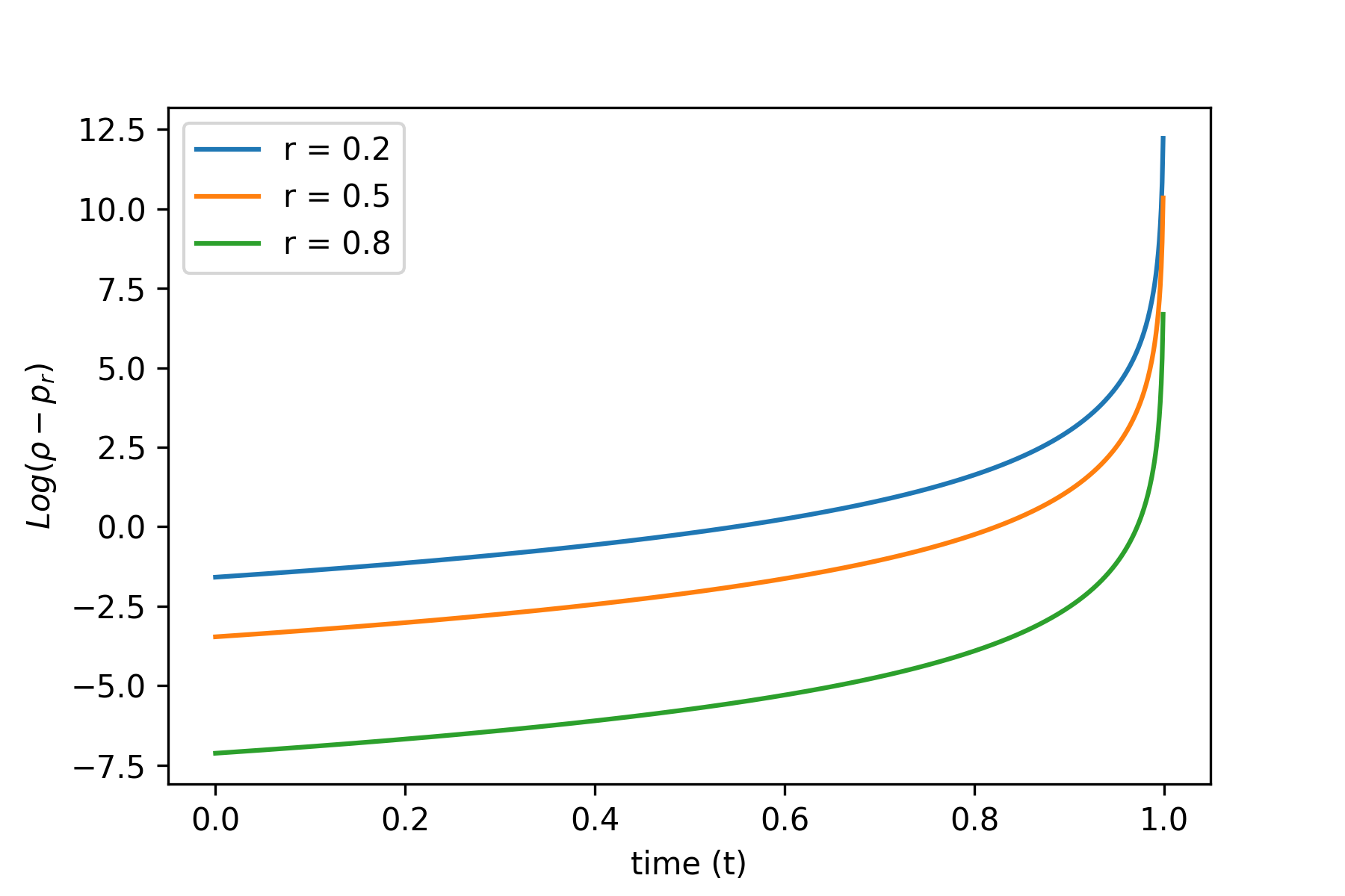
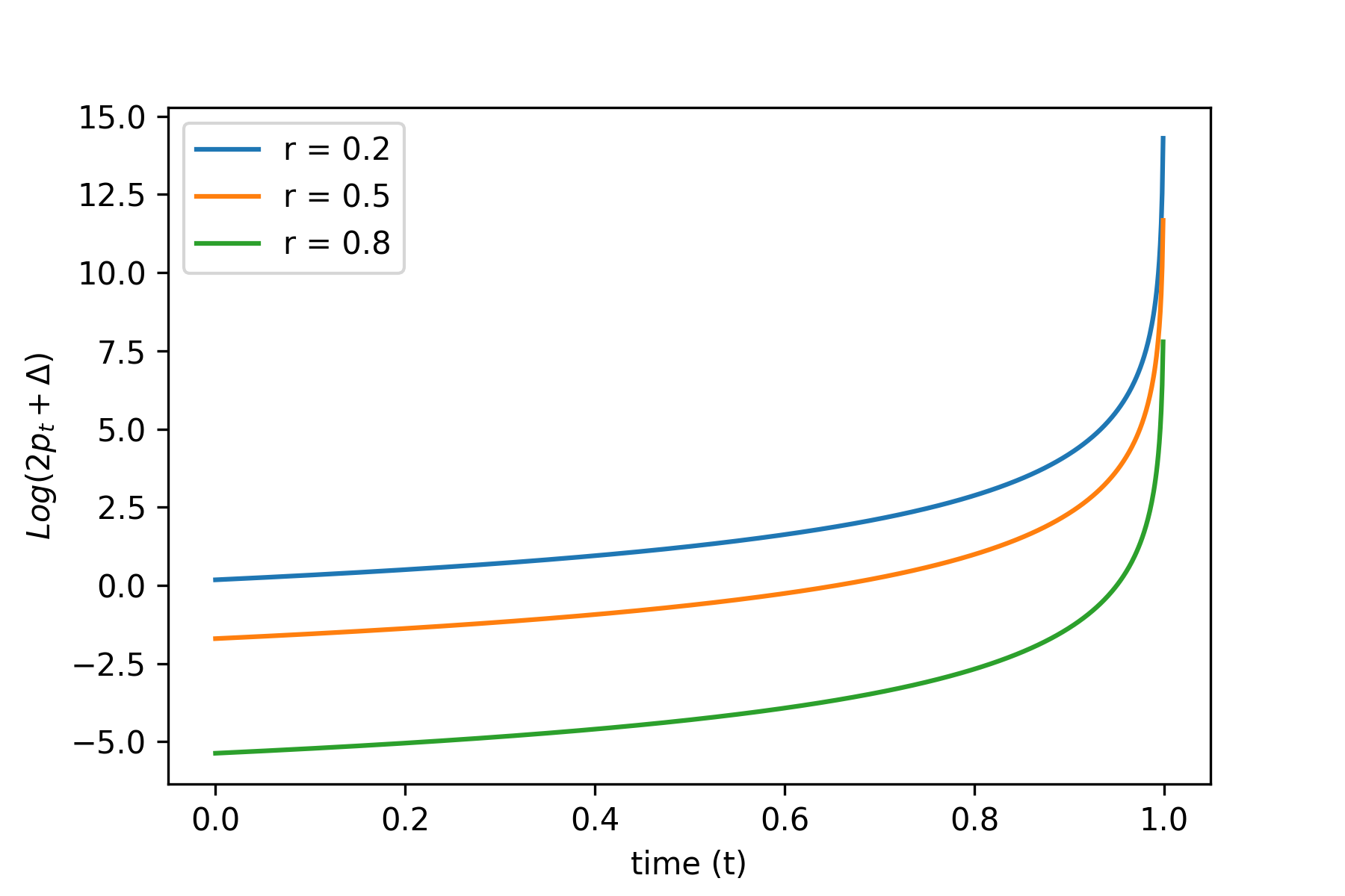
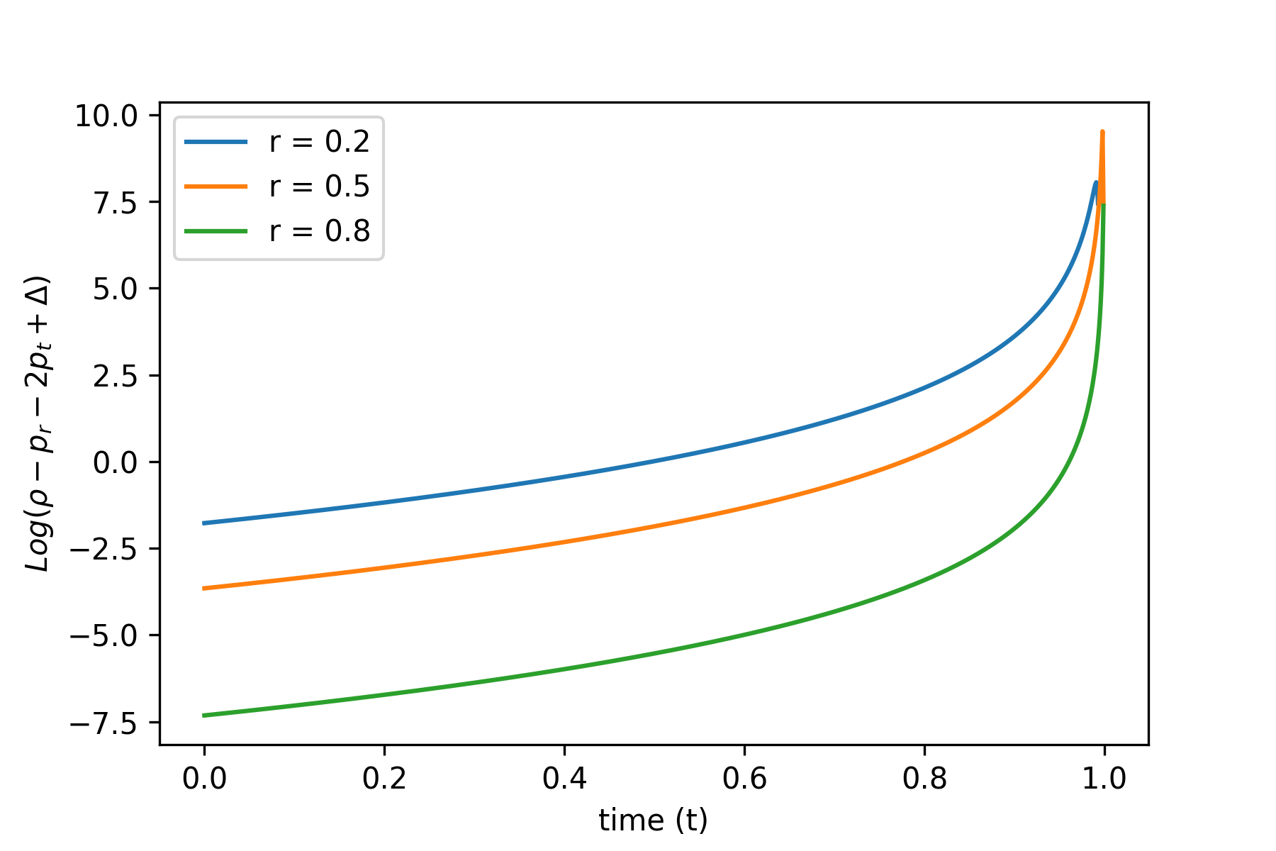
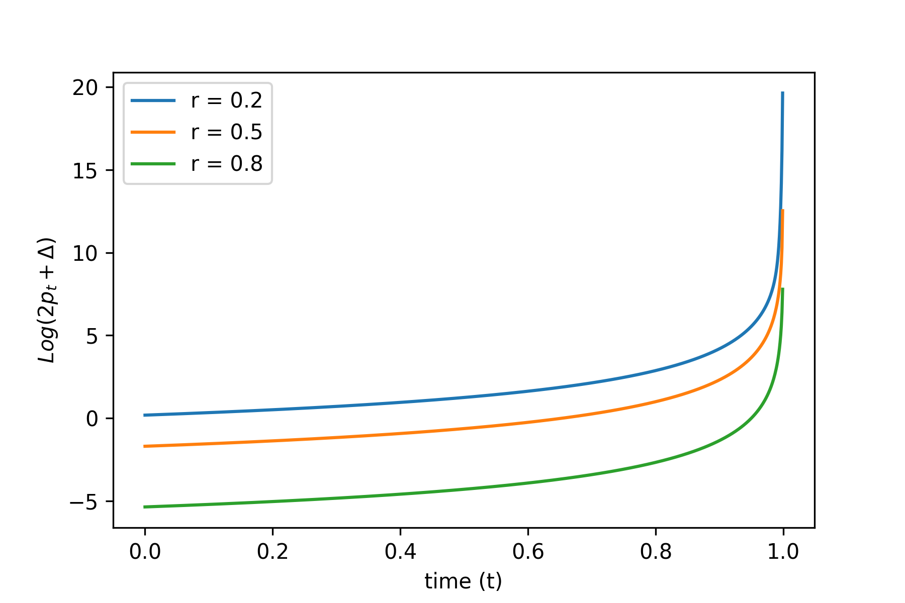
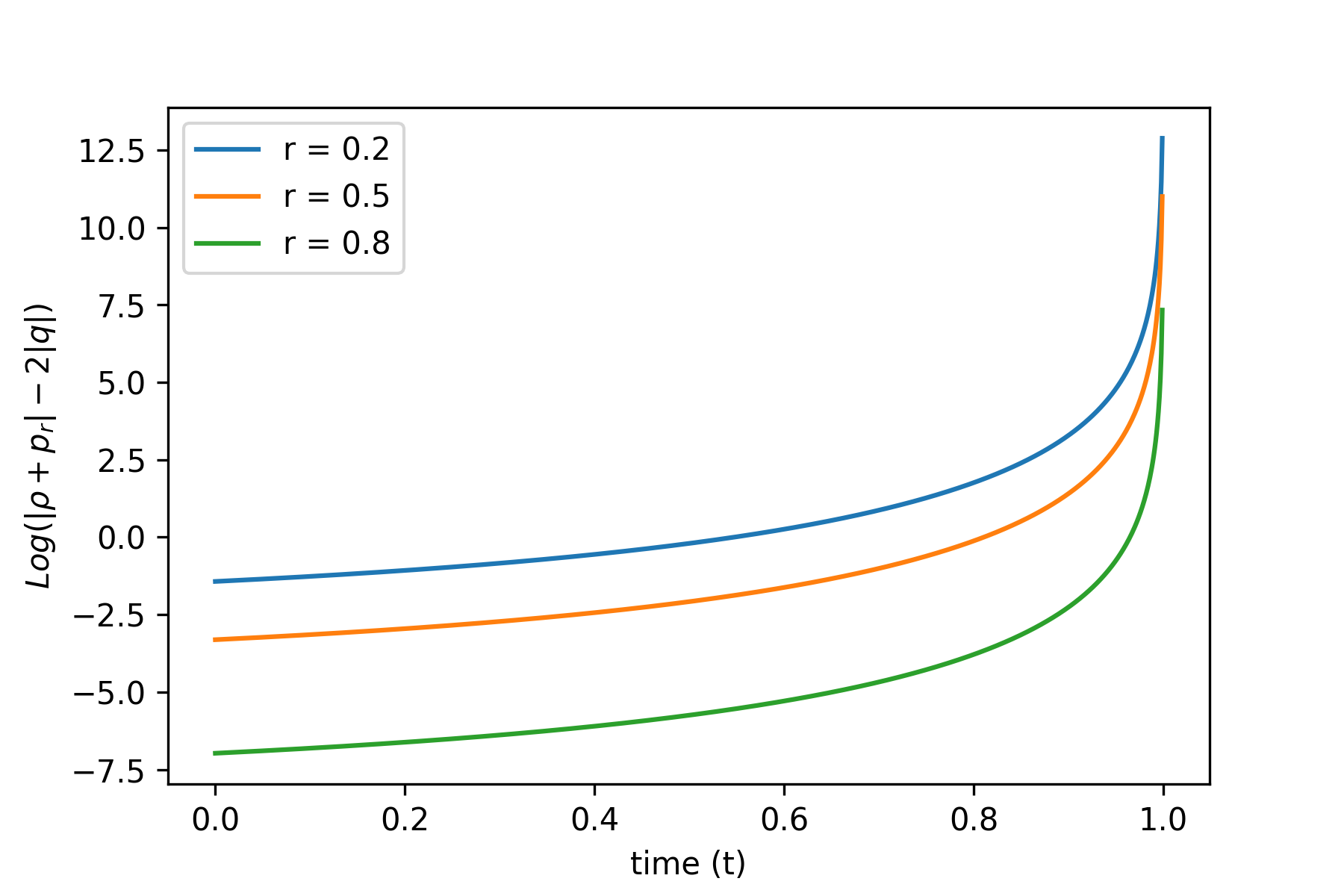
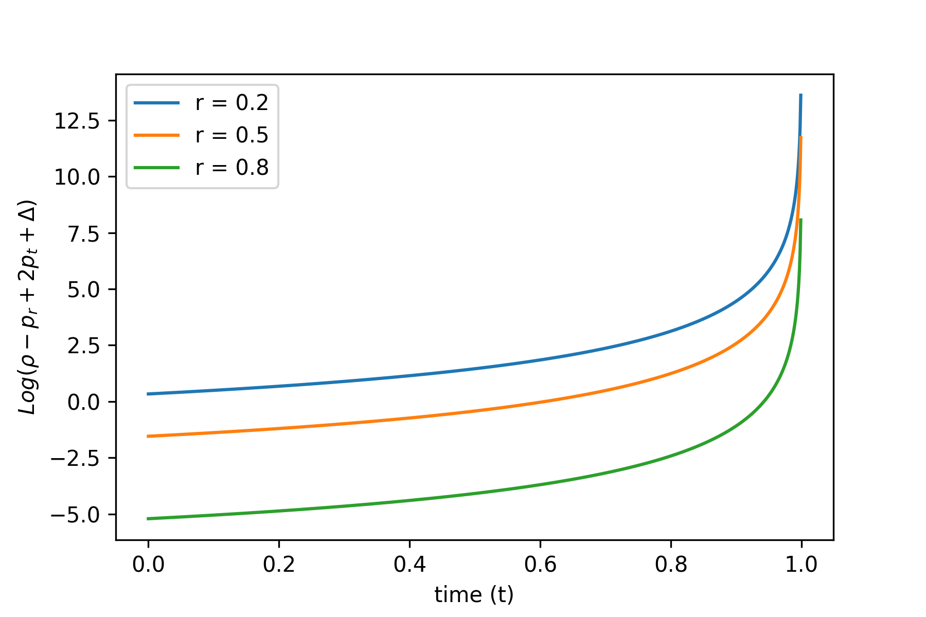
Equations (45) to (48) shows that gravitational collapse starts at t=0๐‘ก0t=0 and ends up in singularity t=1๐‘ก1t=1 with blowing up all physical quantities. It can be seen from the equations (46) and (47) that anisotropy of collapsing stars for k=0๐‘˜0k=0 identically vanishes for all time at all interior points of the star. However, it is not the case for the non-zero value of k๐‘˜k, providing the model in modified fโ€‹(R)๐‘“๐‘…f(R) gravity. Also, we plot all the energy conditions described in section V. All the graphs are presented in FIG 1 show that this model satisfies all the energy conditions, and thus it is physically acceptable.

Refer to caption
Refer to caption
Refer to caption
Refer to caption
Refer to caption
Refer to caption
Figure 1: Energy conditions for the model of gravitational collapse with k=0๐‘˜0k=0

VI.2 Physical analysis of the model fโ€‹(R)=kโ€‹R2๐‘“๐‘…๐‘˜superscript๐‘…2f(R)=kR^{2}

Now we choose the value of m=2๐‘š2m=2. Thus, the model becomes R+fโ€‹(R)=R+kโ€‹R2๐‘…๐‘“๐‘…๐‘…๐‘˜superscript๐‘…2R+f(R)=R+kR^{2}. We put the values of m=2๐‘š2m=2, k=10โˆ’3๐‘˜superscript103k=10^{-3}, and a=b=1๐‘Ž๐‘1a=b=1 in equations (35) to (38) and thus, the equations becomes

ฯโ€‹(t,r)=(1โˆ’r)44โ€‹(1โˆ’t)3โ€‹[(5โˆ’2โ€‹t)โ€‹(1โˆ’t)+kโ€‹(1โˆ’r)4โ€‹(8โˆ’2โ€‹t)]๐œŒ๐‘ก๐‘Ÿsuperscript1๐‘Ÿ44superscript1๐‘ก3delimited-[]52๐‘ก1๐‘ก๐‘˜superscript1๐‘Ÿ482๐‘ก\rho(t,r)=\frac{(1-r)^{4}}{4(1-t)^{3}}[(5-2t)(1-t)+k\left(1-r\right)^{4}(8-2t)] (49)
prโ€‹(t,r)=(1โˆ’r)44โ€‹(1โˆ’t)3โ€‹[(3โˆ’2โ€‹t)โ€‹(1โˆ’t)+kโ€‹(1โˆ’r)4โ€‹(28โˆ’22โ€‹t)]subscript๐‘๐‘Ÿ๐‘ก๐‘Ÿsuperscript1๐‘Ÿ44superscript1๐‘ก3delimited-[]32๐‘ก1๐‘ก๐‘˜superscript1๐‘Ÿ42822๐‘กp_{r}(t,r)=\frac{(1-r)^{4}}{4(1-t)^{3}}[(3-2t)(1-t)+k\left(1-r\right)^{4}(28-22t)] (50)
ptโ€‹(t,r)=(1โˆ’r)44โ€‹(1โˆ’t)3โ€‹[(3โˆ’2โ€‹t)โ€‹(1โˆ’t)โˆ’kโ€‹(1โˆ’r)4โ€‹(4โˆ’10โ€‹t)]subscript๐‘๐‘ก๐‘ก๐‘Ÿsuperscript1๐‘Ÿ44superscript1๐‘ก3delimited-[]32๐‘ก1๐‘ก๐‘˜superscript1๐‘Ÿ4410๐‘กp_{t}(t,r)=\frac{(1-r)^{4}}{4(1-t)^{3}}[(3-2t)(1-t)-k\left(1-r\right)^{4}(4-10t)] (51)
qโ€‹(t,r)=(1โˆ’r)42โ€‹(1โˆ’t)52โ€‹[1โˆ’t+6โ€‹kโ€‹(1โˆ’r)4]๐‘ž๐‘ก๐‘Ÿsuperscript1๐‘Ÿ42superscript1๐‘ก52delimited-[]1๐‘ก6๐‘˜superscript1๐‘Ÿ4q(t,r)=\frac{(1-r)^{4}}{\sqrt{2}(1-t)^{\frac{5}{2}}}[1-t+6k\left(1-r\right)^{4}] (52)

Equations (49) to (52) represents analytical solutions of gravitational collapse in R2superscript๐‘…2R^{2} corrected fโ€‹(R)๐‘“๐‘…f(R) gravity. Equations (49) to (52) shows that for this model also collapse starts at t=0๐‘ก0t=0 and it ends up in singularity at t=1๐‘ก1t=1, due to the choice of b=1๐‘1b=1. Equations (50) and (51) shows that anisotropy doesnโ€™t vanish at the interior of star, unlike vanishing anisotropy in case of collapse governed by general relativity. We plot all the energy conditions for this model in FIG 2. All the graphs presented in FIG 2. shows that this model satisfy all the energy conditions and thus it is physically acceptable.

Refer to caption
Refer to caption
Refer to caption
Refer to caption
Refer to caption
Refer to caption
Figure 2: Energy conditions for the model of gravitational collapse with fโ€‹(R)=kโ€‹R2๐‘“๐‘…๐‘˜superscript๐‘…2f(R)=kR^{2}

VI.3 Physical analysis of the model fโ€‹(R)=kโ€‹R4๐‘“๐‘…๐‘˜superscript๐‘…4f(R)=kR^{4}

Finally we choose R+fโ€‹(R)=R+kโ€‹R4๐‘…๐‘“๐‘…๐‘…๐‘˜superscript๐‘…4R+f(R)=R+kR^{4} model to describe gravitational collapse of compact stars. We put the values of m=4๐‘š4m=4, k=10โˆ’7๐‘˜superscript107k=10^{-7}, and a=b=1๐‘Ž๐‘1a=b=1 in equations (35) to (38) and thus, the equations becomes

ฯโ€‹(t,r)=(1โˆ’r)44โ€‹(1โˆ’t)5โ€‹[(5โˆ’2โ€‹t)โ€‹(1โˆ’t)3+kโ€‹(1โˆ’r)12โ€‹(286โˆ’226โ€‹t)]๐œŒ๐‘ก๐‘Ÿsuperscript1๐‘Ÿ44superscript1๐‘ก5delimited-[]52๐‘กsuperscript1๐‘ก3๐‘˜superscript1๐‘Ÿ12286226๐‘ก\rho(t,r)=\frac{(1-r)^{4}}{4(1-t)^{5}}[(5-2t)(1-t)^{3}+k\left(1-r\right)^{12}(286-226t)] (53)
prโ€‹(t,r)=(1โˆ’r)44โ€‹(1โˆ’t)5โ€‹[(3โˆ’2โ€‹t)โ€‹(1โˆ’t)3+kโ€‹(1โˆ’r)12โ€‹(282โˆ’142โ€‹t)]subscript๐‘๐‘Ÿ๐‘ก๐‘Ÿsuperscript1๐‘Ÿ44superscript1๐‘ก5delimited-[]32๐‘กsuperscript1๐‘ก3๐‘˜superscript1๐‘Ÿ12282142๐‘กp_{r}(t,r)=\frac{(1-r)^{4}}{4(1-t)^{5}}[(3-2t)(1-t)^{3}+k\left(1-r\right)^{12}(282-142t)] (54)
ptโ€‹(t,r)=(1โˆ’r)44โ€‹(1โˆ’t)5โ€‹[(3โˆ’2โ€‹t)โ€‹(1โˆ’t)3โˆ’kโ€‹(1โˆ’r)12โ€‹(102โˆ’242โ€‹t)]subscript๐‘๐‘ก๐‘ก๐‘Ÿsuperscript1๐‘Ÿ44superscript1๐‘ก5delimited-[]32๐‘กsuperscript1๐‘ก3๐‘˜superscript1๐‘Ÿ12102242๐‘กp_{t}(t,r)=\frac{(1-r)^{4}}{4(1-t)^{5}}[(3-2t)(1-t)^{3}-k\left(1-r\right)^{12}(102-242t)] (55)
qโ€‹(t,r)=(1โˆ’r)42โ€‹(1โˆ’t)92โ€‹[(1โˆ’t)3+92โ€‹kโ€‹(1โˆ’r)12]๐‘ž๐‘ก๐‘Ÿsuperscript1๐‘Ÿ42superscript1๐‘ก92delimited-[]superscript1๐‘ก392๐‘˜superscript1๐‘Ÿ12q(t,r)=\frac{(1-r)^{4}}{\sqrt{2}(1-t)^{\frac{9}{2}}}[(1-t)^{3}+92k\left(1-r\right)^{12}] (56)

Equations (53) to (56) represents analytical solutions of gravitational collapse in R4superscript๐‘…4R^{4} corrected fโ€‹(R)๐‘“๐‘…f(R) gravity. The gravitational collapse starts at t=0๐‘ก0t=0 and due to choice of b=1๐‘1b=1, this model also governs the end of collapse in singularity at t=1๐‘ก1t=1. However, due to higher-order correction in the gravitational model, the stronger gravitational pull crunches matter with more power. This can be seen by comparing scales of physical quantities in R2superscript๐‘…2R^{2} corrected and R4superscript๐‘…4R^{4} corrected gravity. Equations (54) and (55) show that anisotropy does not vanish for this case also, as was the case for R2superscript๐‘…2R^{2} corrected gravity. In the following section, we show that anisotropy has to be taken into account for describing the gravitational collapse of stars in the general fโ€‹(R)๐‘“๐‘…f(R) gravity model. We also plot all the energy conditions for this model in FIG 3. The graphs show that this model satisfies all the energy conditions, and thus it is physically acceptable.

Refer to caption
Refer to caption
Refer to caption
Refer to caption
Refer to caption
Refer to caption
Figure 3: Energy conditions for the model of gravitational collapse with fโ€‹(R)=kโ€‹R4๐‘“๐‘…๐‘˜superscript๐‘…4f(R)=kR^{4}

VII Physical properties of gravitationally collapsing stars

In section IV, we have computed the energy density, pressures, and heat flux density of gravitationally collapsing stars. The gravitational collapse in fโ€‹(R)๐‘“๐‘…f(R) gravity also exhibits other useful properties, which are useful to study the inherent nature of such gravitationally collapsing compact stars. Thus, we will study the other useful properties of gravitationally collapsing stars such as shear and anisotropic behavior of matter undergoing gravitational collapse and formation of the apparent horizon by calculating various quantities like 4-velocity, 4-acceleration and expansion parameter of matter, the projection tensor, and shearing tensor. The 4-velocity and the radial vector used in (3) for the space-time metric (5) and having functions yโ€‹(r)๐‘ฆ๐‘Ÿy(r) and cโ€‹(t)๐‘๐‘กc(t) given by (33) are given by

uฮฑ=((1โˆ’ra)2,0,0,0)andvฮฑ=(0,aโ€‹(1โˆ’ra)32โ€‹2โ€‹1โˆ’bโ€‹t,0,0)formulae-sequencesuperscript๐‘ข๐›ผsuperscript1๐‘Ÿ๐‘Ž2000andsuperscript๐‘ฃ๐›ผ0๐‘Žsuperscript1๐‘Ÿ๐‘Ž3221๐‘๐‘ก00u^{\alpha}=\left(\left(1-\frac{r}{a}\right)^{2},0,0,0\right)\quad\mathrm{and}\quad v^{\alpha}=\left(0,\frac{a\left(1-\frac{r}{a}\right)^{3}}{2\sqrt{2}\sqrt{1-bt}},0,0\right) (57)

The 4-acceleration of the fluid can be computed from the following equation

aฮฑ=uฮฒโ€‹(โˆ‡ฮฒuฮฑ)superscript๐‘Ž๐›ผsuperscript๐‘ข๐›ฝsubscriptโˆ‡๐›ฝsuperscript๐‘ข๐›ผa^{\alpha}=u^{\beta}(\nabla_{\beta}u^{\alpha}) (58)

which has the following non-zero radial component

a1=aโ€‹(1โˆ’ra)54โ€‹(1โˆ’bโ€‹t)superscript๐‘Ž1๐‘Žsuperscript1๐‘Ÿ๐‘Ž541๐‘๐‘กa^{1}=\frac{a\left(1-\frac{r}{a}\right)^{5}}{4(1-bt)} (59)

Now we computes the expansion parameter as follow

ฮ˜=โˆ‡ฮฑuฮฑ=โˆ’3โ€‹bโ€‹(1โˆ’ra)22โ€‹(1โˆ’bโ€‹t)ฮ˜subscriptโˆ‡๐›ผsuperscript๐‘ข๐›ผ3๐‘superscript1๐‘Ÿ๐‘Ž221๐‘๐‘ก\Theta=\nabla_{\alpha}u^{\alpha}=-\frac{3b\left(1-\frac{r}{a}\right)^{2}}{2(1-bt)} (60)

The shear tensor can be computed from the following identity

ฯƒฮฑโ€‹ฮฒ=u(ฮฑ;ฮฒ)+a(ฮฑโ€‹uฮฒ)โˆ’13โ€‹ฮ˜โ€‹(gฮฑโ€‹ฮฒ+uฮฑโ€‹uฮฒ)\sigma_{\alpha\beta}=u_{(\alpha;\beta)}+a_{(\alpha}u_{\beta)}-\frac{1}{3}\Theta(g_{\alpha\beta}+u_{\alpha}u_{\beta}) (61)

where hฮฑโ€‹ฮฒ=gฮฑโ€‹ฮฒ+uฮฑโ€‹uฮฒsubscriptโ„Ž๐›ผ๐›ฝsubscript๐‘”๐›ผ๐›ฝsubscript๐‘ข๐›ผsubscript๐‘ข๐›ฝh_{\alpha\beta}=g_{\alpha\beta}+u_{\alpha}u_{\beta} is known as projection tensor. From equation (61), we compute the components of shearing tensor as follow

ฯƒ00=โˆ’bโ€‹(1โˆ’ra)22โ€‹(1โˆ’bโ€‹t)โ€‹(โˆ’1(1โˆ’ra)4+1(1โˆ’ra)4)=0subscript๐œŽ00๐‘superscript1๐‘Ÿ๐‘Ž221๐‘๐‘ก1superscript1๐‘Ÿ๐‘Ž41superscript1๐‘Ÿ๐‘Ž40\sigma_{00}=\frac{-b\left(1-\frac{r}{a}\right)^{2}}{2(1-bt)}\left(-\frac{1}{\left(1-\frac{r}{a}\right)^{4}}+\frac{1}{\left(1-\frac{r}{a}\right)^{4}}\right)=0 (62)
ฯƒ01=ฯƒ10=1aโ€‹(1โˆ’ra)3โˆ’1aโ€‹(1โˆ’ra)3=0subscript๐œŽ01subscript๐œŽ101๐‘Žsuperscript1๐‘Ÿ๐‘Ž31๐‘Žsuperscript1๐‘Ÿ๐‘Ž30\sigma_{01}=\sigma_{10}=\frac{1}{a\left(1-\frac{r}{a}\right)^{3}}-\frac{1}{a\left(1-\frac{r}{a}\right)^{3}}=0 (63)
ฯƒ11=2โ€‹(โˆ’b2)โ€‹(4a2)(1โˆ’ra)4โˆ’(1โˆ’ra)2โ€‹(โˆ’b2)(1โˆ’bโ€‹t)โ€‹(2โ€‹(1โˆ’bโ€‹t)โ€‹4a2(1โˆ’ra)6)=0subscript๐œŽ112๐‘24superscript๐‘Ž2superscript1๐‘Ÿ๐‘Ž4superscript1๐‘Ÿ๐‘Ž2๐‘21๐‘๐‘ก21๐‘๐‘ก4superscript๐‘Ž2superscript1๐‘Ÿ๐‘Ž60\sigma_{11}=\frac{2(-\frac{b}{2})(\frac{4}{a^{2}})}{\left(1-\frac{r}{a}\right)^{4}}-\frac{\left(1-\frac{r}{a}\right)^{2}(-\frac{b}{2})}{(1-bt)}\left(\frac{2(1-bt)\frac{4}{a^{2}}}{\left(1-\frac{r}{a}\right)^{6}}\right)=0 (64)
ฯƒ22=(โˆ’b2)(1โˆ’ra)2โˆ’(โˆ’b2)โ€‹(1โˆ’ra)21โˆ’bโ€‹tโ€‹(1โˆ’bโ€‹t(1โˆ’ra)4)=0subscript๐œŽ22๐‘2superscript1๐‘Ÿ๐‘Ž2๐‘2superscript1๐‘Ÿ๐‘Ž21๐‘๐‘ก1๐‘๐‘กsuperscript1๐‘Ÿ๐‘Ž40\sigma_{22}=\frac{(-\frac{b}{2})}{\left(1-\frac{r}{a}\right)^{2}}-\frac{(-\frac{b}{2})\left(1-\frac{r}{a}\right)^{2}}{1-bt}\left(\frac{1-bt}{\left(1-\frac{r}{a}\right)^{4}}\right)=0 (65)
ฯƒ33=(โˆ’b2)(1โˆ’ra)2โ€‹sโ€‹iโ€‹n2โ€‹ฮธโˆ’(โˆ’b2)โ€‹(1โˆ’ra)21โˆ’bโ€‹tโ€‹(1โˆ’bโ€‹t(1โˆ’ra)4)โ€‹sโ€‹iโ€‹n2โ€‹ฮธ=0subscript๐œŽ33๐‘2superscript1๐‘Ÿ๐‘Ž2๐‘ ๐‘–superscript๐‘›2๐œƒ๐‘2superscript1๐‘Ÿ๐‘Ž21๐‘๐‘ก1๐‘๐‘กsuperscript1๐‘Ÿ๐‘Ž4๐‘ ๐‘–superscript๐‘›2๐œƒ0\sigma_{33}=\frac{(-\frac{b}{2})}{\left(1-\frac{r}{a}\right)^{2}}sin^{2}\theta-\frac{(-\frac{b}{2})\left(1-\frac{r}{a}\right)^{2}}{1-bt}\left(\frac{1-bt}{\left(1-\frac{r}{a}\right)^{4}}\right)sin^{2}\theta=0 (66)

Other components of the shearing tensor (61) also vanish due to the vanishing of individual parts. Thus, all components including (62) to (66) vanishes. Thus, the prior assumption of vanishing shear components holds for the study. It is important to note that the vanishing shear is only possible if gravitationally collapsing stars are being studied in the separable form of the interior space-time metric. The gravitational collapse of compact stars described by the non-separable form of interior metric involves the shear, and thus it has a non-zero shearing tensor. The detailed study of the gravitational collapse in the non-separable form of interior metric considering shear and its evolution is given in the reference 2008GReGr..40.2149P .

Now, we compute the anisotropy (S)๐‘†(S) of the stars undergoing the gravitational collapse described by the modified R+fโ€‹(R)=R+kโ€‹Rm๐‘…๐‘“๐‘…๐‘…๐‘˜superscript๐‘…๐‘šR+f(R)=R+kR^{m} gravity model under consideration. From equation (7) and (8) we have the following identity,

S=prโˆ’pt=fRโ€ฒโ€‹(yโ€ฒโฃ2+yโ€‹yโ€ฒโ€ฒ)2โ€‹yโ€‹yโ€ฒโฃ3โ€‹c2โˆ’fRโ€ฒโ€ฒ2โ€‹c2โ€‹yโ€ฒโฃ2๐‘†subscript๐‘๐‘Ÿsubscript๐‘๐‘กsuperscriptsubscript๐‘“๐‘…โ€ฒsuperscript๐‘ฆโ€ฒ2๐‘ฆsuperscript๐‘ฆโ€ฒโ€ฒ2๐‘ฆsuperscript๐‘ฆโ€ฒ3superscript๐‘2superscriptsubscript๐‘“๐‘…โ€ฒโ€ฒ2superscript๐‘2superscript๐‘ฆโ€ฒ2S=p_{r}-p_{t}=\frac{f_{R}^{\prime}(y^{\prime 2}+yy^{\prime\prime})}{2yy^{\prime 3}c^{2}}-\frac{f_{R}^{\prime\prime}}{2c^{2}y^{\prime 2}} (67)

For the model fโ€‹(R)=kโ€‹Rm๐‘“๐‘…๐‘˜superscript๐‘…๐‘šf(R)=kR^{m}, the values of fRโ€ฒsuperscriptsubscript๐‘“๐‘…โ€ฒf_{R}^{\prime} and fRโ€ฒโ€ฒsuperscriptsubscript๐‘“๐‘…โ€ฒโ€ฒf_{R}^{\prime\prime} is given by

fRโ€ฒ=โˆ’kโ€‹(2โ€‹m)โ€‹(mโˆ’1)โ€‹Rmโˆ’1โ€‹yโ€ฒysuperscriptsubscript๐‘“๐‘…โ€ฒ๐‘˜2๐‘š๐‘š1superscript๐‘…๐‘š1superscript๐‘ฆโ€ฒ๐‘ฆf_{R}^{\prime}=-k(2m)(m-1)R^{m-1}\frac{y^{\prime}}{y} (68)
fRโ€ฒโ€ฒ=kโ€‹Rmโˆ’1โ€‹[2โ€‹mโ€‹(mโˆ’1)โ€‹(2โ€‹mโˆ’1)โ€‹yโ€ฒโฃ2y2โˆ’2โ€‹mโ€‹(mโˆ’1)โ€‹yโ€ฒโ€ฒy]superscriptsubscript๐‘“๐‘…โ€ฒโ€ฒ๐‘˜superscript๐‘…๐‘š1delimited-[]2๐‘š๐‘š12๐‘š1superscript๐‘ฆโ€ฒ2superscript๐‘ฆ22๐‘š๐‘š1superscript๐‘ฆโ€ฒโ€ฒ๐‘ฆf_{R}^{\prime\prime}=kR^{m-1}\left[2m(m-1)(2m-1)\frac{y^{\prime 2}}{y^{2}}-2m(m-1)\frac{y^{\prime\prime}}{y}\right] (69)

Using equations (68) and (69) in equation (67), we compute the anisotropy as follow

S=prโˆ’pt=kโ€‹(2โ€‹m2)โ€‹(mโˆ’1)โ€‹Rm๐‘†subscript๐‘๐‘Ÿsubscript๐‘๐‘ก๐‘˜2superscript๐‘š2๐‘š1superscript๐‘…๐‘šS=p_{r}-p_{t}=k(2m^{2})(m-1)R^{m} (70)

The anisotropy S๐‘†S can be written in terms of space-time coordinate by utilizing equation (34) in (70) as follow

S=prโˆ’pt=kโ€‹(โˆ’1)mโ€‹(2โ€‹m2)โ€‹(mโˆ’1)โ€‹(1โˆ’ra)4โ€‹m(1โˆ’bโ€‹t)m๐‘†subscript๐‘๐‘Ÿsubscript๐‘๐‘ก๐‘˜superscript1๐‘š2superscript๐‘š2๐‘š1superscript1๐‘Ÿ๐‘Ž4๐‘šsuperscript1๐‘๐‘ก๐‘šS=p_{r}-p_{t}=k(-1)^{m}(2m^{2})(m-1)\frac{\left(1-\frac{r}{a}\right)^{4}m}{(1-bt)^{m}} (71)

Equation (70) shows that the anisotropy can vanish for k=0๐‘˜0k=0 only, in which case the solutions will reduce to GR. This fact can also be observed by equations (45) to (48). Thus, for the case of modified fโ€‹(R)๐‘“๐‘…f(R) gravity, we have to consider the anisotropic behavior of gravitationally collapsing stars described by the interior metric (5). Equation (71) shows that anisotropy does not vanish at the center of the gravitationally collapsing star, instead of vanishing central anisotropy for the stable, compact stars. Thus, it shows that extra curvature source (4) in fโ€‹(R)๐‘“๐‘…f(R) gravity forces the matter distribution to be anisotropic in nature for gravitationally collapsing stars described by the interior space-time (5).

Now we investigate the formation of the apparent horizon and singularity formation for gravitational collapse of compact stars with the model of fโ€‹(R)๐‘“๐‘…f(R) gravity under consideration. From equations (33) and (34), it can be seen that the gravitational collapse ends in singularity at t=1b๐‘ก1๐‘t=\frac{1}{b} when cโ€‹(t)=0๐‘๐‘ก0c(t)=0 and Ricci scalar diverges at all co-moving radii. Now the question is that whether the singularity is naked or the horizon is formed before the observers can see the formation of a singularity. In the second case, there will be a black hole when the horizon is formed while gravitational collapse continues to the formation of a singularity. Whether the singularity will be naked or not can be investigated by solving the equation of formation of an apparent horizon as follow

gฮฑโ€‹ฮฒโ€‹โˆ‚ฮฑ(cโ€‹(t)2โ€‹yโ€‹(r)2)โ€‹โˆ‚ฮฒ(cโ€‹(t)2โ€‹yโ€‹(r)2)=0superscript๐‘”๐›ผ๐›ฝsubscript๐›ผ๐‘superscript๐‘ก2๐‘ฆsuperscript๐‘Ÿ2subscript๐›ฝ๐‘superscript๐‘ก2๐‘ฆsuperscript๐‘Ÿ20g^{\alpha\beta}\partial_{\alpha}(c(t)^{2}y(r)^{2})\partial_{\beta}(c(t)^{2}y(r)^{2})=0 (72)

We use the general forms of yโ€‹(r)๐‘ฆ๐‘Ÿy(r) and cโ€‹(t)๐‘๐‘กc(t) as obtained in equation (33) and solve equation (72) as follow

th=4โˆ’2โ€‹b24โ€‹bsubscript๐‘กโ„Ž42superscript๐‘24๐‘t_{h}=\frac{4-2b^{2}}{4b} (73)

Where thsubscript๐‘กโ„Žt_{h} is the time at which horizon is formed. For b=1๐‘1b=1, the time when horizon is formed is th=12subscript๐‘กโ„Ž12t_{h}=\frac{1}{2}. Thus, for the particular solution (33) of interior space-time metric describing gravitational collapse with b=1๐‘1b=1, the horizon is formed at t=12๐‘ก12t=\frac{1}{2}. The particular solution with b=1๐‘1b=1 is of interest because it describes completely physical collapse satisfying all energy conditions as well as investigated in section 6 for gravitational collapse model Gโ€‹R๐บ๐‘…GR, R+kโ€‹R2๐‘…๐‘˜superscript๐‘…2R+kR^{2} and R+kโ€‹R4๐‘…๐‘˜superscript๐‘…4R+kR^{4} gravity. In that case, all observers will see the formation of the horizon before the singularity forms, and thus singularity will be hidden behind the horizon. Thus, observers for those particular cases of gravitational collapse will see that gravitational collapse is started at t=0๐‘ก0t=0 and horizon is formed at t=12๐‘ก12t=\frac{1}{2}, before the formation of singularity at t=1๐‘ก1t=1. However, it should be noted that it is not the only possible physically acceptable solution. We have chosen this class of solutions with b=1๐‘1b=1. However, for different classes of solutions satisfying all energy conditions with different values of b๐‘b is maybe possible. For different solutions, the horizon and singularity will be formed at different times or gravitational collapse may also end in naked singularity as can be investigated from equation (73).

VIII Discussion

In this paper, we obtained exact solutions describing gravitational collapse of compact stars in R+fโ€‹(R)=R+kโ€‹Rm๐‘…๐‘“๐‘…๐‘…๐‘˜superscript๐‘…๐‘šR+f(R)=R+kR^{m} gravity. We solved field equations of gravitational collapse in fโ€‹(R)๐‘“๐‘…f(R) gravity by considering junction conditions and implementing the method of R๐‘…R matching to ensure the continuity of the Ricci scalar and its derivatives across the matching hypersurface. These extra junction conditions restrict the physically possible solutions greatly, and thus, there are not many exact solutions are available for the problem in the literature. Recently some exact solutions have been developed by some authors, but the problem is considered only for the restricted class of fโ€‹(R)๐‘“๐‘…f(R) model.

Thus, in this paper, we formulated the exact solutions describing the gravitational collapse of compact stars in general and physically important model of fโ€‹(R)๐‘“๐‘…f(R) gravity. We then investigated the values of model parameters such that they satisfy all necessary energy conditions. We have demonstrated the modelโ€™s validity for Gโ€‹R๐บ๐‘…GR, R+kโ€‹R2๐‘…๐‘˜superscript๐‘…2R+kR^{2} and R+kโ€‹R4๐‘…๐‘˜superscript๐‘…4R+kR^{4} gravity. However, the model is utterly physical for any order of corrections in fโ€‹(R)=kโ€‹Rm๐‘“๐‘…๐‘˜superscript๐‘…๐‘šf(R)=kR^{m} gravity. We have presented a comprehensive graphical analysis of energy conditions for each case and explained all case and their consequences. We also explained how the gravitational collapse scenario is different for Gโ€‹R๐บ๐‘…GR and lower and higher-order correction in fโ€‹(R)๐‘“๐‘…f(R) gravity. For example, in the Gโ€‹R๐บ๐‘…GR case, the anisotropy of gravitationally collapsing stars vanishes identically for all time at different radii, in the case of the particular interior metric considered here. However, for modified fโ€‹(R)๐‘“๐‘…f(R) gravity, the anisotropy of stars has to be considered.

After obtaining a physically acceptable and well-behaved gravitational collapse model, we presented some important physical properties of gravitationally collapsing stars. We derived various quantities like 4-velocity, 4-acceleration, and the expansion parameter of the matter undergoing gravitational collapse. Then we calculated the shearing tensor and anisotropy of compact stars described by the particular interior metric considered in this paper. From that, we concluded that separable-form of interior metric leads to vanishing shear inside the collapsing stars. However, anisotropy has to be considered for the model of fโ€‹(R)๐‘“๐‘…f(R) gravity investigated in this paper. Finally, we studied the formation of singularity and horizon for stars undergoing gravitational collapse. From that, we concluded that the model studied in this paper leads the gravitational collapse of compact stars to end in a black hole by forming a horizon before the formation of singularity at the end of the collapse.
Acknowledgement

The author is very grateful to Professor S. Odintsov for his comments and insightful suggestions throughout the research work.

References

  • [1] Kenath Arun, S.B. Gudennavar, and C.ย Sivaram. Dark matter, dark energy, and alternate models: A review. Advances in Space Research, 60(1):166โ€“186, 2017.
  • [2] M.ย Sami. Dark energy and possible alternatives, 2009.
  • [3] M.ย Sami. A primer on problems and prospects of dark energy, 2009.
  • [4] EDMUNDย J. COPELAND, M.ย SAMI, and SHINJI TSUJIKAWA. Dynamics of dark energy. International Journal of Modern Physics D, 15(11):1753โ€“1935, Nov 2006.
  • [5] Katherine Garrett and Gintaras Dลซda. Dark Matter: A Primer. Advances in Astronomy, 2011:968283, January 2011.
  • [6] Shinโ€™ichi Nojiri and Sergeiย D. Odintsov. Modified gravity with negative and positive powers of the curvature: Unification of the inflation and of the cosmic acceleration. Phys. Rev. D, 68:123512, 2003.
  • [7] Shinโ€™ichi Nojiri and Sergeiย D. Odintsov. Unified cosmic history in modified gravity: from Fโ€‹(R)๐น๐‘…F(R) theory to Lorentz non-invariant models. Phys. Rept., 505:59โ€“144, 2011.
  • [8] S.ย Nojiri, S.ย D. Odintsov, and V.ย K. Oikonomou. Modified Gravity Theories on a Nutshell: Inflation, Bounce and Late-time Evolution. Phys. Rept., 692:1โ€“104, 2017.
  • [9] Shinโ€™ichi Nojiri and Sergeiย D. Odintsov. Accelerating cosmology in modified gravity: From convenient fโ€‹(r)๐‘“๐‘Ÿf(r) or string-inspired theory to bimetric fโ€‹(r)๐‘“๐‘Ÿf(r) gravity. International Journal of Geometric Methods in Modern Physics, 11(02):1460006, 2014.
  • [10] Lorenzo Sebastiani and Ratbay Myrzakulov. fโ€‹(r)๐‘“๐‘Ÿf(r)-gravity and inflation. International Journal of Geometric Methods in Modern Physics, 12(09):1530003, 2015.
  • [11] J.ย R.ย L. Santos and P.ย H. R.ย S. Moraes. Cosmology from a running vacuum model driven by a scalar field. International Journal of Geometric Methods in Modern Physics, 17(01):2050016, 2020.
  • [12] Salvatore Capozziello and Mariafelicia Deย Laurentis. Extended theories of gravity. Physics Reports, 509(4-5):167โ€“321, Dec 2011.
  • [13] Ruth Durrer and Roy Maartens. Dark energy and modified gravity, 2008.
  • [14] Thomasย P. Sotiriou and Valerio Faraoni. fโ€‹(r)๐‘“๐‘Ÿf(r) theories of gravity. Rev. Mod. Phys., 82:451โ€“497, Mar 2010.
  • [15] Tsutomu Kobayashi and Kei-ichi Maeda. Relativistic stars in fโ€‹(r)๐‘“๐‘Ÿf(r) gravity, and absence thereof. Phys. Rev. D, 78:064019, Sep 2008.
  • [16] Timothy Clifton, Pedroย G. Ferreira, Antonio Padilla, and Constantinos Skordis. Modified gravity and cosmology. Physics Reports, 513(1-3):1โ€“189, Mar 2012.
  • [17] S.ย Capozziello, M.ย Deย Laurentis, S.ย D. Odintsov, and A.ย Stabile. Hydrostatic equilibrium and stellar structure in fโ€‹(r)๐‘“๐‘Ÿf(r) gravity. Phys. Rev. D, 83:064004, Mar 2011.
  • [18] S.ย Capozziello, M.ย Deย Laurentis, I.ย Deย Martino, M.ย Formisano, and S.ย D. Odintsov. Jeans analysis of self-gravitating systems in fโ€‹(r)๐‘“๐‘Ÿf(r) gravity. Phys. Rev. D, 85:044022, Feb 2012.
  • [19] E.V. Arbuzova and A.D. Dolgov. Explosive phenomena in modified gravity. Physics Letters B, 700(5):289โ€“293, Jun 2011.
  • [20] M.ย Sharif and H.ย Rizwanaย Kausar. Gravitational perfect fluid collapse in fโ€‹(r)๐‘“๐‘Ÿf(r) gravity. Astrophysics and Space Science, 331(1):281โ€“288, Jul 2010.
  • [21] G.ย Abbas, M.ย S. Khan, Zahid Ahmad, and M.ย Zubair. Higher-dimensional inhomogeneous perfect fluid collapse in fโ€‹(R)๐‘“๐‘…f(R) gravity. Eur. Phys. J. C, 77(7):443, 2017.
  • [22] Hafiza Kausar and Ifra Noureen. Dissipative spherical collapse of charged anisotropic fluid in fโ€‹(r)๐‘“๐‘Ÿf(r) gravity. European Physical Journal C, 74:2760, 01 2014.
  • [23] Alexander Borisov, Bhuvnesh Jain, and Pengjie Zhang. Spherical collapse in fโ€‹(r)๐‘“๐‘Ÿf(r) gravity. Phys. Rev. D, 85:063518, Mar 2012.
  • [24] Salvatore Capozziello, Mariafelicia Deย Laurentis, Ruben Farinelli, and Sergeiย D. Odintsov. Mass-radius relation for neutron stars in fโ€‹(r)๐‘“๐‘Ÿf(r) gravity. Phys. Rev. D, 93:023501, Jan 2016.
  • [25] Artyomย V Astashenok, Salvatore Capozziello, and Sergeiย D Odintsov. Further stable neutron star models from fโ€‹(r)๐‘“๐‘Ÿf(r) gravity. Journal of Cosmology and Astroparticle Physics, 2013(12):040โ€“040, dec 2013.
  • [26] Artyomย V. Astashenok, Salvatore Capozziello, and Sergeiย D. Odintsov. Extreme neutron stars from extended theories of gravity. Journal of Cosmology and Astroparticle Physics, 2015(01):001โ€“001, jan 2015.
  • [27] A.V. Astashenok, S.ย Capozziello, S.D. Odintsov, and V.K. Oikonomou. Extended gravity description for the gw190814 supermassive neutron star. Physics Letters B, 811:135910, Dec 2020.
  • [28] A.V. Astashenok, S.ย Capozziello, S.D. Odintsov, and V.K. Oikonomou. Causal limit of neutron star maximum mass in fโ€‹(r)๐‘“๐‘Ÿf(r) gravity in view of gw190814. Physics Letters B, 816:136222, May 2021.
  • [29] A.ย V. Astashenok, S.ย Capozziello, S.ย D. Odintsov, and V.ย K. Oikonomou. Novel stellar astrophysics from extended gravity. EPL (Europhysics Letters), 134(5):59001, Jun 2021.
  • [30] S.ย D. Odintsov and V.ย K. Oikonomou. Neutron Stars in Scalar-tensor Gravity with Higgs Scalar Potential. arXiv e-prints, page arXiv:2104.01982, April 2021.
  • [31] Michael Kopp, Stephenย A. Appleby, Ixandra Achitouv, and Jochen Weller. Spherical collapse and halo mass function in fโ€‹(r)๐‘“๐‘Ÿf(r) theories. Phys. Rev. D, 88:084015, Oct 2013.
  • [32] Jun-Qi Guo, Daoyan Wang, and Andreiย V. Frolov. Spherical collapse in fโ€‹(r)๐‘“๐‘Ÿf(r) gravity and the belinskii-khalatnikov-lifshitz conjecture. Phys. Rev. D, 90:024017, Jul 2014.
  • [33] Rituparno Goswami, Anneย Marie Nzioki, Sunil.ย D. Maharaj, and Sushantย G. Ghosh. Collapsing spherical stars in fโ€‹(r)๐‘“๐‘Ÿf(r) gravity. Physical Review D, 90(8), Oct 2014.
  • [34] Soumya Chakrabarti, Rituparno Goswami, Sunil Maharaj, and Narayan Banerjee. Conformally flat collapsing stars in fโ€‹(r)๐‘“๐‘Ÿf(r) gravity. General Relativity and Gravitation, 50(11), Oct 2018.
  • [35] M.ย Bhatti, Z.ย Yousaf, and Sonia Hanif. Gravitational collapse in generalized teleparallel gravity. European Physical Journal Plus, 132, 05 2017.
  • [36] Muhammad Sharif and Ghulam Abbas. Dynamics of charged radiating collapse in modified gauss-bonnet gravity. Eur. Phys. J. Plus., 128:102, 08 2013.
  • [37] G.ย Abbas and M.ย Tahir. Dynamics of the dissipative gravitational collapse in Einstein-Gauss-Bonnet gravity. Eur. Phys. J. Plus, 133(11):476, 2018.
  • [38] Sarbari Guha and Uttaran Ghosh. Dynamical conditions and causal transport of dissipative spherical collapse in f(r,t) gravity. The European Physical Journal Plus, 136(4), Apr 2021.
  • [39] Artyomย V. Astashenok, Karim Mosani, Sergeyย D. Odintsov, and Gaurangaย C. Samanta. Gravitational collapse in general relativity and in r2-gravity: A comparative study. International Journal of Geometric Methods in Modern Physics, 16(03):1950035, Mar 2019.
  • [40] V.ย Dzhunushaliev and V.ย Folomeev. On the linear stability of polytropic fluid spheres in r2 gravity. International Journal of Geometric Methods in Modern Physics, 17(11):2050165, Sep 2020.
  • [41] Mohsen Fathi and Morteza Mohseni. Gravitational collapse in repulsive r+ฮผ4/r๐‘Ÿsuperscript๐œ‡4๐‘Ÿr+\mu^{4}/r. The European Physical Journal Plus, 131(10), Oct 2016.
  • [42] Muhammad Sharif and Z.ย Yousaf. Charged adiabatic ltb gravitational collapse in fโ€‹(r)๐‘“๐‘Ÿf(r) gravity. International Journal of Theoretical Physics, 55, 05 2015.
  • [43] Muhammad Sharif and Atiq Anwar. Higher-dimensional charged ltb collapse in fโ€‹(r)๐‘“๐‘Ÿf(r) gravity. The European Physical Journal Plus, 133:284, 07 2018.
  • [44] Sureshย C. Jaryal and Ayan Chatterjee. Gravitationally collapsing stars in fโ€‹(R)๐‘“๐‘…f(R) gravity. Eur. Phys. J. C, 81(4):273, 2021.
  • [45] G.ย Pinheiro and R.ย Chan. Radiating gravitational collapse with shear viscosity revisited. General Relativity and Gravitation, 40(10):2149โ€“2175, October 2008.
  • [46] Sandip Chowdhury, Kunal Pal, Kuntal Pal, and Tapobrata Sarkar. Collapse in fโ€‹(r)๐‘“๐‘Ÿf(r) gravity and the method of r matching. The European Physical Journal C, 80(9), Sep 2020.
  • [47] Nathalie Deruelle, Misao Sasaki, and Yuuiti Sendouda. Junction Conditions in fโ€‹(R)๐‘“๐‘…f(R) Theories of Gravity. Progress of Theoretical Physics, 119(2):237โ€“251, 02 2008.
  • [48] Josรฉ M.ย M. Senovilla. Junction conditions for fโ€‹(r)๐‘“๐‘Ÿf(r) gravity and their consequences. Phys. Rev. D, 88:064015, Sep 2013.