Learning Optimal Control with Stochastic Models of Hamiltonian Dynamics

Abstract

Optimal control problems can be solved by first applying the Pontryagin maximum principle, followed by computing a solution of the corresponding unconstrained Hamiltonian dynamical system. In this paper, and to achieve a balance between robustness and efficiency, we learn a reduced Hamiltonian of the unconstrained Hamiltonian. This reduced Hamiltonian is learned by going backward in time and by minimizing the loss function resulting from application of the Pontryagin maximum principle’s conditions. The robustness of our learning process is then further improved by progressively learning a posterior distribution of reduced Hamiltonians. This leads to a more efficient sampling of the generalized coordinates (position, velocity) of our phase space . Our solution framework applies to not only optimal control problems with finite-dimensional phase (state) spaces but also the infinite-dimensional case.

Keywords: Reinforcement learning, Pontryagin maximum principle, Hamiltonian neural network

1 Introduction

Learning optimal control solutions for unknown dynamical systems, where an objective cost functional is minimized over space-time, is known to be computationally identical to convergently arriving at an optimal policy which captures optimal value paths with maximum reward and minimum regret, in reinforcement learning [1]. The solutions to such reinforcement learning methods involves techniques from many areas of scientific endeavour including mathematics, statistics, physics, engineering, and computer science [2, 3, 4]. Several reinforcement learning algorithms have been devised to attempt to compute these optimal control paths through optimal policy learning [5, 6, 7, 8, 9]. In this paper, we take a more comprehensive approach. We rely on both the physical nature of the dynamical system data [10] and the requirements of the optimal control problem[2]. We learn the underlying reduced Hamiltonian dynamics and then learn to utilize this reduced dynamics to optimally control the dynamical system for targeted objectives. We focus on the continuous-time version of the optimal control optimization problem and solve that optimization over both finite-dimensional and infinite-dimensional state spaces. By using the Pontryagin maximum principle, we reduce the problem to a specific form of Hamiltonian dynamics learning. The control is now encoded into the adjoint variable, and the new task is to learn this adjoint variable as well as the reduced Hamiltonian. This is fundamentally different from optimal policy driven reinforcement learning, which focuses on deriving optimal action and value functions [9, 11].

The rest of the paper is as follows. Section $2$ briefly summarizes the Pontryagin maximum principle, and connections to the general optimal control optimization problem. The simplification to a reduced Hamiltonian in terms of generalized coordinates, is also introduced in section $2.3$. Section $3$ first considers the special case of learning optimal control where the dynamics is linear in the adjoint velocity variable, while arbitrary in the primal positional coordinate. Sections 3$.2$, and $3.3$ present details of our two phase learning architecture and training protocols. The first phase of reduced Hamiltonian training is then utilized in variationally and robustly learning the generalized dynamics (position, velocity) of the optimal control path from any initial starting condition. Section $4$ extends our two phase learning procedure to the more difficult infinite-dimensional state space and optimal control scenario (e.g as in free-form minimal surface learning and shape optimization [12]). Here the group space of allowable diffeomorphisms that act continuously on the state space have sub-Riemmanian structure. and so the learning of the Hamiltonian dynamics has to use measure distances that are defined on curves in the dual space that are tangent to the primal. Section $5$ provides a few experimental results of our two phase optimal control learning method when applied to finite, and infinite-dimensional scenarios.

2 Pontryagin maximum principle and application to optimal control

2.1 Optimal control formulation

We first state a generic formulation of the optimal control optimization problem with a finite time horizon from $0$ to $T$. Assume we have a state space $X$, and a control space $V$. We need to find an optimal control action path (policy) $v$ so that $v(t)\in V$ for all time $t\in[0,T]$ and that minimizes the following cost functional:

$$J(q,v)=\int_{0}^{T}l(q(t),v(t))dt+g(q(T))$$ (1)

Here the function $l$ is the running cost to move along a control path, and $g$ is the terminal cost function. The state $q(t)\in X$ and the control $v(t)\in V$ are subject to following dynamical system constraint:

$$\dot{q}(t) =f(q(t),v(t))$$ (2)

$$q(0) =q_{0}$$ (3)

for a fixed $q_{0}\in X$. In other words, we need to find the optimal control path $u$ so that

$$u=\operatorname*{arg\,min}_{v(t)\in V}J(q,v)$$ (4)

subject to the given dynamical system constraint.

2.2 Pontryagin maximum principle

Let $X$ be the state space, and $Y$ be its dual. We can take $X$ and $Y$ to be bounded subsets of $\mathbb{R}^{n}$. Finally, let $V$ be a control space, which can be a bounded subset of $\mathbb{R}^{m}$. Here $m$ and $n$ are some fixed dimensions. We define the Hamiltonian $H:X\times Y\times V\to\mathbb{R}$:

$$H(q,p,v)=\langle p,f(q,v)\rangle+l(q,v)$$ (5)

The Pontryagin maximum principle [13] provides the necessary condition for an optimal solution of the general optimal control problem.

Theorem 1

(Pontryagin maximum principle) If $(q(.),v(.))$ is an optimal solution of the optimal control problem eq. 4, then there exists the adjoint variable $p(.)$ of $q(.)$ so that:

$$p(T)-\nabla g(q(T))=0$$ (6)

$$\dot{q}(t)=\partial_{p}H(q(t),p(t),v(t))$$ (7)

$$\dot{p}(t)=-\partial_{q}H(q(t),p(t),v(t))$$ (8)

$$\partial_{v}H(q(t),p(t),v(t))=0$$ (9)

2.3 Reduced Hamiltonian

The Pontryagin maximum principle (PMP) condition eq. 9 gives us a way to find the optimal control $v=v(q,p)$ at any specific time, in terms of the generalized coordinates. Now we define the reduced Hamiltonian as a function $h=h(q,p)$ of only the generalized coordinates:

$$h(q,p):=H(q,p,v(q,p)),\ v\text{ is obtained from }\lx@cref{creftype~refnum}{pmp4}$$ (10)

Then with the application of the chain rule, PMP conditions eq. 7 and eq. 8 become:

$$\dot{q}(t) =\partial_{p}h(q(t),p(t))$$ (11)

$$\dot{p}(t) =-\partial_{q}h(q(t),p(t))$$ (12)

For example, $h_{q}=H_{q}.1+H_{p}.0+H_{v}.v_{q}=H_{q}+0+0.v_{q}=H_{q}=-\dot{p}$. Thus, we can obtain an equivalent optimization problem involving Hamiltonian dynamics that models the data without any control. As a result, the Pontryagin maximum principle allows us to eliminate the control variable so that from an optimal control, we now only need to consider a Hamiltonian dynamical system learning problem.

3 Reduced Hamiltonian neural network

3.1 Special class of optimal control optimization problems

We restrict our attention to optimal linear control problems where the dynamics $f(q,v)$ is a linear function of $v$. Note that the $f(q,v)$ can still be a non-linear function of $q$. Furthermore, we only consider the case where the running cost $l$ can be decomposed into two functions $l(q,v)=l_{1}(q)+\frac{1}{2}\lVert v\rVert^{2}$. This class of optimal control problems already includes all problems that aim to reach an optimal target with the minimum amount of effort/energy. We now give our first version of Hamiltonian learning to solve this class of optimal control problems.

3.2 Deep learning architecture and training

Architecture: We wish to learn a reduced Hamiltonian neural network together with the optimal adjoint variable $p$ of the state $q$. We train two neural networks:

1. $h_{\theta}$ that inputs the generalized coordinates $(q,p)$ and outputs the appropriate reduced Hamiltonian $h_{\theta}(q,p)$.

2. A $P$-net $P_{\phi}$ that takes input as the starting state $q_{0}$ and outputs the adjoint variable $p_{0}$ which leads $q_{0}$ to the optimal final state $q_{T}$.

Figure 1: Network architecture for phase 1 training

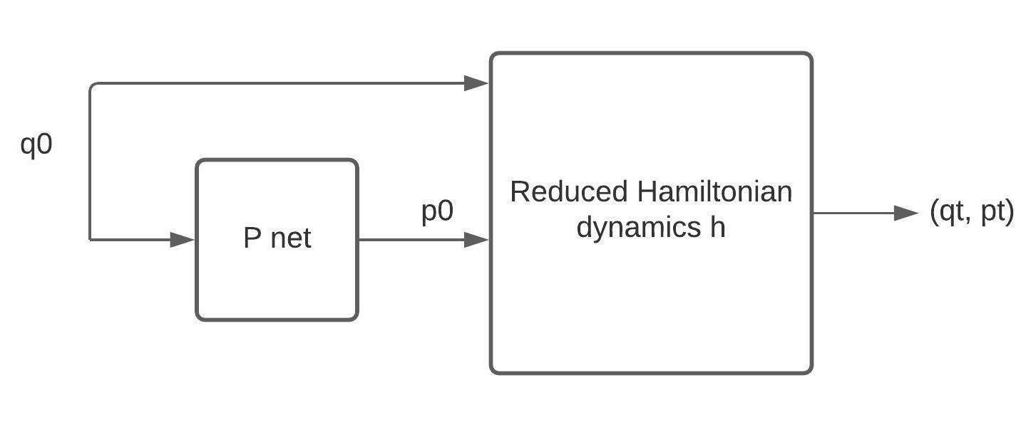
Training: As a first step, we start with the following training procedure called $\textit{AE}(T)$ for a fixed terminal time $T$:

1. Starting from $q_{0}$, we use $P$-net to obtain $p_{0}$

2. Now given $(q_{0},p_{0})$, run reduced Hamiltonian dynamics specified by $h_{\theta}$ to obtain $(q_{T},p_{T})$

3. Minimize the loss function $\mathcal{L}=\mathcal{L}(\theta,\phi)$:

   $$\begin{split}&\mathcal{L}(\theta,\phi)=\alpha_{1}\lVert p_{0}-\nabla g(q_{0})\rVert^{2}\\ &+\alpha_{2}\lVert p_{T}-\nabla g(q_{T})\rVert^{2}+\\ &\beta\lVert h_{\theta}(q_{0},p_{0})-(\langle p_{0},\hat{f}(q_{0},\hat{u}_{0})\rangle+l(q_{0},\hat{u}_{0}))\rVert^{2}\end{split}$$ (13)

   where $\alpha_{1}$, $\alpha_{2}$ and $\beta$ are hyperparameters, and $\hat{u}_{0}=-f_{u}(q_{0})^{T}p_{0}$. Here $\hat{f}(q_{0},\hat{u}_{0})$ can be either $f(q_{0},\hat{u}_{0})$ or $\partial_{p}h(q(0),p(0))$. We provide access to black-boxes of $f$, $g$, and/or $f_{u}$.

3.3 Second phase of variational training

Given the result of our first training procedure $\textit{AE}(T)$, we now have an additional variational training that encodes $(q_{0},p_{0})$ to $(q_{t},p_{t})$. The distribution of $(q_{t},p_{t})$ is simpler that that of $(q_{0},p_{0})$ as optimal state $q_{t}$ may concentrate on a few states while $p_{t}$ is close to $\nabla g(q_{t})$. This motivates us to build a variational autoencoder to further learn better the relation between starting state $x=(q_{0},p_{0})$, which can have complex distribution, and the final optimal state $y=(q_{t},p_{t})$. We further encode $(q_{t},p_{t})$ into a latent variable $z$, where we can impose simple prior distribution such as Gaussian. In this setting, we have the following 3 neural networks: encoder and decoder for latent variable $z$, and a Hamiltonian dynamics network $h_{\theta_{1}}$ that serves as the decoder from $y=(q_{t},p_{t})$ to $x=(q_{0},p_{0})$. The encoder $h_{\theta}$ is already built from the previous phase. Now the training process is similar to that of VAE and we wish to optimize the loss function $\mathcal{L}=\mathcal{L}(\theta_{1})$:

$$\begin{split}\mathcal{L}(\theta_{1})&=\alpha_{1}(KL(Q(z|y)||P(z))\\ &+\alpha_{2}\lVert x-\hat{x}\rVert^{2}+\lVert y-\hat{y}\rVert^{2}\end{split}$$ (14)

where $P$ and $Q$ are the prior and posterior distributions of the latent variable $z$, and $\alpha_{1}$ and $\alpha_{2}$ are two hyperparameters. Note that the decoder to $(q_{0},p_{0})$ is based on the backward ODE with dynamics function $(-h_{\theta_{1}})$. We call this VAE training process $\textit{VAE}(T)$ for the terminal time $T$.

Figure 2: Network architecture for phase 2

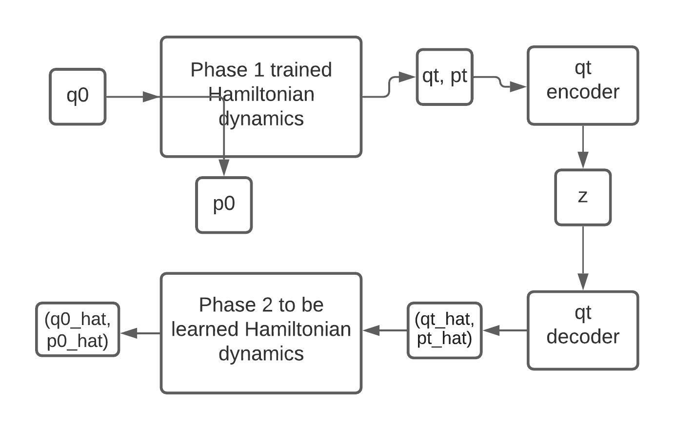
In summary, our training process for a variational learning of the reduced Hamiltonian includes:

• Phase 1: Run the first training procedure $\textit{AE}(T_{1})$.

• Phase 2: Run the variational procedure $\textit{VAE}(T_{2})$.

4 Infinite dimensional case

For a specific infinite-dimensional version of the optimal control problem, the Pontryagin maximum principle still holds [14] and gives us a way to use the method we presented in section 3. More specifically, we apply the Hamiltonian dynamics training on a truncated subspace of the infinite-dimensional space and obtain an approximate optimal control solution after learning the corresponding Hamiltonian dynamics.

4.1 Optimal control on infinite-dimensional space

We consider the following specific infinite-dimensional state space $M$:

State space: The space $M$ is an open subset of a Banach space $X$, a space on which a group of diffeomorphisms $\textit{Diff}_{0}^{l}(\mathbb{R}^{d})$ act continuously, with the action $(\phi,q)\mapsto\phi\cdot q$. More details on the structure of the group of diffeomorphisms is in [15]. For simplicity, in this paper, we specifically consider $M$ to be the set of all mappings from $S$ to $\mathbb{R}^{d}$, for a fixed subset $S$ of $\mathbb{R}^{d}$, which can be either discrete or continuous.

We now give descriptions for all the components in an infinite-dimensional optimal control problem.

State: A state $q$ is simply an element of the state space $M$: $q$ is a map from $S$ to $\mathbb{R}^{d}$. For example, if $d=2$ and $S$ is $S^{1}$, then $q$ is a closed curve in the set of all possible simple closed curves. This type of state occurs in free-form shape optimization problems

Control: We control the the map from $S$ to $\mathbb{R}^{d}$ by a velocity vector-field $v:\mathbb{R}^{d}\to\mathbb{R}^{d}$, which dictates how the map is deformed into another map. More details are given in the dynamics specified below. Note that the control $v$ lies in the control space $V$, which is the Hilbert vector space of all vector fields on $\mathbb{R}^{d}$.

Continuous-time dynamics: $\dot{q}(t)=\xi_{q(t)}v(t)$. Here $\xi_{q}$ is the differential of the map $\phi\mapsto\phi\cdot q$, and $\phi\in\textit{Diff}_{0}^{l}(\mathbb{R}^{d})$, the space of diffeomorphisms that acts continuously on the state space $M$. Because $M$ is the set of all mappings from $S$ to $\mathbb{R}^{d}$, the dynamics is reduced to $\xi_{q}v=v\circ q$.

Cost for choosing control $u$ in state $x$: $l(q(t),u(t))$ for some loss function $l$. In this paper, we initially restrict our attention to the special case, where the running cost is kinetic energy: $l(q,v)=\frac{1}{2}\lVert v\rVert_{V}^{2}$.

Terminal cost function: Let $g:M\to\mathbb{R}$ be a functional on infinite-dimensional state space. Then terminal cost is $g(q(T))$ with terminal time $T$.

Cost functional: We want to minimize the following cost $J$:

$$J(q,v)=\int_{0}^{T}l(q(t),v(t))dt+g(q(T))$$ (15)

Given the above description, we can define the infinite-dimensional version of Hamiltonian $H:M\times X^{*}\times V\times Y^{*}\to\mathbb{R}$:

$$H(q,p,v)=\langle p,\xi_{q}v\rangle_{X^{*},X}+l(q,v)$$ (16)

where the inner-product is defined between an element of $X$ and an element of its dual space $X^{*}$. Then 1 still holds for this infinite-dimensional setting.

5 Experiments

5.1 Finite-dimensional case

5.1.1 Cart pole

We consider the classical control problem of balancing the pole on a cart. We developed a continuous version of this problem based on the OpenAI Gym suite [16] together with necessary black boxes. We then train the agent using the procedure $\textit{AE}(T_{1})$ (See fig. 3), and then perform an additional training procedure $\textit{VAE}(T_{2})$ (See fig. 5) for $T_{1}=T_{2}=1$. The agent’s performance is clearly better than the untrained version (See fig. 4). With an additional $\textit{VAE}(T_{2})$ training, the agent seems to be more active, and tries to move around while keeping the pole balanced.

(a) First snapshot

(b) Second snapshot

(c) Third snapshot

(d) Fourth snapshot

Figure 3: Snapshots of the optimal trajectory from $\textit{AE}(T_{1})$ for cart pole.

(a) First snapshot

(b) Second snapshot

(c) Third snapshot

(d) Fourth snapshot

Figure 4: Snapshots from a random trajectory for cart pole.

(a) First snapshot

(b) Second snapshot

(c) Third snapshot

(d) Fourth snapshot

Figure 5: Snapshots from optimal trajectory with both types of training.

5.1.2 Mountain car

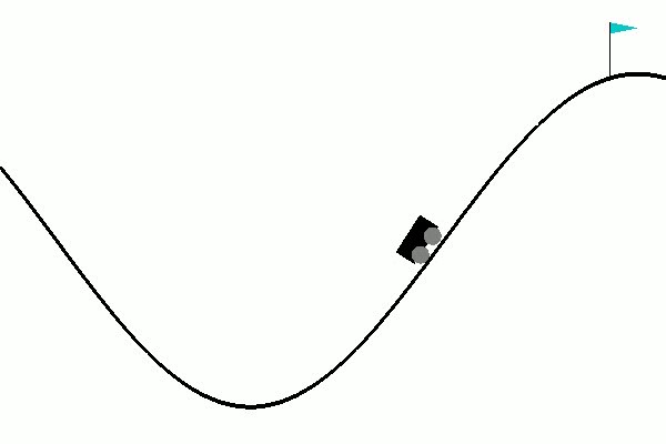
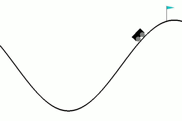
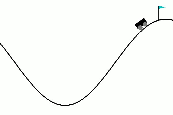
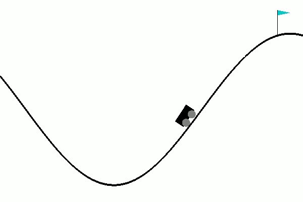
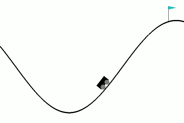
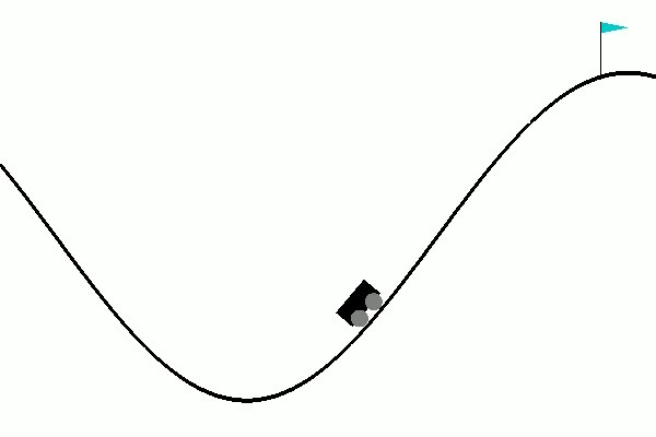
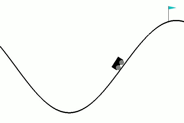
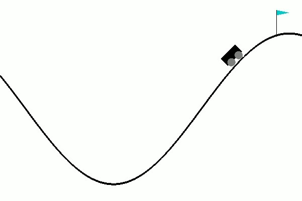
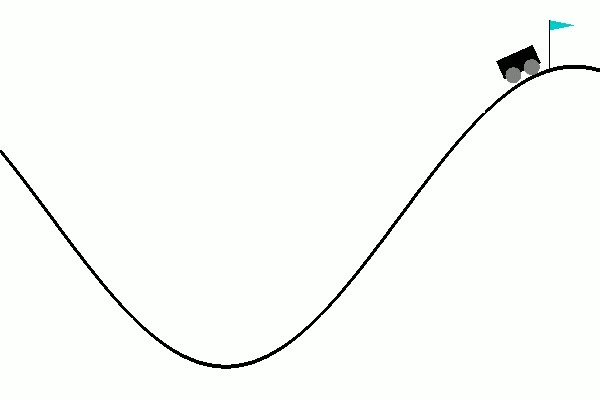
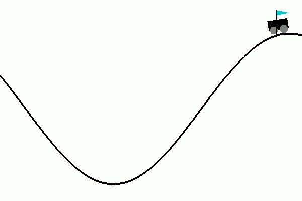
Next we consider the mountain car problem of controlling the force to move the car uphill. We use a similar setup for mountain car problem. Again we train the agent by using the procedure $\textit{AE}(T_{1})$ (See fig. 6). We then do an additional training pass with $\textit{VAE}(T_{2})$ (See fig. 8) for $T_{1}=T_{2}=1$. The agent’s performances in both types of trainings are clearly better than the untrained version (See fig. 7). In fact, for the untrained version, the car can only stay near the valley.

(a) First snapshot

(b) Second snapshot

(c) Third snapshot

(d) Fourth snapshot

Figure 6: Snapshots of the optimal trajectory from $\textit{AE}(T_{1})$ for mountain car.

(a) First snapshot

(b) Second snapshot

(c) Third snapshot

(d) Fourth snapshot

Figure 7: Snapshots from a random trajectory for mountain car.

(a) First snapshot

(b) Second snapshot

(c) Third snapshot

(d) Fourth snapshot

Figure 8: Snapshots from optimal trajectory with both types of training.

5.2 Infinite-dimensional case: Shape optimization

In this infinite-dimensional case, we consider optimizing a functional on the class of shapes. We restrict our problem to 2D setting. In the simplest form, a shape can be represented as a 2D density function. The formal formulation is presented in section 4. Here in the experiment, we choose the following functional $\mathcal{F}$ for the minimization problem:

$$\mathcal{F}(S)=\frac{\textit{Peri}(S)}{\sqrt{\textit{Area}(S)}},\text{ for shape }S$$ (17)

If $S$ can be decomposed into distinct connected components, then $\textit{Peri}(S)$ is defined to be the absolute value of the sum of signed areas of those connected components. The same definition applies for $\textit{Area}(S)$ but with area instead. The optimal shape $S$ in this problem is the one that has constant positive curvature $1$.

For this experiment, we put each shape $S$ in a 2D square. Everything in the shape has white color while everything outside is black (See fig. 9, fig. 10, and fig. 11). We discretize the shape by using 16 dimensions and spline interpolation. We train the agent with $\textit{AE}(T_{1})$ and $\textit{VAE}(T_{2})$ for $T_{1}=T_{2}=1$.

The trained agent with only $\textit{AE}(T_{1})$ training (See fig. 9) attempts to flatten out the region with negative curvature by closing the hole in the upper left corner. Similarly, the agent with additional $\textit{VAE}(T_{2})$ training tries to flatten out the negative curvature part in the lower right corner of the larger connected component (See fig. 11). On the other hand, the untrained agent doesn’t have any specific movement (See fig. 10) that helps to minimize the functional cost.

(a) First snapshot

(b) Second snapshot

(c) Third snapshot

(d) Fourth snapshot

Figure 9: Snapshots of the optimal trajectory from $\textit{AE}(T_{1})$ for shape optimization.

(a) First snapshot

(b) Second snapshot

(c) Third snapshot

(d) Fourth snapshot

Figure 10: Snapshots from a random trajectory for shape optimization

(a) First snapshot

(b) Second snapshot

(c) Third snapshot

(d) Fourth snapshot

Figure 11: Snapshots from optimal trajectory with both types of training.

6 Conclusion

In this paper, we build a continuous stochastic framework to learn the solution of optimal control problems with both finite and infinite-dimensional phase (state) spaces. By using the Pontryagin maximum principle, we reduce the problem to a specific kind of Hamiltonian dynamical system learning. The control is now encoded into the adjoint variable, and the new task is to learn this adjoint variable as well as the reduced Hamiltonian. This is fundamentally different from reinforcement learning, which focuses on action and value functions. We present two training procedures: one is static and is based on Pontryagin maximum principle’s conditions, and the other is variational inference. This framework allows us to further improve our work with appropriate state sample-efficient learning schemes [17]. Our future plans also includes improved network training processes with hyper-parameter optimization, and applying them to new types of stochastic control problems. We aim additionally to provide theoretical convergence bounds for our training procedures, and further develop our framework and its stochastic counterpart to become sophisticated alternatives to current reinforcement learning practice.

Acknowledgement: The research was supported in part by NIH-R01GM117594, by the Peter O’Donnell Foundation, and in part from a grant from the Army Research Office accomplished under Cooperative Agreement Number W911NF-19-2-0333.

Appendix A Network architectures

We report the network architectures used in training phase 1 and phase 2 for 3 types of problems correponding to three different environments considered in the experiments: cart pole, mountain car and shape optimization (optimizing on 2D density maps). For phase 1, we report dimension of state $q$, the dimensions of all hidden layers of the adjoint network $P_{\phi}$, and of the Hamiltonian network $h_{\theta}$.

Table 1: Network architecture for phase 1 training

Environment	State dimension	Adjoint network	Hamiltonian network
Cart pole	4	[16, 32, 32]	[16, 32, 64, 8]
Mountain car	2	[8, 16, 32]	[8, 16, 32]
Shape optimization	16	[32, 64]	[64, 8]

For phase 2, we report the dimension of latent variable $z$, the dimensions of all hidden layers of Hamiltonian decoder $h_{\theta_{1}}$, the dimensions of all hidden layers of the encoder from $y=(q_{t},p_{t})$ to the latent variable $z$, and of the decoder from the latent variable $z$ to $y=(q_{t},p_{t})$.

Table 2: Network architecture for phase 2 training

Environment	Latent dimension	Hamiltonian decoder	Decoder layer
Cart pole	4	[16, 32, 64, 8]	[16, 64]
Mountain car	2	[8, 16, 32]	[8, 32]
Shape optimization	4	[64, 8]	[8, 16, 64]

Encoder share layer	Encoder mean layer	Encoder log variance layer
[64]	[16]	[16]
[32]	[8]	[8]
[64]	[16, 8]	[16, 8]

Appendix B Details of the running cost (Lagrangian) and dynamics functions used in the experiments

B.1 Classical controls

For classical controls experiments including mountain car and cartpole, we choose the dynamics similar to the one given in the OpenAI Gym suite [16]. The states for these two problems are:

1. Mountain car: state $q=(x,\dot{x})$, where $x$ and $\dot{x}$ are position and velocity of the car.

2. Cart pole: state $q=(x,\dot{x},\theta,\dot{\theta})$, where $x$ and $\dot{x}$ are position and velocity of the cart, while $\theta$ and $\dot{\theta}$ are angle and angular velocity of the pole with respect to the cart.

We choose $l_{1}(q)$ component for the running cost $l(q,v)$ as follows:

1. Mountain car: $l_{1}(q)=(x-x_{0})^{2}+(\dot{x}-\dot{x}_{0})^{2}$, where $x_{0}$ and $\dot{x}_{0}$ are the goal position and velocity.

2. Cart pole: $l_{1}(q)=\theta^{2}$, as we don’t want the pole to deviate too much from the vertical line.

B.2 Shape optimization

The shape is quantified by its level-set function and the dynamics comes from the level-set equation. The control is simply the velocity of the deformation of the shape, and the $l_{1}(q)$ portion of a shape $q$ is exactly $\mathcal{F}(q)$, where the functional cost $\mathcal{F}$ on shapes is specified above.

Appendix C Details of other supplementary files

We include in the supplementary materials the videos of the optimal trajectories output by the models trained with phase 1 and phase 2 training, and also a random trajectory when the models are not trained. All videos are put in the videos folder and include the following files:

1. Cart pole

   • test_cartpole.wmv: trajectory output by models trained with only phase 1.

   • test_cartpole_phase2.wmv: trajectory output by models trained with both phase 1 and 2.

   • test_cartpole_untrained.wmv: random trajectory output by untrained models.

2. Mountain car

   • test_mountain_car.wmv: trajectory output by models trained with only phase 1.

   • test_mountain_car_phase2.wmv: trajectory output by models trained with both phase 1 and 2.

   • test_mountain_car_untrained.wmv: random trajectory output by untrained models.

3. Shape optimization

   • test_shape_opt.wmv: trajectory output by models trained with only phase 1.

   • test_shape_opt_phase2.wmv: trajectory output by models trained with both phase 1 and 2.

   • test_shape_opt_untrained.wmv: random trajectory output by untrained models.

All videos have WMV format. Finally, we don’t include the code in the supplementary materials. The code is instead available at https://cvc-lab.github.io/cvc-website/projects/optimal-control.

References

- [1] Emanuel Todorov. Optimal control theory. In Bayesian Brain, Doya, K. (ed), pages 1–28. MIT Press (2006), 12 2006.
- [2] LS Pontryagin, VG Boltyanskiy, RV Gamkrelidze, and YE Mischenko. Mathematical theory of optimal processes. John Wiley & Sons, 1962.
- [3] Amanda Lampton, Adam Niksch, and John Valasek. Reinforcement learning of a morphing airfoil-policy and discrete learning analysis. J. Aerosp. Comput. Inf. Commun., 7(8):241–260, 2010.
- [4] Jonathan Viquerat, Jean Rabault, Alexander Kuhnle, Hassan Ghraieb, Aurélien Larcher, and Elie Hachem. Direct shape optimization through deep reinforcement learning. Journal of Computational Physics, 428:110080, 2021.
- [5] Pieter Abbeel, Morgan Quigley, and Andrew Y Ng. Using inaccurate models in reinforcement learning. In Proceedings of the 23rd international conference on Machine learning, pages 1–8, 2006.
- [6] Sergey Levine and Pieter Abbeel. Learning neural network policies with guided policy search under unknown dynamics. In NIPS, volume 27, pages 1071–1079. Citeseer, 2014.
- [7] Marc Deisenroth and Carl E Rasmussen. Pilco: A model-based and data-efficient approach to policy search. In Proceedings of the 28th International Conference on machine learning (ICML-11), pages 465–472. Citeseer, 2011.
- [8] Nicolas Heess, Gregory Wayne, David Silver, Timothy Lillicrap, Tom Erez, and Yuval Tassa. Learning continuous control policies by stochastic value gradients. In C. Cortes, N. Lawrence, D. Lee, M. Sugiyama, and R. Garnett, editors, Advances in Neural Information Processing Systems, volume 28. Curran Associates, Inc., 2015.
- [9] Volodymyr Mnih, Koray Kavukcuoglu, David Silver, Andrei A Rusu, Joel Veness, Marc G Bellemare, Alex Graves, Martin Riedmiller, Andreas K Fidjeland, Georg Ostrovski, et al. Human-level control through deep reinforcement learning. nature, 518(7540):529–533, 2015.
- [10] Michael Lutter, Christian Ritter, and Jan Peters. Deep lagrangian networks: Using physics as model prior for deep learning. CoRR, abs/1907.04490, 2019.
- [11] Shixiang Gu, Timothy Lillicrap, Ilya Sutskever, and Sergey Levine. Continuous deep q-learning with model-based acceleration. In International conference on machine learning, pages 2829–2838. PMLR, 2016.
- [12] Guy Bouchitté and Giuseppe Buttazzo. Characterization of optimal shapes and masses through monge-kantorovich equation. Journal of the European Mathematical Society, 3(2):139–168, 2001.
- [13] Donald E Kirk. Optimal Control Theory: An Introduction. Prentice-Hall, London, England, 1971.
- [14] Sylvain Arguillère, Emmanuel Trélat, Alain Trouvé, and Laurent Younes. Shape deformation analysis from the optimal control viewpoint. J. Math. Pures Appl., 104(1):139–178, 2015.
- [15] Sylvain Arguillère and Emmanuel Trélat. Sub-Riemannian structures on groups of diffeomorphisms. J. Inst. Math. Jussieu, 16(4):745–785, 2017.
- [16] Greg Brockman, Vicki Cheung, Ludwig Pettersson, Jonas Schneider, John Schulman, Jie Tang, and Wojciech Zaremba. Openai gym, 2016.
- [17] Charles Gadd, Markus Heinonen, Harri Lähdesmäki, and Samuel Kaski. Sample-efficient reinforcement learning using deep gaussian processes, 2020.