Best of Both Worlds: Practical and Theoretically Optimal Submodular Maximization in Parallel

Abstract

For the problem of maximizing a monotone, submodular function with respect to a cardinality constraint $k$ on a ground set of size $n$, we provide an algorithm that achieves the state-of-the-art in both its empirical performance and its theoretical properties, in terms of adaptive complexity, query complexity, and approximation ratio; that is, it obtains, with high probability, query complexity of $O\left(n\right)$ in expectation, adaptivity of $O\left(\log(n)\right)$, and approximation ratio of nearly $1-1/e$. The main algorithm is assembled from two components which may be of independent interest. The first component of our algorithm, LinearSeq, is useful as a preprocessing algorithm to improve the query complexity of many algorithms. Moreover, a variant of LinearSeq is shown to have adaptive complexity of $O(\log(n/k))$ which is smaller than that of any previous algorithm in the literature. The second component is a parallelizable thresholding procedure ThresholdSeq for adding elements with gain above a constant threshold. Finally, we demonstrate that our main algorithm empirically outperforms, in terms of runtime, adaptive rounds, total queries, and objective values, the previous state-of-the-art algorithm FAST in a comprehensive evaluation with six submodular objective functions.

1 Introduction

The cardinality-constrained optimization of a monotone, submodular function $f:2^{\mathcal{N}}\to\mathbb{R}^{+}$, defined on subsets of a ground set $\mathcal{N}$ of size $n$, is a general problem formulation that is ubiquitous in wide-ranging applications, e.g. video or image summarization [30], network monitoring [26], information gathering [23], and MAP Inference for Determinantal Point Processes [20], among many others. The function $f:2^{\mathcal{N}}\to\mathbb{R}^{+}$ is submodular iff for all $S\subseteq T\subseteq\mathcal{N}$, $x\not\in T$, $\Delta\left(x\,|\,T\right)\leq\Delta\left(x\,|\,S\right)$; and the function $f$ is monotone if $f(S)\leq f(T)$ for all $S\subseteq T$. In this paper, we study the following submodular maximization problem (SM)

$$\text{maximize}f(S),\text{ subject to }|S|\leq k,$$ (SM)

where $f$ is a monotone, submodular function; SM is an NP-hard problem. There has been extensive effort into the design of approximation algorithms for SM over the course of more than 45 years, e.g. [32, 12, 10, 21, 24]. For SM, the optimal ratio has been shown to be $1-1/e\approx 0.63$ [32].

As instance sizes have grown very large, there has been much effort into the design of efficient, parallelizable algorithms for SM. Since queries to the objective function can be very expensive, the overall efficiency of an algorithm for SM is typically measured by the query complexity, or number of calls made to the objective function $f$ [2, 9]. The degree of parallelizability can be measured by the adaptive complexity of an algorithm, which is the minimum number of rounds into which the queries to $f$ may be organized, such that within each round, the queries are independent and hence may be arbitrariliy parallelized. Observe that the lower the adaptive complexity, the more parallelizable an algorithm is. To obtain a constant approximation factor, a lower bound of $\Omega(n)$ has been shown on the query complexity [24] and a lower bound of $\Omega(\log(n)/\log\log(n))$ has been shown on the adaptive complexity [3].

Several algorithms have been developed recently that are nearly optimal in terms of query and adaptive complexities [14, 11, 17, 5]; that is, these algorithms achieve $O\left(\log n\right)$ adaptivity and $O\left(n\text{polylog}(n)\right)$ query complexity (see Table 1). However, these algorithms use sampling techniques that result in very large constant factors that make these algorithms impractical. This fact is discussed in detail in Breuer et al. [9]; as an illustration, to obtain ratio $1-1/e-0.1$ with 95% confidence, all of these algorithms require more than $10^{6}$ queries of sets of size $k/\log(n)$ in every adaptive round [9]; moreover, even if these algorithms are run as heuristics using a single sample, other inefficiencies preclude these algorithms of running even on moderately sized instances [9]. For this reason, the FAST algorithm of Breuer et al. [9] has been recently proposed, which uses an entirely different sampling technique called adaptive sequencing. Adaptive sequencing was originally introduced in Balkanski et al. [6], but the original version has quadratic query complexity in the size of the ground set and hence is still impractical on large instances. To speed it up, the FAST algorithm sacrifices theoretical guarantees to yield an algorithm that parallelizes well and is faster than all previous algorithms for SM in an extensive experimental evaluation. The theoretical sacrifices of FAST include: the adaptivity of FAST is $\Omega(\log(n)\log^{2}(\log n))$, which is higher than the state-of-the-art, and more significantly, the algorithm obtains no approximation ratio for $k<850$; since many applications require small choices for $k$, this limits the practical utility of FAST. A natural question is thus: is it possible to design an algorithm that is both practical and theoretically optimal in terms of adaptivity, ratio, and total queries?

1.1 Contributions

Table 1: Theoretical comparison to algorithms that achieve nearly optimal adaptivity, ratio, and query complexity: the algorithm of Ene and Nguyen [14], randomized-parallel-greedy (RPG) of Chekuri and Quanrud [11], Binary-Search-Maximization (BSM) and Subsample-Maximization (SM) of Fahrbach et al. [17], FAST of Breuer et al. [9]. The symbol $\dagger$ indicates the result holds with constant probability or in expectation; the symbol $\ddagger$ indicates the result does not hold on all instances of SM; while no symbol indicates the result holds with probability greater than $1-O(1/n)$. Observe that our algorithm LS+PGB dominates in at least one category when compared head-to-head with any one of the previous algorithms.

Reference	Ratio	Adaptivity	Queries
Ene and Nguyen [14]	$1-1/e-\varepsilon$	$O\left(\frac{1}{\varepsilon^{2}}\log(n)\right)$	$O\left(n\text{poly}(\log n,1/\varepsilon)\right)$
Chekuri and Quanrud [11] (RPG)	$1-1/e-\varepsilon$	$O\left(\frac{1}{\varepsilon^{2}}\log(n)\right)\,\dagger$	$O\left(\frac{n}{\varepsilon^{4}}\log(n)\right)\,\dagger$
Fahrbach et al. [17] (BSM)	$1-1/e-\varepsilon\,\dagger$	$O\left(\frac{1}{\varepsilon^{2}}\log\left(n\right)\right)$	$O\left(\frac{n}{\varepsilon^{3}}\log\log k\right)\,\dagger$
Fahrbach et al. [17] (SM)	$1-1/e-\varepsilon\,\dagger$	$O\left(\frac{1}{\varepsilon^{2}}\log\left(n\right)\right)$	$O\left(\frac{n}{\varepsilon^{3}}\log(1/\varepsilon)\right)\,\dagger$
Breuer et al. [9] (FAST)	$1-1/e-\varepsilon\,\ddagger$	$O\left(\frac{1}{\varepsilon^{2}}\log(n)\log^{2}\left(\frac{\log(k)}{\varepsilon}\right)\right)$	$O\left(\frac{n}{\varepsilon^{2}}\log\left(\frac{\log(k)}{\varepsilon}\right)\right)$
LS+PGB [Theorem 3]	$1-1/e-\varepsilon$	$O\left(\frac{1}{\varepsilon^{2}}\log\left(n/\varepsilon\right)\right)$	$O\left(\frac{n}{\varepsilon^{2}}\right)\,\dagger$

Table 2: Empirical comparison of our algorithm with FAST, with each algorithm using 75 CPU threads on a broad range of $k$ values and six applications; details provided in Section 4. Parameter settings are favorable to FAST, which is run without theoretical guarantees while LS+PGB enforces ratio $\approx 0.53$ with high probability. For each application, we report the arithmetic mean of each metric over all instances. Observe that LS+PGB outperforms FAST in runtime on all applications.

	Runtime (s)		Objective Value		Queries
Application	FAST	LS+PGB	FAST	LS+PGB	FAST	LS+PGB
TrafficMonitor	$3.7\times 10^{-1}$	$\textbf{2.1}\times\textbf{10}^{\textbf{-1}}$	$4.7\times 10^{8}$	$\textbf{5.0}\times\textbf{10}^{\textbf{8}}$	$3.5\times 10^{3}$	$\textbf{2.4}\times\textbf{10}^{\textbf{3}}$
InfluenceMax	$4.4\times 10^{0}$	$\textbf{2.3}\times\textbf{10}^{\textbf{0}}$	$1.1\times 10^{3}$	$1.1\times 10^{3}$	$7.7\times 10^{4}$	$\textbf{4.0}\times\textbf{10}^{\textbf{4}}$
TwitterSumm	$1.6\times 10^{1}$	$\textbf{3.5}\times\textbf{10}^{\textbf{0}}$	$3.8\times 10^{5}$	$3.8\times 10^{5}$	$1.5\times 10^{5}$	$\textbf{6.2}\times\textbf{10}^{\textbf{4}}$
RevenueMax	$3.9\times 10^{2}$	$\textbf{5.4}\times\textbf{10}^{\textbf{1}}$	$1.4\times 10^{4}$	$1.4\times 10^{4}$	$7.6\times 10^{4}$	$\textbf{2.7}\times\textbf{10}^{\textbf{4}}$
MaxCover (BA)	$3.7\times 10^{2}$	$\textbf{7.6}\times\textbf{10}^{\textbf{1}}$	$6.0\times 10^{4}$	$\textbf{6.3}\times\textbf{10}^{\textbf{4}}$	$5.8\times 10^{5}$	$\textbf{1.8}\times\textbf{10}^{\textbf{5}}$
ImageSumm	$1.6\times 10^{1}$	$\textbf{8.1}\times\textbf{10}^{\textbf{-1}}$	$9.1\times 10^{3}$	$9.1\times 10^{3}$	$1.3\times 10^{5}$	$\textbf{4.8}\times\textbf{10}^{\textbf{4}}$

In this paper, we provide three main contributions. The first contribution is the algorithm LinearSeq (LS, Section 2) that achieves with probability $1-1/n$ a constant factor $(4+O(\varepsilon))^{-1}$ in expected linear query complexity and with $O(\log n)$ adaptive rounds (Theorem 1). Although the ratio of $\approx 0.25$ is smaller than the optimal $1-1/e\approx 0.63$, this algorithm can be used to improve the query complexity of many extant algorithms, as we decribe in the related work section below. Interestingly, LinearSeq can be modified to have adaptivity $O\left(\log(n/k)\right)$ at a small cost to its ratio as discussed in Appendix F. This version of LinearSeq is a constant-factor algorithm for SM with smaller adaptivity than any previous algorithm in the literature, especially for values of $k$ that are large relative to $n$.

Our second contribution is an improved parallelizable thresholding procedure ThresholdSeq (TS, Section 3) for a commonly recurring task in submodular optimization: namely, add all elements that have a gain of a specified threshold $\tau$ to the solution. This subproblem arises not only in SM, but also e.g. in submodular cover [17] and non-monotone submodular maximization [4, 18, 15, 25]. Our TS accomplishes this task with probability $1-1/n$ in $O(\log n)$ adaptive rounds and expected $O(n)$ query complexity (Theorem 2), while previous procedures for this task only add elements with an expected gain of $\tau$ and use expensive sampling techniques [17]; have $\Omega(\log^{2}n)$ adaptivity [22]; or have $\Omega(kn)$ query complexity [6].

Finally, we present in Section 3 the parallelized greedy algorithm ParallelGreedyBoost (PGB), which is used in conjunction with LinearSeq and ThresholdSeq to yield the final algorithm LS+PGB, which answers the above question affirmatively: LS+PGB obtains nearly the optimal $1-1/e$ ratio with probability $1-2/n$ in $O(\log n)$ adaptive rounds and $O(n)$ queries in expectation; moreover, LS+PGB is faster than FAST in an extensive empirical evaluation (see Table 2). In addition, LS+PGB improves theoretically on the previous algorithms in query complexity while obtaining nearly optimal adaptivity (see Table 1).

1.2 Additional Related Work

Adaptive Sequencing. The main inefficiency of the adaptive sequencing method of Balkanski et al. [6] (which causes the quadratic query complexity) is an explicit check that a constant fraction of elements will be filtered from the ground set. In this work, we adopt a similar sampling technique to adaptive sequencing, except that we design the algorithm to filter a constant fraction of elements with only constant probability. This method allows us to reduce the quadratic query complexity of adaptive sequencing to linear query complexity while only increasing the adaptive complexity by a small constant factor. In contrast, FAST of Breuer et al. [9] speeds up adaptive sequencing by increasing the adaptive complexity of the algorithm through adaptive binary search procedures, which, in addition to the increasing the adaptivity by logarithmic factors, place restrictions on the $k$ values for which the ratio can hold. This improved adaptive sequencing technique is the core of our ThresholdSeq procedure, which has the additional benefit of being relatively simple to analyze.

Algorithms with Linear Query Complexity. Our LinearSeq algorithm also uses the improved adaptive sequencing technique, but in addition this algorithm integrates ideas from the $\Omega(n)$-adaptive linear-time streaming algorithm of Kuhnle [24] to achieve a constant-factor algorithm with low adaptivity in expected linear time. Integration of the improved adaptive sequencing with the ideas of Kuhnle [24] is non-trivial, and ultimately this integration enables the theoretical improvement in query complexity over previous algorithms with sublinear adaptivity that obtain a constant ratio with high probability (see Table 1). In Fahrbach et al. [17], a linear-time procedure SubsamplePreprocessing is described; this procedure is to the best of our knowledge the only algorithm in the literature that obtains a constant ratio with sublinear adaptive rounds and linear query complexity and hence is comparable to LinearSeq. However, SubsamplePreprocessing uses entirely different ideas from our LinearSeq and has much weaker theoretical guarantees: for input $0<\delta<1$, it obtains ratio $\frac{\delta^{2}}{2\times 10^{6}}$ with probability $1-\delta$ in $O(\log(n)/\delta)$ adaptive rounds and $O(n)$ queries in expectation – the small ratio renders SubsamplePreprocessing impractical; also, its ratio holds only with constant probability. By contrast, with $\varepsilon=0.1$, our LinearSeq obtains ratio $\approx 0.196$ with probability $1-1/n$ in $O(\log(n))$ adaptive rounds and $O(n)$ queries in expectation.

Using LS for Preprocessing: Guesses of OPT. Many algorithms for SM, including FAST and all of the algorithms listed in Table 1 except for SM and our algorithm, use a strategy of guessing logarithmically many values of OPT. Our LinearSeq algorithm reduces the interval containing OPT from size $k$ to a small constant size in expected linear time. Thus, LinearSeq could be used for preprocessing prior to running FAST or one of the other algorithms in Table 1, which would improve their query complexity without compromising their adaptive complexity or ratio; this illustrates the general utility of LinearSeq. For example, with this change, the theoretical adaptivity of FAST improves, although it remains worse than LS+PGB: the adaptive complexity of FAST becomes $O\left(\frac{1}{\varepsilon^{2}}\log(n)\log\left(\frac{1}{\varepsilon}\log(k)\right)\right)$ in contrast to the $O\left(\frac{1}{\varepsilon^{2}}\log\left(n/\varepsilon\right)\right)$ of LS+PGB. Although SubsamplePreprocessing may be used for the same purpose, its ratio only holds with constant probability which would then limit the probability of success of any following algorithm.

Relationship of ThresholdSeq to Existing Methods. The first procedure in the literature to perform the same task is the ThresholdSampling procedure of Fahrbach et al. [17]; however, ThresholdSampling only ensures that the expected marginal gain of each element added is at least $\tau$ and has large constants in its runtime that make it impractical [9]. In contrast, ThresholdSeq ensures that added elements contribute a gain of at least $\tau$ with high probability and is highly efficient empirically. A second procedure in the literature to perform the same task is the Adaptive-Sequencing method of Balkanski et al. [6], which similarly to ThresholdSeq uses random permutations of the ground set; however, Adaptive-Sequencing focuses on explicitly ensuring a constant fraction of elements will be filtered in the next round, which is expensive to check: the query complexity of Adaptive-Sequencing is $O(kn)$. In contrast, our ThresholdSeq algorithm ensures this property with a constant probability, which is sufficient to ensure the adaptivity with the high probability of $1-1/n$ in $O(n)$ expected queries. Finally, a third related procedure in the literature is ThresholdSampling of Kazemi et al. [22], which also uses random permutations to sample elements. However, this algorithm has the higher adaptivity of $O\left(\log(n)\log(k)\right)$, in contrast to the $O\left(\log(n)\right)$ of ThresholdSeq.

MapReduce Framework. Another line of work studying parallelizable algorithms for SM has focused on the MapReduce framework [13] in a distributed setting, e.g. [7, 8, 16, 28]. These algorithms divide the dataset over a large number of machines and are intended for a setting in which the data does not fit on a single machine. None of these algorithms has sublinear adaptivity and hence all have potentially large numbers of sequential function queries on each machine. In this work, our empirical evaluation is on a single machine with a large number of CPU cores; we do not evaluate our algorithms in a distributed setting.

Organization. The constant-factor algorithm LinearSeq is described and analyzed in Section 2; the details of the analysis are presented in Appendix C. The variant of LinearSeq with lower adaptivity is described in Appendix F. The algorithms ThresholdSeq and ParallelGreedyBoost are discussed at a high level in Section 3, with detailed descriptions of these algorithms and theoretical analysis presented in Appendices D and E. Our empirical evaluation is summarized in Section 4 with more results and discussion in Appendix H.

2 A Parallelizable Algorithm with Linear Query Complexity: LinearSeq

Algorithm 1 The algorithm that obtains ratio $(4+O\left(\varepsilon)\right)^{-1}$ in $O\left(\log(n)/\varepsilon^{3}\right)$ adaptive rounds and expected $O\left(n/\varepsilon^{3}\right)$ queries.

1:procedure LinearSeq($f,\mathcal{N},k,\varepsilon$)

2:     Input: evaluation oracle $f:2^{\mathcal{N}}\to\mathbb{R}^{+}$, constraint $k$, error $\varepsilon$

3:     $a=\arg\max_{u\in\mathcal{N}}f(\{u\})$

4:     Initialize $A\leftarrow\{a\}$ , $V\leftarrow\mathcal{N}$, $\ell=\lceil 4(1+1/(\beta\varepsilon))\log(n)\rceil$, $\beta=\varepsilon/(16\log(8/(1-e^{-\varepsilon/2})))$

5:     for  $j\leftarrow 1$ to $\ell$  do

6:         Update $V\leftarrow\{x\in V:\Delta\left(x\,|\,A\right)\geq f(A)/k\}$ and filter out the rest

7:         if $|V|=0$ then break

8:         $V=\{v_{1},v_{2},\ldots,v_{|V|}\}\leftarrow$random-permutation$(V)$

9:         $\Lambda\leftarrow\{\lfloor(1+\varepsilon)^{u}\rfloor:1\leq\lfloor(1+\varepsilon)^{u}\rfloor\leq k,u\in\mathbb{N}\}$

10:$\qquad\qquad\qquad\cup\{\lfloor k+u\varepsilon k\rfloor:\lfloor k+u\varepsilon k\rfloor\leq|V|,u\in\mathbb{N}\}\cup\{|V|\}$

11:         $B[\lambda_{i}]=\textbf{false}$, for $\lambda_{i}\in\Lambda$

12:         for $\lambda_{i}\in\Lambda$ in parallel  do

13:              $T_{\lambda_{i-1}}\leftarrow\{v_{1},v_{2},\ldots,v_{\lambda_{i-1}}\}$ ; $T_{\lambda_{i}}\leftarrow\{v_{1},v_{2},\ldots,v_{\lambda_{i}}\}$ ; $T_{\lambda_{i}}^{\prime}\leftarrow T_{\lambda_{i}}\backslash T_{\lambda_{i-1}}$

14:              if $\Delta\left(T_{\lambda_{i}}^{\prime}\,|\,A\cup T_{\lambda_{i-1}}\right)/|T_{\lambda_{i}}^{\prime}|\geq(1-\varepsilon)f(A\cup T_{\lambda_{i-1}})/k$ then $B[\lambda_{i}]\leftarrow\textbf{true}$          

15:         $\lambda^{*}\leftarrow\max\{\lambda_{i}\in\Lambda:B[\lambda_{i}]=\textbf{false}$ and $\left((\lambda_{i}\leq k\text{ and }B[1]\text{ to }B[\lambda_{i-1}]\text{ are all }\textbf{true})\right.$ or $(\lambda_{i}>k\text{ and }\exists m\geq 1\text{ s.t. }|\bigcup_{u=m}^{i-1}T_{\lambda_{u}}^{\prime}|\geq k$ and $B[\lambda_{m}]\text{ to }B[\lambda_{i-1}]\text{ are all }\textbf{true}))\}$

16:         $A\leftarrow A\cup T_{\lambda^{*}}$      

17:     if $|V|>0$ then return failure

18:     return $A^{\prime}\leftarrow$ last $k$ elements added to $A$

In this section, we describe the algorithm LinearSeq for SM (Alg. 1) that obtains ratio $(4+O\left(\varepsilon\right))^{-1}$ in $O\left(\frac{1}{\varepsilon^{3}}\log(n)\right)$ adaptive rounds and expected $O\left(\frac{n}{\varepsilon^{3}}\right)$ queries. If $\varepsilon\leq 0.21$, the ratio of LinearSeq is lower-bounded by $(4+16\varepsilon)^{-1}\geq 0.135$, which shows that a relatively large constant ratio is obtained even at large values of $\varepsilon$. An initial run of this algorithm is required for our main algorithm LS+PGB.

Description of LS. The work of LS is done within iterations of a sequential outer for loop (Line 5); this loop iterates at most $O\left(\log(n)\right)$ times, and each iteration requires two adaptive rounds; thus, the adaptive complexity of the algorithm is $O\left(\log(n)\right)$. Each iteration adds more elements to the set $A$, which is initially empty. Within each iteration, there are four high-level steps: 1) filter elements from $V$ that have gain less than $f(A)/k$ (Line 6); 2) randomly permute $V$ (Line 8); 3) compute in parallel the marginal gain of adding blocks of the sequence of remaining elements in $V$ to $A$ (for loop on Line 12); 4) select a prefix of the sequence $V=\left(v_{1},v_{2},\ldots,v_{|V|}\right)$ to add to $A$ (Line 15). The selection of the prefix to add is carefully chosen to approximately satisfy, on average, Condition 1 for elements added; and also to ensure that, with constant probability, a constant fraction of elements of $V$ are filtered on the next iteration.

The following theorem states the theoretical results for LinearSeq. The remainder of this section proves this theorem, with intuition and discussion of the proof. The omitted proofs for all lemmata are provided in Appendix C.

Theorem 1.

Let $(f,k)$ be an instance of SM. For any constant $0<\varepsilon<1/2$, the algorithm LinearSeq has adaptive complexity $O\left(\log(n)/\varepsilon^{3}\right)$ and outputs $A^{\prime}\subseteq\mathcal{N}$ with $|A^{\prime}|\leq k$ such that the following properties hold: 1) The algorithm succeeds with probability at least $1-1/n$. 2) There are $O\left((1/(\varepsilon k)+1)n/\varepsilon^{3}\right)$ oracle queries in expectation. 3) If the algorithm succeeds, $\left[4+\frac{4(2-\varepsilon)}{(1-\varepsilon)(1-2\varepsilon)}\varepsilon\right]f(A^{\prime})\geq f(O)$, where $O$ is an optimal solution to the instance $(f,k)$.

Overview. The goal of this section is to produce a constant factor, parallelizable algorithm with linear query complexity. As a starting point, consider an algorithm that takes one pass through the ground set, adding each element $e$ to candidate set $A$ iff

$$\Delta\left(e\,|\,A\right)\geq f(A)/k.$$ (1)

Condition 1 ensures two properties: 1) the last $k$ elements in $A$ contain a constant fraction of the value $f(A)$; and 2) $f(A)$ is within a constant fraction of OPT. By these two properties, the last $k$ elements of $A$ are a constant factor approximation to SM with exactly one query of the objective function per element of the ground set. For completeness, we give a pseudocode (Alg. 3) and proof in Appendix B. However, each query depends on all of the previous ones and thus there are $n$ adaptive rounds. Therefore, the challenge is to approximately simulate Alg. 3 in a lowly adaptive (highly parallelizable) manner, which is what LinearSeq accomplishes.

2.1 Approximately Satisfying Condition 1

Discarding Elements. In one adaptive round during each iteration $j$ of the outer for loop, all elements with gain to $A$ of less than $f\left(A\right)/k$ are discarded from $V$ (Line 6). Since the size of $A$ increases as the algorithm runs, by submodularity, the gain of these elements can only decrease and hence these elements cannot satisfy Condition 1 and can be safely discarded from consideration. The process of filtering thereby ensures the following lemma at termination.

Lemma 1.

At successful termination of LinearSeq, $f(O)\leq 2f(A)$, where $O\subseteq\mathcal{N}$ is an optimal solution of size $k$.

Addition of Elements. Next, we describe the details of how elements are added to the set $A$. The random permutation of remaining elements on Line 8 constructs a sequence $\left(v_{1},v_{2},\ldots,v_{|V|}\right)$ such that each element is uniformly randomly sampled from the remaining elements. By testing the marginal gains along the sequence in parallel, it is possible to determine a good prefix of the sequence $(v_{i})$ to add to $A$ to ensure the following: 1) Condition 1 is approximately satisfied; and 2) We will discard a constant fraction of $V$ in the next iteration with constant probability. Condition 1 is important for the approximation ratio and discarding a constant fraction of $V$ is important for the adaptivity and query complexity. Below, we discuss how to choose the prefix such that both are achieved. To speed up the algorithm, we do not test the marginal gain at each point in the sequence $(v_{i})$, but rather test blocks of elements at once as determined by the index set $\Lambda$ defined in the pseudocode.

Prefix Selection. Say a block is bad if this block does not satisfy the condition checked on Line 14 (which is an approximate, average form of Condition 1); otherwise, the block is good. At the end of an iteration, we select the largest block index $\lambda^{*}$, where this block is bad and the previous consecutive blocks which together have at least $k$ elements are all good; or this block is bad and all the previous blocks are good blocks. Then, we add the prefix $T_{\lambda^{*}}=(v_{1},v_{2},\ldots,v_{\lambda^{*}})$ into $A$. Now, the relevance of Condition 1 for the approximation ratio is that it implies $f(A)\geq 2f(A\setminus A^{\prime})$, where $A^{\prime}$ are the last $k$ elements added to $A$. Lemma 2 shows that the conditions required on the marginal gains of blocks added imply an approximate form of this fact is satisfied by LinearSeq. Indeed, the proof of Lemma 2 informs the choice $\Lambda$ of blocks evaluated and the computation of $\lambda^{*}$.

Lemma 2.

Suppose LinearSeq terminates successfully. Then $f(A)\geq\frac{2(1-\varepsilon+\varepsilon^{2})}{1+\varepsilon}f(A\backslash A^{\prime})$.

Proof.

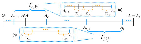
Figure 1: This figure depicts the way elements are added to $A$, with $A_{i}$ denoting the value of $A$ after iteration $i$ of the outer for loop; the prefix added at iteration $i$ is denoted by $T_{i,\lambda_{i}^{*}}$. The orange lines mark the blocks comprising each prefix. Also, the set $A^{\prime}$ of the last $k$ elements added to $A$ is shown. Parts (a) and (b) depict two separate cases in the proof of Claim 1.

If $|A|\leq k$, the lemma is immediate, so assume $|A|>k$. For iteration $j$, let $T_{j,\lambda_{j}^{*}}$ denote the set added to $A$ during iteration $j$; and let $T_{j,\lambda_{j}^{*}}=\emptyset$ if the algorithm terminates before iteration $j$. Let $A_{j}$ denote the value of $A$ after iteration $j$. Define $c=\max\{c\in\mathbb{N}:A^{\prime}\subseteq(\cup_{j=c}^{\ell}T_{j,\lambda_{j}^{*}})\}$. Then, $|T_{c,\lambda_{c}^{*}}|>0$; and for any $j>c$, $|T_{j,\lambda_{j}^{*}}|<k$. It holds that $(\cup_{j=c+1}^{\ell}T_{j,\lambda_{j}^{*}})\subset A^{\prime}\subseteq(\cup_{j=c}^{\ell}T_{j,\lambda_{j}^{*}})$. Figure 1 shows how $A$ is composed of these sets $T_{j,\lambda_{j}^{*}}$ and how each set is composed of blocks. The following claim is proven in Appendix C.3.

Claim 1.

It holds that $\Delta\left(T_{c,\lambda_{c}^{*}}\,|\,A\backslash A^{\prime}\right)\geq(1-\varepsilon)\max\{0,|T_{c,\lambda_{c}^{*}}\cap A^{\prime}|-2\varepsilon k\}\cdot f(A\backslash A^{\prime})/k.$ For $j>c$, it holds that $\Delta\left(T_{j,\lambda_{j}^{*}}\,|\,A_{j-1}\right)\geq\frac{1-\varepsilon}{1+\varepsilon}|T_{j,\lambda_{j}^{*}}|\cdot f(A\backslash A^{\prime})/k.$

From Claim 1,

$$f(A)-f(A\backslash A^{\prime})=\Delta\left(T_{c,\lambda_{c}^{*}}\,|\,A\backslash A^{\prime}\right)+\sum_{j=c+1}^{\ell}\Delta\left(T_{j,\lambda_{j}^{*}}\,|\,A_{j-1}\right)\geq\frac{(1-\varepsilon)(1-2\varepsilon)}{1+\varepsilon}\cdot f(A\backslash A^{\prime}),$$ (2)

where Inequality 2 is proven in Appendix C.4. ∎

In the remainder of this subsection, we will show that a $(\beta\varepsilon)$-fraction of $V$ is discarded at each iteration $j$ of the outer for loop with probability at least $1/2$, where $\beta$ is a constant in terms of $\varepsilon$ as defined on Line 4 in the pseudocode. The remainder of the proofs in this section are implicitly conditioned on the behavior of the algorithm prior to iteration $j$. The next lemma describes the behavior of the number of elements that will be filtered at iteration $j+1$. Observe that the set $S_{i}$ defined in the next lemma is the set of elements that would be filtered at the next iteration if prefix $T_{i}$ is added to $A$.

Lemma 3.

Let $S_{i}=\left\{x\in V:\Delta\left(x\,|\,A\cup T_{i}\right)<f(A\cup T_{i})/k\right\}.$ It holds that $|S_{0}|=0$, $|S_{|V|}|=|V|$, and $|S_{i}|\leq|S_{i+1}|$.

By Lemma 3, we know the number of elements in $S_{i}$ increases from 0 to $|V|$ with $i$. Therefore, there exists a $t$ such that $t=\min\{i\in\mathbb{N}:|S_{i}|\geq\beta\varepsilon|V|\}$. If $\lambda^{*}\geq t$, $|S_{\lambda^{*}}|\geq\beta\varepsilon|V|$, and we will successfully filter out more than $(\beta\varepsilon)$-fraction of $V$ at the next iteration. In this case, we say that the iteration $j$ succeeds. Otherwise, if $\lambda^{*}<t$, the iteration may fail. The remainder of the proof bounds the probability that $\lambda^{*}<t$, which is an upper bound on the probability that iteration $j$ fails. Let $\lambda_{t}=\max\{\lambda\in\Lambda:\lambda<t\}$, and let $\lambda_{t}^{\prime}=\max(\{\lambda^{\prime}\in\Lambda:\sum_{\lambda\in\Lambda,\lambda^{\prime}\leq\lambda\leq\lambda_{t}}|T_{\lambda}|\geq k\}\cup\{1\})$. If $\lambda^{*}<t$, there must be at least one index $\lambda$ between $\lambda_{t}^{\prime}$ and $\lambda_{t}$ such that the block $T^{\prime}_{\lambda}$ is bad. The next lemma bounds the probability that any block $T_{\lambda}^{\prime},$ with $\lambda<\lambda_{t}$, is bad.

Lemma 4.

Let $t=\min\{i\in\mathbb{N}:|S_{i}|\geq\beta\varepsilon|V|\}$; $\lambda_{t}=\max\{\lambda\in\Lambda:\lambda<t\}$; $(Y_{i})$ be a sequence of independent and identically distributed Bernoulli trials, where the success probability is $\beta\varepsilon$. Then for any $\lambda<\lambda_{t}$, $Pr\left(B[\lambda]=\textbf{false}\right)\leq Pr\left(\sum_{i=1}^{|T^{\prime}_{\lambda}|}Y_{i}>\varepsilon|T^{\prime}_{\lambda}|\right)$.

Finally, we bound the probability that an iteration $j$ of the outer for loop fails. Let $B_{1}=\{\lambda\in\Lambda:\lambda\leq k\text{ and }\lambda<\lambda_{t}\}$, $B_{2}=\{\lambda\in\Lambda:|\Lambda\cap[\lambda,\lambda_{t}]|\leq\lceil 1/\varepsilon\rceil\}$. Then

$$Pr\left(\text{iteration $j$ fails}\right)\leq Pr\left(\exists\lambda\in B_{1}\cup B_{2}\text{ with }B[\lambda]=\textbf{false}\right)\leq 1/2,$$ (3)

where the proof of Inequality 3 is in Appendix C.7.

2.2 Proof of Theorem 1

From Section 2.1, the probability at any iteration of the outer for loop of successful filtering of an $(\beta\varepsilon)$-fraction of $V$ is at least $1/2$. We can model the success of the iterations as a sequence of dependent Bernoulli random variables, with success probability that depends on the results of previous trials but is always at least $1/2$.

Success Probability of LinearSeq. If there are at least $m=\lceil\log_{1-\beta\varepsilon}(1/n)\rceil$ successful iterations, the algorithm LinearSeq will succeed. The number of successful iterations $X_{\ell}$ up to and including the $\ell$-th iteration is a sum of dependent Bernoulli random variables. With some work (Lemma 6 in Appendix A), the Chernoff bounds can be applied to ensure the algorithm succeeds with probability at least $1-1/n$, as shown in Appendix C.2.

Adaptivity and Query Complexity. Oracle queries are made on Lines 6 and 14 of LinearSeq. The filtering on Line 6 is in one adaptive round, and the inner for loop is also in one adaptive round. Thus, the adaptivity is proportional to the number of iterations of the outer for loop, $O\left(\ell\right)=O\left(\log(n)/\varepsilon^{3}\right).$ For the query complexity, let $Y_{i}$ be the number of iterations between the $(i-1)$-th and $i$-th successful iterations of the outer for loop. By Lemma 6 in Appendix A, $\mathbb{E}\left[Y_{i}\right]\leq 2$. From here, we show in Appendix C.8 that there are at most $O\left(n/\varepsilon^{3}\right)$ queries in expectation.

Approximation Ratio. Suppose LinearSeq terminates successfully. We have the approximation ratio as follows:

$$f(A^{\prime})\overset{(a)}{\geq}f(A)-f(A\backslash A^{\prime})\overset{(b)}{\geq}f(A)-\frac{1+\varepsilon}{2(1-\varepsilon+\varepsilon^{2})}f(A)\overset{(c)}{\geq}\frac{1}{4+\frac{4(2-\varepsilon)}{(1-\varepsilon)(1-2\varepsilon)}\cdot\varepsilon}f(O),$$

where Inequality (a) is from submodularity of $f$, Inequality (b) is from Lemma 2, and Inequality (c) is from Lemma 1.

3 Improving to Nearly the Optimal Ratio

In this section, we describe how to obtain the nearly optimal ratio in nearly optimal query and adaptive complexities (Section 3.2). First, in Section 3.1, we describe ThresholdSeq, a parallelizable procedure to add all elements with gain above a constant threshold to the solution. In Section 3.2, we describe ParallelGreedyBoost and finally the main algorithm LS+PGB. Because of space constraints, the algorithms are described in the main text at a high level only, with detailed descriptions and proofs deferred to Appendices D and E.

3.1 The ThresholdSeq Procedure

In this section, we discuss the algorithm ThresholdSeq, which adds all elements with gain above an input threshold $\tau$ up to accuracy $\varepsilon$ in $O(\log n)$ adaptive rounds and $O(n)$ queries in expectation. Pseudocode is given in Alg. 4 in Appendix D.

Overview. The goal of this algorithm is, given an input threshold $\tau$ and size constraint $k$, to produce a set of size at most $k$ such that the average gain of elements added is at least $\tau$. As discussed in Section 1, this task is an important subroutine of many algorithms for submodular optimization (including our final algorithm), although by itself it does not produce any approximation ratio for SM. The overall strategy of our parallelizable algorithm ThresholdSeq is analagous to that of LinearSeq, although ThresholdSeq is considerably simpler to analyze. The following theorem summarizes the theoretical guarantees of ThresholdSeq and the proofs are in Appendix D.

Theorem 2.

Suppose ThresholdSeq is run with input $(f,k,\varepsilon,\delta,\tau)$. Then, the algorithm has adaptive complexity $O(\log(n/\delta)/\varepsilon)$ and outputs $A\subseteq\mathcal{N}$ with $|A|\leq k$ such that the following properties hold: 1) The algorithm succeeds with probability at least $1-\delta/n$. 2) There are $O(n/\varepsilon)$ oracle queries in expectation. 3) It holds that $f(A)/|A|\geq(1-\varepsilon)\tau/(1+\varepsilon)$. 4) If $|A|<k$, then $\Delta\left(x\,|\,A\right)<\tau$ for all $x\in\mathcal{N}$.

3.2 The ParallelGreedyBoost Procedure and the Main Algorithm

Algorithm 2 The ParallelGreedyBoost procedure.

1:Input: evaluation oracle $f:2^{\mathcal{N}}\to\mathbb{R}^{+}$, constraint $k$, constant $\alpha$, value $\Gamma$ such that $\Gamma\leq f(O)\leq\Gamma/\alpha$, accuracy parameter $\varepsilon$

2:Initialize $\tau$ $\leftarrow$ $\Gamma/(\alpha k)$, $\delta$ $\leftarrow$ $1/(\log_{1-\varepsilon}(\alpha/3)+1)$, $A\leftarrow\emptyset$

3:while $\tau\geq\Gamma/(3k)$ do

4:     $\tau\leftarrow\tau(1-\varepsilon)$

5:     $S\leftarrow\textsc{ThresholdSeq}(f_{A},\mathcal{N},k-|A|,\delta,\varepsilon/3,\tau)$

6:     $A\leftarrow A\cup S$

7:     if $|A|=k$ then

8:         return $A$      

9:return A

In this section, we describe the greedy algorithm ParallelGreedyBoost (PGB, Alg. 2) that uses multiple calls to ThresholdSeq with descending thresholds. Next, our state-of-the-art algorithm LS+PGB is specified.

Description of ParallelGreedyBoost. This procedure takes as input the results from running an $\alpha$-approximation algorithm on the instance $(f,k)$ of SM; thus, ParallelGreedyBoost is not meant to be used as a standalone algorithm. Namely, ParallelGreedyBoost takes as input $\Gamma$, the solution value of an $\alpha$-approximation algorithm for SM; this solution value $\Gamma$ is then boosted to ensure the ratio $1-1/e-\varepsilon$ on the instance. The values of $\Gamma$ and $\alpha$ are used to produce an initial threshold value $\tau$ for ThresholdSeq. Then, the threshold value is iteratively decreased by a factor of $(1-\varepsilon)$ and the call to ThresholdSeq is iteratively repeated to build up a solution, until a minimum value for the threshold of $\Gamma/(3k)$ is reached. Therefore, ThresholdSeq is called at most $O\left(\log(1/\alpha)/\varepsilon\right)$ times. We remark that $\alpha$ is not required to be a constant approximation ratio.

Theorem 3.

Let $(f,k)$ be an instance of SM. Suppose an $\alpha$- approximation algorithm for SM is used to obtain $\Gamma$, where the approximation ratio $\alpha$ holds with probability $1-p_{\alpha}$. For any constant $\varepsilon>0$, the algorithm ParallelGreedyBoost has adaptive complexity $O\left(\frac{\log{\alpha^{-1}}}{\varepsilon^{2}}\log\left(\frac{n\log\left(\alpha^{-1}\right)}{\varepsilon}\right)\right)$ and outputs $A\in\mathcal{N}$ with $|A|\leq k$ such that the following properties hold: 1) The algorithm succeeds with probability at least $1-1/n-p_{\alpha}$. 2) If the algorithm succeeds, there are $O\left(n\log\left(\alpha^{-1}\right)/\varepsilon^{2}\right)$ oracle queries in expectation. 3) If the algorithm succeeds, $f(A)\geq(1-1/e-\varepsilon)f(O)$, where $O$ is an optimal solution to the instance $(f,k)$.

Proof.

Success Probability. For the while loop in Line 3-8, there are no more than $\lceil\log_{1-\varepsilon}(\alpha/3)\rceil$ iterations. If ThresholdSeq completes successfully at every iteration, Algorithm 2 also succeeds. The probability that this occurs is lower bounded in Appendix E.1.1. For the remainder of the proof of Theorem 3, we assume that every call to ThresholdSeq succeeds.

Adaptive and Query Complexity. There are at most $\lceil\log_{1-\varepsilon}(\alpha/3)\rceil$ iterations of the while loop. Since $\log(x)\leq x-1$, $\lceil\log_{1-\varepsilon}(\alpha/3)\rceil=\lceil\frac{\log(\alpha/3)}{\log(1-\varepsilon)}\rceil$, and $\varepsilon<1-1/e$, it holds that $\lceil\log_{1-\varepsilon}(\alpha/3)\rceil\leq\lceil\frac{\log(3/\alpha)}{\varepsilon}\rceil.$ And for each iteration, queries to the oracle happen only on Line 5, the call to ThresholdSeq. Since the adaptive and query complexity of ThresholdSeq is $O\left(\log(n/\delta)/\varepsilon\right)$ and $O\left(n/\varepsilon\right)$, the adaptive and query complexities for Algorithm 2 are $O\left(\frac{\log{\alpha^{-1}}}{\varepsilon^{2}}\log\left(\frac{n\log\left(\alpha^{-1}\right)}{\varepsilon}\right)\right),O\left(\frac{\log{\alpha^{-1}}}{\varepsilon^{2}}n\right),$ respectively.

Approximation Ratio. Let $A_{j}$ be the set $A$ we get after Line 6, and let $S_{j}$ be the set returned by ThresholdSeq in iteration $j$ of the while loop. Let $\ell$ be the number of iterations of the while loop.

First, in the case that $|A|<k$ at termination, ThresholdSeq returns $0\leq|S_{\ell}|<k-|A_{\ell-1}|$ at the last iteration. From Theorem 2, for any $o\in O$, $\Delta\left(o\,|\,A\right)<\tau<\Gamma/(3k)$. By submodularity and monotonicity, $f(O)-f(A)\leq f(O\cup A)-f(A)\leq\sum_{o\in O\backslash A}\Delta\left(o\,|\,A\right)\leq\sum_{o\in O\backslash A}\Gamma/(3k)\leq f(O)/3,$ and the ratio holds.

Second, consider the case that $|A|=k$. Suppose in iteration $j+1$, ThresholdSeq returns a nonempty set $S_{j+1}$. Then, in the previous iteration $j$, ThresholdSeq returns a set $S_{j}$ that $0\leq|S_{j}|<k-|A_{j-1}|$. From Theorem 2,

$$f(O)-f(A_{j+1})\leq\left(1-\frac{(1-\varepsilon/3)(1-\varepsilon)}{(1+\varepsilon/3)k}|A_{j+1}\backslash A_{j}|\right)(f(O)-f(A_{j})).$$ (4)

The above inequality also holds when $A_{j+1}=A_{j}$. Therefore, it holds that

$$f(O)-f(A)\leq e^{-\frac{(1-\varepsilon/3)(1-\varepsilon)}{1+\varepsilon/3}}f(O)\leq(1/e+\varepsilon)f(O).$$ (5)

The detailed proof of Inequality 4 and 5 can be found in Appendix E.1.2. ∎

Main Algorithm: LS+PGB. To obtain the main algorithm of this paper (and its nearly optimal theoretical guarantees), we use ParallelGreedyBoost with the solution value $\Gamma$ and ratio $\alpha$ given by LinearSeq. Because this choice requires an initial run of LinearSeq, we denote this algorithm by LS+PGB. Thus, LS+PGB integrates LinearSeq and ParallelGreedyBoost to get nearly the optimal $1-1/e$ ratio with query complexity of $O\left(n\right)$ and adaptivity of $O\left(\log(n)\right)$.

4 Empirical Evaluation

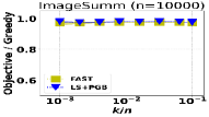
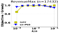
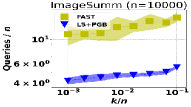
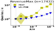
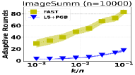
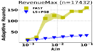
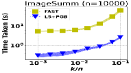
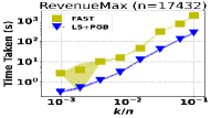
Figure 2: Evaluation of adaptive algorithms on ImageSumm and RevenueMax in terms of objective value normalized by the standard greedy value (Figure 2 - 2), total number of queries (Figure 2 - 2), total adaptive rounds (Figure 2 - 2) and the time required by each algorithm (Figure 2 - 2)

In this section, we demonstrate that the empirical performance of LS+PGB outperforms that of FAST for the metrics of total time, total queries, adaptive rounds, and objective value across six applications of SM: maximum cover on random graphs (MaxCover), twitter feed summarization (TweetSumm), image summarization (ImageSumm), influence maximization (Influence), revenue maximization (RevMax), and Traffic Speeding Sensor Placement (Traffic). See Appendix H.2 for the definition of the objectives. The sizes $n$ of the ground sets range from $n=1885$ to $100000$.

Implementation and Environment. We evaluate the same implementation of FAST used in Breuer et al. [9]. Our implementation of LS+PGB is parallelized using the Message Passing Interface (MPI) within the same Python codebase as FAST (see the Supplementary Material for source code). Practical optimizations to LinearSeq are made, which do not compromise the theoretical guarantees, which are discussed in Appendix G. The hardware of the system consists of 40 Intel(R) Xeon(R) Gold 5218R CPU @ 2.10GHz cores (with 80 threads available), of which up to 75 threads are made available to the algorithms for the experiments. On each instance, the algorithms are repeated independently for five repetitions, and the mean and standard deviation of the objective value, total queries, adaptive rounds and parallel (wall clock) runtime to the submodular function is plotted.

Parameters. The parameters $\varepsilon,\delta$ of FAST are set to enforce the nominal ratio of $1-1/e-0.1\approx 0.53$ with probability $0.95$; these are the same parameter settings for FAST as in the Breuer et al. [9] evaluation. The $\varepsilon$ parameter of LS+PGB is set to enforce the same ratio with probability $1-2/n$. With these parameters, FAST ensures its ratio only if $k\geq\theta(\varepsilon,\delta,k)=2\log(2\delta^{-1}\log(\frac{1}{\varepsilon}\log(k)))/\varepsilon^{2}(1-5\varepsilon)\geq 7103$. Since $k<7103$ on many of our instances, FAST is evaluated in these instances as a theoretically motivated heuristic. In contrast, the ratio of LS+PGB holds on all instances evaluated. We use exponentially increasing $k$ values from $n/1000$ to $n/10$ for each application to explore the behavior of each algorithm across a broad range of instance sizes.

Overview of Results. Figure 2 illustrates the comparison with FAST across the ImageSumm and RevenueMax application; results on other applications are shown in Appendix H. Runtime: LS+PGB is faster than FAST by more than $1\%$ on $80\%$ of instances evaluated; and is faster by an order of magnitude on $14\%$ of instances. Objective value: LS+PGB achieves higher objective by more than $1\%$ on $50\%$ of instances, whereas FAST achieves higher objective by more than $1\%$ on $8\%$ of instances. Adaptive rounds: LS+PGB achieves more than $1\%$ fewer adaptive rounds on $75\%$ of instances, while FAST achieves more than $1\%$ fewer adaptive rounds on $22\%$ of instances. Total queries: LS+PGB uses more than 1% fewer queries on $84\%$ of scenarios with FAST using more than 1% fewer queries on $9\%$ of scenarios. In summary, LS+PGB frequently gives substantial improvement in objective value, queries, adaptive rounds, and parallel runtime. Comparison of the arithmetic means of the metrics over all instances is given in Table 2. Finally, FAST and LS+PGB show very similar linear speedup with the number of processors employed: as shown in Fig. 7.

5 Concluding Remarks

In this work, we have introduced the algorithm LS+PGB, which is highly parallelizable and achieves state-of-the-art empirical performance over any previous algorithm for SM; also, LS+PGB is nearly optimal theoretically in terms of query complexity, adaptivity, and approximation ratio. An integral component of LS+PGB is our preprocessing algorithm LinearSeq, which reduces the interval containing OPT to a small constant size in expected linear time and low adaptivity, which may be independently useful. Another component of LS+PGB is the ThresholdSeq procedure, which adds all elements with gain above a threshold in a parallelizable manner and improves existing algorithms in the literature for the same task.

Appendix A Probability Lemma and Concentration Bounds

In this section, we state the Chernoff bound and prove a useful lemma (Lemma 6) for working with a sequence of dependent Bernoulli trials. Lemma 6 is applied in the analysis of both ThresholdSeq and LinearSeq.

Lemma 5.

(Chernoff bounds [31]). Suppose $X_{1}$, … , $X_{n}$ are independent binary random variables such that $Pr\left(X_{i}=1\right)=p_{i}$. Let $\mu=\sum_{i=1}^{n}p_{i}$, and $X=\sum_{i=1}^{n}X_{i}$. Then for any $\delta\geq 0$, we have

$$Pr\left(X\geq(1+\delta)\mu\right)\leq e^{-\frac{\delta^{2}\mu}{2+\delta}}.$$ (6)

Moreover, for any $0\leq\delta\leq 1$, we have

$$Pr\left(X\leq(1-\delta)\mu\right)\leq e^{-\frac{\delta^{2}\mu}{2}}.$$ (7)

Lemma 6.

Suppose there is a sequence of $n$ Bernoulli trials: $X_{1},X_{2},\ldots,X_{n},$ where the success probability of $X_{i}$ depends on the results of the preceding trials $X_{1},\ldots,X_{i-1}$. Suppose it holds that

$$Pr\left(X_{i}=1|X_{1}=x_{1},X_{2}=x_{2},\ldots,X_{i-1}=x_{i-1}\right)\geq\eta,$$

where $\eta>0$ is a constant and $x_{1},\ldots,x_{i-1}$ are arbitrary.

Then, if $Y_{1},\ldots,Y_{n}$ are independent Bernoulli trials, each with probability $\eta$ of success, then

$$Pr\left(\sum_{i=1}^{n}X_{i}\leq b\right)\leq Pr\left(\sum_{i=1}^{n}Y_{i}\leq b\right),$$

where $b$ is an arbitrary integer.

Moreover, let $A$ be the first occurrence of success in sequence $X_{i}$. Then,

$$\mathbb{E}\left[A\right]\leq 1/\eta.$$

Proof.

Let $Z_{j}=\sum_{i=1}^{j}X_{i}+\sum_{i=j+1}^{n}Y_{i}$, where $Z_{0}=\sum_{i=1}^{n}Y_{i}$ and $Z_{n}=\sum_{i=1}^{n}X_{i}$. Our goal is to prove that $Pr\left(Z_{n}\leq b\right)\leq Pr\left(Z_{0}\leq b\right)$. This lemma holds, if for any $j=1,\ldots,n$, $Pr\left(Z_{j}\leq b\right)\leq Pr\left(Z_{j-1}\leq b\right)$. With Bayes Theorem and Total Probability Theorem,

$$Pr\left(Z_{j}\leq b\right) =Pr\left(X_{j}=0,Z_{j}-X_{j}\leq b-1\right)+Pr\left(X_{j}=1,Z_{j}-X_{j}\leq b-1\right)$$

$$\quad+Pr\left(X_{j}=0,Z_{j}-X_{j}=b\right)$$

$$=Pr\left(Z_{j}-X_{j}\leq b-1\right)+\sum_{Z_{j}-X_{j}=b}Pr\left(X_{j}=0|X_{1},\ldots,X_{j-1},Y_{j+1},\ldots,Y_{n}\right)$$

$$\quad\cdot Pr\left(X_{1},\ldots,X_{j-1},Y_{j+1},\ldots,Y_{n}\right)$$

$$\leq Pr\left(Z_{j-1}-Y_{j}\leq b-1\right)$$

$$\quad+\sum_{Z_{j-1}-Y_{j}=b}Pr\left(Y_{j}=0\right)\cdot Pr\left(X_{1},\ldots,X_{j-1},Y_{j+1},\ldots,Y_{n}\right)$$ (8)

$$=Pr\left(Z_{j-1}-Y_{j}\leq b-1\right)+Pr\left(Y_{j}=0,Z_{j-1}-Y_{j}=b\right)$$

$$=Pr\left(Z_{j-1}\leq b\right),$$

where inequality 8 follows from $Pr\left(X_{j}=0|X_{1}=x_{1},X_{2}=x_{2},\ldots,X_{j-1}=x_{j-1}\right)\leq 1-\eta=Pr\left(Y_{j}=0\right)$ and $Z_{j}-X_{j}=Z_{j-1}-Y_{j}$.

Following the first inequality, we can prove the second one as follows:

$$\mathbb{E}\left[A\right] =\sum_{a\geq 1}aPr\left(A=a\right)$$

$$=\sum_{a\geq 1}aPr\left(X_{1}=\ldots=X_{a-1}=0,X_{a}=1\right)$$

$$=\sum_{a\geq 1}a\left(Pr\left(X_{1}=\ldots=X_{a-1}=0\right)-Pr\left(X_{1}=\ldots=X_{a}=0\right)\right)$$

$$=1+\sum_{a\geq 1}Pr\left(X_{1}=\ldots=X_{a}=0\right)$$

$$=1+\sum_{a\geq 1}Pr\left(\sum_{i=1}^{a}X_{a}\leq 0\right)$$

$$\leq 1+\sum_{a\geq 1}Pr\left(\sum_{i=1}^{a}Y_{a}\leq 0\right)$$

$$=1+\sum_{a\geq 1}Pr\left(Y_{1}=\ldots=Y_{a}=0\right)$$

$$=1+\sum_{a\geq 1}(1-\eta)^{a}$$

$$=1/\eta.$$

∎

Lemma 7.

Suppose there is a sequence of $n+1$ Bernoulli trials: $X_{1},X_{2},\ldots,X_{n+1},$ where the success probability of $X_{i}$ depends on the results of the preceding trials $X_{1},\ldots,X_{i-1}$, and it decreases from 1 to 0. Let $t$ be a random variable based on the $n+1$ Bernoulli trials. Suppose it holds that

$$Pr\left(X_{i}=1|X_{1}=x_{1},X_{2}=x_{2},\ldots,X_{i-1}=x_{i-1},i\leq t\right)\geq\eta,$$

where $x_{1},\ldots,x_{i-1}$ are arbitrary and $0<\eta<1$ is a constant. Then, if $Y_{1},\ldots,Y_{n+1}$ are independent Bernoulli trials, each with probability $\eta$ of success, then

$$Pr\left(\sum_{i=1}^{t}X_{i}\leq bt\right)\leq Pr\left(\sum_{i=1}^{t}Y_{i}\leq bt\right),$$

where $b$ is an arbitrary integer.

Proof.

Let $Z_{j}=\sum_{i=1}^{j}X_{i}\cdot 1_{\{i\leq t\}}+\sum_{i=j+1}^{n+1}Y_{i}\cdot 1_{\{i\leq t\}}$, where

$$Z_{0}=\sum_{i=1}^{n+1}Y_{i}\cdot 1_{\{i\leq t\}}=\sum_{i=1}^{t}Y_{i},$$

and

$$Z_{n+1}=\sum_{i=1}^{n+1}X_{i}\cdot 1_{\{i\leq t\}}=\sum_{i=1}^{t}X_{i}.$$

If for any $1\leq j\leq n+1$,

$$Pr\left(Z_{j}\leq bt\right)\leq Pr\left(Z_{j-1}\leq bt\right),$$ (9)

then,

$$Pr\left(Z_{n+1}\leq bt\right)\leq Pr\left(Z_{0}\leq bt\right).$$

We prove Inequality 9 as follows,

$$Pr\left(Z_{j}\leq bt\right)$$

$$=Pr\left(X_{j}\cdot 1_{\{j\leq t\}}=0,Z_{j}-X_{j}\cdot 1_{\{j\leq t\}}\leq bt-1\right)$$

$$\quad+Pr\left(X_{j}\cdot 1_{\{j\leq t\}}=1,Z_{j}-X_{j}\cdot 1_{\{j\leq t\}}\leq bt-1\right)$$

$$\quad+Pr\left(X_{j}\cdot 1_{\{j\leq t\}}=0,Z_{j}-X_{j}\cdot 1_{\{j\leq t\}}=bt\right)$$

$$=Pr\left(Z_{j}-X_{j}\cdot 1_{\{j\leq t\}}\leq bt-1\right)$$

$$\quad+Pr\left(1_{\{j\leq t\}}=0,Z_{j}-X_{j}\cdot 1_{\{j\leq t\}}=bt\right)$$

$$\quad+Pr\left(X_{j}=0,1_{\{j\leq t\}}=1,Z_{j}-X_{j}\cdot 1_{\{j\leq t\}}=bt\right)$$

$$=Pr\left(Z_{j}-X_{j}\cdot 1_{\{j\leq t\}}\leq bt-1\right)$$

$$\quad+Pr\left(1_{\{j\leq t\}}=0,Z_{j}-X_{j}\cdot 1_{\{j\leq t\}}=bt\right)$$

$$\quad+\sum_{Z_{j}-X_{j}\cdot 1_{\{j\leq t\}}=bt,j\leq t}Pr\left(X_{j}=0|X_{1},\cdots,X_{j-1},Y_{j+1},\cdots,Y_{n+1},j\leq t\right)$$

$$\quad\cdot Pr\left(X_{1},\cdots,X_{j-1},Y_{j+1},\cdots,Y_{n+1},j\leq t\right)$$

$$\leq Pr\left(Z_{j-1}-Y_{j}\cdot 1_{\{j\leq t\}}\leq bt-1\right)$$

$$\quad+Pr\left(1_{\{j\leq t\}}=0,Z_{j-1}-Y_{j}\cdot 1_{\{j\leq t\}}=bt\right)$$

$$\quad+\sum_{Z_{j-1}-Y_{j}\cdot 1_{\{j\leq t\}}=bt,j\leq t}Pr\left(Y_{j}=0\right)\cdot Pr\left(X_{1},\cdots,X_{j-1},Y_{j+1},\cdots,Y_{n+1},j\leq t\right)$$ (10)

$$=Pr\left(Z_{j-1}-Y_{j}\cdot 1_{\{j\leq t\}}\leq bt-1\right)$$

$$\quad+Pr\left(1_{\{j\leq t\}}=0,Z_{j-1}-Y_{j}\cdot 1_{\{j\leq t\}}=bt\right)$$

$$\quad+Pr\left(Y_{j}=0,1_{\{j\leq t\}}=1,Z_{j-1}-Y_{j}\cdot 1_{\{j\leq t\}}=bt\right)$$

$$=Pr\left(Z_{j-1}-Y_{j}\cdot 1_{\{j\leq t\}}\leq bt-1\right)$$

$$\quad+Pr\left(Y_{j}\cdot 1_{\{j\leq t\}}=0,Z_{j-1}-Y_{j}\cdot 1_{\{j\leq t\}}=bt\right)$$

$$=Pr\left(Z_{j-1}\leq bt\right),$$

where Inequality 10 follows from $Pr\left(X_{i}=1|X_{1}=x_{1},X_{2}=x_{2},\ldots,X_{i-1}=x_{i-1},i\leq t\right)\geq\eta$ and $Z_{j}-X_{j}\cdot 1_{\{j\leq t\}}=Z_{j-1}-Y_{j}\cdot 1_{\{j\leq t\}}$. ∎

Lemma 8.

(Wald’s Equation [34]). Let $(X_{n})_{n\in\mathbb{N}}$ be an infinite sequence of real-valued random variables and let $N$ be a nonnegative integer-valued random variable. Assume that: 1) $(X_{n})_{n\in\mathbb{N}}$ are all integrable (finite-mean) random variables, 2) $\mathrm{E}\left[X_{n}1_{\{N\geq n\}}\right]=\mathrm{E}\left[X_{n}\right]\mathrm{P}(N\geq n)$ for every natural number $n$, 3) the infinite series satisfies $\sum_{n=1}^{\infty}\mathrm{E}\left[\left|X_{n}\right|1_{\{N\geq n\}}\right]<\infty$. Then the random sums $S_{N}=\sum_{n=1}^{N}X_{n}$ and $T_{N}=\sum_{n=1}^{N}\mathrm{E}\left[X_{n}\right]$ are integrable and $\mathrm{E}\left[S_{N}\right]=\mathrm{E}\left[T_{N}\right]$.

Appendix B Highly Adaptive $0.25$-Approximation

In this section, we show that Alg. 3 achieves approximation ratio of $1/4$ in $n$ adaptive queries to the objective function $f$. Alg. 3 influences the design of LinearSeq, which uses similar ideas to obtain its constant ratio. See the discussion in Section 2.

Description of Alg. 3. This algorithm operates in one for loop through the ground set. Each element $u$ is added to a set $A$ iff. $\Delta\left(u\,|\,A\right)\geq f(A)/k$. The solution returned is the set $A^{\prime}$ of the last $k$ elements added to $A$.

Algorithm 3 Highly Adaptive Linear-Time Algorithm

1:Input: evaluation oracle $f:2^{\mathcal{N}}\to\mathbb{R}^{+}$, constraint $k$

2:Initialize $A\leftarrow\emptyset$

3:for  $u\in\mathcal{N}$  do

4:     if $\Delta\left(u\,|\,A\right)\geq f\left(A\right)/k$ then

5:         $A\leftarrow A\cup\{u\}$      

6:return $A^{\prime}\leftarrow\{\text{last }k\text{ elements added to }A\}$

Theorem 4.

Let $O$ be an optimal solution to SM on instance $(f,k)$. Then the set $A^{\prime}$ produced after running Alg. 3 on this instance satisfies $4f(A^{\prime})\geq f(O)$.

Proof.

Lemma 9.

At termination of Alg. 3, $f(O)\leq 2f(A)$.

Proof.

For each $o\in O\backslash A$, let $j(o)+1$ be the iteration of the for loop in which $o$ is processed, and $A_{j(o)}$ be $A$ after iteration $j(o)$. Thus, $\Delta\left(o\,|\,A_{j(o)}\right))<f(A_{j(o)})/k$. Then

$$f(O)-f(A) \leq f(O\cup A)-f(A)$$ (11)

$$\leq\sum_{o\in O\backslash A}\Delta\left(o\,|\,A\right)$$ (12)

$$\leq\sum_{o\in O\backslash A}\Delta\left(o\,|\,A_{j(o)}\right)$$ (13)

$$\leq\sum_{o\in O\backslash A}f(A_{j(o)})/k$$

$$\leq f(A),$$ (14)

where Inequalities 12 and 13 follow from submodularity, and Inequalities 11 and 14 follow from monotonicity. ∎

Lemma 10.

At termination of Alg. 3, $f(A)\leq 2f(A^{\prime})$.

Proof.

If $|A|<k$, then $A^{\prime}=A$ and there is nothing to show. So suppose $|A|\geq k$. Let $A^{\prime}_{i}=\{a_{1},\ldots,a_{i-1}\}$.

$$f(A)-f(A\setminus A^{\prime}) =\sum_{i=1}^{k}\Delta\left(a_{i}\,|\,A\setminus A^{\prime}\cup A^{\prime}_{i}\right)$$

$$\geq\sum_{i=1}^{k}f\left((A\setminus A^{\prime})\cup A^{\prime}_{i}\right)/k$$

$$\geq\sum_{i=1}^{k}f\left(A\setminus A^{\prime}\right)/k$$

$$=f\left(A\setminus A^{\prime}\right).$$

Therefore, $f\left(A\setminus A^{\prime}\right)\leq f(A)/2.$ Now,

$$f(A^{\prime}) \geq f(A)-f(A\setminus A^{\prime})$$ (15)

$$\geq f(A)-f(A)/2=f(A)/2,$$

where Inequality 15 is by submodularity of $f$. ∎

By Lemma 9 and 10, we have

$$f(O)\leq 2f(A)\leq 4f(A^{\prime}).$$

∎

Appendix C Analysis of LinearSeq

C.1 Proof of Lemma 1

See 1

Proof.

For each $o\in O\backslash A$, let $j(o)+1$ be the iteration where $o$ is filtered out, and $A_{j(o)}$ be $A$ after iteration $j(o)$. Thus, $\Delta\left(o\,|\,A_{j(o)}\right))<f(A_{j(o)})/k$. Then

$$f(O)-f(A) \leq f(O\cup A)-f(A)$$ (16)

$$\leq\sum_{o\in O\backslash A}\Delta\left(o\,|\,A\right)$$ (17)

$$\leq\sum_{o\in O\backslash A}\Delta\left(o\,|\,A_{j(o)}\right)$$ (18)

$$\leq\sum_{o\in O\backslash A}f(A_{j(o)})/k$$

$$\leq f(A),$$ (19)

where Inequalities 17 and 18 follow from submodularity, and Inequalities 16 and 19 follow from monotonicity. ∎

C.2 Probability LinearSeq is Successful

Proof.

Let $Y_{\ell}$ be the number of successes in $\ell$ independent Bernoulli random variables with success probability 1/2. Then,

$$Pr\left(\text{Algorithm \ref{alg:fastlinear} succeeds}\right) \geq Pr\left(Y_{\ell}\geq m\right)$$ (20)

$$\geq Pr\left(Y_{\ell}\geq\log(n)/(\beta\varepsilon)\right)$$

$$=1-Pr\left(Y_{\ell}\leq\log(n)/(\beta\varepsilon)\right)$$

$$\geq 1-e^{-\frac{1}{2}\left(\frac{2\beta\varepsilon+1}{2(\beta\varepsilon+1)}\right)^{2}\cdot 2\left(1+\frac{1}{\beta\varepsilon}\right)\log(n)}$$ (21)

$$=1-(\frac{1}{n})^{\frac{(2\beta\varepsilon+1)^{2}}{4\beta\varepsilon(\beta\varepsilon+1)}}$$

$$\geq 1-\frac{1}{n},$$

where Inequalities 20 and 21 follow from Lemma 6 and Lemma 5, respectively. ∎

C.3 Proof of Claim 1

See 1

Proof.

In this proof, let $T_{j,i}=(v_{1},\ldots,v_{i})$ be the prefix of $V$ of length $i$ at iteration $j$. Likewise, define $T^{\prime}_{j,i}=T_{j,i}\setminus T_{j,i-1}$. Say block $T_{j,k}^{\prime}$ is bad if this block does not satisfy the condition in Line 14 during iteration $j$.

First, consider the case that $j>c$. It holds that $T_{j,\lambda_{j}^{*}}\subseteq A^{\prime}$. Thus, $|T_{j,\lambda_{j}^{*}}|\leq k$. If $|T_{j,\lambda_{j}^{*}}|=0$, the result holds. If $0<|T_{j,\lambda_{j}^{*}}|\leq k$, then there are several blocks in $T_{j,\lambda_{j}^{*}}$, where the last one is bad and all the previous ones are good. Since the block size exponentially increases with ratio $1+\varepsilon$ when $\lambda_{i}\leq k$, it holds that $|T_{j,\lambda_{j}^{*}}^{\prime}|\leq\varepsilon/(1+\varepsilon)|T_{j,\lambda_{j}^{*}}|$. Then,

$$\Delta\left(T_{j,\lambda_{j}^{*}}\,|\,A_{j-1}\right) =\sum_{\lambda_{i}\leq\lambda_{j}^{*}}\Delta\left(T_{j,\lambda_{i}}^{\prime}\,|\,A_{j-1}\cup T_{j,\lambda_{i-1}}\right)$$

$$\geq\sum_{\lambda_{i}<\lambda_{j}^{*}}\Delta\left(T_{j,\lambda_{i}}^{\prime}\,|\,A_{j-1}\cup T_{j,\lambda_{i-1}}\right)$$ (22)

$$\geq\sum_{\lambda_{i}<\lambda_{j}^{*}}(1-\varepsilon)|T_{j,\lambda_{i}}^{\prime}|\cdot f(A_{j-1}\cup T_{j,\lambda_{i-1}})/k$$ (23)

$$\geq(1-\varepsilon)|T_{j,\lambda_{j}^{*}}\backslash T_{j,\lambda_{j}^{*}}^{\prime}|\cdot f(A\backslash A^{\prime})/k$$ (24)

$$\geq\frac{1-\varepsilon}{1+\varepsilon}|T_{j,\lambda_{j}^{*}}|\cdot f(A\backslash A^{\prime})/k,$$

where Inequalities 22 and 24 follow from monotonicity, and Inequality 23 follows from the property of good block.

Now consider the case $j=c$. In this case, block $T_{c,\lambda_{c}^{*}}^{\prime}$ is always a bad block. And, if $|T_{c,\lambda_{c}^{*}}|\leq k$, all the previous blocks are good; if $|T_{c,\lambda_{c}^{*}}|>k$, several previous blocks are good total with at least $k$ elements. Let $\lambda_{v}=\min\{\lambda_{v}\in\Lambda:\cup_{\lambda_{v}\leq\lambda_{i}\leq\lambda_{c}^{*}}T_{c,\lambda_{i}}^{\prime}\subseteq A^{\prime}\}$. Then, block $T_{c,\lambda_{v}}^{\prime}$ to the block before $T_{c,\lambda_{c}^{*}}^{\prime}$ are all good blocks. For any $\lambda_{i}\in\Lambda$, it holds that $|T_{c,\lambda_{i}}^{\prime}|\leq\varepsilon k$. Then,

$$\Delta\left(T_{c,\lambda_{c}^{*}}\,|\,A\backslash A^{\prime}\right) =\sum_{\lambda_{i}\leq\lambda_{c}^{*}}\Delta\left(T_{c,\lambda_{i}}^{\prime}\,|\,A\backslash A^{\prime}\cup T_{c,\lambda_{i-1}}\right)$$

$$\geq\sum_{\lambda_{v}\leq\lambda_{i}<\lambda_{c}^{*}}\Delta\left(T_{c,\lambda_{i}}^{\prime}\,|\,A\backslash A^{\prime}\cup T_{c,\lambda_{i-1}}\right)$$ (25)

$$\geq(1-\varepsilon)\sum_{\lambda_{v}\leq\lambda_{i}<\lambda_{c}^{*}}|T_{c,\lambda_{i}}^{\prime}|\cdot f(A\backslash A^{\prime}\cup T_{c,\lambda_{i-1}})/k$$ (26)

$$\geq(1-\varepsilon)\max\left\{0,\left(|T_{c,\lambda_{c}^{*}}\cap A^{\prime}|-|T_{c,\lambda_{v-1}}^{\prime}|-|T_{c,\lambda_{c}^{*}}^{\prime}|\right)\right\}\cdot f(A\backslash A^{\prime})/k$$ (27)

$$\geq(1-\varepsilon)\max\{0,|T_{c,\lambda_{c}^{*}}\cap A^{\prime}|-2\varepsilon k\}\cdot f(A\backslash A^{\prime})/k,$$

where Inequality 25 follows from monotonicity, Inequality 26 follows from the property of good block, Inequality 27 follows from monotonicity, $\cup_{\lambda_{v}\leq\lambda_{i}<\lambda_{c}^{*}}T_{c,\lambda_{i}}^{\prime}\subseteq\left(T_{c,\lambda_{c}^{*}}\cap A^{\prime}\right)$, and

$$\left(\left(T_{c,\lambda_{c}^{*}}\cap A^{\prime}\right)\backslash\cup_{u=v}^{i-1}T_{c,\lambda_{i}}^{\prime}\right)\subseteq\left(T_{c,\lambda_{v-1}}^{\prime}\cup T_{c,\lambda_{c}^{*}}^{\prime}\right).$$

∎

C.4 Proof of Inequality 2

Proof of Inequality 2.

$$f(A)-f(A\backslash A^{\prime})=\Delta\left(T_{c,\lambda_{c}^{*}}\,|\,A\backslash A^{\prime}\right)+\sum_{j=c+1}^{\ell}\Delta\left(T_{j,\lambda_{j}^{*}}\,|\,A_{j-1}\right)$$

$$\geq(1-\varepsilon)\max\{0,|T_{c,\lambda_{c}^{*}}\cap A^{\prime}|-2\varepsilon k\}\cdot f(A\backslash A^{\prime})/k+\frac{1-\varepsilon}{1+\varepsilon}\left(k-|T_{c,\lambda_{c}^{*}}\cap A^{\prime}|\right)\cdot f(A\backslash A^{\prime})/k$$

$$=(1-\varepsilon)\left(\max\left\{2\varepsilon-\frac{|T_{c,\lambda_{c}^{*}}\cap A^{\prime}|}{(1+\varepsilon)k},\frac{\varepsilon|T_{c,\lambda_{c}^{*}}\cap A^{\prime}|}{(1+\varepsilon)k}\right\}+\frac{1}{1+\varepsilon}-2\varepsilon\right)\cdot f(A\backslash A^{\prime})$$

$$\geq\frac{(1-\varepsilon)(1-2\varepsilon)}{1+\varepsilon}\cdot f(A\backslash A^{\prime})$$ (28)

where Inequality 28 follows from the fact that $\max\left\{2\varepsilon-\frac{|T_{c,\lambda_{c}^{*}}\cap A^{\prime}|}{(1+\varepsilon)k},\frac{\varepsilon|T_{c,\lambda_{c}^{*}}\cap A^{\prime}|}{(1+\varepsilon)k}\right\}\geq 2\varepsilon^{2}/(1+\varepsilon).$ ∎

C.5 Proof of Lemma 3

See 3

Proof.

After Line 6, for any $x\in V$, $\Delta\left(x\,|\,A\right)\geq f(A)/k$, $\Delta\left(x\,|\,V\cup A\right)=0$. Since $T_{0}=\emptyset$ and $T_{|V|}=V$,

$$|S_{0}| = |\{x\in V:\Delta\left(x\,|\,A\right)<f(A)/k\}| = 0,$$

$$|S_{|V|}| = |\{x\in V:\Delta\left(x\,|\,A\cup V\right)<f(A\cup V)/k\}| = |V|.$$

Due to submodularity and monotonicity, for any $x\in S_{i}$,

$$\Delta\left(x\,|\,A\cup T_{i+1}\right)\leq\Delta\left(x\,|\,A\cup T_{i}\right)<f(A\cup T_{i})/k\leq f(A\cup T_{i+1})/k.$$

So, $x\in S_{i+1}$, and $S_{i}$ is the subset of $S_{i+1}$, which means $|S_{i}|\leq|S_{i+1}|$. ∎

C.6 Proof of Lemma 4

See 4

Proof.

Call an element $v_{u}\in V$ bad if $\Delta\left(v_{u}\,|\,A\cup T_{u-1}\right)<f(A\cup T_{u-1})/k$. The random permutation of $V$ can be regarded as $|V|$ dependent Bernoulli trials, where $Pr\left(v_{i}\text{ is bad}|v_{1},\cdots,v_{i-1}\right)=|S_{i-1}|/|V|$. For block $\lambda<\lambda_{t}$ to fail the condition on Line 14, the number of bad elements in $T_{\lambda}^{\prime}$ must be more than $\varepsilon|T_{\lambda}^{\prime}|$. For $u<t$, the probability that $v_{u}$ is bad is less than $\beta\varepsilon$ by Lemma 3. Then,

$$Pr\left(B[\lambda]=\textbf{false}\right) \leq Pr\left(\text{\# of bad elements in }T_{\lambda}^{\prime}>\varepsilon|T_{\lambda}^{\prime}|\right)$$

$$\leq Pr\left(\sum_{v_{u}\in T_{\lambda}^{\prime}}1_{\{v_{u}\text{ is bad}\}}>\varepsilon|T_{\lambda}^{\prime}|\right)$$

$$\leq Pr\left(\sum_{i=1}^{|T_{\lambda}^{\prime}|}Y_{i}>\varepsilon|T_{\lambda}^{\prime}|\right),$$ (29)

where Inequality 29 follows from Lemma 7. ∎

C.7 Proof of Inequality 3

Lemma 11.

Let $(Y_{i})$ be a sequence of independent and identically distributed Bernoulli trials, where the success probability is $\beta\varepsilon$. Then for a constant integar $\alpha$, $Pr\left(\sum_{i=1}^{\alpha}Y_{i}>\varepsilon\alpha\right)\leq\min\{\beta,e^{-\frac{(1-\beta)^{2}}{1+\beta}\varepsilon\alpha}\}$.

Proof.

Since $(Y_{i})$ is a sequence of i.i.d. Bernoulli trails with success probability $\beta\varepsilon$, it holds that $\mathbb{E}\left[\sum_{i=1}^{\alpha}Y_{i}\right]=\beta\varepsilon\alpha$. For small $\alpha$, by Markov’s inequality, we can bound the probability as follows,

$$Pr\left(\sum_{i=1}^{\alpha}Y_{i}>\varepsilon\alpha\right)\leq\frac{\mathbb{E}\left[\sum_{i=1}^{\alpha}Y_{i}\right]}{\varepsilon\alpha}=\beta.$$

For large $\alpha$, there exists a tighter bound by the application of Lemma 5,

$$Pr\left(\sum_{i=1}^{\alpha}Y_{i}>\varepsilon\alpha\right)\leq e^{-\frac{(1-\beta)^{2}}{1+\beta}\varepsilon\alpha}.$$

∎

Proof of Inequality 3.

First, by Lemma 8:

$$Pr\left(\text{iteration $j$ fails}\right) \leq Pr\left(\exists\lambda\in B_{1}\cup B_{2}\text{ with }B[\lambda]=\textbf{false}\right)$$

$$=\mathbb{E}\left[1_{\{\exists\lambda\in B_{1}\cup B_{2}\text{ with }B[\lambda]=\textbf{false}\}}\right]$$

$$\leq\mathbb{E}\left[\sum_{\lambda\in B_{1}}1_{\{B[\lambda]=\textbf{false}\}}+\sum_{\lambda\in B_{2}}1_{\{B[\lambda]=\textbf{false}\}}\right]$$

$$=\mathbb{E}\left[\sum_{\lambda\in B_{1}}1_{\{B[\lambda]=\textbf{false}\}}\right]+\mathbb{E}\left[\sum_{\lambda\in B_{2}}1_{\{B[\lambda]=\textbf{false}\}}\right]$$

$$=\mathbb{E}\left[\sum_{\lambda\in B_{1}}\mathbb{E}\left[1_{\{B[\lambda]=\textbf{false}\}}\right]\right]+\mathbb{E}\left[\sum_{\lambda\in B_{2}}\mathbb{E}\left[1_{\{B[\lambda]=\textbf{false}\}}\right]\right],$$ (30)

where Equation 30 holds, since the sequence $(1_{\{B[\lambda]=\textbf{false}\}})_{\lambda}$ and the random variable $t$ follow the assumptions in Lemma 8: 1) $1_{\{B[\lambda]=\textbf{false}\}}$s are all integrable random variables, because they only take the value 0 and 1; 2) $t$ is a stopping time since it only depends on the previous $t-1$ selections; 3) $Pr\left(1_{\{t\geq n\}}=0\right)=1$ for any $n\geq|V|$.

To bound the first term of Inequality 30, we have from Lemma 4,

$$\mathbb{E}\left[\sum_{\lambda\in B_{1}}\mathbb{E}\left[1_{\{B[\lambda]=\textbf{false}\}}\right]\right]\leq\mathbb{E}\left[\sum_{\lambda\in B_{1}}Pr\left(\sum_{i=1}^{|T_{\lambda}^{\prime}|}Y_{i}>\varepsilon|T_{\lambda}^{\prime}|\right)\right]$$

$$\leq\mathbb{E}\left[\sum_{\lambda\in\{\lfloor(1+\varepsilon)^{u}\rfloor:u\geq 1\}}Pr\left(\sum_{i=1}^{|T^{\prime}_{\lambda}|}Y_{i}>\varepsilon|T^{\prime}_{\lambda}|\right)\right]$$ (31)

$$\leq\sum_{\lambda\in\{\lfloor(1+\varepsilon)^{u}\rfloor:u\geq 1\}}\min\{\beta,e^{-\frac{(1-\beta)^{2}}{1+\beta}\varepsilon|T^{\prime}_{\lambda}|}\}$$ (32)

$$\leq\sum_{\lambda\geq 1}\min\{\beta,e^{-\varepsilon\lambda/2}\}$$ (33)

$$\leq a\beta+\sum_{\lambda=a+1}^{\infty}e^{-\varepsilon\lambda/2}\text{, where }a=\left\lfloor\frac{1}{8\beta}\right\rfloor=\left\lfloor\frac{2}{\varepsilon}\log\left(\frac{8}{1-e^{-\varepsilon/2}}\right)\right\rfloor$$

$$\leq a\beta+\frac{e^{-\varepsilon(a+1)/2}}{1-e^{-\varepsilon/2}}$$

$$\leq\frac{1}{8}+\frac{1}{8}=\frac{1}{4},$$

where Inequality 31 follows from $B_{1}\subseteq\{\lfloor(1+\varepsilon)^{u}\rfloor:u\geq 1\}$, and let $\{\lfloor(1+\varepsilon)^{u}\rfloor:u\geq 1\}=\{\lambda_{1},\lambda_{2},\cdots\}$, define $|T^{\prime}_{\lambda_{i}}|=\lambda_{i}-\lambda_{i-1}$; Inequality 32 follows from Lemma 11; and Inequality 33 follows from $|T^{\prime}_{\lambda}|<\lambda$ and $\beta<1/2$.

For the second term in Inequality 30, from Lemma 4, Lemma 11, and the fact that $|B_{2}|<\lceil 1/\varepsilon\rceil$, we have

$$\mathbb{E}\left[\sum_{\lambda\in B_{2}}\mathbb{E}\left[1_{\{B[\lambda]=\textbf{false}\}}\right]\right]\leq\mathbb{E}\left[\sum_{\lambda\in B_{2}}Pr\left(\sum_{i=1}^{|T_{\lambda}^{\prime}|}Y_{i}>\varepsilon|T_{\lambda}^{\prime}|\right)\right]\leq\beta\lceil 1/\varepsilon\rceil\leq\frac{1}{4}.$$

From the above two inequalities, we have that

$$Pr\left(\text{iteration $j$ fails}\right)\leq 1/2.$$

∎

C.8 Query Complexity of LinearSeq

Query Complexity.

Let $V_{j}$ be the value of $V$ after filtering on Line 6 during iteration $j$, and let $Y_{i}$ be the number of iterations between the $(i-1)$-th success and $i$-th success. By Lemma 6 in Appendix A, $\mathbb{E}\left[Y_{i}\right]\leq 2$. Observe that $|V_{0}|=|\mathcal{N}|=n$. Then, the expected number of queries is bounded as follows:

$$\mathbb{E}\left[Queries\right]\leq\sum_{j=1}^{\ell}\mathbb{E}\left[|V_{j-1}|+2|V_{j}|/(\varepsilon k)+2\log_{1+\varepsilon}(k)-2/\varepsilon+7\right]$$

$$\leq\left(\frac{2}{\varepsilon k}+1\right)\sum_{i=1}^{\infty}\mathbb{E}\left[Y_{i}(1-\beta\varepsilon)^{i}n\right]+n+\left(2\log_{1+\varepsilon}(k)-\frac{2}{\varepsilon}+7\right)\ell$$

$$\leq\left(1+\left(\frac{2}{\beta\varepsilon}-2\right)\left(\frac{2}{\varepsilon k}+1\right)\right)n+4\left(1-\frac{1}{\beta\varepsilon}\right)\left(\frac{2(1+\varepsilon)}{\varepsilon}\log(k)-\frac{2}{\varepsilon}+7\right)\log(n).$$

Thus, the total queries are $O\left((1/(\varepsilon k)+1)n/\varepsilon^{3}\right)=O\left(n/\varepsilon^{3}\right)$ in expectation. ∎

Appendix D Description and Analysis of ThresholdSeq

Description. The algorithm takes as input oracle $f$, size constraint $k$, accuracy parameter $\varepsilon>0$, and probability parameter $\delta$ which influences the failure probability of at most $\delta/n$. The algorithm works in iterations of a sequential outer for loop of length at most $O\left(\log n\right)$; a set $A$ is initially empty, and elements are added to $A$ in each iteration of the for loop. Each iteration has four parts: filtering low value elements from $V$ (Line 5), randomly permuting $V$ (Line 8), computing in parallel the marginal gain of adding blocks of elements of $V$ to $A$ (Line 12), and adding a block slightly larger than the largest block that had average gain at least $(1-\varepsilon)\tau$ (Line 17).

Algorithm 4 A Parallelizable Greedy Algorithm for Fixed Threshold $\tau$

1:procedure ThresholdSeq($f,\mathcal{N},k,\delta,\varepsilon,\tau$)

2:     Input: evaluation oracle $f:2^{\mathcal{N}}\to\mathbb{R}^{+}$, constraint $k$, revision $\delta$, error $\varepsilon$, threshold $\tau$

3:     Initialize $A\leftarrow\emptyset$ , $V\leftarrow\mathcal{N}$, $\ell=\lceil 4(1+2/\varepsilon)\log(n/\delta)\rceil$

4:     for  $j\leftarrow 1$ to $\ell$  do

5:         Update $V\leftarrow\{x\in V:\Delta\left(x\,|\,A\right)\geq\tau\}$ and filter out the rest

6:         if  $|V|=0$  then

7:              return $A$          

8:         $V\leftarrow$ random-permutation$(V)$.

9:         $s\leftarrow\min\{k-|A|,|V|\}$

10:         $\Lambda\leftarrow\{\lfloor(1+\varepsilon)^{u}\rfloor:1\leq\lfloor(1+\varepsilon)^{u}\rfloor\leq s,u\in\mathbb{N}\}\cup\{s\}$

11:         $B\leftarrow\emptyset$

12:         for $\lambda_{i}\in\Lambda$ in parallel do

13:              $T_{\lambda_{i}}\leftarrow\{v_{1},v_{2},\ldots,v_{\lambda_{i}}\}$

14:              if $\Delta\left(T_{\lambda_{i}}\,|\,A\right)/|T_{\lambda_{i}}|\geq(1-\varepsilon)\tau$ then

15:                  $B\leftarrow B\cup\{\lambda_{i}\}$                        

16:         $\lambda^{*}\leftarrow\min\{\lambda_{i}\in\Lambda:\lambda_{i}>b,\forall b\in B\}$

17:         $A\leftarrow A\cup T_{\lambda^{*}}$

18:         if  $|A|=k$  then

19:              return $A$               

20:     return failure

D.1 Proof of Theorem 2

D.1.1 Success Probability

The algorithm ThresholdSeq will successfully terminate once $V$ is empty or $|A|=k$. If it fails to terminate, the outer for loop runs $\ell$ iterations; it also holds that $|V|>0$ and $|A|<k$ at termination.

Fix an iteration $j$ of the outer for loop; for this part, we will condition on the behavior of the algorithm prior to iteration $j$.

Lemma 12.

At an iteration $j$, let $S_{i}=\left\{x\in V:\Delta\left(x\,|\,T_{i}\cup A\right)<\tau\right\}$ after Line 5. It holds that $|S_{0}|=0$, $|S_{|V|}|=|V|$, and $|S_{i}|\leq|S_{i+1}|$.

Proof.

After Line 5, for any $x\in V$, $\Delta\left(x\,|\,A\right)\geq\tau$, $\Delta\left(x\,|\,V\cup A\right)=0$. Since $T_{0}=\emptyset$ and $T_{|V|}=V$,

$$|S_{0}| = |\{x\in V:\Delta\left(x\,|\,A\right)<\tau\}| = 0,$$

$$|S_{|V|}| = |\{x\in V:\Delta\left(x\,|\,V\cup A\right)<\tau\}| = |V|.$$

Due to submodularity, $\Delta\left(x\,|\,T_{i}\cup A\right)>\Delta\left(x\,|\,T_{i+1}\cup A\right)$. So, $S_{i}$ is the subset of $S_{i+1}$, which means $|S_{i}|\leq|S_{i+1}|$. ∎

From Lemma 12, there exists a $t$ such that $t=\min\{i\in\mathbb{N}:|S_{i}|\geq\varepsilon|V|/2\}$. If $\lambda^{*}\geq t$, we will successfully discard at least $\varepsilon/2$-fraction of $V$ at next iteration. Suppose that the algorithm does not terminate before the outer for loop ends. In the case that $|A|=k$ or $|V|=0$, we continue the outer for loop with $s=0$ and select the empty set. Let $i^{\prime}=\min\{s,t\}$. To fail the algorithm, there should be no more than $m=\lceil\log_{1-\varepsilon/2}(1/n)\rceil$ iterations that $\lambda^{*}\geq i^{\prime}$. Otherwise, the algorithm terminates either with $|A|=0$ or with more than $m$ iterations which successfully filter out at least $\varepsilon/2$-fraction of $V$ resulting in that $|V|=0$. The following lemma shows that, at each iteration, there is a constant probability to successfully discard at least $\varepsilon/2$-fraction of $V$ or have that $|A|=k$. Then, we will show that the algorithm succeeds with a probability of at least $1-\delta/n$.

Lemma 13.

It holds that $Pr\left(\lambda^{*}<i^{\prime}\right)\leq 1/2$, where $i^{\prime}=\min\{s,t\}$.

Proof.

Call an element $v_{i}\in V$ bad iff $\Delta\left(v_{i}\,|\,A\cup T_{i-1}\right)<\tau$. Let $\lambda_{i^{\prime}}=\max\{\lambda\in\Lambda:\lambda<i^{\prime}\}$. The random permutation of $V$ can be regarded as $|V|$ dependent Bernoulli trials, with success iff the element is bad and failure otherwise. Observe that the probability that an element in $T_{\lambda_{i^{\prime}}}$ is bad is less than $\varepsilon/2$, condition on the outcomes of the preceding trials. Further, if $\lambda_{i^{\prime}}\not\in B$, there are at least $\varepsilon\lambda_{i^{\prime}}$ bad elements in $T_{\lambda_{i^{\prime}}}$, for otherwise, the condition on Line 14 would hold and $\lambda_{i^{\prime}}$ would be in $B$. Let $(Y_{i})$ be a sequence of independent and identically distributed Bernoulli trails, each with success probability $\varepsilon/2$. The probability can be bounded as follows:

$$Pr\left(\lambda^{*}<i^{\prime}\right) \leq Pr\left(\Delta\left(T_{\lambda_{i^{\prime}}}\,|\,A\right)/\lambda_{i^{\prime}}<(1-\varepsilon)\tau\right)$$

$$\leq Pr\left(\#\text{ of bad elements in }T_{\lambda_{i^{\prime}}}>\varepsilon\lambda_{i^{\prime}}\right)$$

$$=Pr\left(\sum_{i=1}^{\lambda_{i^{\prime}}}1_{\{v_{i}\text{ is bad}\}}>\varepsilon\lambda_{i^{\prime}}\right)$$

$$\leq Pr\left(\sum_{i=1}^{\lambda_{i^{\prime}}}Y_{i}>\varepsilon\lambda_{i^{\prime}}\right)$$ (34)

$$\leq 1/2,$$ (35)

where Inequality 34 follows from Lemma 7, Inequality 35 follows from Markov’s inequality and Law of Total Probability. ∎

From the above discussion, to fail the algorithm, there should be no more than $m$ iterations that $\lambda^{*}\geq i^{\prime}$. Define a successful iteration as an iteration that $\lambda^{*}\geq i^{\prime}$. Let $X$ be the number of successes during $\ell$ iterations. From the definition and Lemma 13, $X$ is the sum of $\ell$ dependent Bernoulli random variables, where each variable has a success probability of more than $1/2$. Then, let $Y$ be the sum of $\ell$ independent Bernoulli random variables with success probability $1/2$. Therefore, the failure probability of Algorithm 4 can be bounded as follows:

$$Pr\left(\text{Algorithm \ref{alg:threshold} fails}\right) \leq Pr\left(X\leq m\right)$$

$$\leq Pr\left(Y\leq m\right)$$ (36)

$$\leq Pr\left(Y\leq 2\log(n/\delta)/\varepsilon\right)$$

$$\leq e^{-\left(\frac{\varepsilon+1}{\varepsilon+2}\right)^{2}\cdot\left(1+\frac{2}{\varepsilon}\right)\log\left(\frac{n}{\delta}\right)}$$ (37)

$$=e^{-\frac{(\varepsilon+1)^{2}}{\varepsilon(\varepsilon+2)}\log(\frac{n}{\delta})}\leq\delta/n,$$

where Inequalities 36 and 37 follow from Lemmas 6 and 5, respectively.

D.1.2 Adaptivity and Qeury Complexity

For Algorithm 4, oracle queries incurred by computing the marginal gain on Line 5 and 14. The filtering on Line 5 can be done in parallel. And the inner for loop is also in parallel. Therefore, the adaptivity for Algorithm 4 is $O\left(\log(n/\delta)/\varepsilon\right)$.

With the same notations of $V_{j}$ and $Y_{i}$ in Section 2.2, there are no more than $|V_{j-1}|+1$ and $2\log_{1+\varepsilon}(|V_{j}|)+4$ oracle queries on Line 5 and in inner for loop, respectively; by Lemma 6 in Appendix A, $\mathbb{E}\left[Y_{i}\right]\leq 2$. Then, the expected number of queries is bounded as follows:

$$\mathbb{E}\left[Queries\right]\leq\sum_{j=1}^{\ell}\mathbb{E}\left[|V_{j-1}|+2\log_{1+\varepsilon}(|V_{j}|)+5\right]$$

$$\leq n+\sum_{n(1-\varepsilon/2)^{i}\geq 1}\mathbb{E}\left[Y_{i}\right]\left(n(1-\varepsilon/2)^{i}+2\log(n(1-\varepsilon/2)^{i})\right)+5\ell$$

$$\leq n+2n\sum_{i\geq 1}(1-\varepsilon/2)^{i}+4\sum_{n(1-\varepsilon/2)^{i}\geq 1}\log(n(1-\varepsilon/2)^{i})+5\ell$$

$$\leq n\left(\frac{4}{\varepsilon}+1\right)+4\log\left(n\left(1-\frac{\varepsilon}{2}\right)\right)\frac{\log_{1-\varepsilon/2}\left(\frac{1}{n}\right)}{2}+5\lceil 4(1+2/\varepsilon)\log(n/\delta)\rceil.$$

Thus, the total queries are $O\left(n/\varepsilon\right)$ in expectation.

D.1.3 The Marginal Gain (Properties 3 and 4 of Theorem 2)

Let $A_{j}$ be $A$ after iteration $j$, and $T_{j,\lambda_{j}^{*}}$ be the subset added to $A$ at iteration $j$. For each $T_{j,\lambda_{j}^{*}}$ being added to $A$, there exists a $T_{j,\lambda_{j}}$, $|T_{j,\lambda_{j}}|\geq|T_{j,\lambda_{j}^{*}}|/(1+\varepsilon)$ and the if condition in Line 14 holds for $T_{j,\lambda_{j}}$.

$$f(A) =\sum_{j=1}^{\ell}\Delta\left(T_{j,\lambda_{j}^{*}}\,|\,A_{j-1}\right)$$

$$\geq\sum_{j=1}^{\ell}\Delta\left(T_{j,\lambda_{j}}\,|\,A_{j-1}\right)$$ (38)

$$\geq\sum_{j=1}^{\ell}(1-\varepsilon)\tau|T_{j,\lambda_{j}}|$$

$$\geq\sum_{j=1}^{\ell}(1-\varepsilon)\tau|T_{j,\lambda_{j}^{*}}|/(1+\varepsilon)$$

$$=(1-\varepsilon)\tau/(1+\varepsilon)\cdot|A|,$$

where Inequality 38 follows from monotonicity. Therefore, the average marginal $f(A)/|A|\geq(1-\varepsilon)\tau/(1+\varepsilon)$.

If $|A|<k$ and the algorithm is successful, the algorithm terminates with $|V|=0$. For any $x\in\mathcal{N}$, $x$ should be filtered out at an iteration $j$ with $A_{j-1}$, which means $\Delta\left(x\,|\,A_{j-1}\right)<\tau$. Due to submodularity, $\Delta\left(x\,|\,A\right)\leq\Delta\left(x\,|\,A_{j-1}\right)<\tau$.

Appendix E Pseudocode and Omitted Proofs for Section 3

In Algorithm 2, detailed pseudocode of ParallelGreedyBoost is provided. For any set $A$, the notation $f_{A}(\cdot)$ represents the function $f(A\cup\cdot)$; $f_{A}$ is submodular if $f$ is submodular.

E.1 Proof of Theorem 3

E.1.1 Success Probability

Proof.

The probability of succeess can be bounded as follows:

$$Pr\left(\text{Algorithm \ref{alg:boost} succeed}\right) \geq 1-Pr\left(\text{{ThresholdSeq} fails at an iteratin}\right)$$

$$\quad-Pr\left(\alpha\text{-approximation algorithm for {SM} fails}\right)$$

$$\geq 1-\sum_{i=1}^{\lceil\log_{1-\varepsilon}(\alpha/3)\rceil}Pr\left(\text{{ThresholdSeq} fails}\right)-p_{\alpha}$$

$$\geq 1-\frac{\delta}{n}\cdot\lceil\log_{1-\varepsilon}(\alpha/3)\rceil-p_{\alpha}$$

$$\geq 1-1/n-p_{\alpha}.$$

∎

E.1.2 Approximation Ratio

Proof of Inequality 4.

$$f(A_{j+1})-f(A_{j}) \geq(1-\varepsilon/3)\tau/(1+\varepsilon/3)\cdot|A_{j+1}\backslash A_{j}|$$ (39)

$$\geq\frac{(1-\varepsilon/3)(1-\varepsilon)}{(1+\varepsilon/3)k}|A_{j+1}\backslash A_{j}|\cdot\sum_{o\in O}\Delta\left(o\,|\,A_{j}\right)$$ (40)

$$\geq\frac{(1-\varepsilon/3)(1-\varepsilon)}{(1+\varepsilon/3)k}|A_{j+1}\backslash A_{j}|\cdot(f(O\cup A_{j})-f(A_{j}))$$

$$\geq\frac{(1-\varepsilon/3)(1-\varepsilon)}{(1+\varepsilon/3)k}|A_{j+1}\backslash A_{j}|\cdot(f(O)-f(A_{j})),$$

where Inequalities 39-40 follow from Theorem 2 and $0\leq|S_{j}|<k-|A_{j-1}|$.

∎

Proof of Inequality 5.

$$f(O)-f(A) \leq\prod_{j=0}^{\ell-1}\left(1-\frac{(1-\varepsilon/3)(1-\varepsilon)}{(1+\varepsilon/3)k}|A_{j+1}\backslash A_{j}|\right)f(O)$$

$$\leq e^{-\frac{(1-\varepsilon/3)(1-\varepsilon)}{(1+\varepsilon/3)k}\sum_{j=0}^{\ell-1}|A_{j+1}\backslash A_{j}|}f(O)$$

$$=e^{-\frac{(1-\varepsilon/3)(1-\varepsilon)}{1+\varepsilon/3}}f(O)$$

$$\leq(1/e+\varepsilon)f(O),$$ (41)

where Inequality 41 follows from Lemma 14. ∎

Lemma 14.

$e^{-\frac{(1-\varepsilon/3)(1-\varepsilon)}{1+\varepsilon/3}}\leq 1/e+\varepsilon$, when $0\leq\varepsilon\leq 1$

Proof.

Let $h(x)=1/e+x-e^{-\frac{(1-x/3)(1-x)}{1+x/3}}$. The lemma holds if $h(x)$ is monotonically increasing on $[0,1]$, since $h(0)=0$. The remainder of the proof shows that the first derivative of $h(x)$ satisfies that $h^{\prime}(x)>0$ on $[0,1]$.

The first and second derivatives of $h(x)$ is as follows:

$$h^{\prime}(x) =1+\frac{x^{2}+6x-15}{(x+3)^{2}}e^{-\frac{(3-x)(1-x)}{3+x}},$$

$$h^{\prime\prime}(x) =\frac{48(x+3)-(x^{2}+6x-15)^{2}}{(x+3)^{4}}e^{-\frac{(3-x)(1-x)}{3+x}}.$$

Let $g(x)=48(x+3)-(x^{2}+6x-15)^{2}$. And, it holds that $g^{\prime}(x)=48-4(x+3)(x^{2}+6x-15)>0$ when $0\leq x\leq 1$. Therefore, $g(x)$ is monotonically increasing on $[0,1]$. Since $g(0)=-81<0$ and $g(1)=128>0$, $g(x)$ only has one zero $x_{0}$. And when $0\leq x\leq x_{0}$, $g(x)\leq 0$; when $x_{0}\leq x\leq 1$, $g(x)\geq 0$. Since $(x+3)^{4}>0$ and $e^{-\frac{(1-x/3)(1-x)}{1+x/3}}>0$, when $0\leq x\leq x_{0}$, it holds that $h^{\prime\prime}(x)\leq 0$; when $x_{0}\leq x\leq 1$, it holds that $h^{\prime\prime}(x)\geq 0$. Thus, $x_{0}$ is the minimum point of $h^{\prime}(x)$. Next, we try to bound the minimum of $h^{\prime}(x)$.

Since $g(0.361)<0$ and $g(0.362)>0$, the zero of $g(x)$ follows that $0.361\leq x_{0}\leq 0.362$. From the analysis above, we know that $|g(x)|\leq\max\{|g(0)|,|g(1)|\}=128$. Since $(x+3)^{4}\geq 81$ and $e^{-\frac{(1-x/3)(1-x)}{1+x/3}}\leq 1$, it holds that $|h^{\prime\prime}(x)|\leq 128/81$. Therefore,

$$h^{\prime}(x)\geq h^{\prime}(x_{0})\geq h^{\prime}(0.361)-\max|h^{\prime\prime}(x)|\cdot(x_{0}-0.361)>0.3175>0.$$

Thus, $h(x)$ is monotonically increasing on $[0,1]$. It holds that $h(x)\geq h(0)=0$, when $0\leq x\leq 1$. ∎

Appendix F Lower Adaptivity Modification of LinearSeq

Algorithm 5 A lower adaptivity version of LinearSeq with $(5+O\left(\varepsilon)\right)^{-1}$ approximation ratio in $O\left(\log(n/k)/\varepsilon^{3}\right)$ adaptive rounds and expected $O\left(n/\varepsilon^{3}\right)$ queries.

1:procedure LowAdapLinearSeq($f,\mathcal{N},k,\varepsilon$)

2:     Input: evaluation oracle $f:2^{\mathcal{N}}\to\mathbb{R}^{+}$, constraint $k$, error $\epsilon$

3:     $a=\arg\max_{u\in\mathcal{N}}f(\{u\})$

4:     Initialize $A\leftarrow\{a\}$ , $V\leftarrow\mathcal{N}$, $\ell=\lceil 4(1+1/(\beta\varepsilon))\log(n/k)\rceil$, $\beta=\varepsilon/(16\log(8/(1-e^{-\varepsilon/2})))$

5:     for  $j\leftarrow 1$ to $\ell$  do

6:         Update $V\leftarrow\{x\in V:\Delta\left(x\,|\,A\right)\geq f(A)/k\}$ and filter out the rest

7:         if $|V|\leq k$ then break

8:         $V=\{v_{1},v_{2},\ldots,v_{|V|}\}\leftarrow$random-permutation$(V)$

9:         $\Lambda\leftarrow\{\lfloor(1+\varepsilon)^{u}\rfloor:1\leq\lfloor(1+\varepsilon)^{u}\rfloor\leq k,u\in\mathbb{N}\}$

10:$\qquad\qquad\qquad\cup\{\lfloor k+u\varepsilon k\rfloor:\lfloor k+u\varepsilon k\rfloor\leq|V|,u\in\mathbb{N}\}\cup\{|V|\}$

11:         $B[\lambda_{i}]=\textbf{false}$, for $\lambda_{i}\in\Lambda$

12:         for $\lambda_{i}\in\Lambda$ in parallel  do

13:              $T_{\lambda_{i-1}}\leftarrow\{v_{1},v_{2},\ldots,v_{\lambda_{i-1}}\}$ ; $T_{\lambda_{i}}\leftarrow\{v_{1},v_{2},\ldots,v_{\lambda_{i}}\}$ ; $T_{\lambda_{i}}^{\prime}\leftarrow T_{\lambda_{i}}\backslash T_{\lambda_{i-1}}$

14:              if $\Delta\left(T_{\lambda_{i}}^{\prime}\,|\,A\cup T_{\lambda_{i-1}}\right)/|T_{\lambda_{i}}^{\prime}|\geq(1-\varepsilon)f(A\cup T_{\lambda_{i-1}})/k$ then $B[\lambda_{i}]\leftarrow\textbf{true}$          

15:         $\lambda^{*}\leftarrow\max\{\lambda_{i}\in\Lambda:B[\lambda_{i}]=\textbf{false}$ and $\left((\lambda_{i}\leq k\text{ and }B[1]\text{ to }B[\lambda_{i-1}]\text{ are all }\textbf{true})\right.$ or $(\lambda_{i}>k\text{ and }\exists m\geq 1\text{ s.t. }|\bigcup_{u=m}^{i-1}T_{\lambda_{u}}^{\prime}|\geq k$ and $B[\lambda_{m}]\text{ to }B[\lambda_{i-1}]\text{ are all }\textbf{true}))\}$

16:         $A\leftarrow A\cup T_{\lambda^{*}}$      

17:     if $|V|>k$ then return failure

18:     $A^{\prime}\leftarrow$ last $k$ elements added to $A$

19:     return $C\leftarrow\arg\max\{f(A^{\prime}),f(V)\}$

In this section, we describe and analyze a variant of LinearSeq with lower adaptivity. Pseudocode is given in Alg. 5.

Theorem 5.

Let $(f,k)$ be an instance of SM. For any constant $0<\varepsilon<1/2$, the algorithm LowAdapLinearSeq has adaptive complexity $O\left(\log(n/k)/\varepsilon^{3}\right)$ and outputs $C\subseteq\mathcal{N}$ with $|C|\leq k$ such that the following properties hold: 1) The algorithm succeeds with probability at least $1-k/n$. 2) There are $O\left((1/(\varepsilon k)+1)n/\varepsilon^{3}\right)$ oracle queries in expectation. 3) If the algorithm succeeds, $\left[5+\frac{4(2-\varepsilon)}{(1-\varepsilon)(1-2\varepsilon)}\varepsilon\right]f(C)\geq f(O)$, where $O$ is an optimal solution to the instance $(f,k)$.

Proof.

The main difference between LowAdapLinearSeq and LinearSeq is that the algorithm terminate when $|V|\leq k$ and returns the maximum value between $f(A^{\prime})$ and $f(V)$. Since the two algorithms have the same procedures of selection and filtering and the value of $\beta$ does not change, the probability of successful filtering of $(\beta\varepsilon)$-fraction of $V$ at any iteration of the outer for loop is the same as LinearSeq which is at least 1/2.

Success Probability. The algorithm LowAdapLinearSeq will succeed if there are at least $m=\lceil\log_{1-\beta\varepsilon}(k/n)\rceil$ successful iterations. By modeling the success of the iterations as a sequence of dependent Bernoulli random variables, and denoting that $X_{\ell}$ is the number of successes up to and including the $\ell$-th iteration and $Y_{\ell}$ is the number of successes in $\ell$ independent Bernoulli trails with success probability 1/2,

$$Pr\left(\text{Algorithm \ref{alg:ls-low-ada} succeeds}\right) \geq Pr\left(X_{\ell}\geq m\right)$$

$$\geq Pr\left(Y_{\ell}\geq m\right)$$ (42)

$$\geq 1-Pr\left(Y_{\ell}\leq\log(n/k)/(\beta\varepsilon)\right)$$

$$\geq 1-e^{-\frac{1}{2}\left(\frac{2\beta\varepsilon+1}{2(\beta\varepsilon+1)}\right)^{2}\cdot 2\left(1+\frac{1}{\beta\varepsilon}\right)\log(n/k)}$$ (43)

$$=1-(\frac{k}{n})^{\frac{(2\beta\varepsilon+1)^{2}}{4\beta\varepsilon(\beta\varepsilon+1)}}$$

$$\geq 1-\frac{k}{n},$$

where Inequalities 42 and 43 follow from Lemma 6 and Lemma 5, respectively.

Adaptivity and Query Complexity. Oracle queries are made on Line 6 and 14. There is one adaptive round on Line 6 and also one adaptive round of the inner for loop. Therefore, the adaptivity is proportional to the number of iterations of the outer for loop, $O\left(\ell\right)=O\left(\log(n/k)/\varepsilon^{3}\right)$.

For the query complexity, let $V_{j}$ be the value of $V$ after filtering on Line 6, and let $Y_{i}$ be the number of iterations between the $(i-1)$-th and $i$-th successful iterations of the outer for loop. By Lemma 6 in Appendix A, $\mathbb{E}\left[Y_{i}\right]\leq 2$. Observe that $|V_{0}|=|\mathcal{N}|=n$. Then, the expected number of queries is bounded as follows:

$$\mathbb{E}\left[Queries\right]\leq\sum_{j=1}^{\ell}\mathbb{E}\left[|V_{j-1}|+2|V_{j}|/(\varepsilon k)+2\log_{1+\varepsilon}(k)-2/\varepsilon+7\right]$$

$$\leq\left(\frac{2}{\varepsilon k}+1\right)\sum_{i=1}^{\infty}\mathbb{E}\left[Y_{i}(1-\beta\varepsilon)^{i}n\right]+n+\left(2\log_{1+\varepsilon}(k)-\frac{2}{\varepsilon}+7\right)\ell$$

$$\leq\left(1+\left(\frac{2}{\beta\varepsilon}-2\right)\left(\frac{2}{\varepsilon k}+1\right)\right)n+4\left(1-\frac{1}{\beta\varepsilon}\right)\left(\frac{2(1+\varepsilon)}{\varepsilon}\log(k)-\frac{2}{\varepsilon}+7\right)\log(n/k).$$

The total queries are $O\left((1/(\varepsilon k)+1)n/\varepsilon^{3}\right)=O\left(n/\varepsilon^{3}\right)$ in expectation.

Approximation Ratio. Lemma 2 still holds for Algorithm 5, since the selection and filtering procedures do not change. Thus, it also holds that:

$$f(A^{\prime})\geq\frac{(1-\varepsilon)(1-2\varepsilon)}{2(1-\varepsilon+\varepsilon^{2})}f(A).$$ (44)

Lemma 15.

Suppose LowAdapLinearSeq terminates successfully. Then $f(O\backslash V)\leq 2f(A)$, where $O$ is the optimal solution of size $k$.

Proof.

For each $o\in O\backslash V$, let $j(o)+1$ be the iteration where $o$ is filtered out, and $A_{j(o)}$ be the value of $A$ after iteration $j(o)$. It holds that $\Delta\left(o\,|\,A_{j(o)}\right)<f(A_{j(o)})/k$. Then,

$$f(O\backslash V)-f(A) \leq f\left((O\backslash V)\cup A\right)-f(A)$$ (45)

$$\leq\sum_{o\in(O\backslash V)\cup A}\Delta\left(o\,|\,A_{j(o)}\right)$$ (46)

$$\leq\sum_{o\in(O\backslash V)\cup A}f(A_{j(o)})/k$$

$$\leq f(A),$$ (47)

where Inequality 45 follows from monotonicity, and Inequalities 46 and 47 follow from submodularity. ∎

The approximation ratio can be calculated as follows,

$$f(O) \leq f(O\cap V)+f(O\backslash V)$$ (48)

$$\leq f(V)+\frac{4(1-\varepsilon+\varepsilon^{2})}{(1-\varepsilon)(1-2\varepsilon)}f(A^{\prime})$$ (49)

$$\leq\left(1+\frac{4(1-\varepsilon+\varepsilon^{2})}{(1-\varepsilon)(1-2\varepsilon)}\right)f(C)$$

$$=\left(5+\frac{4(2-\varepsilon)}{(1-\varepsilon)(1-2\varepsilon)}\cdot\varepsilon\right)f(C),$$

where Inequality 48 follows from submodularity, and Inequality 49 follows from monotonicity, Inequality 44 and Lemma 15. ∎

Appendix G Practical Optimizations to LinearSeq

In this section, we describe two practical optimizations to LinearSeq that do not compromise its theoretical guarantees. The implementation evaluated in Section 4 uses these optimizations for LinearSeq. Full details of the implementation are provided in the source code of the Supplementary Material.

G.1 Avoidance of Large Candidate Sets $A$

Most of the applications described in Appendix H.2 have runtime that depends at least linearly on $|S|$, the size of the set $S$ to be evaluated. If LinearSeq is implemented as specified in Alg. 1, the initial value of $A$ may be arbitrarily low. Therefore, the size of $A$ may grow very large as many low-value elements satisfy the threshold of $f(A)/k$ for acceptance into the set $A$. If $A$ becomes very large, the algorithm may slow down due to the evaluation of many large sets, potentially much larger than $k$.

To avoid this issue, we adopt the following strategy. The universe $\mathcal{N}$ is partitioned into two sets: $\mathcal{N}_{1}$, consisting of the $5k$ highest value singletons, and $\mathcal{N}_{2}=\mathcal{N}\setminus\mathcal{N}_{1}$. Then the main for loop of LinearSeq is executed twice; the first time, $V$ is initialized to $\mathcal{N}_{1}$. The second execution sets $V=\mathcal{N}_{2}$ and $A$ has the value obtained after the first execution of the for loop. After the second execution of the for loop, the algorithm concludes as specified in Alg. 1.

The idea behind the first execution of the for loop is to obtain an initial set $A$ with a relatively high value; then, when the rest of the elements $\mathcal{N}_{2}$ are considered, elements with low value with respect to $f(A)$ will be filtered immediately and the size of $A$ will be limited. In fact, one can show that it is sufficient to take $|A|<O(k\log(k))$ using this strategy to ensure that $f(A)\geq\textsc{OPT}$; we omit this proof, but it follows from an intial value of $f(A)$ of at least the maximum singleton value, the fact that OPT is at most $k$ times the maximum singleton value, and the condition on the growth of the value of $f(A)$ when elements are added.

G.2 Early Termination

A simple upper bound on OPT may be optained by the sum of the top $k$ singleton values. Hence, the algorithm may check if its ratio is satisfied early, i.e., before the outer for loop finishes. If so, the algorithm can terminate early and still ensure its approximation ratio holds.

Appendix H Experiments

H.1 Implementation, Environment, and Parameter Settings

The experiments are conducted on a server running Ubuntu 20.04.2 with kernel verison 5.8.0. To efficiently utilize all the available threads, we install the Open-MPI and mpi4py library in the system and implement all the algorithms using Message Passing Interface (MPI) Using MPI we make all the implementations CPU bound as it allows us to minimize communication between the processors by providing explicit control over the parallel communication architecture and the information exchanged between the processors. The experiments are run with the $mpirun$ command and for all the applications, each algorithm is repeated five times and the average of all the repetitions is used for the evaluation of the objective, value, number of query calls and parallel runtime. Similar to Breuer et al. [9], the parallel runtime of the algorithms are obtained by computing the difference in time between two calls to $MPI.Wtime()$, once after all the processors are provided with a copy of the input data and the objective function and the other call at the completion of the algorithm. The objective values used for the evaluation are normalized by the objective value obtained from ParallelLazyGreedy [27], an accelerated parallel greedy algorithm that avoids re-evaluating samples that are known to not provide the highest marginal gain. The parameters $\varepsilon$ for LS+PGB is set to $0.1$ and to obtain the $\alpha$ and $\Gamma$ from the preprocessing algorithm LS, the $\varepsilon$ was set at 0.21. For FAST, the $\varepsilon$ and $\delta$ are set to $0.05$ and $0.025$ respectively, same as the parameter settings in the Breuer et al. [9] evaluation.

H.2 Application Objectives and Datsets

H.2.1 Max Cover

The objective of this application for a given graph $G$ and a constraint $k$ is to find a set $S$ of size $k$, such that the number of nodes having atleast one neighbour in the set $S$ is maximized. The application run on synthetic random graphs, each consisting of 100,000 nodes generated using the Erdős–Rényi (ER), Watts-Strogatz (WS) and Barabási–Albert (BA) models. The ER graphs were generated with $p=0.0001$, while the WS graphs were created with $p=0.1$ and 10 edges per node. For the BA model, graphs were generated by adding $m=5$ edges each iteration.

H.2.2 Image Summarization on CIFAR-10 data

In this application, given a constraint $k$, the objective is to find a subset of size $k$ from a large collection of images which is representative of the entire collection. The objective of the application used for the experiments is a monotone variant of the image summarization from Fahrbach et al. [19]. For a groundset with $N$ images, it is defined as follows:

$$f(S)=\sum_{i\in N}\max_{j\in S}s_{i,j}$$

where $s_{i,j}$ is the cosine similarity of the $32\times 32$ pixel values between image $i$ and image $j$. The data set used for the image summarization experiments is the CIFAR-10 test set containing 10,000 $32\times 32$ color images.

H.2.3 Twitter Feed Summarization

The objective of this application for a given constraint $k$ is to select $k$ tweets from an entire twitter feed consisting of large number of tweets, that would represent a brief overview of the entire twitter feed and provide all the important information. The objective and the data set used for this experiments is adopted from twitter stream summarization of Kazemi et al. [22]. For a given twitter feed of $N$ tweets, where each tweet $s\in N$ consists of a set of keywords $W_{s}$ and $W$ is the set of all keywords in the feed such that $W$ = $\bigcup_{s=1}^{N}W_{s}$, the objective function for the twitter feed summarization is given by:

$$f(S)=\sum_{w\in W}\sqrt{\sum_{s\in S}\mathrm{score}(w,s)}$$

where score($w,s$) is the number of retweets of the tweet $s$ such that $w\in W_{s}$, otherwise score($w,s$) = 0 if $w\notin W_{s}$. The experiments for twitter feed summarization uses a data set consisting of 42,104 unique tweets from 30 popular news accounts.

H.2.4 Influence Maximization on a Social Network.

In influence maximization, the objective is to select a set of social network influencers to promote a topic in order to maximise its aggregate influence. The probability that a random user $i$ will be influenced by the set of influencers in $S$ is given by:

$$f_{i}(S) =1\quad\textrm{for $i\in S$}$$

$$f_{i}(S) =1-(1-p)^{|N_{S}(i)|}\quad\textrm{for $i\notin S$ }$$

where |$N_{S}(i)$| is the number of neighbors of node $i$ in $S$. We use the Epinions data set with 27,000 users from Rossi and Ahmed [33] for the influence maximization experiments.

H.2.5 Revenue Maximization on YouTube.

Based on the objective function and data set from Mirzasoleiman et al. [29], the objective for this application objective is to maximise product revenue by choosing set of Youtubers $S$, who will each advertise a different product to their network neighbors. For a given set of users $X$ and $w_{i,j}$ as the influence between user $i$ and $j$, the objective function can be defined by:

$$f(S) =\sum_{i\in X}V\left(\sum_{j\in S}w_{i,j}\right)$$

$$V(y) =y^{\alpha}$$

where $V(S)$, the expected revenue from an user is a function of the sum of influences from neighbors who are in $S$ and $\alpha:0<\alpha<1$ is a rate of diminishing returns parameter for increased cover. We use the Youtube data set consisting of 18,000 users and value of $\alpha$ set to 0.9 for this application.

H.2.6 Traffic Speeding Sensor Placement.

The objective of this application is to install speeding sensors on a select set of locations in a highway network to maximize the observed traffic by the sensors. This application uses the data from CalTrans PeMS system [1] consisting of 1,885 locations from Los Angeles region.

H.3 Additional Evaluation Results (continued from Section 4)

Figure 3, 4, 5 and 6 illustrates the performance comparison with FAST across the MaxCover(WS), MaxCover(ER), MaxCover(BA), TweetSumm, InfluenceMax and TrafficMonitor applications. In Fig. 3, we show the mean objective value of FAST and LS+PGB across all the applications and datasets. The objective value is normalized by that of ParallelLazyGreedy. Both algorithms perform very similarly with objective value higher than $80$% on most instances, however, as demonstrated in Fig. 3, 3, 3 the objective value obtained by FAST is not very stable. Overall as shown in the table 2, LS+PGB either maintains or outperforms the objective obtained by FAST across these applications with the TrafficMonitor and MaxCover (BA) being the instances where it exceeds the average objective value of FAST by 6% and 5% respectively.

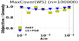
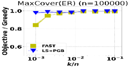
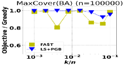
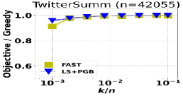
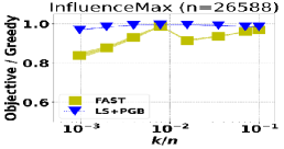
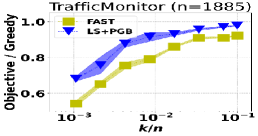
Figure 3: Objective value vs. $k/n$. The objective value is normalized by the standard greedy value. The ($k/n$)-axis is log-scaled.

Fig.4 demonstrates the mean total queries needed by LS+PGB and FAST for all applications with both FAST and LS+PGB exhibiting a linear scaling behavior with the increasing $k$ values with the magnitude of rise in total queries with $k$ is less than 5 folds even with 100 folds increase in $k$. Overall as shown in table 2, LS+PGB achieves the objective in less than half the total queries required by FAST for the MaxCover and the TwitterSumm objective. Whereas for TrafficMonitor and InfluenceMax, FAST requires 1.5 and 1.9 times the queries needed by LS+PGB for the same objective. Very similar in nature to the number of query calls, as shown in fig. 6 - 6, LS+PGB either maintains or outperforms FAST across all the applications.

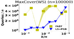
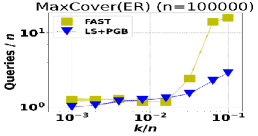
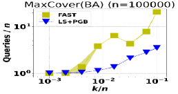
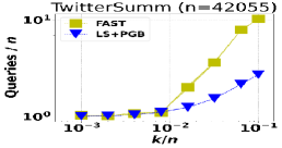
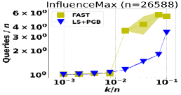
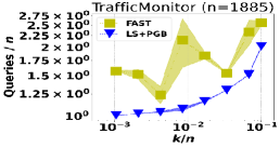
Figure 4: Total Queries/ $n$ vs. $k/n$. Both axes are log-scaled.

Fig. 5 and 6 illustrates the adaptivity and the parallel runtime of LS+PGB and FAST across the six datasets. As shown in fig. 6, both algorithms exhibit linear scaling of runtime with $k$. Overall on an average over the six datasets, FAST requires more than 3 times the time needed by LS+PGB to achieve the objective with TwitterSumm being the objective where overall LS+PGB is over 4 times quicker than FAST. In terms of adaptivity, as demonstarted in fig. 5, especially for larger values $k$, FAST requires more than double the adaptive rounds needed by LS+PGB for the MaxCover and TwitterSumm application. For InfluenceMax and TrafficMonitor, LS+PGB either maintans or outperforms FAST for larger $k$ values.

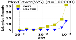
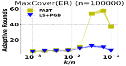
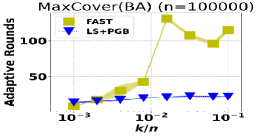
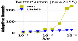
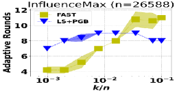
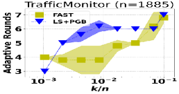
Figure 5: Adaptive Rounds vs. $k/n$. The ($k/n$)-axis is log-scaled.

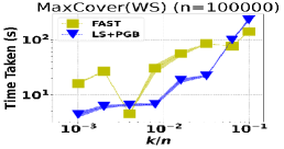
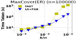
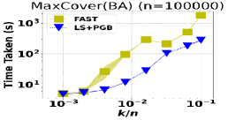
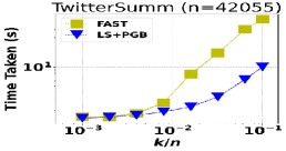
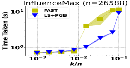
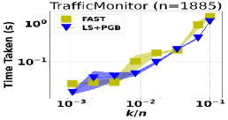
Figure 6: Parallel Runtime vs. $k/n$. Both axes are log-scaled.

H.4 Time vs. Number of Threads

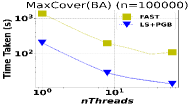
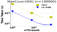
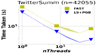
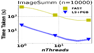
Figure 7: Runtime (s) vs. number of processors. Both axes are log-scaled.

This experiment set aims to demonstrate the improvement in parallel run time taken by the algorithms to solve the application with increasing number of available threads. We use the SM: maximum cover on random graphs (MaxCover), twitter feed summarization (TweetSumm), image summarization (ImageSumm). See Appendix H.2 for the definition of the objectives. All experiments were conducted with a constant $k$ value of 1,000 and the number of available threads provided to the algorithms ranged from 1 to 64 threads, doubling the number of threads for each interval in between. The parallel run time of the experiments is measured in seconds. As shown in fig. 7, the scaling behavior of both FAST and LS+PGB are very similar with the number of processors employed, each algorithm exhibiting a linear speedup initially with the number of processors, which plateaus past a certain number of processors. LS+PGB outperforms FAST across all instances with an average speedup of 10 over FAST.

H.5 Comparison vs adaptive algorithms from Fahrbach et al. [17]

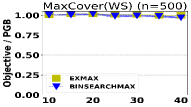
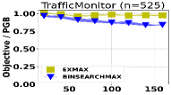
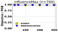
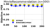
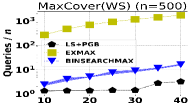
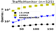
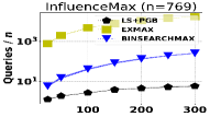
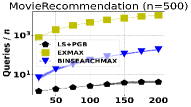
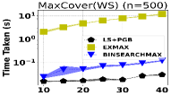
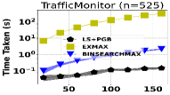
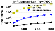
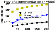
Figure 8: Evaluation of adaptive algorithms from Fahrbach et al. [17] on MaxCover(WS), TrafficMonitor, InfluenceMax and MovieRecommendation in terms of objective value normalized by the standard greedy value (Figure 8 - 8), total number of queries (Figure 8 - 8) and the time required by each algorithm (Figure 8 - 8)

Since ExhaustiveMaximization and the BinarySearchMaximization algorithm of Fahrbach et al. [17] has better theoretical guarantee than FAST, we ran additional experiments comparing against both the ExhaustiveMaximization and the BinarySearchMaximization algorithm, as implemented by the authors of FAST. In this highly optimized implementation, a single query per processor is used in each adaptive round instead of the number of queries required theoretically as description of the implementation in Breuer et al. [9]. The evaluation was performed on MaxCover(WS), TrafficMonitor, InfluenceMax and MovieRecommendation in terms of objective value normalized by the standard greedy value (Figure 8 - 8), total number of queries (Figure 8 - 8) and the time required by each algorithm. In summary, our algorithm LS+PGB is faster by roughly an order of magnitude and uses roughly an order of magnitude fewer queries over BinarySearchMaximization.

References

- [1] CalTrans. Pems: California performance measuring system. http://pems.dot.ca.gov/. [Online; accessed 1-May-2018].
- Badanidiyuru and Vondrák [2014] Ashwinkumar Badanidiyuru and Jan Vondrák. Fast algorithms for maximizing submodular functions. In ACM-SIAM Symposium on Discrete Algorithms (SODA), 2014.
- Balkanski and Singer [2018] Eric Balkanski and Yaron Singer. The adaptive complexity of maximizing a submodular function. In ACM SIGACT Symposium on Theory of Computing (STOC), 2018.
- Balkanski et al. [2018] Eric Balkanski, Adam Breuer, and Yaron Singer. Non-monotone submodular maximization in exponentially fewer iterations. In Advances in Neural Information Processing Systems 31: Annual Conference on Neural Information Processing Systems 2018, NeurIPS 2018, December 3-8, 2018, Montréal, Canada, pages 2359–2370, 2018.
- Balkanski et al. [2019a] Eric Balkanski, Aviad Rubinstein, and Yaron Singer. An Exponential Speedup in Parallel Running Time for Submodular Maximization without Loss in Approximation. In ACM-SIAM Symposium on Discrete Algorithms (SODA), 2019a.
- Balkanski et al. [2019b] Eric Balkanski, Aviad Rubinstein, and Yaron Singer. An optimal approximation for submodular maximization under a matroid constraint in the adaptive complexity model. In Proceedings of the Annual ACM Symposium on Theory of Computing, pages 66–77, nov 2019b.
- Barbosa et al. [2015] Rafael Barbosa, Alina Ene, Huy Le Nguyen, and Justin Ward. The Power of Randomization: Distributed Submodular Maximization on Massive Datasets. In International Conference on Machine Learning (ICML), 2015.
- Barbosa et al. [2016] Rafael Da Ponte Barbosa, Alina Ene, Huy L. Nguyen, and Justin Ward. A New Framework for Distributed Submodular Maximization. In IEEE Symposium on Foundations of Computer Science (FOCS), 2016.
- Breuer et al. [2019] Adam Breuer, Eric Balkanski, and Yaron Singer. The FAST Algorithm for Submodular Maximization. In International Conference on Machine Learning (ICML), 2019.
- Calinescu et al. [2007] Gruia Calinescu, Chandra Chekuri, Martin Pál, and Jan Vondrák. Maximizing a Submodular Set Function subject to a Matroid Constraint. In Integer Programming and Combinatorial Optimization (IPCO), pages 182–196, 2007.
- Chekuri and Quanrud [2019] Chandra Chekuri and Kent Quanrud. Submodular function maximization in parallel via the multilinear relaxation. In Proceedings of the Annual ACM-SIAM Symposium on Discrete Algorithms (SODA), pages 303–322, jul 2019.
- Conforti and Cornuéjols [1984] Michele Conforti and Gérard Cornuéjols. Submodular set functions, matroids and the greedy algorithm: Tight worst-case bounds and some generalizations of the Rado-Edmonds theorem. Discrete Applied Mathematics, 7(3):251–274, 1984.
- Dean and Ghemawat [2008] Jeffrey Dean and Sanjay Ghemawat. MapReduce: Simplified Data Processing on Large Clusters. Communications of the ACM, 51(1):107–113, 2008.
- Ene and Nguyen [2019] Alina Ene and Huy L Nguyen. Submodular Maximization with Nearly-optimal Approximation and Adaptivity in Nearly-linear Time. In ACM-SIAM Symposium on Discrete Algorithms (SODA), 2019.
- Ene and Nguyên [2020] Alina Ene and Huy L. Nguyên. Parallel Algorithm for Non-Monotone DR-Submodular Maximization. In International Conference on Machine Learning (ICML), 2020.
- Epasto et al. [2017] Alessandro Epasto, Vahab Mirrokni, and Morteza Zadimoghaddam. Bicriteria Distributed Submodular Maximization in a Few Rounds. In Symposium on Parallelism in Algorithms and Architectures (SPAA), 2017.
- Fahrbach et al. [2019a] Matthew Fahrbach, Vahab Mirrokni, and Morteza Zadimoghaddam. Submodular Maximization with Nearly Optimal Approximation, Adaptivity, and Query Complexity. In ACM-SIAM Symposium on Discrete Algorithms (SODA), pages 255–273, 2019a.
- Fahrbach et al. [2019b] Matthew Fahrbach, Vahab Mirrokni, and Morteza Zadimoghaddam. Non-monotone Submodular Maximization with Nearly Optimal Adaptivity Complexity. In International Conference on Machine Learning (ICML), 2019b.
- Fahrbach et al. [2019c] Matthew Fahrbach, Vahab Mirrokni, and Morteza Zadimoghaddam. Non-monotone submodular maximization with nearly optimal adaptivity and query complexity. In International Conference on Machine Learning, pages 1833–1842. PMLR, 2019c.
- Gillenwater et al. [2012] Jennifer Gillenwater, Alex Kulesza, and Ben Taskar. Near-Optimal MAP Inference for Determinantal Point Processes. In Advances in Neural Information Processing Systems (NeurIPS), 2012.
- Horel and Singer [2016] Thibaut Horel and Yaron Singer. Maximization of Approximately Submodular Functions. In Advances in Neural Information Processing Systems (NeurIPS), 2016.
- Kazemi et al. [2019] Ehsan Kazemi, Marko Mitrovic, Morteza Zadimoghaddam, Silvio Lattanzi, and Amin Karbasi. Submodular Streaming in All its Glory: Tight Approximation, Minimum Memory and Low Adaptive Complexity. In International Conference on Machine Learning (ICML), 2019.
- Krause and Guestrin [2007] Andreas Krause and Carlos Guestrin. Near-optimal observation selection using submodular functions. AAAI Conference on Artificial Intelligence, 2007.
- Kuhnle [2021a] Alan Kuhnle. Quick Streaming Algorithms for Maximization of Monotone Submodular Functions in Linear Time. In Artificial Intelligence and Statistics (AISTATS), 2021a.
- Kuhnle [2021b] Alan Kuhnle. Nearly Linear-Time, Parallelizable Algorithms for Non-Monotone Submodular Maximization. In AAAI Conference on Artificial Intelligence, 2021b.
- Leskovec et al. [2007] Jure Leskovec, Andreas Krause, Carlos Guestrin, Christos Faloutsos, Jeanne VanBriesen, and Natalie Glance. Cost-effective Outbreak Detection in Networks. In ACM SIGKDD International Conference on Knowledge Discovery and Data Mining (KDD), 2007.
- Minoux [1978] Michel Minoux. Accelerated greedy algorithms for maximizing submodular set functions. In Optimization techniques, pages 234–243. Springer, 1978.
- Mirrokni and Zadimoghaddam [2015] Vahab Mirrokni and Morteza Zadimoghaddam. Randomized Composable Core-Sets for Distributed Submodular Maximization. In ACM Symposium on Theory of Computing (STOC), 2015.
- Mirzasoleiman et al. [2016] Baharan Mirzasoleiman, Ashwinkumar Badanidiyuru, and Amin Karbasi. Fast constrained submodular maximization: Personalized data summarization. In International Conference on Machine Learning, pages 1358–1367. PMLR, 2016.
- Mirzasoleiman et al. [2018] Baharan Mirzasoleiman, Stefanie Jegelka, and Andreas Krause. Streaming Non-Monotone Submodular Maximization: Personalized Video Summarization on the Fly. In AAAI Conference on Artificial Intelligence, 2018.
- Mitzenmacher and Upfal [2017] Michael Mitzenmacher and Eli Upfal. Probability and computing: Randomization and probabilistic techniques in algorithms and data analysis. Cambridge university press, 2017.
- Nemhauser and Wolsey [1978] G L Nemhauser and L A Wolsey. Best Algorithms for Approximating the Maximum of a Submodular Set Function. Mathematics of Operations Research, 3(3):177–188, 1978.
- Rossi and Ahmed [2015] Ryan Rossi and Nesreen Ahmed. The network data repository with interactive graph analytics and visualization. In Proceedings of the AAAI Conference on Artificial Intelligence, volume 29, 2015.
- Wald [1945] Abraham Wald. Some generalizations of the theory of cumulative sums of random variables. The Annals of Mathematical Statistics, 16(3):287–293, 1945.