The static force from generalized Wilson loops

Abstract

Recently a method to compute the static force with lattice gauge theory using an insertion of a chromoelectric field into a Wilson loop was proposed. We explore this method using the multilevel algorithm and discuss the renormalization of the chromoelectric field on the lattice.

1 Introduction

The potential between a static quark-antiquark pair $V(r)$ is one of the most commonly studied quantities in QCD. At small separations $r$ the static potential can be calculated in a weak coupling expansion. The perturbative expression of the static energy is known at N³LL accuracy and can be combined with high precision measurements of the same quantity in lattice QCD. This allows an accurate extraction of the strong coupling $\alpha_{\rm s}$, which is competitive with lattice determinations from different observables [1].

In a lattice regularization, the static potential comes with a linear divergence of order $\alpha_{\rm s}(1/a)/a$ (with $a$ denoting the lattice spacing) also referred to as self-energy. The self-energy vanishes in dimensional regularization. However, the perturbative expression for $V(r)$ in dimensional regularization is affected by a renormalon ambiguity of order $\Lambda_{\text{QCD}}$ [2, 3]. Both the renormalon and the self energy can be absorbed into an additive constant. This constant disappears, when considering the static force $F(r)=\partial_{r}V(r)$. The static force encodes the shape of $V(r)$ and carries all the physical information needed to extract $\alpha_{\text{s}}$, while being finite and renormalon free.

A precise computation of the static force on the lattice can be challenging. While the traditional way of computing the static force by taking finite differences of the static potential [4, 5] can be efficient in quenched lattice QCD, the lattice data points for $V(r)$ might be too sparse in full QCD for a reliable extraction of the static force either via finite differences or via interpolation [6]. Such problems can be avoided by using a recently suggested method [7, 8] based on Ref. [9]: The force between a static quark and a static antiquark is computed directly from the expectation value of a Wilson loop with a chromoelectric field inserted in one of the temporal Wilson lines.

In this paper we carry out a quenched lattice QCD computation of the static force using this new method. We discuss, how to obtain the static force either from Wilson or Polyakov loops with chromoelectric field insertions. Both approaches yield consistent results. The corresponding systematic errors are, however, different. We also address the issue that the discretized chromoelectric field has a slow convergence towards the continuum limit, unless a multiplicative renormalization factor is introduced.

This conference contribution is organized in the following way: We introduce our observables in section 2 and the simulation setup in section 3. The renormalization of this definition of the static force is discussed in section 4. Numerical results for the static force are presented in section 5. Further details can be found in our recent publication [10]. Results obtained at an early stage of this project were discussed at a previous edition of the lattice conference [11].

2 Observables and their discretizations

The force $F(r)$ between a static quark and an antiquark is the derivative of the static potential $V(r)$,

$$F(r)=\partial_{r}V(r).$$ (1)

$V(r)$ is related to rectangular Wilson loops with large temporal extent $T$ and arbitrary spatial extent $r$,

$$e^{-V(r)T}\sim{\rm Tr}\{{\rm P}\,W_{r\times T}\}={\rm Tr}\bigg{\{}{\rm P}\,\exp\bigg{(}ig\oint_{r\times T}dx_{\mu}\,A_{\mu}(x)\bigg{)}\bigg{\}}.$$ (2)

On a lattice the Wilson loop $W_{r\times T}$ is discretized by a product of link variables $U_{\mu}(x)=e^{iagA_{\mu}(x)}$. The static potential is typically extracted via

$$V(r,a)=\lim_{T\rightarrow\infty}V_{\text{eff}}(r,T,a)\quad,\quad V_{\text{eff}}(r,T,a)=-\frac{1}{a}\ln\frac{\langle\textrm{Tr}\{{\rm P}\,W_{r\times(T+a)}\}\rangle}{\langle\textrm{Tr}\{{\rm P}\,W_{r\times T}\}\rangle}.$$ (3)

The static force can the be obtained in a straightforward way from the static potential by using a discrete derivative, e.g.

$$F_{\partial V}(r,a)=\frac{V(r+a,a)-V(r-a,a)}{2a}.$$ (4)

Alternatively, one can compute the static force using a method proposed in Refs. [7, 8],

$$F(r)=\lim_{T\rightarrow\infty}-i\frac{\langle{\rm Tr}\{{\rm P}\,W_{r\times T}\,\hat{\mathbf{r}}\cdot g\mathbf{E}(\mathbf{r},t^{\ast})\}\rangle}{\langle\textrm{Tr}\{{\rm P}\,W_{r\times T}\}\rangle}\,.$$ (5)

Here $\hat{\mathbf{r}}$ is the spatial direction of the separation of the static quark-antiquark pair and $\mathbf{E}(\mathbf{r},t^{\ast})$ denotes the chromoelectric field inserted on one of the temporal Wilson lines at a fixed time $t^{\ast}$. The chromoelectric field components are defined as $E_{j}(x)=F_{j0}(x)$ in terms of the non-Abelian field strength tensor. We note that $\langle{\rm Tr}\{{\rm P}\,W_{r\times T}\,gE_{j}({\bf r},t^{*})\}\rangle$ depends on $t^{\ast}$. This dependence, however, disappears in the limit $T\rightarrow\infty$, if $t^{\ast}$ is kept constant.

The lattice formulation of the right hand side of Eq. (5) requires a discretized field insertion $E_{j}$. We use two different symmetric formulations, a so-called butterfly

$$\Pi_{j0}=\frac{P_{j,0}+P_{0,-j}}{2}$$ (6)

or a cloverleaf

$$\Pi_{j0}=\frac{P_{j,0}+P_{0,-j}+P_{-j,-0}+P_{-0,j}}{4}$$ (7)

of plaquettes $P_{\mu,\nu}=1+ia^{2}gF_{\mu\nu}+\mathcal{O}(a^{4})=U_{\mu}(x)U_{\nu}(x+\hat{\mu})U^{\dagger}_{\mu}(x+\hat{\nu})U_{\nu}^{\dagger}(x)$ [12]. In both cases the chromoelectric field is given by

$$gE_{j}=\frac{\Pi_{j0}-\Pi^{\dagger}_{j0}}{2ia^{2}}+\mathcal{O}(a^{2}).$$ (8)

Moreover, it is convenient to define an effective force and to extract the static force via

$$F_{E}(r,a)=\lim_{T\rightarrow\infty}F_{E,\text{eff}}(r,T,a)\quad,\quad F_{E,\text{eff}}(r,T,a)=-i\frac{\langle\textrm{Tr}\{{\rm P}\,W_{r\times T}\,\hat{\mathbf{r}}\cdot g\mathbf{E}(\mathbf{r},t^{*})\}\rangle}{\langle\textrm{Tr}\{{\rm P}\,W_{r\times T}\}\rangle}.$$ (9)

In the following we insert the chromoelectric field $\mathbf{E}(\mathbf{r},t^{*})$ exclusively at $t^{*}=0$. While the continuum formulation (5) is independent of $t^{*}$, the choice $t^{*}=0$ maximizes the the distance to both temporal boundaries of the Wilson loop and, thus, should lead to a stronger suppression of excitations and, consequently, to a clearer signal. Furthermore, we improve the lattice results for the static force using perturbation theory at tree-level. This is done by redefining the discrete lattice separations $r$ in such a way that the right-hand-side of Eq. (5) in lattice tree-level perturbation theory and in continuum tree-level perturbation theory are identical.

Instead of Wilson loops one can also consider correlation functions of Polyakov loops to compute the static potential as well as the static force. A Polyakov loop is defined as the normalized trace of a closed temporal Wilson line winding around the periodic temporal direction of extent $T$,

$$L({\bf x})=\frac{1}{N_{c}}{\rm Tr}\bigg{\{}{\rm P}\,\exp\bigg{(}ig\int_{0}^{T}dt\,A_{0}(x)\bigg{)}\bigg{\}}.$$ (10)

For the static force a Polyakov loop with a chromoelectric field insertion is needed,

$$L_{E}(\mathbf{r})=\frac{1}{N_{c}}{\rm Tr}\bigg{\{}{\rm P}\,\exp\bigg{(}ig\int_{t^{*}}^{T}dt\,A_{0}(x)\bigg{)}\hat{\mathbf{r}}\cdot g\mathbf{E}(\mathbf{r},t^{*}){\rm P}\,\exp\bigg{(}ig\int_{0}^{t^{*}}dt\,A_{0}(x)\bigg{)}\bigg{\}}.$$ (11)

The analogue of Eq. (5) then reads

$$F(r)=\lim_{T\rightarrow\infty}-i\frac{\langle L^{\dagger}({\bf 0})L_{E}(\mathbf{r})\rangle}{\langle L^{\dagger}({\bf 0})L(\mathbf{r})\rangle}.$$ (12)

3 Simulation setup

We discretize the SU(3) Yang-Mills theory using the standard Wilson plaquette action. We carried out simulations with the multilevel algorithm [13], where we performed the updates using the heatbath and overrelaxation algorithms. We generated three ensembles with lattice spacings $a=0.060\,\text{fm}$, $a=0.048\,\text{fm}$ and $a=0.040\,\text{fm}$, which we refer to as ensembles $A$, $B$, and $C$, respectively. The lattice spacing in units of the scale $r_{0}$ is related to the gauge coupling $\beta$ with a parameterization from Ref. [4]. The full set of simulation parameters for the ensembles $A$, $B$, and $C$ can be found in Ref. [10].

To improve the ground state overlaps generated by the spatial Wilson lines in the Wilson loops, we use APE smeared spatial links with $\alpha_{\textrm{APE}}=0.5$ and $N_{\textrm{APE}}=50$ smearing steps for the Wilson loops (for detailed equations see e.g. Ref. [14]).

4 Renormalization

On the lattice the two definitions of the static force, $F_{E}(r,a)$ and $F_{\partial V}(r,a)$ ((9) and (4), respectively), lead to significantly different discretization errors. In other words, the convergence of these observables to the continuum result is quite different. Such differences are expected, because it is known that observables involving components of the field strength tensor often exhibit sizable discretization errors at values of the gauge coupling typically used in numerical simulations. The reason is the slow convergence of lattice perturbation theory, when expanded in the bare coupling [15]. To reduce discretization errors arising from chromoelectric and chromomagnetic field insertions, one can use multiplicative renormalization or improvement factors as discussed in Refs. [16, 12, 17, 18, 19].

We define such a multiplicative improvement factor $Z_{\textrm{E}}$ corresponding to a finite renormalization via

$$Z_{\textrm{E}}(a)=\frac{F_{\partial V}(r^{\ast},a)}{F_{E}(r^{\ast},a)},$$ (13)

where $r^{\ast}$ is an arbitrary separation. After determining this renormalization factor $Z_{\textrm{E}}(a)$ at a single arbitrary separation $r^{\ast}$, it can be used to improve $F_{E}(r,a)$ at all other separations according to

$$F_{E}^{\text{ren}}(r,a)=Z_{\textrm{E}}(a)F_{E}(r,a).$$ (14)

$F_{E}^{\text{ren}}(r,a)$ should then have significantly smaller discretization errors than $F_{E}(r,a)$ and, thus, is expected to be quite close to both $F_{\partial V}(r,a)$ and the continuum result $F(r)$. We note that $Z_{\textrm{E}}(a)\rightarrow 1$ for $a\rightarrow 0$.

In Fig. 1 we show the renormalization constant $Z_{\textrm{E}}$, defined in Eq. (13), as a function of $r^{\ast}$ for both Wilson and Polyakov loops. The figure exhibits plateau regions that confirm the expected constant behavior of $Z_{\textrm{E}}$. Also consistent with expectation is the dependence of $Z_{\textrm{E}}$ on $\beta$. One can see that with decreasing lattice spacing $a$ the improvement factor $Z_{\textrm{E}}$ slowly decreases towards $1$.

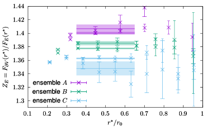
Figure 1: $Z_{\textrm{E}}=F_{\partial V}/F_{E}$ as a function of $r^{\ast}$. The colored horizontal lines and error bands represent the fits to determine a numerical value for $Z_{\textrm{E}}$ for each ensemble. (left) Wilson loops. (right) Polyakov loops.

We determine a numerical value for $Z_{\textrm{E}}$ for each ensemble by fitting a constant to the lattice data points shown in Fig. 1 in the range $0.35\,r_{0}\leq r^{\ast}\leq 0.65\,r_{0}$. Results of these fits are collected in Table 1 for both Wilson and Polyakov loops. There are small differences between the Wilson loop and the Polyakov loop results, which might be due to different remaining systematic errors.

ensemble	$a$ in fm	$Z_{\textrm{E}}$ from Wilson loops	$Z_{\textrm{E}}$ from Polyakov loops
A	$0.060$	$1.4068(63)$	$1.4001(20)$
B	$0.048$	$1.3853(30)$	$1.3776(10)$
C	$0.040$	$1.348(11)\phantom{0}$	$1.3628(13)$

Table 1: Renormalization constants $Z_{\textrm{E}}$ obtained by fitting constants to $F_{\partial V}/F_{E}$ in the range $0.35\,r_{0}\leq r^{\ast}\leq 0.65\,r_{0}$.

5 Numerical results for the static force

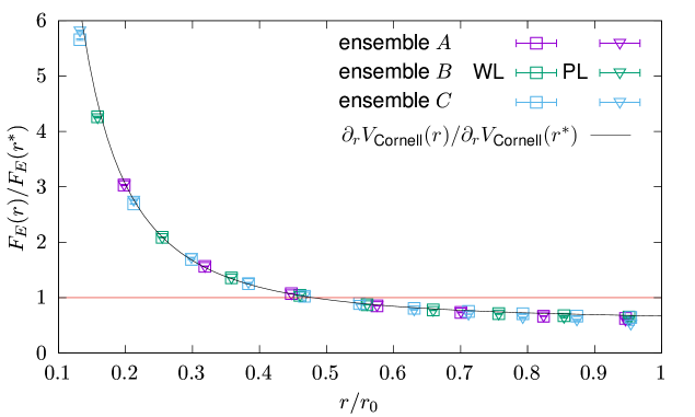
Figure 2: Left: $F_{E}(r)/F_{E}(r^{\ast})$ as a function of $r$ for $r^{\ast}=0.48\,r_{0}\approx 0.24\,\textrm{fm}$ obtained from Wilson loops (boxes) and Polyakov loops (triangles). For comparison we also show $\partial_{r}V_{\textrm{Cornell}}(r)/\partial_{r}V_{\textrm{Cornell}}(r^{\ast})$.

Now we consider $F_{E}(r)/F_{E}(r^{\ast})$, where $F_{E}$ is the non-renormalized static force defined in Eq. (9). We choose a fixed separation $r^{\ast}=0.48\,r_{0}\approx 0.24\,\textrm{fm}$ such that $r^{\ast}/a$ is close to an integer for all three ensembles. Corresponding numerical results for Wilson loops as well as for Polyakov loops are shown in Fig. 2. For comparison, we also fit a Cornell ansatz $V_{\textrm{Cornell}}(r)=-\alpha/r+\sigma r$ to the static potential and plot $\partial_{r}V_{\textrm{Cornell}}(r)/\partial_{r}V_{\textrm{Cornell}}(r^{\ast})$. The agreement of $F_{E}(r)/F_{E}(r^{\ast})$ and $\partial_{r}V_{\textrm{Cornell}}(r)/\partial_{r}V_{\textrm{Cornell}}(r^{\ast})$ constitutes a numerical proof of concept for the method of computing the static force via a chromoelectric field insertion.

In summary, we tested a novel method to compute the static force $F(r)$ from expectation values of Wilson or Polyakov loops with chromoelectric field insertions. The numerical results exhibit sizable discretization errors and the convergence to the continuum limit is rather slow, but this can be compensated by an $r$-independent multiplicative renormalization factor $Z_{\textrm{E}}$. Concerning efficiency, our method appears to be comparable to the traditional method of first computing the static potential and then taking the derivative, as investigated and discussed in detail in our recent publication [10]. We note that the relation between the force and the color electric field has also been used in recent work from other groups [20, 21] to determine the string tension.

This exploratory computation of the static force is also an important preparatory step for future projects, where similar correlation functions need to be computed. An example is the computation of $1/m$ and $1/m^{2}$ corrections ($m$ denotes the heavy quark mass) to the ordinary static potential or to hybrid static potentials. We conclude by noting that the renormalization discussed in section 4 might not be necessary anymore, when using the gradient flow, as discussed during the conference talk. Due to page limitations we do not discuss the gradient flow in the context of the static force in this proceedings contribution, but refer to the forthcoming Ref. [22].

References

- [1] Flavour Lattice Averaging Group collaboration, S. Aoki et al., FLAG Review 2019, 1902.08191.
- [2] A. Pineda, Heavy quarkonium and nonrelativistic effective field theories, phd thesis, University of Barcelona, 1998.
- [3] A. H. Hoang, M. C. Smith, T. Stelzer and S. Willenbrock, Quarkonia and the pole mass, Phys. Rev. D 59 (1999) 114014 [hep-ph/9804227].
- [4] S. Necco and R. Sommer, The heavy quark potential from short to intermediate distances, Nucl. Phys. B622 (2002) 328 [hep-lat/0108008].
- [5] S. Necco and R. Sommer, Testing perturbation theory on the static quark potential, Phys. Lett. B 523 (2001) 135 [hep-ph/0109093].
- [6] A. Bazavov, N. Brambilla, X. G. Tormo, I, P. Petreczky, J. Soto and A. Vairo, Determination of from the QCD static energy: An update, Phys. Rev. D 90 (2014) 074038 [1407.8437].
- [7] A. Vairo, A low-energy determination of at three loops, EPJ Web Conf. 126 (2016) 02031 [1512.07571].
- [8] A. Vairo, Strong coupling from the QCD static energy, Mod. Phys. Lett. A31 (2016) 1630039.
- [9] N. Brambilla, A. Pineda, J. Soto and A. Vairo, The QCD potential at O(1/m), Phys. Rev. D63 (2001) 014023 [hep-ph/0002250].
- [10] N. Brambilla, V. Leino, O. Philipsen, C. Reisinger, A. Vairo and M. Wagner, Lattice gauge theory computation of the static force, 2106.01794.
- [11] TUMQCD collaboration, N. Brambilla, V. Leino, O. Philipsen, C. Reisinger, A. Vairo and M. Wagner, Static force from the lattice, PoS LATTICE2019 (2019) 109 [1911.03290].
- [12] G. S. Bali, K. Schilling and A. Wachter, Complete corrections to the static interquark potential from SU(3) gauge theory, Phys. Rev. D56 (1997) 2566 [hep-lat/9703019].
- [13] M. Lüscher and P. Weisz, Locality and exponential error reduction in numerical lattice gauge theory, JHEP 09 (2001) 010 [hep-lat/0108014].
- [14] ETM collaboration, K. Jansen, C. Michael, A. Shindler and M. Wagner, The Static-light meson spectrum from twisted mass lattice QCD, JHEP 12 (2008) 058 [0810.1843].
- [15] G. P. Lepage and P. B. Mackenzie, On the viability of lattice perturbation theory, Phys. Rev. D 48 (1993) 2250 [hep-lat/9209022].
- [16] A. Huntley and C. Michael, Spin - Spin and Spin - Orbit Potentials From Lattice Gauge Theory, Nucl. Phys. B286 (1987) 211.
- [17] Y. Koma and M. Koma, Spin-dependent potentials from lattice QCD, Nucl. Phys. B769 (2007) 79 [hep-lat/0609078].
- [18] ALPHA collaboration, D. Guazzini, H. B. Meyer and R. Sommer, Non-perturbative renormalization of the chromo-magnetic operator in Heavy Quark Effective Theory and the B* - B mass splitting, JHEP 10 (2007) 081 [0705.1809].
- [19] C. Christensen and M. Laine, Perturbative renormalization of the electric field correlator, Phys. Lett. B 755 (2016) 316 [1601.01573].
- [20] M. Baker, P. Cea, V. Chelnokov, L. Cosmai, F. Cuteri and A. Papa, Isolating the confining color field in the SU(3) flux tube, Eur. Phys. J. C 79 (2019) 478 [1810.07133].
- [21] M. Baker, P. Cea, V. Chelnokov, L. Cosmai, F. Cuteri and A. Papa, The confining color field in SU(3) gauge theory, Eur. Phys. J. C 80 (2020) 514 [1912.04739].
- [22] V. Leino, N. Brambilla, J. Mayer-Steudte and A. Vairo, The static force from generalized Wilson loops using gradient flow, In preparation TUM-EFT 157/21 (2021) .