Pseudo-peakons and Cauchy analysis for an integrable fifth-order equation of Camassa-Holm type

Abstract

In this paper, we discuss integrable higher order equations of Camassa-Holm (CH) type. Our higher order CH-type equations are “geometrically integrable”, that is, they describe one-parametric families of pseudo-spherical surfaces, in a sense explained in Section 1, and they are integrable in the sense of zero curvature formulation ($\simeq$ Lax pair) with infinitely many local conservation laws. The major focus of the present paper is on a specific fifth order CH-type equation admitting pseudo-peakons solutions, that is, weak bounded solutions with differentiable first derivative and continuous and bounded second derivative, but such that any higher order derivative blows up. Furthermore, we investigate the Cauchy problem of this fifth order CH-type equation on the real line and prove local well-posedness under the initial conditions $u_{0}\in H^{s}({\mathbb{R}})$, $s>7/2$. In addition, we study conditions for global well-posedness in $H^{4}({\mathbb{R}})$ as well as conditions causing local solutions to blow up in a finite time. We conclude our paper with some comments on the geometric content of the high order CH-type equations.

Keywords: Camassa-Holm equation; equations of pseudo-spherical type; local conservation laws; pseudo-peakons; fifth order CH-type equation; well-posedness.

AMS Classification: 35G25, 35L05, 35Q53.

1 Introduction

In this paper we present a family of fifth-order integrable equations which generalize —in a very precise sense discussed below— the celebrated Camassa-Holm (CH) equation (see [5])

$$\tilde{m}_{t}=-\tilde{m}_{x}\,u-2\,\tilde{m}\,u_{x}\;,\quad\quad\tilde{m}=u_{xx}-u\;.$$ (1)

Here and at the beginning of Section 2 we use $\tilde{m}$ instead of $m$ when considering the CH equation in order to keep the signs used in [27], and not to cause confusion with the conventions used in the main body of this paper.

Our original motivation for undertaking this project was the observation that the Camassa-Holm equation can be understood as an Euler equation for the inertia operator $A_{2}=\partial_{xx}-1$ on the Lie algebra $Vect(S^{1})$ of the (Fréchet) Lie group $Diff(S^{1})$, and that, in turn, the latter equation can be interpreted geometrically as determining geodesics for a Riemannian metric on $Diff(S^{1})$ defined via $A_{2}\,$, see for instance [1, 20, 23], and also [16]. Now, the operator $A_{2}$ appears naturally in the zero curvature representation of CH, see Equations (14) and (15) below. A rather obvious question that arises is whether considering different inertia operators $A_{n}$ in (14) and (15) would yield equations that may be of interest for the theory of fluids and may determine interesting geometry on diffeomorphism groups.

We can think of two immediate objections to considering this question. First: Wouldn’t changing just the inertia operator used in (14) and (15) yield equations “equivalent” to CH? Second: Wouldn’t we obtain only uninteresting equations, since in the paper [13] Constantin and Kolev proved that in the case of $Vect(S^{1})$ and the (Fréchet) Lie group $Diff(S^{1})$ the only bi-Hamiltonian equations (for some natural Poisson structures) arising from inertia operators $A_{n}=\sum(-1)^{k}\partial_{x}^{2k}$ are the inviscid Burgers equation ($k=0$) and the Camassa-Holm equation ($k=1$)?

The way we have found of replying to these objections is through geometric considerations. It was proven in [27] that the Camassa-Holm (1) describes pseudo-spherical surfaces, in the following sense:

Define three one-forms $\omega^{i}$, $i=1,2,3$, as follows:

$$\omega^{1} = \left(\frac{1}{2}\lambda+\frac{1}{2\lambda}+\tilde{m}\right)dx+\left(-\frac{1}{2\lambda}u+\frac{u}{2}\lambda-u\tilde{m}-\frac{1}{2}-\frac{\lambda^{2}}{2}\right)dt$$ (2)

$$\omega^{2} = -u_{x}dt$$ (3)

$$\omega^{3} = \left(-\frac{1}{2}\lambda+\frac{1}{2\lambda}-\tilde{m}\right)dx+\left(-\frac{1}{2\lambda}u-\frac{u}{2}\lambda+u\tilde{m}-\frac{1}{2}+\frac{\lambda^{2}}{2}\right)dt\;.$$ (4)

Then, the structure equations of a pseudo-spherical surface,

$$d\omega^{1}=\omega^{3}\wedge\omega^{2}\;,\quad\quad d\omega^{2}=\omega^{1}\wedge\omega^{3}\;,\quad\quad d\omega^{3}=\omega^{1}\wedge\omega^{2}\;,$$ (5)

are satisfied if and only if $u(x,t)$ and $\tilde{m}(x,t)$ satisfy the Camassa-Holm equation. The existence of this geometric structure is quite useful for applications: it allows us to obtain quadratic pseudo-potentials, a zero curvature formulation for CH, a sequence of non-trivial local conservation laws, non-local symmetries, and a geometrically motivated modified Camassa-Holm equation, see [27, 18, 17]; see also [30, 15, 24] for independent articles showing zero curvature representations of CH as well.

Now, we can modify the one-forms (2)-(4) in such a way that the structure equations (5) are still equivalent to a scalar equation, by keeping the $\lambda$ dependence unchanged and modifying the coefficients of the Laurent polynomials in $\lambda$ appearing in (2)-(4). We would then say that the new scalar equation generalizes CH. Certainly there are restrictions in order for this plan to make sense: there is no point in changing $u$ for a differentiable function of $u$, for example, since in this case we would get an equation obviously equivalent to CH. But, if we consider modifications of $(\ref{o1})$-$(\ref{o3})$ depending on higher order jets of $u$, we would obtain —in principle— new equations, not related to CH by invertible local transformations.

But perhaps we can change $u$ in completely arbitrary ways, and therefore our idea is just too general and naive to be of interest? No. Hereafter, we restrict ourselves to fifth order equations; the following geometric theorem, to be proven in a separate paper, states precisely how we can modify the coefficients of the Laurent polynomials in $\lambda$ appearing in (2)-(4) in order for the structure equations (5) to be equivalent to a scalar differential equation.

Theorem 1.

The most general fifth order equation of pseudo-spherical type that is equivalent to the structure equations $(\ref{o4})$ with associated one-forms

$$\omega^{1} = \left(a\lambda+\frac{d}{\lambda}+F_{11}\right)dx+\left(\frac{1}{\lambda}G_{11}+G_{12}+\lambda G_{13}+\lambda^{2}G_{14}\right)dt$$

$$\omega^{2} = H(u,u_{x},u_{xx},u_{xxx})dt$$

$$\omega^{3} = \left(-a\lambda+\frac{d}{\lambda}+F_{31}\right)dx+\left(\frac{1}{\lambda}G_{31}+G_{32}+\lambda G_{33}+\lambda^{2}G_{34}\right)dt\;,$$

in which the functions $F_{ij}$ and $G_{ij}$ depend on $u,u_{x},u_{xx},u_{xxx},u_{xxxx}$, is

$$4adD_{t}G_{13}-D_{t}D_{x}^{2}G_{13} = \frac{2}{a}(D_{x}G_{13})(D_{x}^{2}G_{13})+\frac{1}{a}(G_{13}+G_{131})D_{x}^{3}G_{13}$$

$$-12dG_{13}D_{x}G_{13}-8dG_{131}D_{x}G_{13}\;,$$

where $G_{13}$ is an arbitrary function of $u,u_{x},u_{xx}$ satisfying $G_{13,u_{xx}}\neq 0$, $D_{x}$ indicates total derivative with respect to $x$, $G_{131}$ is a constant number, and $a\not=0,d$ are two arbitrary real constants.

The one-forms $\omega^{i}=f_{i1}dx+f_{i2}dt$ associated to Equation $(\ref{se4})$ are determined by

$$f_{11} = {a}{\lambda}+\frac{d}{\lambda}+\frac{1}{2dG_{34}}\left[D_{x}^{2}G_{13}-4adG_{13}-2adG_{131}\right]$$

$$f_{12} = -\frac{d}{a\lambda}(G_{13}+G_{131})-\frac{1}{2adG_{34}}(G_{13}+G_{131})D_{x}^{2}G_{13}+\frac{1}{G_{34}}(G_{13}+G_{131})(2G_{13}+G_{131})$$

$$~{}-\frac{dG_{34}}{a}+G_{13}\lambda-G_{34}\lambda^{2}$$

$$f_{21} = 0$$

$$f_{22} = -\frac{1}{a}D_{x}G_{13}$$

$$f_{31} = -{a}{\lambda}+\frac{d}{\lambda}-\frac{1}{2dG_{34}}\left[D_{x}^{2}G_{13}-4adG_{13}-2adG_{131}\right]$$

$$f_{32} = -\frac{d}{a\lambda}(G_{13}+G_{131})+\frac{1}{2adG_{34}}(G_{13}+G_{131})D_{x}^{2}G_{13}-\frac{1}{G_{34}}(G_{13}+G_{131})(2G_{13}+G_{131})$$

$$~{}-\frac{dG_{34}}{a}-G_{13}\lambda+G_{34}\lambda^{2}$$

where $G_{34}$ is, if fact, a non-zero constant number.

We say that the large non-trivial family of fifth order equations of geometric origin (1) are “higher order CH-type equations”, or, that they are “fifth order manifestations” of CH.

Let us now answer the objections raised at the beginning of this section. Equations (1) are not equivalent to CH, as they are only related to CH by non-invertible differential substitutions: if we set $v=G_{13}(u,u_{x},u_{xx})$ in (1), we find that $v$ satisfies (up to some parameters) the CH equation, but there is no reason to expect that the “internal” properties of (1) and CH are the same. Also, the existence of the one-forms $\omega^{i}$ satisfying (5) allow us to check using [9] that Equations (1) admit zero curvature representations. The existence of these zero curvature representations imply the integrability of our corresponding “higher order CH-type equations”, not in the sense of being bi-Hamiltonian, but in the sense of possessing an infinite number of non-trivial local conservation laws. We do lose the interpretation of our higher order CH-type equations as standard Euler equations but, as we show in the last section of this work, the equations considered here can also be connected with the geometry of $Diff(S^{1})$.

In this paper we consider the following fifth order equation of CH-type arising from $(\ref{se4})\,$:

$$\left\{\begin{array}[]{l}m_{t}=-m_{x}v-2mv_{x},\\ v=u-u_{xx}=(1-\partial^{2})u=-A_{2}(u),\\ m=v-v_{xx}=(1-\partial^{2})^{2}u=A_{4}(u)\;.\end{array}\right.$$ (10)

The expansion of (10) reads

$$u_{t}-2u_{{xxt}}+u_{xxxxt} = -3uu_{x}+4uu_{xxx}-uu_{xxxxx}+5u_{x}u_{xx}-2u_{x}u_{xxxx}$$ (11)

$$-6u_{xx}u_{{xxx}}+2u_{xxx}u_{xxxx}+u_{xx}u_{xxxxx}\;.$$

This equation is obtained from (1) if we choose $G_{13}=u-u_{xx}$, $a=1$, $d=1/4$ and $G_{131}=0$. We decided to make this choice partially motivated by [22, 33] where the authors study the model

$$m_{t}+um_{x}+bu_{x}m=0\;,\quad\quad m=(1-\alpha^{2}\partial_{x}^{2})(1-\beta^{2}\partial_{x}^{2})u\;.$$ (12)

We consider Equation (10) in Section 2, where we show that it admits a Lax pair, as anticipated in this section, and that it possesses an infinite number of non-trivial local conservation laws; we also present its Lie algebra of classical symmetries and comment on (the no existence of) nonlocal symmetries of a specific type. Then, in Section $3$ we show that Equation $(\ref{FOCHInt1})$ possesses pseudo-peakons, this is, bounded weak travelling wave solutions with continuous first derivative and continuous second derivative, but whose higher order derivatives blow up. We claim that the existence of this kind of weak solutions, even more than the integrability characteristics of (10), is what makes our equations (1) —and the particular case (11)— of interest. Pseudo-peakons seem to be fairly new objects in the nonlinear landscape; they have been observed before only in the “fifth order Camassa-Holm equation” (12) studied in [22, 33]. It is quite intriguing to find them at the level of Equation (1). In Section 4 we discuss local well-posedness of (10) for initial conditions $u_{0}\in H^{s}({\mathbb{R}})$, $s>7/2$, which is to be contrasted with the corresponding result for standard CH equation: for instance, in [29, Theorem 3.1] local well-posedness of the Camassa-Holm equation is proven for initial data in $H^{s}({\mathbb{R}})$, $s>3/2$. Thus, the “good” spaces of initial data for CH and (10) are different. In this section we also prove a theorem on global well-posedness of (10) in $H^{4}({\mathbb{R}})$, and we present conditions causing local solutions to blow up in a finite time. Finally, in Section 5 we collect several general remarks. We introduce a hierarchy of higher order Camassa-Holm type equations to which (10) belongs, we observe that (in the periodic case, $x\in S^{1}$) these equations are indeed constructed via inertia operators, that our equations can be written in terms of the geometry of the loop group $Diff(S^{1})$, and finally we go back to their relation with classical theory of surfaces.

2 Equations of Camassa–Holm type

Let us begin by recalling the following observation about the important Camassa–Holm equation introduced in [5].

Theorem 2.

The compatibility condition of the linear problem

$$d\psi=(Xdx+Tdt)\psi\;,$$

where $\psi=(\psi_{1},\psi_{2})^{t}$,

$$X=\frac{1}{2}\left[\begin{array}[]{cc}0&\lambda+2\,\tilde{m}\\ \lambda^{-1}&0\end{array}\right]\;,$$ (14)

and

$$T=\frac{1}{2}\left[\begin{array}[]{cc}\displaystyle-{u_{x}}&-2u\,\tilde{m}+\lambda u-\lambda^{2}\\ -1-u\lambda^{-1}&u_{x}\end{array}\right],$$ (15)

is the Camassa-Holm $(CH)$ equation

$$\tilde{m}_{t}=-\tilde{m}_{x}\,u-2\,\tilde{m}\,u_{x}\;,\quad\quad\tilde{m}=u_{xx}-u\;.$$ (16)

This theorem appears in [30] and [27]. As indicated in Section 1, we are using $\tilde{m}$ instead of $m$ here in order to keep the signs used in [27] when discussing CH.

It is well-known how to obtain quadratic pseudo-potentials and conservation laws from associated $sl(2,\mathbb{R})$-valued linear problems, see [9] and Refs. [26, 27] for full details. We obtain:

Theorem 3.

The CH equation $(\ref{reyes:ch})$ admits a quadratic pseudo-potential $\gamma$ determined by the compatible equations

$$\tilde{m}=\gamma_{x}+\frac{1}{2\lambda}\,\gamma^{2}-\frac{1}{2}\lambda\;,\qquad\gamma_{t}=\frac{\gamma^{2}}{2}\left[1+\frac{1}{\lambda}u\right]-u_{x}\gamma-u\,\tilde{m}+\left[\frac{1}{2}u\lambda-\frac{1}{2}\lambda^{2}\right]\,,$$ (17)

where $\lambda\neq 0$ is a parameter. Moreover, Equation $(\ref{reyes:ch})$ possesses the parameter-dependent conservation law

$$\gamma_{t}=\lambda\left(u_{x}-\gamma-\frac{1}{\lambda}u\gamma\right)_{x}.$$ (18)

We can interpret Equations (17) and (18) as determining a “Miura-like” transformation and a “modified Camassa-Holm” (MOCH) model. These observations are developed in [17].

We use (17) and (18) to construct conservation laws for the CH equation. Setting $\gamma=\sum\limits_{n=1}^{\infty}\gamma_{n}\lambda^{n/2}$ and substituting this expansion into (17), we find the conserved densities

$$\gamma_{1}=\sqrt{2}\,\sqrt{\tilde{m}}\;,\qquad\gamma_{2}=-\frac{1}{2}\,\ln(\tilde{m})_{x}\;,\qquad\gamma_{3}=\frac{1}{2\sqrt{2}\,\sqrt{\tilde{m}}}\left[1-\frac{\tilde{m}_{x}^{2}}{4\,\tilde{m}^{2}}+\ln(\tilde{m})_{xx}\right],$$ (19)

$$\gamma_{n+1}=-\frac{1}{\gamma_{1}}\,\gamma_{n,x}-\frac{1}{2\gamma_{1}}\sum_{j=2}^{n}\gamma_{j}\,\gamma_{n+2-j}\;,\qquad n\geq 3\;,$$ (20)

while the expansion $\gamma=\lambda+\sum\limits_{n=0}^{\infty}\gamma_{n}\lambda^{-n}$ implies

$$\gamma_{0,x}+\gamma_{0}=\tilde{m}\;,\qquad\gamma_{n,x}+\gamma_{n}=-(1/2)\sum_{j=0}^{n-1}\gamma_{j}\,\gamma_{n-1-j}\;,\quad n\geq 1\;.$$ (21)

It is shown in [27] that the local conserved densities $\gamma_{n}$ determined by (19) and (20) correspond to the ones found by Fisher and Schiff in [14] by using an “associated Camassa–Holm equation”, while (21) generates the local conserved densities $u$, $u_{x}^{2}+u^{2}$ and $uu_{x}^{2}+u^{3}$, and a sequence of nonlocal conservation laws. We note that the densities $u_{x}^{2}+u^{2}$ and $uu_{x}^{2}+u^{3}$ determine a pair of compatible Hamiltonian operators associated to CH, see [5] and also [14].

Let us now begin the study of our higher order equation of Camassa-Holm type (11). First of all we observe that in terms of associated linear problems (instead of one-forms as in Section 1), if we consider the matrices

$$X_{4}=\left[\begin{array}[]{cc}0&\frac{1}{2}\,\lambda-u_{xxxx}+2\,u_{xx}-u\\ \vskip 6.0pt plus 2.0pt minus 2.0pt\cr\frac{1}{2}\,{\lambda}^{-1}&0\end{array}\right]$$ (22)

and

$$T_{4}=\frac{1}{2}\,\left[\begin{array}[]{cc}-u_{x}+u_{xxx}&\left(-2\,u+2\,u_{xx}\right)\left(-u_{xxxx}+2\,u_{xx}-u\right)+\lambda\left(u-u_{xx}\right)-{\lambda}^{2}\\ \vskip 6.0pt plus 2.0pt minus 2.0pt\cr\displaystyle-1-{\frac{u}{\lambda}}+{\frac{u_{xx}}{\lambda}}&u_{x}-u_{xxx}\end{array}\right]\;.$$ (23)

A straightforward computation shows that the equation

$$X_{4,t}-T_{4,x}+[X_{4},T_{4}]=0$$

is equivalent to Equation (11). Thus, the geometrically integrable Equation (11) —we recall that this notion was introduced in footnote 2— is integrable in the sense of admitting the parameter-depending Lax pair $\psi_{x}=X_{4}\psi,\psi_{t}=T_{4}\psi$ and (as we will see momentarily) of possessing an infinite number of non-trivial local conservation laws; henceforth we call either (11) or (10) the integrable fifth-order CH-type equation.

Remark 1.

We are aware that the foregoing construction and the comments made in footnote 3 imply that the only difference between the matrices (22) and (14) is the potential function. Thus, from the point of view of scattering/inverse scattering, our equation is a “fifth-order manifestation” of CH, as we said in Section 1. This means that the properties of our equation that depend only on the pole structure of matrices (22) and (14) can be trivially found from the corresponding properties of the CH equation. However, the inverse scattering transform (IST) method is not the only way to study nonlinear equations. As anticipated in footnotes 3, 4, and 5, the structures of (local/nonlocal) symmetries and conservation laws are different for CH and (11), their weak solutions are also different (in Section 3 we obtain pseudo-peakons instead of peakons), and their analytic properties are different (in Section 4 we show, for instance, that their blow-up mechanisms differ).

We now present conservation laws and symmetries of Equation (11) in an explicit form.

Conservation laws

After the classical work [31] (and the geometric reinterpretation of [31] appearing in [9, 26]), we compute conservation laws using quadratic pseudo-potentials. We use Theorem 3 and Equations (19)-(21). Making the substitution $\tilde{m}\to-(1-D_{x}^{2})m,\ u\to(1-D_{x}^{2})u$, $m=(1-\partial^{2})u$, we obtain that Equation (11) admits the quadratic pseudo-potential

$${\frac{\partial\Gamma}{\partial x}} = \frac{1}{2}\,\lambda-u_{xxxx}+2\,u_{xx}-u-{\frac{\Gamma^{2}}{2\,\lambda}}$$ (24)

$${\frac{\partial\Gamma}{\partial t}} = -\,\left(\,u-\,u_{xx}\right)\left(-u_{xxxx}+2\,u_{xx}-u\right)+\frac{1}{2}\,\lambda\,\left(u-u_{xx}\right)-\frac{1}{2}\,{\lambda}^{2}$$ (25)

$$-\,\Gamma\left(u_{x}-u_{xxx}\right)+\frac{1}{2}\,\Gamma^{2}\left(1+{\frac{u}{\lambda}}-{\frac{u_{xx}}{\lambda}}\right)$$

and the parameter dependent conservation law

$$\left(\frac{\Gamma}{\lambda}\right)_{t}=\left(u_{x}-u_{xxx}-\Gamma\left(1+{\frac{u}{\lambda}}-{\frac{u_{xx}}{\lambda}}\right)\right)_{x}\;.$$ (26)

Expansion in powers of $\lambda$ as in (19)–(21) yields a sequence of non-trivial local conservation laws. We write them down in detail using the concise form (10) of the CH-type equation (11) that we introduced in Section 1, this is,

$$m_{t}+2v_{x}m+vm_{x}=0\;,$$

where $v=u-u_{xx}$ and $m=v-v_{xx}=u-2u_{xx}+u_{xxxx}$. Setting $\Gamma=\sum_{n=1}^{\infty}\gamma_{n}\lambda^{n/2}$ and replacing into (24) we obtain

$$\gamma_{1} = \sqrt{2}\sqrt{-m}$$ (27)

$$\gamma_{2} = \frac{-\gamma_{1,x}}{\gamma_{1}}=\frac{1}{2}\ln(|-m|)_{x}$$ (28)

$$\gamma_{3} = \frac{1}{2\sqrt{2}\sqrt{-m}}\left(1-\frac{1}{4}\frac{m_{x}^{2}}{m^{2}}-\ln(|-m|)_{xx}\right)$$ (29)

$$\gamma_{n} = \frac{-1}{\gamma_{1}}\gamma_{n,x}-\frac{1}{\gamma_{1}}\sum\gamma_{k}\gamma_{n+2-k}\;,\quad\quad n\geq 3\;.$$ (30)

Now we set $\Gamma=\lambda+\sum_{n=0}^{\infty}\tilde{\gamma}_{n}\lambda^{-n}$ and we substitute into (24). We obtain

$$\tilde{\gamma}_{0,x}+\tilde{\gamma}_{0} = -m$$ (31)

$$\tilde{\gamma}_{n,x}+\tilde{\gamma}_{n} = -\frac{1}{2}\sum_{k=0}^{n-1}\tilde{\gamma}_{k}\tilde{\gamma}_{n-1-k}\;.$$ (32)

Equation (31) yields the conserved density $\tilde{\gamma}_{0}=-u_{xxx}+u_{xx}+u_{x}-u$. In order to find further densities we note that Equation (26) means not only that the functions $\tilde{\gamma}_{n}$ are conserved densities, but also that so are the functions $\tilde{\gamma}_{n}+\tilde{\gamma}_{n,x}$. From (32) we obtain

$$\int(\tilde{\gamma}_{1}+\tilde{\gamma}_{1,x})dx=-\frac{1}{2}\int\tilde{\gamma}_{0}^{2}dx=-\frac{1}{2}\int(u_{xxx}^{2}+3u_{xx}^{2}+3u_{x}^{2}+u^{2})dx\;,$$ (33)

in which we have eliminated total derivatives and we have also eliminated all boundary terms that appear after using integration by parts. Thus,

$$H_{1}=u_{xxx}^{2}+3u_{xx}^{2}+3u_{x}^{2}+u^{2}$$ (34)

is a local conserved density for (11). This density will be important for our analysis of the global well-posedness of (11), see Theorems 6, 7, and 8 below. Further conserved densities arising from (32) are non-local expressions. For example, taking $n=2$ in (32) we find

$$\int(\tilde{\gamma}_{2}+\tilde{\gamma}_{2,x})dx=-\int\tilde{\gamma}_{0}\tilde{\gamma}_{1}dx\;,$$

this is, after integration by parts,

$$\int(\tilde{\gamma}_{2}+\tilde{\gamma}_{2,x})dx = -\int(u_{xx}-u_{x})\tilde{\gamma}_{1,x}dx+\int u(\tilde{\gamma}_{1,x}+\tilde{\gamma}_{1})dx$$ (35)

$$= \int(u_{xxx}-u_{xx})\tilde{\gamma}_{1}dx-\frac{1}{2}\int u(-u_{xxx}+u_{xx}+u_{x}-u)^{2}dx\;.$$

It is immediate that all conserved densities $\gamma_{k}$, $k$ odd, which are included in (27)– (30) are non-trivial. Indeed, it is known that all conserved densities $\gamma_{k}$, $k$ odd, which appear in (19)–(20) are non-trivial: they have a term that depends only on (in our notation) $\tilde{m}$. Thus, the odd-label densities appearing in (27)–(30) have a term that depends only on $-(1-\partial^{2})m$, hence they are non-trivial as well.

Remark 2.

The foregoing computations tell us once again that Equation (11) has different properties than the standard Camassa-Holm equation. In fact, while expansion in powers of $\lambda^{n/2}$ of the density $\Gamma$ of (26) yields conservation laws that correspond to the ones appearing in (19)–(20), we lose one local density if we expand in powers of $\lambda^{-n}\,$. In the case of the fifth order CH-type equation (11), we obtain (35) instead of a density similar to the conserved density $H_{2}=u(u_{x}^{2}+u^{2})$ arising in the Camassa-Holm case, see (21) and [27]. This is important, because, as discussed after Equation (21), $H_{2}$ is one of the CH Hamiltonian densities, see for example [14, Equation (2)]. In other words, we cannot translate the CH bi-hamiltonian structure to our Equation (11). Of course, this is in agreement with the Constantin-Kolev result in [13] on the classification of bi-hamiltonian equations that we mentioned in Section 1.

Remark 3.

The CH-type equation (11) admits a Hamiltonian formulation. Indeed, we consider the density $H_{1}$ given in (34) and define

$$\mathcal{H}=\int H_{1}dx=\frac{1}{2}\int\left(u_{xxx}^{2}+3u_{xx}^{2}+3u_{x}^{2}+u^{2}\right)dx\;.$$

Then, it is straightforward to check that Equation (11) is equivalent to the Hamilton equation

$$m_{t}=-(\partial_{x}m+m\partial_{x})\frac{\delta\mathcal{H}}{\delta m}=-(\partial_{x}\,m+m\,\partial_{x})\,(1-\partial_{x}^{2})^{-2}\frac{\delta\mathcal{H}}{\delta u}\;,$$

in which, as usual in this paper, $m=(1-\partial_{x}^{2})^{2}u=u-2u_{xx}+u_{xxxx}$ and $\delta/\delta u$ is the standard Euler operator.

Symmetries

Now we compute symmetries for (11). The Lie algebra of point symmetries of this equation is much richer than the Lie algebra of point symmetries of the CH equation: we obtain the following result with the help of GeM, see [8], and the MAPLE built-in package PDEtools:

Proposition 1.

• The Lie algebra of point symmetries of Equation $(\ref{ch410})$ is generated by the vector fields

  $$V_{1}=\frac{\partial}{\partial x}\;,\quad\quad\quad V_{2}=\frac{\partial}{\partial t}\;,\quad\quad\quad V_{3F}=F(t)e^{x}\frac{\partial}{\partial u}\;$$

  and

  $$V_{4G}=G(t)e^{-t}\frac{\partial}{\partial u}\;,\quad\quad\quad V_{5}=t\frac{\partial}{\partial t}-u\frac{\partial}{\partial u}\;,$$

  in which $F(t)$ and $G(t)$ are arbitrary smooth functions.

• The Lie algebra structure of point symmetries of Equation $(\ref{ch410})$ is determined by the commutator table

  V_1 V_2 V_3F V_4G V 5

  V1 0 0 V_3F - V_4G 0

  V2 0 V_3F_t V_4G_t V_2

  V3 0 0 -V_3 (-t F_t+F)

  V4 0 -V_4(tG_t +G)

  V5 0

The existence of symmetries $V_{1}$ and $V_{2}$ prompts us to look for solutions of the form $u(x,t)=f(x+ct)$. We easily find $u(x,t)=A\,{\mathrm{e}}^{ct+x}+B\,{\mathrm{e}}^{-ct-x}-c$, which is not a travelling wave. We consider “weak forms” of travelling waves in the next section.

Remark 4.

The nonlocal symmetries of the CH equation studied in [27, 17, 18] do not transform into nonlocal symmetries of the fifth-order CH-type equation (11): it is proven in [27] that the Camassa-Holm equation admits the nonlocal symmetry $V=\gamma\exp(\delta/\lambda)\,\partial/\partial u$, in which $\gamma$ satisfies (17) and $\delta$ is a potential of the conservation law (18) but, on the other hand, Equation (11) does not admit a symmetry similar to $V$. Indeed, computations carried out with the help of the MAPLE packages DifferentialGeometry and JetCalculus tell us that it is not possible to choose $L\in{\mathbb{R}}$ so that $V=\gamma\exp(L\,\delta)\,\partial/\partial u$ — in which $\gamma$ solves (24), (26) and $\delta$ is a potential of the conservation law (26) — be a symmetry of (11). More generally we can prove:

Proposition 2.

The fifth order CH-type equation $(\ref{ch410})$ does not admit a non-trivial nonlocal symmetry of the form $V=f(\gamma,\delta)\,\partial/\partial u$, in which $\gamma$ is a solution to $(\ref{g1})$ and $(\ref{g2})$, and $\delta$ is a potential of the conservation law $(\ref{g2})$.

Proof.

The method of proof is standard, and so we only sketch its main points. We use the MAPLE packages DifferentialGeometry and JetCalculus in order to carry out our computations.

Let $\Delta$ be the left hand side of Equation (11). We consider a vector $V$ as in the enunciate of the proposition and we compute the Lie derivative

$$L_{pr(V)}\Delta\;,$$

in which $pr(V)$ is the fifth prolongation of $V$. This derivative depends on higher derivatives of $\gamma$ and $\delta$. We get rid of these derivatives using the four compatible equations (24), (26), $\delta_{x}=\gamma$, $\delta_{t}=\lambda(u_{x}-u_{xxx})-\lambda\gamma-(u-u_{xx})\gamma$, and their differential consequences. We obtain a long expression which depends only of $x$-derivatives of $u$; in fact, the highest $x$-derivative that appears in this expression is $u_{xxxxxxx}$. We will call this expression (and the ones obtained from it as explained below) $E$, simply. Differentiating $E$ with respect to $u_{xxxxxxx}$ and then differentiating the resulting expression with respect to $u$, we obtain the necessary condition

$$f_{\gamma\gamma}=0$$

for $V$ to be a symmetry, this is, $f(\gamma,\delta)=f_{1}(\delta)\gamma+f_{2}(\delta)$. Replacing into $E$, differentiating with respect to $u_{xxxxxxx}$, and then differentiating the resulting expression with respect to $u_{x}$, yield the new necessary condition $f_{1}(\delta)=C1\,\exp(3\delta/\lambda)$. Replacing this constraint into $E$ and differentiating with respect to $u_{xxxxxxx}$ once again, we find that our next necessary condition is $C1=0$. We replace this new constraint into $E$ and differentiate the resulting expression with respect to $u_{xxxxxx}$ and to $u_{x}$. We obtain the new necessary condition $f_{2}(\delta)=C3+C4\exp(2\delta/\lambda)$. Replacing one last time into $E$ and differentiating with respect to $u_{xxxxxx}$, we obtain the conditions $C3=C4=0$, so that if a vector field $V=f(\gamma,\delta)\,\partial/\partial u$ were a symmetry of (11), then the function $f$ had to vanish identically. ∎

3 Pseudo-peakons

The main goal of this section is to show that the integrable Equation (10) admits pseudo-peakon and multi-pseudo-peakon solutions, as anticipated in Section 1.

Casting the regular travelling wave setting $\xi=x-ct$ in the CH-type equation (10), through a lengthy computation we obtain the following single pseudo-peakon solution:

$$u=\frac{c}{2}e^{-|\xi|}(1+|\xi|)\;,\quad\xi=x-ct\;,$$ (36)

which looks like a peakon since there are absolute-value functions involved. But, this function in spirit has continuous derivatives up to the second order,

$$u^{\prime}=-\frac{c}{2}e^{-|\xi|}\xi\;,\quad\quad u^{\prime\prime}=\frac{c}{2}e^{-|\xi|}(|\xi|-1)\;,$$ (37)

which show us that the solution $u$ is differentiable, with continuous and bounded second order derivative, but whose third order derivative blows up (see Figures 2 and 2).

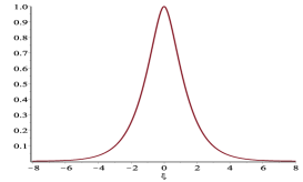
Figure 1: The single pseudo-peakon solution (36)

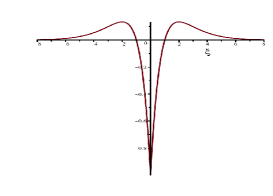
Figure 2: The peaked second derivative (37)

We can also compute multi-pseudo-peakon solutions. They are of the form

$$u=\sum_{j=1}^{N}\frac{p_{j}(t)}{2}e^{-|x-q_{j}(t)|}(1+|x-q_{j}(t)|)\;,$$ (38)

where $p_{j}(t),\ q_{j}(t)$ satisfy the following canonical Hamiltonian dynamical system

$$\dot{q}_{j} = \frac{\partial H}{\partial p_{j}},$$ (39)

$$\dot{p}_{j} = -\frac{\partial H}{\partial q_{j}},$$ (40)

with Hamiltonian function:

$$H = \frac{1}{2}\sum_{i,j=1}^{N}p_{i}p_{j}e^{-|q_{i}-q_{j}|}\;.$$ (41)

A crucial observation is that (39)–(41) coincides exactly with the finite-dimensional peakon dynamical system of the CH equation, see [5]. As we will explain momentarily, this fact allows us to have a full picture of multi-pseudo-peakon solutions. First, let us calculate explicitly $2$-pseudo-peakons. When $N=2$, we have the $2-$pseudo-peakon equations below:

$$\left\{\begin{array}[]{l}p_{1,t}=p_{1}p_{2}\,{\rm sgn}(q_{1}-q_{2})\,e^{-|q_{1}-q_{2}|}\;,\\ p_{2,t}=p_{1}p_{2}\,{\rm sgn}(q_{2}-q_{1})\,e^{-|q_{1}-q_{2}|}\;,\\ q_{1,t}=p_{1}+p_{2}\,e^{-|q_{1}-q_{2}|}\;,\\ q_{2,t}=p_{2}+p_{1}\,e^{-|q_{1}-q_{2}|}\;,\end{array}\right.$$ (46)

which can be solved with the following explicit solutions:

$$\left\{\begin{array}[]{l}p_{1}(t)=-p_{2}(t)=A\coth(At),\\ q_{1}(t)=-q_{2}(t)=\ln\cosh(At),\end{array}\right.$$ (49)

where $A$ is an arbitrary constant. Thus, the 2-pseudo-peakon solution of the fifth order CH-type equation (10) is given by

$$u(x,t) = \frac{p_{1}(t)}{2}e^{-|x-q_{1}(t)|}(1+|x-q_{1}(t)|)+\frac{p_{2}(t)}{2}e^{-|x-q_{2}(t)|}(1+|x-q_{2}(t)|)$$

$$= \frac{A}{2}\coth(At)\left[e^{-|x-\ln\cosh(At)|}(1+|x-\ln\cosh(At)|)-e^{-|x+\ln\cosh(At)|}(1+|x+\ln\cosh(At)|)\right],$$

where $\cosh(At)=\frac{e^{At}+e^{-At}}{2}$, and $\coth(At)=\frac{e^{At}+e^{-At}}{e^{At}-e^{-At}}$. If we fix time $t=\frac{\cosh^{-1}e}{A}$ and we select $A=\frac{2}{\coth(\cosh^{-1}e)}$, the above 2-pseudo-peakon solution reads as the following simplest form

$$u(x,t) = e^{-|x-1|}(1+|x-1|)-e^{-|x+1|}(1+|x+1|),$$

which we may plot in a 2D picture for the two pseudo-peakon interaction (see Figure 4).

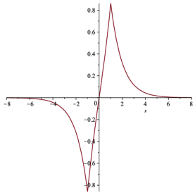
Figure 3: The two pseudo-peakon interaction plotted in 3D for negative time $t$.

Figure 4: The two pseudo-peakon interaction plotted in 3D for all times.

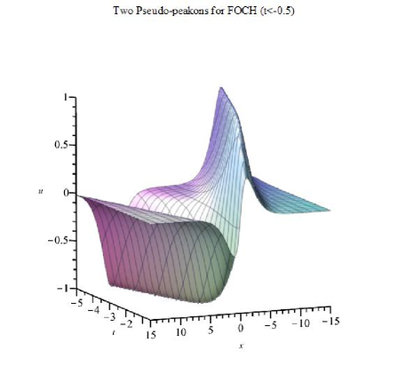
Figure 5: The two pseudo-peakon interaction plotted in 3D for negative time $t$.

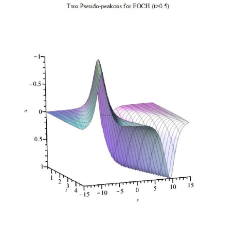
Figure 6: The two pseudo-peakon interaction plotted in 3D for positive time $t$.

Remark 5.

The plots below show $2$-pseudo-peakons in 3D. Figure 4 shows a 3D interactional dynamics of the $2$-pseudo-peakon solution for all times. Figure 6 and Figure 6 show a 3D interactional dynamics of the two-pseudo-peakon solution for the negative times and the positive times, respectively. During the interaction of two-pseudo-peakons, it follows from the explicit solution (LABEL:2-Pseudo-Peakon-u) that the solution $u$ suddenly crashes to zero when the time $t$ passes from negative to positive via $t=0$. After the time $t=0$, the two-pseudo-peakon solution continues travelling from left to right, but the amplitudes already flipped along with the time (see Figure 6 and Figure 6 for details).

Now we consider multi-pseudo-peakons in full generality. It is known that the Hamiltonian system (39)–(41) —that in our context will be called the multi-pseudo-peakon system— is completely integrable in the Liouville sense. This fact is discussed in [5] and fully studied by Calogero and Françoise in [4]. Since the Hamiltonian (41) is not continuously differentiable, we cannot conclude that the trajectories of the system are given by quadratures via the Arnold-Liouville theorem. However, in the papers [2, 3] Beals, Sattinger and Szmigielski are able to solve the Hamiltonian system (39)–(41) via inverse spectral methods and continued fractions. More precisely we have, after the summary appearing in [6, Theorem 2.1]:

Theorem 4.

The solutions of the Hamiltonian system

$$\frac{dx_{j}}{d\tau}=\frac{\partial H}{\partial m_{j}}\;,\quad\;\frac{dm_{j}}{d\tau}=-\frac{\partial H}{\partial x_{j}}\;,\quad\;H(x_{1},\cdots,x_{N},m_{1},\cdots,m_{N})=\frac{1}{4}\sum_{j,k=1}^{N}m_{j}m_{k}e^{-2|x_{j}-x_{k}|}$$ (51)

are given by

$$x_{j}=\frac{1}{2}\log\left(\frac{1+y_{j}}{1-y_{j}}\right)\;,\quad\quad\quad m_{j}=g_{j}(1-y_{j}^{2})\;,$$ (52)

in which

$$y_{j}=1-\frac{\Delta_{N-j}^{2}}{\Delta_{N-j+1}^{0}}\;,\quad\quad\quad g_{j}=\frac{(\Delta_{N-j+1}^{0})^{2}}{\Delta_{N-j+1}^{1}\,\Delta_{N-j}^{1}}\;.$$

The functions $\Delta_{k}^{l}(\tau)$ are given by

$$\Delta_{k}^{l}=\det(A_{i+j+l}(\tau))_{i,j=1}^{k-1}\;,\quad\quad A_{k}(\tau)=\sum_{j=0}^{N}(-\lambda_{j})^{k}\,a_{j}(\tau)\;,\quad a_{0}(\tau)=\frac{1}{2}\;,\quad\lambda_{0}=0\;,$$

with $\frac{d}{d\tau}a_{j}(\tau)=-\frac{2a_{j}(\tau)}{\lambda_{j}}$ and $\lambda_{j}\neq 0$ for $j\geq 1$.

In this theorem we assume that the numbers $\lambda_{j}$ are all distinct and have the same sign, and that the initial conditions $a_{j}(0)$ are positive, see [6, p. 158].

Now, in order to obtain solutions to the system (39)–(41), we apply the symplectic transformation $x_{j}\mapsto(1/2)\,q_{j}$, $m_{j}\mapsto 2p_{j}$. Then, the Hamiltonian appearing in (51) becomes (41), and trajectories of (51) map onto trajectories of (39)–(41). We adjust the time evolution by setting $t=2\tau$ and we are ready: replacing $q_{j}(t)$ and $p_{j}(t)$ into our formula (38) we obtain explicit expressions for $N$-pseudo-peakons.

4 The Cauchy problem for the CH-type equation

In this section we consider the Cauchy problem for the fifth order CH-type equation (10). We rewrite (10) as

$$\left\{\begin{array}[]{ll}m_{t}+2\,(u-u_{xx})_{x}\,m+(u-u_{xx})\,m_{x}=0,\\ m=-A_{4}(u)=(1-\partial_{x}^{2})^{2}u=u-2u_{xx}+u_{xxxx}\;.\end{array}\right.$$ (55)

The operator $(1-\partial_{x}^{2})^{-2}$ can be expressed by

$$(1-\partial_{x}^{2})^{-2}f=G*f=\int_{{\mathbb{R}}}G(x-y)f(y)dy$$

for any $f\in L^{2}({\mathbb{R}})$ with $G=\frac{1}{4}(1+|x|)e^{-|x|}$. It follows

$$u(x,t) = G*m=\frac{1}{4}\int_{\mathbb{R}}(1+|x-\xi|)e^{-|x-\xi|}m(\xi,t)d\xi$$

$$= \frac{1}{4}e^{-x}\int_{-\infty}^{x}(1+x-\xi)e^{\xi}m(\xi,t)d\xi+\frac{1}{4}e^{x}\int_{x}^{+\infty}(1-x+\xi)e^{-\xi}m(\xi,t)d\xi.$$

Then,

$$u_{x}(x,t) = -\frac{1}{4}e^{-x}\int_{-\infty}^{x}(1+x-\xi)e^{\xi}m(\xi,t)d\xi+\frac{1}{4}e^{x}\int_{x}^{+\infty}(1-x+\xi)e^{-\xi}m(\xi,t)d\xi$$

$$+\frac{1}{4}e^{-x}\int_{-\infty}^{x}e^{\xi}m(\xi,t)d\xi-\frac{1}{4}e^{x}\int_{x}^{+\infty}e^{-\xi}m(\xi,t)d\xi$$

and

$$u_{xx}(x,t) = \frac{1}{4}e^{-x}\int_{-\infty}^{x}(1+x-\xi)e^{\xi}m(\xi,t)d\xi+\frac{1}{4}e^{x}\int_{x}^{+\infty}(1-x+\xi)e^{-\xi}m(\xi,t)d\xi$$ (57)

$$-\frac{1}{2}e^{-x}\int_{-\infty}^{x}e^{\xi}m(\xi,t)d\xi-\frac{1}{2}e^{x}\int_{x}^{+\infty}e^{-\xi}m(\xi,t)d\xi.$$

(4) minus (57), we have

$$(u-u_{xx})(x,t)=\frac{1}{2}e^{-x}\int_{-\infty}^{x}e^{\xi}m(\xi,t)d\xi+\frac{1}{2}e^{x}\int_{x}^{+\infty}e^{-\xi}m(\xi,t)d\xi.$$ (58)

Differentiating $u-u_{xx}$ with respect to $x$, we have

$$(u_{x}-u_{xxx})(x,t)=-\frac{1}{2}e^{-x}\int_{-\infty}^{x}e^{\xi}m(\xi,t)d\xi+\frac{1}{2}e^{x}\int_{x}^{+\infty}e^{-\xi}m(\xi,t)d\xi.$$ (59)

4.1 Local well-posedness and blow-up scenario

Firstly, we present the local well-posedness theorem for the CH type equation (55).

Theorem 5.

Let $u_{0}\in H^{s}(\mathbb{R})$ with $s>\frac{7}{2}$. Then there exist a $T>0$ depending on $\|u_{0}\|_{H^{s}}$, such that the CH type equation (55) has a unique solution

$$u\in C([0,T);H^{s}(\mathbb{R}))\cap C^{1}([0,T);H^{s-1}(\mathbb{R})).$$

Morever, the map $u_{0}\in H^{s}\rightarrow u\in C([0,T);H^{s}(\mathbb{R}))\cap C^{1}([0,T);H^{s-1}(\mathbb{R}))$ is continuous.

The proof (via Kato’s theory) is similar to the ones appearing in [11] and [29, Section 3], and therefore we have omitted the details. The maximum value of $T$ appearing in Theorem 5 is called the lifespan of the solution. If $T<\infty$, that is,

$$\lim_{t\to T^{-}}\|u\|_{H^{s}}=\infty\;,$$

we say the solution blows up in finite time. Now we can use one of the conserved densities found in Section 2, namely, the Hamiltonian (34). We have

$$\int_{{\mathbb{R}}}(u^{2}+3u_{x}^{2}+3u_{xx}^{2}+u_{xxx}^{2})dx=\int_{{\mathbb{R}}}(u_{0}^{2}+3u_{0x}^{2}+3u_{0xx}^{2}+u_{0xxx}^{2})dx:=E_{0}^{2}\;.$$ (60)

We note that

$$\|u_{x}\|_{L^{\infty}}\leq\frac{\|u_{x}\|_{H^{1}}}{\sqrt{2}}\leq\frac{E_{0}}{\sqrt{2}}\;.$$

This means that the first-order derivative of $u$ is always bounded. Let us present the precise blow-up scenario.

Theorem 6.

Assume that $u_{0}\in H^{4}(\mathbb{R})$ and let $T$ be the maximal existence time of the solution $u(x,t)$ to the CH type equation (55) with the initial data $u_{0}(x)$, then the corresponding solution of the CH type equation (55) blows up in finite time if and only if

$$\lim_{t\to T}\sup_{x\in{\mathbb{R}}}\{(u_{xxx})(x,t)\}=\infty.$$

Remark 6.

This theorem means that the blow-up mechanism of (55) is not the same as in the CH case: for the CH equation, see [11, 12], blow-up phenomenon means that the first-order derivative tends to negative infinity. However, for our equation blow-up means that the third-order derivative tends to infinity.

Proof.

By direct calculation, we have

$$\|u\|_{H^{4}}^{2}\leq\|m\|_{L^{2}}^{2}\leq 3\|u\|_{H^{4}}^{2}\;.$$

Multiplying (55) by $m$, we obtain by straighforward computations,

$$\frac{d}{dt}\int_{\mathbb{R}}m^{2}dx = -2\int_{\mathbb{R}}2\,(-u_{xx}+u)_{x}\,m^{2}+(-u_{xx}+u)\,m_{x}\,mdx$$

$$\leq -3\inf_{x\in{\mathbb{R}}}\{u_{x}-u_{xxx}\}\int_{\mathbb{R}}m^{2}dx$$

$$\leq {\color[rgb]{0,0,0}\left(\frac{3}{\sqrt{2}}E_{0}+3\sup_{x\in{\mathbb{R}}}\{u_{xxx}\}\right)\int_{\mathbb{R}}m^{2}dx.}$$

If

$$\sup_{x\in{\mathbb{R}}}\{u_{xxx}\}\leq M,$$

then

$$\frac{d}{dt}\int_{\mathbb{R}}m^{2}dx\leq{\color[rgb]{0,0,0}\left(\frac{3}{\sqrt{2}}E_{0}+3M\right)}\int_{\mathbb{R}}m^{2}dx.$$

By using the Gronwall inequality,

$$\|m\|_{L^{2}}^{2}\leq e^{{\color[rgb]{0,0,0}\left(\frac{3}{\sqrt{2}}E_{0}+3M\right)}}\|m_{0}\|_{L^{2}}^{2}.$$

Therefore the $H^{4}$-norm of the solution is bounded on $[0,T)$. On the other hand, by the Sobolev’s embedding $\|u_{xxx}\|_{L^{\infty}}\leq\|u\|_{H^{4}}$. This inequality tells us that if $H^{4}$-norm of the solution is bounded, then the $L^{\infty}$-norm of $u_{xxx}$ is bounded. We have completed the proof of Theorem 6. ∎

4.2 Global existence and blow up phenomena

In this subsection, firstly, we establish a sufficient condition that guarantees global existence of the solution to our CH type equation (55). We give the particle trajectory as

$$\left\{\begin{array}[]{ll}q_{t}(x,t)=(u-u_{xx})(q(x,t),t),\qquad 0<t<T,x\in\mathbb{R},\\ q(x,0)=x,\qquad x\in\mathbb{R},\end{array}\right.$$ (63)

where $T$ is the lifespan of the solution. Taking derivative of (63) with respect to $x$, we obtain

$$\frac{dq_{t}(x,t)}{dx}=q_{tx}=((u_{x}-u_{xxx})q_{x})(q(x,t),t),\qquad t\in(0,T).$$

Therefore

$$\left\{\begin{array}[]{ll}q_{x}=exp\{\int^{t}_{0}(u_{x}-u_{xxx})(q,s)ds\},\quad 0<t<T,\quad x\in\mathbb{R},\\ q_{x}(x,0)=1,\qquad x\in\mathbb{R},\end{array}\right.$$

which is always positive before the blow-up time. Therefore, the function $q(x,t)$ is an increasing diffeomorphism of the line before blow-up. In fact, direct calculation yields

$$\frac{d}{dt}(m(q(x,t),t)q^{b}_{x})=[m_{t}(q)+(u_{x}-u_{xxx})(q,t)m_{x}(q)+2(u_{x}-u_{xxx})(q,t)m(q)]q^{2}_{x}=0.$$

Hence, the following identity can be proved:

$$m(q(x,t),t)q^{2}_{x}=m_{0}(x),\qquad 0<t<T,x\in\mathbb{R}.$$ (65)

From (65), we know that if the initial data $m_{0}(x,t)\geq 0$, then $m(q(x_{0},t),t)\geq 0$. Before stating our main results, we recall once again the useful conservation law

$$\int_{{\mathbb{R}}}(u^{2}+3u_{x}^{2}+3u_{xx}^{2}+u_{xxx}^{2})dx=\int_{{\mathbb{R}}}(u_{0}^{2}+3u_{0x}^{2}+3u_{0xx}^{2}+u_{0xxx}^{2})dx:=E_{0}^{2}$$ (66)

found in Section 2.

Theorem 7.

Suppose that $u_{0}\in H^{4}({\mathbb{R}})$, and $m_{0}=(1-\partial_{x}^{2})^{2}u_{0}$ does not change sign. Then the corresponding solution to the CH-type equation (55) exists globally.

Proof.

From (65), we known that $m(x,t)$ does not change sign either. By Theorem 6, we only need to bound $u_{xxx}(x,t)$ from above. Now, we already observed that $u_{x}$ is always bounded thanks to the conservation law (66). It follows that if we can bound $u_{x}-u_{xxx}$ from below, we will have our proof.

For $m_{0}\geq 0$, by (58) and (59), we obtain

$$(u_{x}-u_{xxx})(x,t)+(u-u_{xx})(x,t)=e^{x}\int_{x}^{+\infty}e^{-\xi}m(\xi,t)d\xi\geq 0.$$

It follows

$$(u_{x}-u_{xxx})(x,t)\geq-(u-u_{xx})(x,t)$$

$$\geq-\left(\int_{{\mathbb{R}}}u^{2}+3u_{x}^{2}+3u_{xx}^{2}+u_{xxx}^{2}dx\right)^{\frac{1}{2}}=-E_{0}.$$

Similarly, for $m_{0}\leq 0$, we have

$$(u_{x}-u_{xxx})(x,t)\geq(u-u_{xx})(x,t)\geq-E_{0}.$$

The proof of Theorem 7 is completed. ∎

Theorem 8.

Suppose that $u_{0}\in H^{4}({\mathbb{R}})$, and that there exists $x_{0}\in{\mathbb{R}}$ such that $m_{0}(x)\leq 0$ on $(-\infty,x_{0}]$ and $m_{0}(x)\geq 0$ on $[x_{0},\infty)$. Then the corresponding solution to the CH-type equation (55) exists globally.

Proof.

Similarly to the argument in the proof of Theorem 7, we need to bound $u_{x}-u_{xxx}$ from below. From (65), we known that $m(x,t)\leq 0$ on $(-\infty,q(x_{0},t)]$ and $m(x,t)\geq 0$ on $[q(x_{0},t),\infty)$. For the points $x\in(-\infty,q(x_{0},t)]$, we have

$$(u_{x}-u_{xxx})(x,t)=(u-u_{xx})(x,t)-e^{-x}\int_{-\infty}^{x}e^{\xi}m(\xi,t)d\xi\geq(u-u_{xx})(x,t).$$

For the points $x\in[q(x_{0},t),\infty)$, we have

$$(u_{x}-u_{xxx})(x,t)=-(u-u_{xx})(x,t)+e^{x}\int_{x}^{+\infty}e^{-\xi}m(\xi,t)d\xi\geq-(u-u_{xx})(x,t).$$

This means that for any $x\in{\mathbb{R}}$ we have

$$(u_{x}-u_{xxx})(x,t)\geq-\|u-u_{xx}\|_{L^{\infty}}\geq-E_{0},$$

where we have used the conservation law (66) once again. We have completed the proof of Theorem 8. ∎

Theorem 9.

Assume that $u_{0}\in H^{4}(\mathbb{R})$ and that there exists $x_{0}\in{\mathbb{R}}$ such that

$$(u_{0x}-u_{0xxx})(x_{0})<-\frac{E_{0}}{\sqrt{2}}\;,$$ (67)

where $E_{0}$ is defined in (66). Then, the corresponding solution $u(x,t)$ to CH type equation (55) blows up at a finite time $T$ bounded by

$$T\leq\frac{1}{-\frac{1}{2}(u_{0x}-u_{0xxx})(x_{0})+\frac{E_{0}^{2}}{2(u_{0x}-u_{0xxx})(x_{0})}}\;.$$

Remark 7.

Due to the fact that $u_{0x}$ is bounded by the conservation law $E_{0}$ with $\|u_{0x}\|_{L^{\infty}}\leq\frac{\|u_{0x}\|_{H^{1}}}{\sqrt{2}}\leq\frac{E_{0}}{\sqrt{2}}$, the condition (67) holds true only if $u_{0xxx}(x_{0})>\sqrt{2}E_{0}$.

Proof.

Let

$$I(t)=\frac{1}{2}e^{-q(x_{0},t)}\int_{-\infty}^{q(x_{0},t)}e^{x}m(x,t)dx$$

and

$$II(t)=\frac{1}{2}e^{q(x_{0},t)}\int_{q(x_{0},t)}^{+\infty}e^{-x}m(x,t)dx.$$

From (58) and (59), we have

$$(u-u_{xx})(q(x_{0},t),t)=I(t)+II(t)$$

and

$$(u_{x}-u_{xxx})(q(x_{0},t),t)=-I(t)+II(t).$$

Differentiating $(u_{x}-u_{xxx})(q(x_{0},t),t)$ with respect to $t$,

$$\frac{d}{dt}(u_{x}-u_{xxx})(q(x_{0},t),t)=-\frac{d}{dt}I(t)+\frac{d}{dt}II(t).$$ (68)

Then, we estimate $\frac{d}{dt}I(t)$.

$$\frac{d}{dt}I(t) = \frac{1}{2}(u-u_{xx})m(q(x_{0},t),t)-\frac{1}{2}(u-u_{xx})e^{-q(x_{0},t)}\int_{-\infty}^{q(x_{0},t)}e^{x}m(x,t)dx$$

$$+\frac{1}{2}e^{-q(x_{0},t)}\int_{-\infty}^{q(x_{0},t)}e^{x}m_{t}(x,t)dx.$$

The third term in the right hand side can been estimated as

$$\frac{1}{2}e^{-q(x_{0},t)}\int_{-\infty}^{q(x_{0},t)}e^{x}m_{t}(x,t)dx$$

$$= -\frac{1}{2}e^{-q(x_{0},t)}\int_{-\infty}^{q(x_{0},t)}e^{x}((u-u_{xx})m_{x}+2(u-u_{xx})_{x}m)(x,t)dx$$

$$= -\frac{1}{2}e^{-q(x_{0},t)}\int_{-\infty}^{q(x_{0},t)}e^{x}(((u-u_{xx})m)_{x}+(u-u_{xx})_{x}m)(x,t)dx$$

$$= -\frac{1}{2}(u-u_{xx})m(q(x_{0},t),t)+\frac{1}{2}e^{-q(x_{0},t)}\int_{-\infty}^{q(x_{0},t)}e^{x}(((u-u_{xx})m)-(u-u_{xx})_{x}m)(x,t)dx$$

$$= -\frac{1}{2}(u-u_{xx})m(q(x_{0},t),t)+\frac{1}{2}e^{-q(x_{0},t)}\int_{-\infty}^{q(x_{0},t)}e^{x}\left((u-u_{xx})^{2}-(u-u_{xx})(u-u_{xx})_{xx}\right.$$

$$\left.-(u-u_{xx})_{x}(u-u_{xx})+(u-u_{xx})_{x}(u-u_{xx})_{xx}\right)dx$$

$$= -\frac{1}{2}(u-u_{xx})m(q(x_{0},t),t)-\frac{1}{2}(u-u_{xx})(u-u_{xx})_{x}+\frac{1}{4}(u-u_{xx})_{x}^{2}$$

$$+\frac{1}{2}e^{-q(x_{0},t)}\int_{-\infty}^{q(x_{0},t)}e^{x}\left((u-u_{xx})^{2}+\frac{1}{2}(u-u_{xx})_{x}^{2}\right)dx.$$

It follows that

$$\frac{d}{dt}I(t) = -\frac{1}{2}(u-u_{xx})e^{-q(x_{0},t)}\int_{-\infty}^{q(x_{0},t)}e^{x}m(x,t)dx-\frac{1}{2}(u-u_{xx})(u-u_{xx})_{x}+\frac{1}{4}(u-u_{xx})_{x}^{2}$$

$$+\frac{1}{2}e^{-q(x_{0},t)}\int_{-\infty}^{q(x_{0},t)}e^{x}\left((u-u_{xx})^{2}+\frac{1}{2}(u-u_{xx})_{x}^{2}\right)dx$$

$$= -\frac{1}{2}(u-u_{xx})^{2}+\frac{1}{4}(u-u_{xx})_{x}^{2}+\frac{1}{2}e^{-q(x_{0},t)}\int_{-\infty}^{q(x_{0},t)}e^{x}\left((u-u_{xx})^{2}+\frac{1}{2}(u-u_{xx})_{x}^{2}\right)dx.$$

Note that

$$\int_{-\infty}^{q(x_{0},t)}e^{x}\left((u-u_{xx})^{2}+(u-u_{xx})_{x}^{2}\right)dx$$

$$\geq 2\int_{-\infty}^{q(x_{0},t)}e^{x}(u-u_{xx})(u-u_{xx})_{x}dx$$

$$\geq e^{q(x_{0},t)}(u-u_{xx})^{2}(q(x_{0},t),t)-\int_{-\infty}^{q(x_{0},t)}e^{x}(u-u_{xx})^{2}dx,$$

which yields that

$$\int_{-\infty}^{q(x_{0},t)}e^{x}\left((u-u_{xx})^{2}+\frac{1}{2}(u-u_{xx})_{x}^{2}\right)dx\geq\frac{1}{2}e^{q(x_{0},t)}(u-u_{xx})^{2}(q(x_{0},t),t).$$

Therefore,

$$\frac{d}{dt}I(t)\geq-\frac{1}{4}(u-u_{xx})^{2}(q(x_{0},t),t)+\frac{1}{4}(u-u_{xx})_{x}^{2}(q(x_{0},t),t).$$ (69)

Similarity,

$$\frac{d}{dt}II(t) = -\frac{1}{2}(u-u_{xx})m(q(x_{0},t),t)+\frac{1}{2}(u-u_{xx})e^{q(x_{0},t)}\int_{q(x_{0},t)}^{+\infty}e^{-x}m(x,t)dx$$

$$+\frac{1}{2}e^{q(x_{0},t)}\int_{q(x_{0},t)}^{+\infty}e^{-x}m_{t}(x,t)dx.$$

The third term in the right hand side can been estimated as

$$\frac{1}{2}e^{q(x_{0},t)}\int_{q(x_{0},t)}^{+\infty}e^{-x}m_{t}(x,t)dx$$

$$= \frac{1}{2}(u-u_{xx})m(q(x_{0},t),t)-\frac{1}{2}(u-u_{xx})(u-u_{xx})_{x}-\frac{1}{4}(u-u_{xx})_{x}^{2}$$

$$-\frac{1}{2}e^{q(x_{0},t)}\int_{q(x_{0},t)}^{\infty}e^{-x}\left((u-u_{xx})^{2}+\frac{1}{2}(u-u_{xx})_{x}^{2}\right)dx.$$

It follows that

$$\frac{d}{dt}II(t) = \frac{1}{2}(u-u_{xx})e^{q(x_{0},t)}\int_{q(x_{0},t)}^{+\infty}e^{-x}m(x,t)dx$$

$$-\frac{1}{2}(u-u_{xx})(u-u_{xx})_{x}-\frac{1}{4}(u-u_{xx})_{x}^{2}$$

$$-\frac{1}{2}e^{q(x_{0},t)}\int_{q(x_{0},t)}^{\infty}e^{-x}\left((u-u_{xx})^{2}+\frac{1}{2}(u-u_{xx})_{x}^{2}\right)dx.$$

By same argument, we have

$$\int_{q(x_{0},t)}^{\infty}e^{-x}\left((u-u_{xx})^{2}+\frac{1}{2}(u-u_{xx})_{x}^{2}\right)dx\geq\frac{1}{2}e^{-q(x_{0},t)}(u-u_{xx})^{2}(q(x_{0},t),t).$$

Therefore

$$\frac{d}{dt}II(t)\leq\frac{1}{4}(u-u_{xx})^{2}(q(x_{0},t),t)-\frac{1}{4}(u-u_{xx})_{x}^{2}(q(x_{0},t),t).$$ (70)

Inserting (69) and (70) into (68), we have

$$\frac{d}{dt}(u_{x}-u_{xxx})(q(x_{0},t),t)$$ (71)

$$= (u-u_{xx})^{2}(q(x_{0},t),t)-\frac{1}{2}(u-u_{xx})_{x}^{2}(q(x_{0},t),t)$$

$$-\frac{1}{2}e^{-q(x_{0},t)}\int_{-\infty}^{q(x_{0},t)}e^{x}\left((u-u_{xx})^{2}+\frac{1}{2}(u-u_{xx})_{x}^{2}\right)dx$$

$$-\frac{1}{2}e^{q(x_{0},t)}\int_{q(x_{0},t)}^{\infty}e^{-x}\left((u-u_{xx})^{2}+\frac{1}{2}(u-u_{xx})_{x}^{2}\right)dx.$$

Combining the above estimates into (71), we obtain

$$\frac{d}{dt}(u_{x}-u_{xxx})(q(x_{0},t),t)\leq\frac{1}{2}(u-u_{xx})^{2}(q(x_{0},t),t)-\frac{1}{2}(uu_{xx})_{x}^{2}(q(x_{0},t),t).$$ (72)

By the fact $\|f\|_{L^{\infty}}^{2}<\frac{1}{2}\|f\|_{H^{1}}^{2}$, we have

$$\|u-u_{xx}\|_{L^{\infty}}^{2}<\frac{1}{2}\|u-u_{xx}\|_{H^{1}}^{2}=\frac{1}{2}E_{0}^{2}.$$

Let $\varphi(t)=(u_{x}-u_{xxx})(q(x_{0},t),t)$, we can rewrite (72) as

$$\varphi^{\prime}(t)\leq-\frac{1}{2}\varphi^{2}(t)+\frac{1}{4}E_{0}^{2}.$$

By using the hypothesis of the theorem and a standard argument on Riccati type equations, we have that there exists a time $T$ such that

$$\lim_{t\rightarrow T}\varphi(t)=-\infty.$$

By the boundedness of $u_{x}$, we have that $u_{xxx}$ goes to infinity. This completes the proof of Theorem 9. ∎

Theorem 10.

Assume that $u_{0}\in H^{4}(\mathbb{R})$ and that there exists $x_{0}\in{\mathbb{R}}$ such that $m_{0}(x_{0})=(1-\partial_{x}^{2})^{2}u_{0}(x_{0})=0$,

$$\int_{-\infty}^{x_{0}}e^{x}m_{0}(x,t)dx>0\quad\mathrm{and}\quad\int_{x_{0}}^{\infty}e^{-x}m_{0}(x,t)dx<0,$$ (73)

then the corresponding solution $u(x,t)$ to CH type equation (55) blows up in finite time.

Proof.

Thanks to (65), we obtain $m(q(x_{0},t),t)=0$ for all $t$ in its lifespan. Inequality (72) is also correct in this proof. The initial condition (73) means that $(u_{0}-u_{0xx})_{x}(q(x_{0},t),t)<0$ and $(u_{0}-u_{0xx})_{x}^{2}(x_{0},t)>(u_{0}-u_{0xx})^{2}(q(x_{0},t),t)$. We claim that $(u_{0}-u_{0xx})_{x}(q(x_{0},t),t)$ is decreasing, $(u-u_{xx})_{x}^{2}(q(x_{0},t),t)>(u-u_{xx})^{2}(q(x_{0},t),t)$ for all $t\geq 0$. Suppose not, i.e. there exists a $t_{0}$ such that $(u-u_{xx})_{x}^{2}(q(x_{0},t),t)>(u-u_{xx})^{2}(q(x_{0},t),t)$ on $[0,t)$ and $(u-u_{xx})_{x}^{2}(q(x_{0},t_{0}),t_{0})\leq(u-u_{xx})^{2}(q(x_{0},t_{0}),t_{0})$. Recall (69) and (70), we get on $[0,t_{0})$

$$\frac{d}{dt}I(t)\geq-\frac{1}{4}(u-u_{xx})^{2}(q(x_{0},t),t)+\frac{1}{4}(u-u_{xx})_{x}^{2}(q(x_{0},t),t)\geq 0$$

and

$$\frac{d}{dt}II(t)\leq\frac{1}{4}(u-u_{xx})^{2}(q(x_{0},t),t)-\frac{1}{4}(u-u_{xx})_{x}^{2}(q(x_{0},t),t)\leq 0.$$

It follows from the continuity property of ODEs that

$$(u-u_{xx})^{2}(q(x_{0},t),t)-(u-u_{xx})_{x}^{2}(q(x_{0},t),t)=4I(t)II(t)<4I(0)II(0)<0,$$

for all $t>0$, this implies that $t_{0}$ can be extended to the infinity. This is a contradiction. So the claim is true. By using (69) and (70) again, we get

$$\frac{d}{dt}[(u-u_{xx})_{x}^{2}-(u-u_{xx})^{2}](q(x_{0},t),t)$$ (74)

$$= -\frac{d}{dt}\left\{\int_{-\infty}^{q(x_{0},t)}e^{x}m(x,t)dx\times\int_{q(x_{0},t)}^{+\infty}e^{-x}m(x,t)dx\right\}$$

$$= -4\frac{d}{dt}[I(t)II(t)]$$

$$= -4\frac{d}{dt}I(t)\times II(t)-4\frac{d}{dt}II(t)\times I(t)$$

$$\geq -[(u-u_{xx})_{x}^{2}-(u-u_{xx})^{2}](q(x_{0},t),t)II(t)+[(u-u_{xx})_{x}^{2}-(u-u_{xx})^{2}](q(x_{0},t),t)I(t)$$

$$= -(u-u_{xx})_{x}(q(x_{0},t),t)[(u-u_{xx})_{x}^{2}-(u-u_{xx})^{2}](q(x_{0},t),t),$$

where we have used $(u-u_{xx})_{x}(q(x_{0},t),t)=-I(t)+II(t)$. Recall (72), it follows

$$(u_{x}-u_{xxx})(q(x_{0},t),t)$$

$$\leq \int_{0}^{t}\frac{1}{2}[(u-u_{xx})^{2}(q(x_{0},s),s)-(u-u_{xx})_{x}^{2}(q(x_{0},s),s)]ds-(u_{x}-u_{xxx})(x_{0},0).$$

Substituting (4.2) into (74), it yields

$$\frac{d}{dt}[(u-u_{xx})_{x}^{2}-(u-u_{xx})^{2}](q(x_{0},t),t)\geq\frac{1}{2}[(u-u_{xx})_{x}^{2}-(u-u_{xx})^{2}](q(x_{0},t),t)$$

$$\times\left\{\int_{0}^{t}[(u-u_{xx})_{x}^{2}-(u-u_{xx})^{2}](q(x_{0},s),s)ds+2(u_{x}-u_{xxx})(x_{0},0)\right\}.$$

Before completing the proof, we need the following technical lemma.

Lemma 1.

[32] Suppose that $\Psi(t)$ is twice continuously differentiable satisfying

$$\left\{\begin{array}[]{ll}\Psi^{\prime\prime}(t)\geq C_{0}\Psi^{\prime}(t)\Psi(t),\quad t>0,\quad C_{0}>0,\\ \Psi(t)>0,\quad\Psi^{\prime}(t)>0.\end{array}\right.$$ (79)

Then $\Psi(t)$ blows up in finite time. Moreover, the blow up time can be estimated in terms of the initial datum as

$$T\leq\max\left\{\frac{2}{C_{0}\Phi(0),\frac{\Phi(0)}{\Phi^{\prime}(0)}}\right\}.$$

Let $\Psi(t)=\int_{0}^{t}[(u-u_{xx})_{x}^{2}-(u-u_{xx})^{2}](q(x_{0},s),s)ds+2(u_{x}-u_{xxx})(x_{0},0)$, then (4.2) is an equation of type (79) with $C_{0}=\frac{1}{2}$. The proof is completed by applying Lemma 1 and the boundedness of $u_{x}$. ∎

5 Final Remarks

In this final section we collect three different remarks: first, we introduce some $(2n+1)th$ order CH-type equations, $n\geq 1$; second, we discuss the relation of these equations with the geometry of the diffeomorphism group $Diff(S^{1})$; third, we reconnect our class of equations with the geometry of pseudo-spherical surfaces.

5.1 Higher order Camassa-Holm type equations

In this subsection we proceed as in Section 2. We consider differential operators $A_{2n}$ of order $2n$ and define $m=A_{2n}(u)$. Specifically, we choose the operators

$$A_{2n} = (-1)^{n+1}\partial_{x}^{2n}+2\sum_{k=1}^{n-1}(-1)^{n+1-k}\,\partial_{x}^{2(n-k)}-1\;,$$ (80)

$$B_{2n} = \sum_{k=0}^{n-1}(-1)^{n-k}\,\partial_{x}^{2(n-k)-1}\;,$$

$$C_{2n} = \sum_{k=0}^{n-1}(-1)^{n-k}\,\partial_{x}^{2(n-k-1)}\;.$$

We consider the matrices

$$X_{2n}=\left[\begin{array}[]{cc}0&\frac{1}{2}\,\lambda+A_{2n}(u)\\ \vskip 6.0pt plus 2.0pt minus 2.0pt\cr\frac{1}{2}\,{\lambda}^{-1}&0\end{array}\right]$$ (81)

and

$$T_{2n}=\left[\begin{array}[]{cc}\frac{1}{2}\,B_{2n}(u)&C_{2n}(u)\,A_{2n}(u)-\frac{1}{2}\,\lambda\,C_{2n}(u)-\frac{1}{2}\,\lambda^{2}\\ \vskip 6.0pt plus 2.0pt minus 2.0pt\cr\displaystyle-\frac{1}{2}+\frac{1}{2\lambda}\,C_{2n}(u)&-\frac{1}{2}\,B_{2n}(u)\end{array}\right]\;.$$ (82)

A straightforward computation allows us to check that the equation

$$X_{2n,t}-T_{2n,x}+[X_{2n},T_{2n}]=0$$

is equivalent to the $(2n+1)$-order equation of Camassa-Holm type

$$A_{2n,t}(u)-2\,C_{2n}(u)_{x}\,A_{2n}(u)-C_{2n}(u)\,A_{2n}(u)_{x}=0\;.$$ (83)

It follows from our discussions in Section 1 and [9] that these equations all describe pseudo-spherical surfaces. We compute quadratic pseudo-potentials and conservation laws as in Section 2: we obtain the Riccati equation

$${\frac{\partial\Gamma}{\partial x}}=\frac{1}{2}\,\lambda+A_{2n}(u)-{\frac{\Gamma^{2}}{2\,\lambda}}\;,$$ (84)

a corresponding equation for $\Gamma_{t}$, and the conserved density $-\Gamma/\lambda$. It follows by expanding $\Gamma$ as in (19)–(21) that Equation (83) is integrable. We will consider its pseudo-peakon solutions and Cauchy problem elsewhere.

5.2 Camassa-Holm type equations and $\mathbf{Diff(S^{1})}$

In this subsection we connect the (periodic case of the) Camassa-Holm type equations with the geometry of $Diff(S^{1})$, the Fréchet Lie group of diffeomorphisms of the circle. We recall some basic facts on the geometry of this group (some of them already mentioned in Section 1) following the exposition appearing in [16]:

We set $G=Diff(S^{1})$ and we write its Lie algebra as $\mathfrak{g}=Vect(S^{1})$, see [20]. We also denote by $\mathfrak{g}^{\prime}$ the dual of $\mathfrak{g}$, and by $\langle\ \ ,\ \rangle:\mathfrak{g}\times\mathfrak{g}^{\prime}\to\mathbb{R}$ the pairing that induces such a duality. Given a linear map $A:\mathfrak{g}\to\mathfrak{g}^{\prime}$ we define the $\mathbb{R}$-bilinear mapping $(\ \cdot\ |\ \cdot\ )_{A}:\mathfrak{g}\times\mathfrak{g}\to\mathbb{R}$ as $(\ X\ |\ Y\ )_{A}=\langle\ X,AY\ \rangle$ whenever $X$ and $Y$ are in $\mathfrak{g}$. If such a bilinear map is symmetric and non-degenerate, we say that $A$ is an inertia operator. In this case, we define an adjoint representation with respect to $A$ by

$$(\ \text{ad}(X)Y\ |\ Z\ )_{A}=-(\ Y\ |\ \text{ad}_{A}(X)Z\ )_{A}$$ (85)

for all $X,Y,Z$ in $\mathfrak{g}$.

Let us fix an inertia operator $A:\mathfrak{g}\to\mathfrak{g}^{\prime}$. This operator induces a (pseudo-)Riemannian metric on $G$: we let $r_{\gamma}$ be the right translation by $\gamma\in G$, and we denote by $r_{\gamma\ast}:T_{\sigma}G\to T_{\sigma(\gamma)}G$ the induced map on the tangent bundle. We define the (pseudo-)Riemannian metric induced by $A$ as

$$(\ \xi\ |\ \tau\ )_{A}(\gamma)=(\ r_{\gamma^{-1}\ast}\xi\ |\ r_{\gamma^{-1}\ast}\tau\ )_{A}$$ (86)

for all $\tau,\xi\in T_{\gamma}G$. Now let us consider a smooth curve $\{\ \gamma(t)\ |\ t\in T\ \}$ in $G$, where $T$ is an open interval in $\mathbb{R}$, and let $\dot{\gamma}(t)\in T_{\gamma(t)}G$, $t\in T$, be its velocity vector. Then, $r_{\gamma(t)^{-1}\ast}\dot{\gamma}(t)=X(t)$ is in $\mathfrak{g}$, and we get a curve $\{\ X(t)\ |\ t\in T\ \}$ in $\mathfrak{g}$. The Euler equation for $X(t)$ is

$$\frac{d}{dt}X(t)=-\text{ad}_{A}(X(t))X(t)\;.$$ (87)

Euler’s equation determines geodesics on $G$ with respect to the (pseudo-)Riemannian metric (86), see [1] and also [10, 23]: if $X(t)$ solves (87), then the curve $\gamma(t)$ determined by $r_{\gamma(t)^{-1}\ast}\dot{\gamma}(t)=X(t)$ is a geodesic on $G$.

Let $x$ in $[0,2\pi[$ be the standard coordinate in $S^{1}$. Every smooth vector field on $S^{1}$ can be written as $X(x)\partial_{x}$, where $X:S^{1}\to\mathbb{R}$ is a smooth function. The Lie bracket between $X=X(x)\partial_{x}$ and $Y=Y(x)\partial_{x}$ is given by $[X,Y]=(X\,Y_{x}-X_{x}\,Y)(x)\,\partial_{x}$. We complexify $\mathfrak{g}=\text{Vect}(S^{1})$, that is we set

$$\text{Vect}(S^{1})_{\mathbb{C}}=\mathfrak{g}\oplus i\,\mathfrak{g}=\text{Vect}(S^{1})\oplus i\,\text{Vect}(S^{1})\ ,$$

where $i=\sqrt{-1}$. Thus if $z=e^{i\,x}$, then $\{\ l_{n}=z^{n}\partial_{x}\ |\ n\in\mathbb{Z}\ \}$ is a basis for $\text{Vect}(S^{1})_{\mathbb{C}}$, i.e. for every complex vector field of the form $X(x)\partial_{x}$ we have a Fourier decomposition

$$X(x)=\sum_{n\in\mathbb{Z}}X_{n}z^{n}\partial_{x}\;,X_{n}\in\mathbb{C}\;.$$

We note that if we set $L_{n}=il_{n}$, the collection $\{\ L_{n}\ |\ n\in\mathbb{Z}\ \}$ is also a basis for $\text{Vect}(S^{1})_{\mathbb{C}}$ and that if we extend the Lie bracket linearly to $\text{Vect}(S^{1})_{\mathbb{C}}$ we have the relations $[L_{m},L_{n}]=(m-n)L_{m+n}$, $m,n\in\mathbb{Z}$.

There is a non-degenerate, positive-definite, $L_{2}-$ inner product on $\mathfrak{g}$: if $X=X(x)\partial_{x}$ and $Y=Y(x)\partial_{x}$, then

$$\langle X\,,\,Y\rangle=\int_{S^{1}}X(x)Y(x)d\,x\ .$$

We use this product to single-out a convenient dual space $\mathfrak{g}^{\prime}$ as in the beginning of this subsection. Extending such a product complex-linearly to $\text{Vect}(S^{1})_{\mathbb{C}}$ we have

$$\langle l_{m}\,,\,l_{n}\rangle=2\pi\delta_{m,-n}=-\langle L_{m}\,,\,L_{n}\rangle\;,\quad\quad(m,n)\in\mathbb{Z}^{2}\;.$$

We fix a finite sequence of real numbers $\mathfrak{c}=\{c_{k}\}_{k=0}^{N}$ for some $N\in\mathbb{N}$ and we set

$$A_{\mathfrak{c}}=\sum_{k=0}^{N}(-1)^{k}c_{k}\,\partial^{2k}_{x}\;.$$ (88)

We observe that

$$(\ X\ |\ Y\ )_{A_{\mathfrak{c}}}=\langle X\,,\,A_{\mathfrak{c}}Y\rangle=\sum_{k=0}^{N}c_{k}\,\langle\partial^{k}_{x}X\,,\,\partial^{k}_{x}Y\rangle=\langle A_{\mathfrak{c}}X\,,\,Y\rangle$$

for every $X$ and $Y$, and therefore in terms of the basis for $\text{Vect}(S^{1})_{\mathbb{C}}$ we have

$$(\ l_{m}\ |\ l_{n}\ )_{A_{\mathfrak{c}}}=\sum_{k=0}^{N}(-1)^{k}c_{k}\ m^{k}n^{k}\langle l_{m}\,,\,l_{n}\rangle=2\pi\delta_{m,-n}\sum_{k=0}^{N}c_{k}\ m^{2k}\;,$$

for $m,n\neq 0$, while $(\ l_{0}\ |\ l_{n}\ )_{A_{\mathfrak{c}}}=c_{0}\langle\partial_{x},z^{n}\partial_{x}\rangle=2\pi c_{0}\delta_{n,0}$. It follows easily that a symmetric operator $A_{\mathfrak{c}}$ is an inertia operator if and only if $(\ l_{m}\ |\ l_{-m}\ )_{A_{\mathfrak{c}}}$ is different from zero for every $m$ in $\mathbb{Z}$.

We are ready to study the geometric interpretation of our equations (83) . First of all, we note that our operators $A_{2n}$ introduced in (80), are indeed inertia operators. We write $A_{2n}$ as

$$A_{2n}=(-1)^{n}(-1)\partial_{x}^{2n}+\sum_{j=1}^{n-1}(-1)^{j}(-2)\partial_{x}^{2j}-1\;,$$

so that, using the notation introduced in (88) we have $c_{0}=-1$, $c_{j}=-2$ for $j=1,\cdots,n-1$, $c_{n}=-1$. Then, $(\ l_{0}\ |\ l_{0}\ )_{A_{\mathfrak{c}}}\neq 0$ , $(\ l_{\pm 1}\ |\ l_{\pm 1}\ )_{A_{\mathfrak{c}}}\neq 0$, and for $m\neq 0,\pm 1$,

$$\sum_{k=0}^{n}c_{k}\ m^{2k}=-1-m^{2n}-2\left(\frac{m^{2n}-1}{m^{2}-1}-1\right)=1-m^{2n}-2\,\frac{m^{2n}-1}{m^{2}-1}$$

which is different from zero as well. Now we compute $ad_{A_{2n}}$ using (85); we use “ ^′ ” to indicate derivative with respect to $x$:

$$\langle[X,Y],A_{2n}(Z)\rangle = \int_{S^{1}}(XY^{\prime}-X^{\prime}Y)A_{2n}(Z)dx\;=\;-\int_{S^{1}}Y\left[(XA_{2n}(Z))^{\prime}+X^{\prime}A_{2n}(Z)\right]dx$$

$$= -\langle Y,(XA_{2n}(Z))^{\prime}+X^{\prime}A_{2n}(Z)\rangle\;=\;-\langle Y,A_{2n}A_{2n}^{-1}\{(XA_{2n}(Z))^{\prime}+X^{\prime}A_{2n}(Z)\}\rangle\;,$$

so that (85) yields

$$ad_{A_{2n}}(X)Z=A_{2n}^{-1}\left\{(XA_{2n}(Z))^{\prime}+X^{\prime}A_{2n}(Z)\right\}=A_{2n}^{-1}\left\{2X^{\prime}A_{2n}(Z)+XA_{2n}(Z)^{\prime}\right\}\;.$$ (89)

This formula implies that Equation (87) in the case $n=1$ is precisely the Camassa-Holm equation, while the case $n=2$ gives the equation

$$(-\partial_{x}^{4}+2\partial_{x}^{2}-1)X_{t}-2X_{x}X_{xxxx}+4X_{x}X_{xx}-3XX_{x}-XX_{xxxxx}+2XX_{xxx}=0\;,$$

which is not our fifth order CH-type equation (11). In order to find (11) in the present framework we write it as in (55), this is,

$$2\,(-X_{xx}+X)_{x}\,m+m_{t}+(-X_{xx}+X)\,m_{x}=0\;,\quad\quad m=A_{4}(X)\;.$$ (90)

Comparing (90) and (89), we see that our fifth order CH-type equation can be written, in geometrical terms, as

$${\color[rgb]{0,0,0}\frac{d}{dt}\,X=-ad_{A_{4}}(A_{2}(X))\cdot X\;.}$$

More generally, Equation (89) implies that our $(2n+1)$th order CH-type equation (83) can be written as

$${\color[rgb]{0,0,0}\frac{d}{dt}\,X=ad_{A_{2n}}(C_{2n}(X))\cdot X\;.}$$

5.3 Camassa-Holm type equations and classical theory of surfaces

In this final subsection we go back to our geometric discussion of Section 1. Our equations (90) and (83) describe surfaces of constant Gaussian curvature $K=-1$. As we have already pointed out, the importance of this observation is that the methods used in Section 2 for obtaining conservation laws and pseudo-potentials originate within the geometry of pseudo-spherical surfaces, as noted by Chern and Tenenblat in [9]. Later papers on these topics are [26, 28], and [27] for the particular case of the Camassa-Holm equation.

A recent endeavour within the theory of equations describing pseudo-spherical surfaces is to investigate local isometric immersions into $E^{3}$ of the pseudo-spherical surfaces described intrinsically by solutions of equations such as (83). It is a classical result that every pseudo-spherical surface can be locally immersed in $E^{3}$, and that the existence of such immersion is due to the fact that one can find further one-forms

$$\omega_{13}=a\,\omega_{1}+b\,\omega_{2}\;,\quad\quad\omega_{23}=b\,\omega_{1}+c\,\omega_{2}\;,$$

satisfying the equations

$$d\omega_{13}=\omega_{12}\wedge\omega_{23}\;,\quad\quad d\omega_{23}=-\omega_{12}\wedge\omega_{13}\;,\quad\quad a\,c-b^{2}=-1\;.$$ (91)

Generally speaking, the functions $a,b,c$ are determined by solving differential equations, and therefore it is quite surprising that (for one-forms associated to differential equations describing pseudo-spherical surfaces) in some cases they can be expressed in closed form as functions of the independent variables and of a finite number of derivatives of the dependent variable $u$, see for instance [7, p. 1650021-4]. Even more, it has been noticed that in some important instances (e.g. the Degasperis-Procesi equation), the functions $a,b,c$ depend only on the independent variables $x,t$, see [7, Theorem 1.1], while (up to a technical condition) it is not possible to find functions $a,b,c$ depending on $x,t$ and at most a finite number of derivatives of $u$ in the case of the Camassa-Holm equation. Thus, it is very natural to ask whether or not we can find functions $a,b,c$ depending on finite order jets for our equations (83). Our first result concerns the fifth order CH-type equation (11).

Proposition 3.

1. The fifth order CH-type equation $(\ref{ch410})$ describes pseudo-spherical surfaces with associated one-forms

   $$\omega^{1}=\left(\frac{\lambda}{2}-m+\frac{1}{2\lambda}\right)dx+\left(vm+\frac{\lambda v}{2}-\frac{\lambda^{2}}{2}-\frac{1}{2}-\frac{v}{2\lambda}\right)dt\;,\quad\quad\omega^{2}=-v_{x}dt\;,\quad$$ (92)

   $$\omega^{3}=\left(-\frac{\lambda}{2}+m+\frac{1}{2\lambda}\right)dx+\left(-vm-\frac{\lambda v}{2}+\frac{\lambda^{2}}{2}-\frac{1}{2}-\frac{v}{2\lambda}\right)dt\;\quad$$ (93)

   in which

   $$v=u-u_{xx}\;,\quad\quad m=v-v_{xx}\;.$$

2. There are no functions $a,b,c$ depending only on independent variables $x,t$ such that the one forms $\omega^{1},\omega^{2},\omega_{12}=\omega^{3}$ given by $(\ref{st301})$, $(\ref{st302})$ and

   $$\omega_{13}=a\,\omega_{1}+b\,\omega_{2}\;,\quad\quad\omega_{23}=b\,\omega_{1}+c\,\omega_{2}$$

   satisfy the structure equations $(\ref{o4})$ and $(\ref{st20})$.

Proof.

Item 1 is a consequence of Theorem 1 in Section 1. It is also a straightforward direct computation: we simply note that Equation (11) can be written as in (10), that is, as the system

$$-2\,m\,v_{x}-m_{x}\,v=m_{t}\;,\quad\quad v=u-u_{xx}\;,\quad\quad m=v-v_{xx}\;,$$ (94)

and we check that the one-forms appearing in (92) and (93) satisfy the structure equations (5). Item 2 is proven by a strategy similar in spirit to the one used in the proof of Proposition 3: let us assume that there exist functions $a,b,c$ depending only on $x,t$ such that Equations (91) hold. We write down (91) and we obtain two equations that have to be satisfied identically whenever $u(x,t)$ solves (94), the first one corresponding to $d\omega_{13}=\omega_{12}\wedge\omega_{23}$ and the second one corresponding to $d\omega_{23}=-\omega_{12}\wedge\omega_{13}$. We will simply call them Equations M and N respectively. The sketch that follows has been checked using MAPLE 2021:

Taking derivatives of M with respect to $v_{x}$ and then with respect to $m$ we get $a(x,t)=c(x,t)$. Replacing into M and taking derivative with respect to $v_{x}$ we find $b_{x}=0$, while replacing $a(x,t)=c(x,t)$ into N and then differentiating with respect to $v_{x}$ and $m$ yields $b=0$. Replacing into N once again gives us $c_{x}=0$, and then replacing into M we find $c_{t}=0$. Now we use the Gauss equation $ac-b^{2}=-1$ and we conclude that $a,b,c$ cannot exist. ∎

Now we consider Equations (83) in full generality. In order to study the local immersion problem we proceed differently than in the interesting paper [7]. Instead of trying to find one-forms $\omega_{13}$ and $\omega_{23}$ satisfying (91) directly, we simply construct a rather explicit local immersion, taking advantage of the following observation appearing in [19]:

Lemma 2.

There exists a local diffeomorphism $\Psi:V\subseteq\mathbb{R}^{2}\rightarrow\overline{W}$, where $\overline{W}$ is a subset of the Poincaré upper half plane, and a smooth function $\mu$ such that

$$\Psi^{\ast}\theta^{1} = \cos\mu\,\omega^{1}+\sin\mu\,\omega^{2}$$

$$\Psi^{\ast}\theta^{2} = -\sin\mu\,\omega^{1}+\cos\mu\,\omega^{2}$$

$$\Psi^{\ast}\theta^{3} = \omega^{3}+d\mu$$

where

$$\theta^{1}=\frac{d\overline{x}}{\overline{t}}\;,\quad\quad\theta^{2}=\frac{d\overline{t}}{\overline{t}}\;,\quad\quad\theta^{3}=\frac{d\overline{x}}{\overline{t}}\;.$$

The one-forms $\theta^{1},\theta^{2}$ give the standard metric on the Poincaré upper half plane (hereafter denoted by $\mathbb{H}$) $ds^{2}=\theta^{1}\otimes\theta^{1}+\theta^{2}\otimes\theta^{2}$, and $\theta^{3}$ is the corresponding connection one-form. The proof of this lemma is in [19, pp. 90-91]. Now we note that $\mathbb{H}$ can be immersed into $E^{3}$ explicitly. A well known immersion is given by the function $F:U\subseteq\mathbb{H}\rightarrow E^{3}$, $U=\{(\overline{x},\overline{t})\in\mathbb{H}:\overline{t}>1\}$, with

$$F(\overline{x},\overline{t})=(f(\overline{t})\cos\overline{x}\,,\,f(\overline{t})\sin\overline{x}\,,\,g(\overline{t}))\;,$$

where

$$f(\overline{t})=\frac{1}{\overline{t}}\;\quad\quad g(\overline{t})=\ln\left(\sqrt{\overline{t}^{2}-1}+\overline{t}\right)-\frac{\sqrt{\overline{t}^{2}-1}}{\overline{t}}\;.$$

Thus, a local isometric immersion from the pseudo-spherical structure on $V$ induced by our Ch-type equation $(\ref{ch2n})$ into $E^{3}$ is given by the composition $\Phi=F\circ\Psi$. Certainly, this immersion is in principle highly “nonlocal”, since it depends on the diffeomorphism $\Psi$ that is found by means of the Frobenius theorem, see [19, p. 91]. However, we believe that this nonlocality is interesting in its own right:

The first and third equations appearing in Lemma 2 imply that we can obtain the function $\mu$ via the Pfaffian system

$$\cos\mu\,\omega^{1}+\sin\mu\,\omega^{2}=\omega^{3}+d\mu\;.$$

The change of variables $\Gamma=\tan(\mu/2)$ transforms this equation into the Riccati system

$$2d\Gamma=(\omega^{1}-\omega^{3})+2\Gamma\omega^{2}-\Gamma^{2}(\omega^{1}+\omega^{3})\;,$$

and using the explicit expressions for the one-forms $\omega^{i}$, $i=1,2,3$, appearing at the beginning of this subsection we obtain that this system is equivalent to

$$2\Gamma_{x}=\lambda+2A_{2n}(u)-\frac{1}{\lambda}\Gamma^{2}$$

and an equation for $\Gamma_{t}$ which we will not write down. This equation for $\Gamma_{x}$ is precisely the quadratic pseudo-potential equation (84) determining local conservation laws for the CH-type equation (83)! Also, we can check that if we write $\Psi(x,t)=(\phi(x,t),\psi(x,t))$, then $\ln(\psi)$ is a potential for the local conservation laws of (83), while $\phi$ is a further potential depending on $\psi$.

Thus, local isometric immersions of pseudo-spherical surfaces determined by solutions to our CH-type equations as explained at the beginning of this subsection are, essentially, constructed via their local conservation laws.

Acknowledgements

E.G.R’s work has been partially supported by the Universidad de Santiago de Chile through the DICYT grant # 041533RG and by the FONDECYT grant #1201894. The third author thanks the UT President’s Endowed Professorship (Project # 450000123).

References

- [1] V. Arnold, Sur la géometrie différentielle des groupes de Lie de dimension infinie et ses applications à l’hydrodynamique des fluides parfaits, Ann. Institut Fourier (Grenoble) 16 (1966), 319–361.
- [2] R. Beals, D.H. Sattinger and J. Szmigielski, Acoustic scattering and the extended Korteweg-de Vries hierarchy, Advances in Math. 140 (1998), 190–206.
- [3] R. Beals, D.H. Sattinger and J. Szmigielski, Multipeakons and the Classical Moment Problem. Advances in Math. 154 (2000), 229–257.
- [4] F. Calogero and J.-P. Françoise. A completely integrable Hamiltonian system. J. Math. Phys. 37 (1996), 2863–2871.
- [5] R. Camassa and D.D. Holm, An integrable shallow water equation with peaked solitons, Phys. Rev. Lett. 71 no. 11 (1993), 1661–1664.
- [6] X. Chang, X. Chen and X. Hu, A generalized nonisospectral Camassa-Holm equation and its multipeakon solutions. Advances in Math. 263 (2014), 154–177.
- [7] T. Castro Silva and N. Kamran, Third-order differential equations and local isometric immersions of pseudospherical surfaces. Communications in Contemporary Mathematics 18 No. 06, 1650021 (2016).
- [8] A. F. Cheviakov, GeM software package for computation of symmetries and conservation laws of differential equations, Comp. Phys. Comm. 176 (2007), 48–61. Software available at https://math.usask.ca/shevyakov/gem/ .
- [9] S.S. Chern and K. Tenenblat, Pseudo-spherical surfaces and evolution equations, Stud. Appl. Math. 74 (1986), 55–83.
- [10] A. Constantin, Existence of permanent and breaking waves for a shallow water equation: a geometric approach. Annales de l’Institute Fourier (Grenoble) 50 (2000), 321–362.
- [11] A. Constantin and J. Escher, Global existence and blow-up for a shallow water equation. Ann. Scuola Norm. Sup. Pisa Cl. Sci. (4) (1998), 303–328.
- [12] A. Constantin and J. Escher, Wave breakingfor nonlinear nonlocal shallow water equations.Acta Math. 181 (1998), 229–243.
- [13] A. Constantin and B. Kolev, Integrability of invariant metrics on the diffeomorphism group of the circle. J. Nonlinear Sci. 16 (2006), 109–122.
- [14] M. Fisher and J. Schiff, The Camassa–Holm equation: conserved quantities and the initial value problem, Phys. Lett. A 259 no. 5 (1999), 371–376.
- [15] F. Gesztesy and H. Holden, Algebro-Geometric Solutions of the Camassa-Holm hierarchy. Rev. Mat. Iberoamericana 19 (2003), 73–142.
- [16] P. Górka, D.J. Pons and E.G. Reyes, Equations of Camassa-Holm type and the geometry of loop groups. J. Geometry and Physics 87 (2015), 190–197.
- [17] P. Gorka and E.G. Reyes, The Modified Camassa-Holm equation, International Mathematics Research Notices Vol. 2011 Issue 12, (2011), 2617–2649. Advance Access Publication September 15, 2010.
- [18] R. Hernández Heredero and E.G. Reyes, Geometric Integrability of the Camassa–Holm Equation. II. International Mathematics Research Notices Vol. 2012 Issue 13, (2012), pp. 3089–3125. Advance Access Publication July 11, 2011.
- [19] N. Kamran and K. Tenenblat, On differential equations describing pseudo-spherical surfaces. J. Differential Equations 115 (1995), 75–98.
- [20] B. Khesin and E. Wendt, “The geometry of infinite-dimensional groups”, Springer Verlag (2009).
- [21] J. Lenells, Traveling wave solutions of the Camassa–Holm equation. J. Differential Equations 217 (2005), 393–430.
- [22] Q. Liu, Z. Qiao, Fifth order Camassa–Holm model with pseudo-peakons and multi-peakons, International Journal of Non-Linear Mechanics (2018), https://doi.org/10.1016/j.ijnonlinmec.2018.05.024.
- [23] G. Misiolek, A shallow water equation as a geodesic flow on the Bott-Virasoro group, J. Geom. Phys. 24 (1998), 203–208.
- [24] Z. Qiao, The Camassa-Holm hierarchy, related -dimensional integrable systems and algebro-geometric solution on a symplectic submanifold. Commun. Math. Phys. 239 (2003) 309–341.
- [25] A.G. Rasin and J. Schiff, Bäcklund transformations for the Camassa-Holm equation. Journal of Nonlinear Science 27 (2017), 45–69.
- [26] E.G. Reyes, Conservation laws and Calapso–Guichard deformations of equations describing pseudospherical surfaces. J. Mathematical Physics 41 (2000), 2968–2989.
- [27] E.G. Reyes, Geometric integrability of the Camassa–Holm equation. Letters Math. Phys. 59, no. 2 (2002), 117–131.
- [28] E.G. Reyes, Equations of Pseudo-Spherical Type (After S.S. Chern and K. Tenenblat). Results. Math. 60 (2011), 53–101.
- [29] G. Rodríguez-Blanco, On the Cauchy problem for the Camassa-Holm equation. Nonlinear Anal. 46 (2001), 309–327.
- [30] J. Schiff, Zero curvature formulations of dual hierarchies. J. Math. Phys. 37 (1996), no. 4, 1928–1938.
- [31] H.D. Wahlquist and F.B. Eastbrook, Prolongation structures of nonlinear equations. J. Math. Phys. 16 (1975), 1–7.
- [32] Y. Zhou, On solutions to the Holm-Staley b-family of equations. Nonlinearity 23 (2010), 369–381.
- [33] M. Zhu, L. Cao, Z. Jiang, Z. Qiao, Analytical Properties for the Fifth Order Camassa-Holm (FOCH) Model. J. Nonlinear Mathematical Physics 28 (2021), 321–336.