Shape of filling-systole subspace in surface moduli space and critical points of systole function

Abstract.

This paper studies the space $X_{g}\subset\mathcal{M}_{g}$ consisting of surfaces with filling systoles and its subset, critical points of the systole function. In the first part, we obtain a surface with Teichmüller distance $\frac{1}{5}\log\log g$ to $X_{g}$ and in the second and third part, prove that most points in $\mathcal{M}_{g}$ have Teichmüller distance $\frac{1}{5}\log\log g$ to $X_{g}$ and Weil-Petersson distance $0.6521(\sqrt{\log g}-\sqrt{7\log\log g})$ respectively. Therefore we prove that the radius-$r$ neighborhood of $X_{g}$ is not able to cover the thick part of $\mathcal{M}_{g}$ for any fixed $r>0$. In last two parts, we get critical points with small and large (comparable to diameter of thick part of $\mathcal{M}_{g}$) distance respectively.

1. Introduction

1.1. Motivations

A long-standing and difficult question on the moduli space of Riemann surface (denoted $\mathcal{M}_{g}$) is to construct a spine of $\mathcal{M}_{g}$ (i.e. the deformation retract of $\mathcal{M}_{g}$ with the minimal dimension . ) This question is equivalent to construct mapping class group equivariant deformation retract with minimal dimension of the Teichmüller space $\mathcal{T}_{g}$. In an unpublished manuscript [Thu98], Thurston proposed a candidate for the spine of $\mathcal{M}_{g}$ (see [APP16]). This candidate consists of surfaces whose shortest geodesics are filling, denoted by $X_{g}$ (A finite set of essential curves on a surface is filling if the curves cut the surface into polygonal disks. ). Thurston outlined a proof that $X_{g}$ is a deformation retract of $\mathcal{M}_{g}$ but the proof seems difficult to complete. Recently, some progress to the dimension of $X_{g}$ has been made, for example, a codimenstion $2$ deformation retract of $\mathcal{M}_{g}$ containing $X_{g}$ (Ji [Ji14]) and a $4g-5$-cell contained in $X_{g}$ (Fortier-Bourque [FB19]), But determining the dimension of $X_{g}$ seems to be still very difficult.

Our work mainly concerns the shape of $X_{g}$ with respect to the Teimüller metric and Weil-Petersson metric on $\mathcal{M}_{g}$. Shape of $X_{g}$ was firstly studied by Anderson-Parlier-Pettet in [APP16] and our work is partly inspired by the notion of sparseness of subsets in $\mathcal{M}_{g}$ they raised. Our question is

Question 1.1.

Does there exist a number $R=R(g)>0$, such that for most points $p\in\mathcal{M}_{g}$, $d_{\mathcal{T}}(p,X_{g})$ (or $d_{wp}(p,X_{g})$ respectively) is larger than $R(g)$?

In other words, is $X_{g}$ in some sense ’sparse’ in $\mathcal{M}_{g}$?

In this paper, the main tool to deal with this question is the random surface theory with respect to Weil-Petersson volume.

Another motivation to study the shape of $X_{g}$ is to understand the shape of critical point set of the systole function. On each surface $p\in\mathcal{M}_{g}$, systole is the length of the shortest geodesics on $p$. Therefore systole can be treated as a funtion on $\mathcal{M}_{g}$. Akrout showed this function is a topological Morse function in [Akr03], hence systole function has regular and critical points. The critical point set of this function is denoted by $\operatorname{Crit}(\operatorname{sys}_{g})$. By a lemma by Schmutz Schaller [Sch99, Corollary 20], $\operatorname{Crit}(sys_{g})\subset X_{g}$. Therefore conclusions on the shape of $X_{g}$ implies corollaries on the shape of $\operatorname{Crit}(\operatorname{sys}_{g})$. On the other hand, a natural question is to compare the difference of shape between $X_{g}$ and $\operatorname{Crit}(\operatorname{sys}_{g})$. This program is closely related to the Mirzakhani’s question if long finger exists. Details is in the next subsection.

1.2. Results and perspectives

Our first result is the construction of an example of surface distant from $X_{g}$.

Theorem 3.7.

When $g\geq 3$, there is a surface $R_{g}$, its distance to $X_{g}$ is at least $\frac{1}{4}\log\left(\log{g}-K\right)$. where $K=\log 12$.

Before stating Theorem 4.3, we make “most points” in Question 1.1 precise.

The Weil-Petersson metric is a mapping class group equivariant Riemannian metric on the Teichmüller space, Therefore the volume of $\mathcal{M}_{g}$ and Borel subsets of $\mathcal{M}_{g}$ with respect to this metric is well defined. Mirzakhani invented the integration formula for geometric functions on $\mathcal{M}_{g}$ with respect to this volume in [Mir07] and then calculate the volume of $\mathcal{M}_{g}$, she initiated a fast-growing area: random surface with respect to Weil-Petersson metric in [Mir07] [Mir13].

The random surface theory is based on the probability of Borel sets in $\mathcal{M}_{g}$. Mirzakhani defined the probability of a Borel set $B\subset\mathcal{M}_{g}$ as

$$P_{WP}(B)=\frac{vol_{WP}(B)}{vol_{WP}(\mathcal{M}_{g})}.$$

Now we are ready to state Theorem 4.3.

Theorem 4.3.

When $g$ is sufficiently large, for the probability of a point $S$ in $\mathcal{M}_{g}$ whose Teichmüller distance to $X_{g}$ is smaller than $\frac{1}{5}\log\log g$

$$P_{WP}\left(S|d_{\mathcal{T}}(S,X_{g})<\frac{1}{5}\log\log g\right)\to 0$$

as $g\to\infty$.

Remark 1.2.

The distance $\frac{1}{5}\log\log g$ is calculated from (3.1) in Lemma 3.1 and the width in Nie-Wu-Xue’s [NWX20, Theorem 2]. Actually if we replace $\frac{1}{5}$ by any number smaller than $\frac{1}{4}$, this theorem still holds. Besides Lemma 3.1 and [NWX20, Theorem 2], Theorem 4.3 also depends on Mirzakhani-Petri’s [MP19, Theorem 2.8].

Theorem 4.3 gives a positive answer to Question 1.1 with respect to Teichmüller distance. When $g$ is sufficiently large, most points in $\mathcal{M}_{g}$ has Teichmüller distance at least $\frac{1}{5}\log\log g$ to $X_{g}$.

The moduli space $\mathcal{M}_{g}$ is divided into two parts. The thick part consists of surfaces with systole larger or equal to $\varepsilon$ for some fixed $\varepsilon>0$, denoted by $\mathcal{M}_{g}^{\geq\varepsilon}$. This part is compact in $\mathcal{M}_{g}$ and its diameter with respect to Teichmüller metric is $C\log\frac{g}{\varepsilon}$ for some $C>0$. The complementary part of the thick part is the thin part.

By collar lemma (see for example [Bus10, Chapter 4]), $X_{g}$ is contained in the thick part of $\mathcal{M}_{g}$ and we have

Corollary 4.4.

When $g\to\infty$,

$$\frac{P_{WP}(S|d_{\mathcal{T}}(S,X_{g})<\frac{1}{5}\log\log g)}{P_{WP}(S\in\mathcal{M}_{g}^{\geq\varepsilon})}\to 0.$$

From Theorem 3.7 or Corollary 4.4, the Hausdorff distance between thick part of $\mathcal{M}_{g}$ and $X_{g}$ is at least $\frac{1}{5}\log\log g$.

The study on the shape of $X_{g}$ with respect to Teichmüller metric started from the paper [APP16] by Anderson Parlier and Pettet. By comparing $X_{g}$ with $Y_{g}$, the subset of $\mathcal{M}_{g}$ with Bers’ constant bounded above and below by constants, they obtained the following two results: (1) the diameter of $X_{g}$ is comparable with the thick part of $\mathcal{M}_{g}$ [APP16, Theorem 1.1]; (2) the sparseness of $X_{g}\cap Y_{g}$ in $Y_{g}$: most points (according to a measure other than the Weil-Petersson volume defined on $Y_{g}$) in $Y_{g}$ has distance $\log g$ to $X_{g}\cap Y_{g}$ with respect to the metric induced by infimum length of path fully contained in $Y_{g}$ [APP16, Theorem 1.3].

The distance in our Theorem 3.7 and 4.3 is smaller than the distance in [APP16, Theorem 1.3], but we remove the restriction to $Y_{g}$ and obtain the sparseness of $X_{g}$ in $\mathcal{M}_{g}$ and thick part of $\mathcal{M}_{g}$.

An immediate corollary to Theorem 3.7 or Corollary 4.4 is

Corollary 1.3.

For any $R>0$, when $g$ is sufficiently large, the $R$-neighborhood of $X_{g}$ does not cover the thick part of $\mathcal{M}_{g}$. Hence the $R$-neighborhood of $\operatorname{Crit}(\operatorname{sys}_{g})$ does not cover the thick part of $\mathcal{M}_{g}$.

For the thick part of $\mathcal{M}_{g}$, Fletcher Kahn and Markovic determined the minimal size of point set in $\mathcal{M}_{g}^{\geq\varepsilon}$, whose $R$ neighborhood covers the whole thick part for any $R>0$ [FKM13]. The size is $(Cg)^{2g}$ for $C=C(\varepsilon,R)>0$. Currtently the size of $\operatorname{Crit}(\operatorname{sys}_{g})$ is not determined yet, but a known lower bound for $|\operatorname{Crit}(\operatorname{sys}_{g})|$ given by Euler characteristic of $\mathcal{M}_{g}$ [HZ86] is quite close to this number. However, by Corollary 4.4 and 1.3, $\operatorname{Crit}(\operatorname{sys}_{g})$ is sparse in $\mathcal{M}_{g}^{\geq\varepsilon}$.

We also answer Question 1.1 with respect to Weil-Petersson metric

Theorem 5.7.

For the probability of a point in $\mathcal{M}_{g}$, whose Weil-Petersson distance to $X_{g}$ is smaller than $0.6521(\sqrt{\log g}-\sqrt{7\log\log g})$, we have

$$P_{WP}\left(S|d_{wp}(S,X_{g})<0.6521\left(\sqrt{\log g}-\sqrt{7\log\log g}\right)\right)\to 0$$

as $g\to\infty$.

Besides the tools used in the proof of Theorem 4.3, to prove this theorem, we also use Wu’s estimate of lower bounds of Weil-Petersson distance in [Wu20]. In [Wu20, Theorem 1.4], using this estimate, Wu has obtained that probability of Weil-Petersson $\sqrt{\log g}$-neighborhood of all surfaces with $o(\log g)$ Bers’ constant tends to $0$ as $g$ tends to infinity.

After answering Question 1.1, a further question is that

Question 1.4.

Is there a critical point $p\in\operatorname{Crit}(\operatorname{sys}_{g})$ and a large number $R(g)$ such that $B(p,R(g))$ contains no critical point except $p$?

This question is about the difference between $\operatorname{Crit}(\operatorname{sys}_{g})$ in $X_{g}$. The radius gives a lower bound for the Hausdorff distance between $X_{g}$ and $\operatorname{Crit}(\operatorname{sys}_{g})$. Moreover, Question 1.4 is very close to but slightly weaker than Mirzakhani’s question if there exists a long finger (see [FBR20]) when the point $p$ is a local maximal point with large systole.

For the local maximal point of the systole function $p$, a component of the level set $\left\{q|\operatorname{sys}(q)>L\right\}$ that contains $p$ but does not contain any other critical point of the systole function is called a finger. The length of a finger is $\operatorname{sys}(p)-L$. If a finger is long, then the Teichmüller distance from $p$ to other critical point is large (at least $\frac{1}{2}\log\left(\operatorname{sys}(p)/L\right)$).

We make the first attempt to compare the difference between $X_{g}$ and $\operatorname{Crit}(\operatorname{sys}_{g})$.

For any $g\geq 2$, we take three surfaces $S_{g}^{1}$, $S_{g}^{2}$ and $S_{g}^{3}$ from [APP11] [BGW19] and [FBR20] respectively. The surfaces $S_{g}^{1}$ and $S_{g}^{3}$ are known critical points and we prove $S_{g}^{2}$ is a critical point by our Proposition 6.5. Then we calculate the distance between the critical points.

Theorem 8.3.

For the surfaces $S_{g}^{1},S_{g}^{3}\in\operatorname{Crit}(\operatorname{sys}_{g})$, when $g\geq 13$,

$$d_{\mathcal{T}}(S_{g}^{1},S_{g}^{3})>\frac{1}{2}\log(g-6)-K,$$

where $K=\frac{1}{2}\log\left(\frac{40}{3}\log\left(\frac{4g+4}{\pi}\right)\right)$.

Hence diameter of $\operatorname{Crit}(\operatorname{sys}_{g})$ is comparable with the diameter of $X_{g}$ and diameter of thick part of $\mathcal{M}_{g}$.

On the other hand, the distance between $S_{g}^{1},S_{g}^{2}$ is small.

Theorem 7.8.

For any $g\geq 2$, $S_{g}^{1},S_{g}^{2}\in\operatorname{Crit}(\operatorname{sys}_{g})$,

$$d_{\mathcal{T}}(S_{g}^{1},S_{g}^{2})\leq 2.3.$$

It is worth to mention that to prove the surface $\Sigma_{g}^{2}$ is a critical point, we use a conclusion (Proposition 6.5) that among all surface with a specific symmetry, the surface with maximal systole is a critical point. This proposition is a generalization to [Sch99, Theorem 37] and [FB19, Proposition 6.3]. The key point of this generalization is to construct a domain in $\mathcal{M}_{g}$ containing the point $p$ we consider, and $p$ is the maximal point of the systole function in the domain.

1.3. Methods

The distance between a surface $S\in\mathcal{M}_{g}$ and $X_{g}$ is bounded from below by Lemma 3.1: If for every filling curve set $F$ in which each pair of curves intersect at most once, $F$ contains a curve longer than $L$, then

$$d_{\mathcal{T}}(S,X_{g})\geq\frac{1}{4}\log\frac{L}{\operatorname{sys}(S)}.$$

We outline the construction of surface $S_{g}$ in Theorem 3.7. Our construction depends on the following observation: on a surface with a pants decomposition, a filling curve set must pass every pair of pants, otherwise the curve set is not filling.

The surface $S_{g}$ consists of isometric pairs of pants. There is a very special pair of pants $P$ in $S_{g}$ such that every non-separating simple closed curve passes $P$ has length at least $\log g$ while the systole of $S_{g}$ is a constant.

We take a trivalent tree $T$ (every vertex has degree $3$ except the leaves) with $n$ vertices and diameter comparable to $\log n$. The surface $S_{g}$ is obtained by replacing trivalent vertices of $T$ by a pair of pants and leaves of $T$ by one-holed tori. Thus the genus of $S_{g}$ equals number of leaves of $T$ and therefore is comparable to $n$. By this construction, any non-separating curve in $S_{g}$ must pass some of the one-holed tori, otherwise the curve is contained in a $g$-holed sphere and thus separating.

For the tree $T$ with diameter $\log n$, there is a vertex $v\in T$ such that the distance from $v$ to any leaf is comparable to $\log n$. Therefore any non-separating curve passing the pants corresponding to $v$ has length comparable to $\log n$ (or $\log g$), while the systole of $S_{g}$ is a constant. By Lemma 3.1, lower bound of $d_{\mathcal{T}}(S_{g},X_{g})$ is comparable with $\log\log g$.

The proof of Theorem 4.3 is by Lemma 3.1 Nie-Wu-Xue’s [NWX20, Theorem 2] and Mirzakhani-Petri’s [MP19, Theorem 2.8]. We outline the proof here and detail calculation is in Section 4.

By [NWX20, Theorem 2], most surfaces in $\mathcal{M}_{g}$ contains a closed geodesic with a half collar of $\frac{1}{2}\log g-\log\log g$ width. This means any filling curve set on these surfaces contains a curve longer than the width. On the other hand, by [MP19, Theorem 2.8], most surfaces have a systole shorter than $\log\log g$. Then by Lemma 3.1, Teichmüller distance between most points in $\mathcal{M}_{g}$ and $X_{g}$ is bounded from below.

For Theorem 5.7, the Weil-Petersson distance version, we observe that most surfaces contain a point with large injective radius (Lemma 5.5), while the corresponding point on surfaces in $X_{g}$ has an injective radius bounded from above by systole of the surface (Lemma 5.6). Then by Wu’s lower bound of Weil-Petersson distance by injective radius and systole ([Wu20, Theorem 1.1 and Corollary 1.2]), and an argument similar to our Lemma 3.1, we proved Theorem 5.7.

Theorem 8.3 is obtained by comparing the diameter of the two surfaces. This method is from [RT13, Lemma 5.1].

The shape of $S_{g}^{1}$ and $S_{g}^{2}$ is similar. Then we can construct the deformation from $S_{g}^{1}$ to $S_{g}^{2}$ explicitly. From the deformation we described in Section 7, we calculate the distance and get Theorem 7.8.

1.4. Organization

In Section 2, we provide some priliminary knowledge on Teichmüller theory and the systole. Then we prove Theorem 3.7 in Section 3 and Theorem 4.3 in Section 4. On the Weil-Petersson distance, we prove Theorem 5.7 in 5. In Section 6, Proposition 6.5 is proved. Then using Proposition 6.5, Theorem 7.8 is proved in Section 7. Finally, Theorem 8.3 is proved in Section 8.

Acknowledgement: We acknowledge Prof. Yi Liu for many helpful discussions, comments suggestions, help and mentoring. We acknowledge Prof. Shicheng Wang for helpful discussion on Remark 7.1 and helpful suggestions. We acknowledge Prof. Yunhui Wu and Yang Shen for suggesting me considering the Weil-Petersson sistance version of Theorem 4.3 and acknowledge Prof. Yunhui Wu for many helpful discussion and comments on Theorem 5.7. We acknowledge Prof. Jiajun Wang for helpful suggestions.

2. Preliminaries

2.1. Teichmüller space

We denote by $\mathcal{T}_{g}$ the Teichmüller space consisting of marked hyperbolic surface with genus $g$, and by $\mathcal{M}_{g}$ the moduli space consisting of hyperbolic surface with genus $g$. It is known that

$$\mathcal{M}_{g}\cong\mathcal{T}_{g}/\Gamma_{g}.$$

Here $\Gamma_{g}$ is the mapping class group.

Teichmüller metric is a complete mapping class group equivariant metric on $\mathcal{T}_{g}$ defined by dilatation of quasi-conformal map between points in $\mathcal{T}_{g}$. For $X,Y\in\mathcal{T}_{g}$, distance between $X$ and $Y$ is denoted by $d_{\mathcal{T}}(X,Y)$. Formal definition of this metric is given in Actually in most part of this paper, formal definition of this metric is not needed.

2.2. Thurston’s metric

In [Thu98], Thurston defined an asymmetric metric on the Teichmüller space. For $X,Y\in\mathcal{T}_{g}$ and $f:X\to Y$ a Lipschitz homeomorphism between $X$ and $Y$, we let

$$L(f)=\sup_{x,y\in Xx\neq y}\frac{d(f(x),f(y))}{d(x,y)}.$$

Then this metric is defined as

$$d_{L}(X,Y)=\inf_{f}\left\{\log L(f)|f:X\to Y\text{ is a Lipschitz homeomorphism}\right\}.$$

Thurston has proved that

Theorem 2.1 ([Thu98]).

For $X,Y\in\mathcal{M}_{g}$

$$d_{L}(X,Y)=\sup_{\alpha\text{ s.c.c. in }X}\inf_{f:X\to Y\text{Lipschitz homeomorphism}}\log\frac{l_{f(\alpha)(Y)}}{l_{\alpha}(X)}.$$

For $X,Y\in\mathcal{T}_{g}$, Rafi and Tao [RT13, Equation (2)] have shown that

(2.1) $$\frac{1}{2}d_{L}(X,Y)\leq d_{\mathcal{T}}(X,Y).$$

2.3. Topological Morse function and generalized systole

Definition 2.2.

On a topological manifold $M^{n}$, a function $f:M^{n}\to\mathbb{R}$ is a topological Morse function if at each point $p\in M$, there is a neighborhood $U$ of $p$ and a map $\psi:U\to\mathbb{R}^{n}$. Here $\psi$ is a homeomorphism between $U$ and its image, such that $f\circ\psi^{-1}$ is either a linear function or

$$f\circ\psi^{-1}((x_{1},x_{2},\dots,x_{n}))=f(p)-x_{1}^{2}--x_{1}^{2}-\dots-x_{j}^{2}+x_{j+1}^{2}+\dots+x_{n}^{2}.$$

In the former case, the point $p$ is called a regular point of $f$, while in the latter case the point $p$ is called a singular point with index $j$.

On a Riemannian manifold $M$, $l_{\alpha}:M\to\mathbb{R}^{+}$ is a family of smooth function on $M$ indexed by $\alpha\in I$, called (generalized) length function. The length function family is required to satisfy the following condition: for every $p\in M$, there exists a neighborhood $U$ of $p$ and a number $K>0$, such that the set $\{\alpha|l_{\alpha}(q)\leq K,\forall q\in U\}$ is a non-empty finite set. The (generalized) systole function is defined as

$$\operatorname{sys}(p):=\inf_{\alpha\in I}l_{\alpha}(p),\forall p\in M.$$

Akrout proved that

Theorem 2.3 ([Akr03]).

If for any $\alpha\in I$, the Hessian of $l_{\alpha}$ is positively definite, then the generalized systole function is a topological Morse function.

The critical point of the systole function is also characterized in [Akr03]. A $p\in M$ is an eutactic point if and only if it is a critical point of the systole function.

We assume that for $p\in M$,

$$S(p):=\left\{\alpha\in I|l_{\alpha}(p)=\operatorname{sys}(p)\right\}$$

Definition 2.4.

For $p\in M$, $p$ is eutactic if and only if $0$ is contained in the interior of the convex hull of $\left\{\mathrm{d}l_{\alpha}|_{p}|\alpha\in S(p)\right\}$.

An equivalent definition is:

Definition 2.5.

$p\in M$ is eutactic if and only for $v\in T_{p}M$, if $\mathrm{d}l_{\alpha}(v)\geq 0$ for all $\alpha\in S(p)$, then $\mathrm{d}l_{\alpha}(v)=0$ for all $\alpha\in S(p)$.

2.4. Teichmüller space and length function

For a marked hyperbolic surface $\Sigma$ in the Teichmüller space $\mathcal{T}_{g}$, $\alpha\subset\Sigma$ is a essential simple closed geodesic. Its length is denoted by $l_{\alpha}(\Sigma)$. In another point of view, $l_{\alpha}$ is a function on $\mathcal{T}_{g}$:

$$l_{\alpha}:\mathcal{T}_{g} \to \mathbb{R}^{+}$$

$$\Sigma \mapsto l_{\alpha}(\Sigma).$$

The set of all the shortest geodesics on $\Sigma$ is denoted by $S(\Sigma)$. For $\alpha\in S(\Sigma)$,

$$l_{\alpha}(\Sigma)\leq l_{\beta}(\Sigma),\forall\text{ simple closed geodesic }\beta\subset\Sigma.$$

The length of the shortest geodesics of $\Sigma$ is called systole of $\Sigma$.

Similarly, the systole can be treated as a function on $\mathcal{T}_{g}$, we denote it as $\operatorname{sys}_{g}$ or shortly $\operatorname{sys}$. Obviously

$$\operatorname{sys}(\Sigma)=l_{\alpha}(\Sigma)=\inf_{\forall\text{ simple closed geodesic }\beta\subset\Sigma}l_{\beta}(\Sigma).$$

Remark 2.6.

In a small neighborhood $U$ of $\Sigma$ in $\mathcal{T}_{g}$, the systole function is realized by the minimum of the lengths of finitely many simple closed geosedsics.

Remark 2.7.

Systole function can be also defined as a function on $\mathcal{M}_{g}$.

$$\operatorname{sys}:\mathcal{M}_{g} \to \mathbb{R}^{+}$$

$$\Sigma \mapsto \operatorname{sys}(\Sigma).$$

However, the length function $l_{\alpha}$ is not well-defined on $\mathcal{M}_{g}$ because of the monodromy.

By [Wol87], the Hessian of $l_{\alpha}$ is always positively definite, for any simple closed geodesic $\alpha\subset\Sigma$ with respect to the Weil-Petersson metric. Therefore, we have

Corollary 2.8 ([Akr03], Corollary).

The systole function is a topological Morse function on $\mathcal{T}_{g}$.

The systole function is also a topological Morse function on $\mathcal{M}_{g}$ because systole function is an invariant function on Teichmüller space.

The set of all the critical points of $\operatorname{sys}_{g}$ in $\mathcal{T}_{g}$ is denoted as $Crit(\operatorname{sys}_{g})$.

2.5. Analytic theory of Teichmüller space

We recall some definitions and theorems on the analytic theory of Teichmüller space. For details, we refer the reader to [IT12].

2.5.1. Quasi-conformal mapping on the complex plane

Definition 2.9.

Let $f$ be a orientation-preserving homeomorphism of a domain $D\subset\mathbb{C}$ into $\mathbb{C}$. Then $f$ is quasi-conformal if and only if

1. $f$ is absolutely continuous on lines (ACL).

2. There exists a constant $k$ with $0\leq k<1$ such that

   $$\left|\frac{f_{\bar{z}}}{f_{z}}\right|\leq k.$$

Remark 2.10.

The condition (1) in the above definition implies $f_{z}$ and $f_{\bar{z}}$ are well-defined on $D$ almost everywhere.

Definition 2.11.

For a quasi-conformal map $f$ on a domain $D$, the quotient

$$\mu(z)=\frac{f_{\bar{z}}(z)}{f_{z}(z)}$$

is called the complex dilatation of $f$ on $D$.

We assume $B(\mathbb{C})_{1}$ is the unit open ball in $L^{\infty}(\mathbb{C})$, namely

$$B(\mathbb{C})_{1}=\left\{\mu\in L^{\infty}(\mathbb{C})|\|\mu\|_{\infty}<1\right\}.$$

On the complex plane $\mathbb{C}$, for each quasi-conformal map $f$, there exists a function $\mu\in B(\mathbb{C})_{1}$ such that $f_{\bar{z}}=\mu f_{z}$. Conversely, for any $\mu\in B(\mathbb{C})_{1}$ we have

Theorem 2.12 ([IT12], Theorem 4.30).

For any $\mu\in B(\mathbb{C})_{1}$, there is a homeomorphism $f$ from $\mathbb{C}\cup\left\{\infty\right\}$ onto $\mathbb{C}\cup\left\{\infty\right\}$ such that

1. $f$ is a quasi-conformal map on $\mathbb{C}$.

2. $f_{\bar{z}}=\mu f_{z}$ on $\mathbb{C}$ $a.e.$.

Moreover $f$ is unique up to biholomorphic automorphism on $\mathbb{C}\cup\left\{\infty\right\}$.

We denote by $f^{\mu}$ the uniquely determined normalized function satisfies (1) $(f^{\mu})_{\bar{z}}=\mu(f^{\mu})_{z}$ and (2) $f^{\mu}(0)=0,f^{\mu}(1)=1,f^{\mu}(\infty)=\infty$. The $f^{\mu}$ is called canonical $\mu$-qc mapping.

The $f^{\mu}$ depends on $\mu$ ’continuously’ in the following sense:

Proposition 2.13 ([IT12], Proposition 4.36).

If $\mu$ converges to $0$ in $B(\mathbb{C})_{1}$, then the canonical $\mu$-qc mapping $f^{\mu}$ converges to the identity mapping locally uniformly on $\mathbb{C}$.

For a domain $D\subset\mathbb{C}$, we call any element in $B(D)$ a Beltrami coefficient on $D$.

For quasi-conformal mappings on the upper half plane $\mathbb{H}^{2}$, similarly we have

Proposition 2.14 ([IT12], Proposition 4.33).

Let $B(\mathbb{H}^{2})_{1}$ be the unit open ball in $L^{\infty}(\mathbb{H}^{2})$. For any $\mu\in B(\mathbb{H}^{2})_{1}$, there is a quasi-conformal map $w$ from $\mathbb{H}^{2}$ onto $\mathbb{H}^{2}$ satisfies $w_{\bar{z}}=\mu w_{z}$ on $\mathbb{H}^{2}$ $a.e.$. $w$ is unique up to biholomorphic automorphism.

Moreover, $w$ can be extended to a homeomorphism on $\mathbb{H}^{2}\cup\partial\mathbb{H}^{2}$.

We let $w^{\mu}$ to be the unique quasi-conformal map on $\mathbb{H}^{2}$, whose Beltrami coefficient is $\mu$, under the normalization condition $w^{\mu}(0)=0$, $w^{\mu}(1)=1$ and $w^{\mu}(\infty)=\infty$.

Similar to $B(\mathbb{C})_{1}$, $\mu\in B(\mathbb{H}^{2})_{1}$ converges to $0$ implies $w^{\mu}$ converges to the identity mappings locally uniformly on $\mathbb{H}^{2}$.

2.5.2. Quasi-conformal mapping on Riemann surfaces

Definition 2.15.

A homeomorphism $f:R\to S$ between two closed genus $g$ ($g\geq 2$) Riemann surface $R$, $S$ is a quasi-conformal map if for the universal cover of $R$ and $S$, denoted $\tilde{R}$ and $\tilde{S}$ respectively, there is a lift $\tilde{f}:\tilde{R}\to\tilde{S}$ of $f$, such that $\tilde{f}$ is a quasi-conformal map as is defined in Definition 2.9.

We remark that this definition is independent to the choice of the lift.

We need an analytic definition of Teichmüller space with a base point:

Definition 2.16.

For a closed Riemann surface $R$ with genus at least $2$, we consider a pair $(S,f)$, here $S$ is also a Riemann surface and $f:R\to S$ is a quasi-conformal map from $R$ onto $S$. Two pairs $(S_{1},f_{1})$, $(S_{2},f_{2})$ are equivalent if $f_{2}\circ f_{1}^{-1}$ is homotopic to a conformal map. The equivalent class is denoted by $[S,f]$.

The Teichmüller space with a base point $R$ (denoted $T(R)$) consists of the equivalent classes $[S,f]$.

Similarly the Teichmüller space of Fuchsian group with a base point is defined as follows:

Definition 2.17.

For a Fuchsian group $\Gamma$, we let $w$ be a quasiconformal map on $\mathbb{C}\cup\left\{\infty\right\}$ such that

1. $w\Gamma w^{-1}$ is also a Fuchsian group.

2. $w(0)=0$, $w(1)=1$ and $w(\infty)=\infty$.

Two such maps $w_{1}$, $w_{2}$ are equivalent if $w_{1}=w_{2}$ on the real axis.

The Teichmüller space of Fuchsian group with a base point $\Gamma$ (denoted $T(\Gamma)$) consists of the equivalent classes $[w]$.

If $R$ is a closed Riemann surface and $\Gamma$ is a Fuchsian model of $R$, then $T(\Gamma)$ is identified with $T(R)$.

For any $\mu\in B(\mathbb{H}^{2})$, $w^{\mu}\Gamma(w^{\mu})^{-1}$ is Fuchsian if and only if for any $\gamma\in\Gamma$

(2.2) $$\mu=(\mu\circ\gamma)\frac{\overline{\gamma^{\prime}}}{\gamma^{\prime}}\text{\,\,a.e. on }\mathbb{H}^{2}.$$

We let

$$B(\mathbb{H}^{2},\Gamma)=\left\{\mu\in L^{\infty}|\mu\text{ satisfies (\ref{for_fuchsian}), }\forall\gamma\in\Gamma\right\}.$$

For $\mu\in B(\mathbb{H}^{2},\Gamma)$, $\mu$ is called a Beltrami differential on $\mathbb{H}^{2}$ with respect to $\Gamma$. Also, we set

$$B(\mathbb{H}^{2},\Gamma)_{1}=\left\{\mu\in B(\mathbb{H}^{2},\Gamma)|\|\mu\|_{\infty}<1\right\}.$$

An element in $B(\mathbb{H}^{2},\Gamma)_{1}$ is called a Beltrami coefficient on $\mathbb{H}^{2}$ with respect to $\Gamma$.

There is a projection $H$ from $B(\mathbb{H}^{2},\Gamma)$ to itself.

$$H:B(\mathbb{H}^{2},\Gamma)\to B(\mathbb{H}^{2},\Gamma).$$

The image of $H$ is denoted $HB(\mathbb{H}^{2},\Gamma)$. An element in $HB(\mathbb{H}^{2},\Gamma)$ is called a harmonic Beltrami differential. The tangent space of $T(\Gamma)$ at the base point $\Gamma$ is identified with $HB(\mathbb{H}^{2},\Gamma)$.

To obtain Lemma 6.1, we briefly recall how to construct $H[\mu]$ from $\mu$.

(2.3) $$H[\mu](z)=-\frac{2}{(\mathrm{Im}\>z)^{2}}\dot{\Phi}_{0}[\mu](\bar{z}).$$

Here

$$\dot{\Phi}_{0}[\mu](\bar{z})=-\frac{6}{\pi}\iint_{\mathbb{H}^{2}}\frac{\mu(\zeta)}{(\bar{z}-\zeta)^{4}}\mathrm{d}\xi\eta$$

is the derivative of the Bers’ embedding at the base point and $\zeta=\xi+i\eta$.

On the tangent space $T(\Gamma)=HB(\mathbb{H}^{2},\Gamma)$, the real $L^{2}$-inner product of the harmonic Beltrami differential is called the (real) Weil-Petersson inner product and denoted by $(,)_{wp}$. This inner product defines a Riemannian metric on the Teichmüller space, equivariant to the mapping class group, called the Weil-Petersson metric. Distance between two points in $\mathcal{T}_{g}$ or $\mathcal{M}_{g}$ with respect to Weil-Petersson is called Weil-Petersson distance and denoted by $d_{wp}(,)$.

2.6. Quadratic differential and Teichmüller geodesics

This subsection is a short sketch on Teichmüller geodesics and extremal length, for details, see [Mas09].

For a quasi-conformal map $f:X\to Y$, $X,Y\in\mathcal{T}_{g}$. We let

$$K(f)=\sup_{z\in X}\frac{1+|\mu_{f}(z)|}{1-|\mu_{f}(z)|}.$$

Here $\mu_{f}$ is the complex dilatation of $f$ defined in the last subsection.

The Teichmüller distance on $\mathcal{T}_{g}$ is defined to be

$$d_{\mathcal{T}}(X)=\frac{1}{2}\inf_{f\sim id}\left\{\log K(f)|f:X\to Y\right\}.$$

A Teichmüller geodesic ray with respect to Teichmüller distance from $X\in\mathcal{T}_{g}$ can be induced from a holomorphic quadratic differential $q$ on $X$. A holomorphic quadratic differential is a tensor locally written as $\psi(z)\mathrm{d}z^{2}$, where $\psi(z)$ is a holomorphic function. We denote the space of quadratic differentials on $X$ as $QD(X)$. The bundle of quadratic differentials over $\mathcal{T}_{g}$ is denoted by $QD_{g}$.

For $X\in\mathcal{T}_{g}$ and $q\in QD(X)$, for any $0<k<1$, $\mu_{k}=k\frac{\bar{q}}{q}$ is a Beltrami coefficient on $X$. We let $f_{k}$ be the quasi-conformal induce by $\mu_{k}$, $f_{k}:X\to X^{(k)}$. Then $f_{k}$ is the Teichmüller map from $X$ to $X^{(k)}$ and the Teichmüller geodesic ray induced by $(X,q)$ consists of all the $X^{(k)}$ for all $k\in(0,1)$.

A non-zero $q\in QD(X)$ has a canonical coordinate. In this coordinate, $q$ can be locally written as $\mathrm{d}z^{2}$ in the neighborhood of any non-zero point of $q$ and $q$ has only finitely many zero points.

The quadratic differential $q$ determines a pair of tranversed measured foliation on $X$, called horizontal and vertical foliations for $q$ and denoted by $F_{h}(q)$ and $F_{v}(q)$ respectively. In the canonical coordinate of $q$, the leaves of $F_{h}(q)$ is given by $y=\text{const}$ and the leaves of $F_{v}(q)$ is given by $x=\text{const}$. Here $z=x+iy$ is the coordinate. The measure of $F_{h}(q)$ and $F_{v}(q)$ are given by $|\mathrm{d}y|$ and $|\mathrm{d}x|$ respectively.

For $X_{t}$ on the geodesic induced by $(X,q)$ with $d_{\mathcal{T}}(X,X_{t})=t$, there is a quadratic differential $q_{t}\in QD(X_{t})$ as the push forward of $q$ by $f_{t}$. We let $z=x+iy$ be the canonical coordinate of $(X,q)$ and $w=u+iv$ be the canonical coordinate of $(X,q)$, then

(2.4) $$u=e^{t}x\text{ and }v=e^{-t}y$$

2.7. Jenkins-Strebel differential

A quadratic differential $q\in QD(X)$ is called a Jenkins-Strebel differential if any leaf of $F_{h}(q)$ and $F_{v}(q)$ is a simple closed curve except finitely many leaves that connect zeros of $q$.

For a Jenkins-Strebel differential $q\in QD(X)$ and a simple closed leaf $\alpha$ of $F_{h}(q)$, all simple closed leaves of $F_{h}(q)$ parallel to $\alpha$ form a cylinder in $X$. This cylinder is called the characteristic ring domain of $\alpha$. This cylinder, with respect to the metric $|q|$ is an Euclidean cylinder, isometric to $R=[0,a]\times(0,b)/((0,t)\sim(a,t),0<t<b)$. We call $a$ the length of $R$ and $b$ the height of $R$.

We need the following theorem on Jenkins-Strebel differential:

Theorem 2.18 ([Str84], Theorem 21.1 ).

Let $(\gamma_{1},\dots,\gamma_{p})$ be a finite, pairwisely disjoint, essential curve system in $X\in\mathcal{T}_{g}$. For each $\gamma_{i}$, there is a regular neighborhood $R^{\prime}_{i}$ of $\gamma_{i}$ in $X$ and $R^{\prime}_{1},\dots,R^{\prime}_{p}$ are pairwisely disjoint. Then for any $(b_{1},\dots,b_{p})\in\mathbb{R}^{p}_{+}$, there is a unique Jenkins-Strebel differential $q\in QD(X)$ such that

• $\gamma_{i}$ is a leaf of $F_{h}(q)$.

• A simple closed leaf of $F_{h}(q)$ must be freely homotopic to a $\gamma_{i}$, here $i=1,2,\dots,\text{ or },p$.

• Let $R_{i}$ be the characteristic ring domain of $\gamma_{i}$, then the height of $R_{i}$ is $b_{i}$ with respect to the metric $|q|$.

2.8. Extremal length and hyperbolic length

The definition of extremal length of an essential curve $\alpha$ in a Riemann surface $X$ is given by

$$\operatorname{Ext}_{\alpha}(X)=\sup_{\rho}\frac{l_{\alpha}(\rho)^{2}}{{\mathrm{A}rea}(X,\rho)}.$$

Here the supremum is taken over all metrics $\rho$ conformal to the metric on $X$, $l_{\alpha}(\rho)$ is the length of $\alpha$ in the metric $\rho$ and ${\mathrm{A}rea}(X,\rho)$ is the area of $X$ in the metric $\rho$.

For a Euclidean cylinder with length $a$ and height $b$, the extremal length of its core curve in the cylinder is $a/b$, see for example [Ahl06].

We can express distance between points on a Teichmüller geodesic by extremal lengths of horizontal foliation leaves in their characteristic ring domains. For a Jenkins-Strebel differential $q\in QD(X)$, we let $\alpha$ be a simple closed leaf of $F_{h}(q)$ and $R$ be the characteristic ring domain of $\alpha$ with length $a$ and height $b$. We consider $X_{t}$ on the Teichmüller geodesic induced by $(X,q)$ with $d_{\mathcal{T}}(X,X_{t})=t$. We let $q_{t}\in QD(X_{t})$ be the push forward of $q$ by the Teichmüller map $f_{t}:X\to X_{t}$. Hence by (2.4) and definition of horizontal foliation, $f_{t}(\alpha)$ is a leaf of $F_{h}(q_{t})$, and $f_{t}(R)$ is the characteristic ring domain of $f_{t}(\alpha)$ with length $e^{t}a$ and height $e^{-t}b$. Then $\operatorname{Ext}_{\alpha}(R)=\frac{a}{b}$ and $\operatorname{Ext}_{f_{t}(\alpha)}(f_{t}(R))=e^{2t}\frac{a}{b}$. Then

(2.5) $$d_{\mathcal{T}}(X,X_{t})=\frac{1}{2}\left|\log\frac{\operatorname{Ext}_{f_{t}(\alpha)}(f_{t}(R))}{\operatorname{Ext}_{\alpha}(R)}\right|.$$

The rest of this subsection is the comparison between hyperbolic length and extremal length by Maskit.

For a simple closed geodesic $\alpha$ in a hyperbolic surface $X$, the collar of $\alpha$ with width $w$ is an embeded cylinder in $X$ consisting of points with distance at most $w$ to $\alpha$.

Theorem 2.19 ([Mas85]).

In hyperbolic surface $X$, if a simple closed geodesic $\alpha$ has collar $C$ with width $\operatorname{arccosh}\frac{1}{\cos\theta}$ then

$$\frac{1}{\pi}l_{\alpha}(X)\leq\operatorname{Ext}_{\alpha}(X)\leq\operatorname{Ext}_{\alpha}(C)\leq\frac{1}{2\theta}l_{\alpha}(X).$$

2.9. The Fenchel Nielsen deformation

The Fenchel Nielsen deformation at time $t$ along a simple closed geodesic is defined as follows: For $X\in\mathcal{T}_{g}$ and $\alpha\subset X$ is a simple closed curve, we cut $X$ along $\alpha$ and get a surface (could be disconnected) with boundary. A new surface $X_{t}$ is constructed by gluing the boundary components back with a left twist of distance $t$ (see Figure 1(a), 1(b)). The term left twist means the image of any oriented curve $\beta\subset X$ transverse to $\alpha$ in $X_{t}$ ’turns left’ with respect to $\beta$’s orientation when meeting $\alpha$.

(a) Neighborhood of $\alpha$ in $X$

(b) Neighborhood of $\alpha$ in $X_{t}$

Figure 1. The Fenchel-Nielsen deformation on a simple closed curve

The Fenchel-Nielsen definition along a family of of disjoint simple closed geodesics is defined as the simutaneous Fenchel-Nielsen deformation along every curve in the family.

2.10. Hyperbolic trigonometric formulae [Bus10]

Right angle triangle (Figure 2(a)) [Bus10, p.454]

(2.6) $$\cosh c=\cot\alpha\cot\beta.$$

Trirectangles (Figure 2(b)) [Bus10, p.454]

(2.7) $$\cos\varphi=\sinh a\sinh b.$$

Right-angled pentagon (Figure 2(c)) [Bus10, p.454]

(2.8) $$\cosh c=\sinh a\sinh b.$$

Right-angled hexagon (Figure 2(d)) [Bus10, p.454]

(2.9) $$\cosh c=\sinh a\sinh b\cosh\gamma-\cosh a\cosh b.$$

(a)

(b) The trirectangle

(c) The right-angled pentagon

(d) The right-angled hexagon

Figure 2. Hyperbolic polygons

3. The surface $S_{g}$

In this section we construct a surface $S_{g}$, whose Teichmüller distance to $X_{g}$ is at least $\frac{1}{4}\log\left(\log{g}-\log 12\right)$.

3.1. Construction of the surface $S_{g}$ when $g=3\cdot 2^{n-1}$

To construct a surface $S_{g}$, we first construct a trivalent tree $T(n)$ with $m$ vertices. Diameter of the tree is required to be comparable with $\log m$.

We pick three full binary trees of depth $n$. Hence each of the tree has $2^{n}-1$ vertices and $2^{n-1}$ leaves.

We join the trees at their roots by a vertex $O$ , then we get a trivalent tree with $3(2^{n}-1)+1$ vertices and $3\cdot 2^{n-1}$ leaves (see Figure 3). Distance from $O$ to any leaf is at least $n$. We denote the tree by $T(m)$ where $m=3\cdot(2^{n}-1)+1$ is the number of vertices in the tree.

Figure 3. The tree

Now we construct the surface $S_{g}$ from the tree $T(m)$. We pick several isometric pairs of pants. Each pair consists of two regular right-angled hexagons. A boundary component of the pants is called a cuff and an edge of the hexagons in the interior of the pants is called a a seam. We glue the pants together according to the trivalent tree $T(m)$. A vertex of $T(m)$ corresponds to a pair of pants, two pairs of pants are glued togeter at a cuff if the corresponding vertices are connected by an edge. Now we get a sphere with $6\cdot 2^{n}$ boundary components(Figure 4). For each pair of pants corresponding to a leaf in the tree, we glue together the two cuffs of the pair that are not glued with other pants. Then we get a closed surface. At each cuff, ends of seams from the two sides of the cuff are required to be glued together. This surface we construct is the surface $S_{g}$, where $g=3\cdot 2^{n-1}$ equals the number of leaves of $T(m)$. The construction of $S_{g}$ for $3\cdot 2^{n-1}<g<3\cdot 2^{n}$ is delayed in the end of this section.

Figure 4. The sphere with $6\cdot 2^{n}$ boundary components

In $S_{g}$, in each one-holed torus (glued from a pair of pants) corresponds to a leaf of the tree, there is a unique simple closed curve consists of one seam of the pants. We denote this curve by $\alpha_{k}$ where $k=1,2,\dots,g$. Now we prove that this curve is the shortest curve in $S_{g}$.

Lemma 3.1.

The shortest geodesics in $S_{g}$ consists of $\alpha_{k}$, $k=1,2,\dots,g$ and therefore systole of $S_{g}$ is $\operatorname{arccosh}2$.

Proof.

By definition, the length of $\alpha_{k}$ is equal to the edge length of the regular right-angled hexagon and hence equal to the distance between two cuffs in the pants consisting of regular right-angled hexagons. Therefore by (2.9), length of $\alpha_{k}$ is $\operatorname{arccosh}2$.

Then if a curve in $S_{g}$ intersects at least three pairs of pants, then this curve is longer than $\alpha_{k}$ because this curve must pass two cuffs that belongs to one of the three pants.

In a pair of pants consists of two regular right-angled hexagons, the only simple closed geodesics are the cuffs. The cuff length of the pants is exactly twice the length of $\alpha_{k}$.

If a curve is contained in two neighboring pairs of pants, then it intersects the shared cuff of the two pants and the seam in each pants opposite to the cuff. However, by (2.8), distance between the cuff and the seam are larger than the length of $\alpha_{k}$.

Therefore $\left\{\alpha_{k}\right\}_{k=1}^{g}$ is the set of shortest geodesics of $R(n)$. ∎

Remark 3.2.

By [Sch99, Corollary 20], $S_{g}$is a regular point of the systole function since its shortest geodesics do not fill.

3.2. Distance between $S_{g}$ and $X_{g}$

The distance between a surface and $X_{g}$ is estimated from below by the following lemma:

Lemma 3.3.

For a surface $S\in\mathcal{M}_{g}$, let $L>0$. If for any filling curve set $F$ in which each pair of curves intersect at most once, $F$ contains a curve longer than $L$, then

(3.1) $$d_{\mathcal{T}}(S,X_{g})\geq\frac{1}{4}\log\frac{L}{\operatorname{sys}(S)}.$$

Proof.

We let $S\in\mathcal{M}_{g}$ is a surface. For any filling curve set $F\subset S$, in which each pair of curves intersect at most once, $F$ contains a curve longer than $L$.

For any $S^{\prime}\in X_{g}$, we assume $F^{\prime}\subset S^{\prime}$ is the set of shortest geodesics in $S^{\prime}$. Since $S^{\prime}\in X_{g}$, $F^{\prime}$ is filling in $S^{\prime}$.

For any Lipschitz homeomorphism $f:S\to S^{\prime}$ and $g:S^{\prime}\to S$, we let $\alpha\subset S$ be a shortest geodesic in $S$ and $\beta\subset S^{\prime}$ be a shortest geodesic with $l_{g(\beta)(S)}>L$. Then by Theorem 2.1

$$\exp(d_{L}(S,S^{\prime}))\geq\frac{l_{f(\alpha)}(S^{\prime})}{l_{\alpha}(S)}\geq\frac{\operatorname{sys}(S^{\prime})}{\operatorname{sys}(S)}.$$

On the other hand,

$$\exp(d_{L}(S^{\prime},S))\geq\frac{l_{g(\beta)}(S)}{l_{\beta}(S^{\prime})}\geq\frac{L}{\operatorname{sys}(S^{\prime})}.$$

Then by (2.1), $d_{\mathcal{T}}(S,S^{\prime})\geq\frac{1}{2}d_{L}(S,S^{\prime})$ and $d_{\mathcal{T}}(S,S^{\prime})\geq\frac{1}{2}d_{L}(S^{\prime},S)$. For any $\operatorname{sys}(S^{\prime})>0$,

$$\max\left(\frac{\operatorname{sys}(S^{\prime})}{\operatorname{sys}(S)},\frac{L}{\operatorname{sys}(S^{\prime})}\right)\geq\sqrt{\frac{L}{\operatorname{sys}(S)}}.$$

Therefore

$$d_{\mathcal{T}}(S,S^{\prime})\geq\frac{1}{2}\log\sqrt{\frac{L}{\operatorname{sys}(S)}}=\frac{1}{4}\log\frac{L}{\operatorname{sys}(S)}.$$

∎

Now we begin to estimate the distance between $S_{g}$ and $X_{g}$ using Lemma 3.1.

We let $P_{k}$, $k=1,\dots,g$ be the one-holed tori corresponds to leaves of the tree $T(m)$. An observation is that $S_{g}\backslash\left\{P_{k}\right\}_{k=1}^{g}$ is a $g$-holed sphere.

Immediately we have

Lemma 3.4.

In $S_{g}$, for any filling curve set $F$ in which each pair of curves intersect at most once, any curve in $F$ intersects at least one $P_{k}$ in $\left\{P_{k}\right\}_{k=1}^{g}$.

Proof.

If a curve does not intersect any $P_{k}$ for $k=1,2,\dots,g$, then it is contained in the $g$-holed sphere $S_{g}\backslash\left\{P_{k}\right\}_{k=1}^{g}$, hence is a separating curve. A separating curve cannot intersect any curve once. On the other hand, a curve in a filling set $F$ always intersects other curves in $F$. Therefore this lemma holds. ∎

Lemma 3.5.

In $S_{g}$, for any filling curve set $F$ in which each pair of curves intersect at most once, $F$ contains a curve $\beta$,

$$l_{\beta}(S_{g})>{n}\operatorname{arccosh}2,$$

where $g=3\cdot 2^{n-1}$.

Proof.

The construction of $S_{g}$ gives a natural pants decomposition on $S_{g}$. A filling curve set must intersect every pair of pants in this decomposition because filling curve sets cut the surface into disks.

For the pants corresponds to the center vertex $O$ shown in Figure 3, we let $\beta$ be a curve in $F$ passing this pair of pants. Then by Lemma 3.4, $\beta$ intersectssome one-holed sphere corresponding to a leaf in the tree $T(m)$. Distance between the vertex $O$ and any leaf of the tree is at least $n$. Then by the construction of $S_{g}$, distance between the corresponding two pairs of pants is at least $n\operatorname{arccosh}2$, where $\operatorname{arccosh}2$ is the length of seams of the pants constructing $S_{g}$.

Therefore $l_{\beta}(S_{g})>{n}\operatorname{arccosh}2$. ∎

By Lemma 3.5 and Lemma 3.1 immediately we have

Proposition 3.6.

When $g=3\cdot 2^{n-1}$ for any positive integer $n$, distance between $S_{g}$ and $X_{g}$ is larger than

$$d_{\mathcal{T}}(S_{g},X_{g})>\frac{1}{4}\log n.$$

3.3. Construction in general genus

We have proved Theorem 3.7 when $g=3\cdot 2^{n-1}$. Now we construct $S_{g}$ when $3\cdot 2^{n-1}<g<3\cdot 2^{n}$.

When $3\cdot 2^{n-1}<g<3\cdot 2^{n}$, we take a tree $T$ with $g$ leaves, such that $T(3(2^{n}-1)+1)\subset T\subset T(3(2^{n+1}-1)+1)$. By the embedding $T(3(2^{n}-1)+1)\to T$, we define the vertex of $O$ in $T$ to be the image of vertex $O$ in $T(3(2^{n}-1)+1)$. Then in the tree $T$ distance from $O$ to any leaf of $T$ is larger than $n$.

Similarly to the construction in the beginning of this section we can construct a genus $g$ surface $S_{g}$ from the tree $T$. By Lemma 3.1, distance between $S_{g}$ and $X_{g}$ is larger than $\frac{1}{4}\log n$. Since $g<3\cdot 2^{n}$, we have

Theorem 3.7.

For any $g\geq 3$, the distance from the surface $S_{g}$ to the space $X_{g}$ is larger than

$$d_{\mathcal{T}}(S_{g},X_{g})>\frac{1}{4}\log\left(\log\frac{g}{-}\log 12\right).$$

4. Sparseness of $X_{g}$

4.1. Two theorems on random surface

We list two theorems of random surfaces we need for the proof of Theorem 4.3.

Theorem 4.1 ([MP19], Theorem 2.8).

There exists $A,B>0$ so that for any sequence $\{c_{g}\}$ of positive numbers with $c_{g}<A\log g$, we have

$$P_{WP}(S\in\mathcal{M}_{g}|\operatorname{sys}(S)>c_{g})<Bc_{g}e^{-c_{g}}.$$

In a hyperbolic surface, the half collar of a simple closed geodesic $\gamma$ with width $w$ is an embeded cylinder in the surface. One of the boundary curves of the cylinder is the geodesic $\gamma$ and this cylinder consists of points with distance at most $w$ to $\gamma$ in one side of $\gamma$.

Theorem 4.2 ([NWX20] Theorem 1 and Theorem 2).

For any $\varepsilon>0$, consider the following condition:

(a) There is a simple closed curve $\gamma$ in $S$, it has a half collar with width $\frac{1}{2}\log g-(\frac{3}{2}+\varepsilon)\log\log g$.

(b) Length of the curve $\gamma$ in (a) is larger than $2\log g-5\log\log g$.

Tehn we have

$$P_{WP}(S\in\mathcal{M}_{g}|S\text{ satisfies (a) and (b)})\to 1$$

as $g\to\infty$.

4.2. The sparseness of $X_{g}$

Now we are ready to prove Theorem 4.3.

Theorem 4.3.

For the probability of a point in $\mathcal{M}_{g}$ whose Teichmüller distance to $X_{g}$ is smaller than $\frac{1}{5}\log\log g$

$$P_{WP}(S|d_{\mathcal{T}}(S,X_{g})<\frac{1}{5}\log\log g)\to 0$$

as $g\to\infty$.

Proof.

By Theorem 4.1, we let $c_{g}=\frac{1}{5}\log\log g$, then

$$P_{WP}(S\in\mathcal{M}_{g}|\operatorname{sys}(S)>\frac{1}{5}\log\log g)<B\frac{\frac{1}{5}\log\log g}{(\log g)^{\frac{1}{5}}}.$$

For $S\in\mathcal{M}_{g}$ and $\operatorname{sys}(S)\leq\frac{1}{5}\log\log g$, if $S$ satisfies the condition (a) in Theorem 4.2, then for any filling curve set $F$ in $S$, $F$ contains a curve of length at least $\log g-2\log\log g$ since in $F$ there must be a curve intersect the separating curve $\gamma$ in condition (a). Then by Lemma 3.1, distance between $S$ and $X_{g}$ is bounded below by

$$\frac{1}{4}\log\frac{\log g-2\log\log g}{\frac{1}{5}\log\log g}>\frac{1}{5}\log\log g.$$

By Theorem 4.2, $P_{WP}(S\in\mathcal{M}_{g}|d_{\mathcal{T}}(S,X_{g})>\frac{1}{5}\log\log g)\to 1$ as $g\to\infty$ and the theorem holds. ∎

Recall that $X_{g}$ is contained in the thick part $\mathcal{M}_{g}^{\geq\varepsilon}$ in $\mathcal{M}_{g}$. The thick part $\mathcal{M}_{g}^{\geq\varepsilon}$ has positive probability in $\mathcal{M}_{g}$ by [MP19, Theorem 4.1], immediately we have

Corollary 4.4.

When $g\to\infty$,

$$\frac{P_{WP}(S|d_{\mathcal{T}}(S,X_{g})<\frac{1}{5}\log\log g)}{P_{WP}(S\in\mathcal{M}_{g}^{\geq\varepsilon})}\to 0.$$

5. The Weil-Petersson distance version of Theorem 4.3

Besides the Teichmüller distance, if we consider the Weil-Petersson distance to $X_{g}$, we can prove Theorem 5.7.

5.1. Lower bounds on Weil-Petersson distance

The main tools to prove Theorem 5.7 are Theorem 4.1, Theorem 4.2 and the lower bounds on Weil-Petersson distance by Wu in [Wu20].

Before stating Wu’s result, We prepare soem definitions, for details, see [Wu20].

We let $\mathcal{M}_{-1}$ be the space of complete Riemannian metric on topological surface $S_{g}$ whth constant curvature $-1$. Then by definition of Teichmüller space, $\mathcal{T}_{g}=\mathcal{M}_{-1}/\mathrm{Diff}_{0}(S_{g})$ where $\mathrm{Diff}_{0}(S_{g})$ is the group of diffeomorphism of $S_{g}$ isotopic to the identity. Let $\pi:\mathcal{M}_{-1}\to\mathcal{T}_{g}$ be the natural projection. We call a smooth path $c(t)\subset\mathcal{M}_{-1}$ a horizontal curve if there exists a holomorphic quadratic differential $q(t)$ on $c(t)$ such that $\frac{\partial c(t)}{\partial t}=q(t)$.

On a surface $X\in\mathcal{M}_{-1}$ for $p\in X$, we let $\operatorname{inj}_{X}(p)$ be the injective radius of $X$ at $p$, namely the half length of shortest essential loop on $X$ passing $p$. Then we define

Definition 5.1.

On a topological surface $\Sigma_{g}(g\geq 2)$, fix $p\in\Sigma_{g}$. For any $X,Y\in\mathcal{T}_{g}$, we define

$$\left|\sqrt{\operatorname{inj}_{X}(p)}-\sqrt{\operatorname{inj}_{Y}(p)}\right|:=\sup_{c}\left|\sqrt{\operatorname{inj}_{c(0)}(p)}-\sqrt{\operatorname{inj}_{c(1)}(p)}\right|$$

where $c:[0,1]\to\mathcal{M}_{-1}$ runs over all smooth horizontal curves wth $\pi(c(0))=X$, $\pi(c(1))=Y$ and $\pi(c([0,1))\subset\mathcal{T}_{g}$ is the Weil-Petersson geodesic connecting $X$ and $Y$.

Theorem 5.2 ([Wu20] Theorem 1.1).

For a topological surface $\Sigma_{g}$ with $g\geq 2$, fix a point $p\in S_{g}$. Then for any $X,Y\in\mathcal{T}_{g}$

$$\left|\sqrt{\operatorname{inj}_{X}(p)}-\sqrt{\operatorname{inj}_{Y}(p)}\right|\leq 0.3884d_{wp}(X,Y)$$

where $d_{wp}(X,Y)$ is the Weil-Petersson distance.

A corollary to this theorem is also needed

Corollary 5.3 ([Wu20] Corollary 1.2).

For $X,Y\in\mathcal{T}_{g}$,

$$\left|\sqrt{\operatorname{sys}(X)}-\sqrt{\operatorname{sys}(Y)}\right|\leq 0.5492\,d_{wp}(X,Y)$$

Remark 5.4.

Before this corollary, the function $\sqrt{\operatorname{sys}(\cdot)}$ was proved to be uniformly Lipschitz on $\mathcal{T}_{g}$ endowed with the Weil Petersson metric by Wu in [Wu19].

5.2. The theorem with respect to Weil-Petersson distance

Now we begin to prove Theorem 5.7. First we prove the following two lemmas

Lemma 5.5.

If $S\in\mathcal{T}_{g}$, satisfying the conditions (a) and (b) in Theorem 4.2, then there is a curve $\alpha\subset S$, freely homotopic to the geodesic $\gamma$ in the conditions (a) and (b), for any point $p\in\alpha$,

$$\operatorname{inj}_{S}(p)\geq\frac{1}{4}\log g-(\frac{3}{4}+\frac{\varepsilon}{2})\log\log g.$$

Proof.

By condition (a) and (b), $\gamma\subset S$ is a simple closed geodesic of length $2\log g-5\log\log g$, having a half collar of width $\frac{1}{2}\log g-(\frac{3}{2}+\varepsilon)\log\log g$. Then let $\alpha$ be the curve in the halfcollar of $\gamma$, consisting of points whose distance to $\gamma$ is $\frac{1}{4}\log g-(\frac{3}{4}+\frac{\varepsilon}{2})\log\log g$. This lemma follows immediately. ∎

Lemma 5.6.

For any surface $S^{\prime}\in X_{g}$, on any essential curve $\alpha^{\prime}\subset S^{\prime}$, there is at least one point $p^{\prime}\in\alpha^{\prime}$, such that

$$\operatorname{inj}_{S^{\prime}}(p^{\prime})\leq\frac{1}{2}\operatorname{sys}(S^{\prime})$$

Proof.

Recall $S^{\prime}\in X_{g}$ means shorest geodesics on $S^{\prime}$ consist of a filling curve set. Then any essential curve $\alpha^{\prime}$ intersects at least one shortest geodesic geodesic. We pick a shortest geodesic that intersects $\alpha^{\prime}$ and denote it by $\beta^{\prime}$. We let $p^{\prime}$ be a point in $\alpha^{\prime}\cap\beta^{\prime}$. Then $\operatorname{inj}_{S^{\prime}}(p^{\prime})\leq\frac{1}{2}l_{\beta^{\prime}}(S^{\prime})=\frac{1}{2}\operatorname{sys}(S^{\prime})$. ∎

Now we are ready to prove

Theorem 5.7.

For the probability of a point in $\mathcal{M}_{g}$, whose Weil-Petersson distance to $X_{g}$ is smaller than $0.6521(\sqrt{\log g}-\sqrt{7\log\log g})$, we have

$$P_{WP}\left(S|d_{wp}(S,X_{g})<0.6521\left(\sqrt{\log g}-\sqrt{7\log\log g}\right)\right)\to 0$$

as $g\to\infty$.

Proof.

By Theorem 4.1, we let $c_{g}=\log\log g$, then

(5.1) $$P_{WP}(S\in\mathcal{M}_{g}|\operatorname{sys}(S)>\log\log g)<B\frac{\log\log g}{(\log g)}.$$

Let $S\in\mathcal{M}_{g}$ satisfying condition (a) and (b) in Theorem 4.2 and $\operatorname{sys}(S)\leq\log\log g$. For any $S^{\prime}\in X_{g}$, by Corollary 5.3,

$$0.5492\,d_{wp}(S,S^{\prime}) \geq \left|\sqrt{\operatorname{sys}(S^{\prime})}-\sqrt{\operatorname{sys}(S)}\right|\geq\sqrt{\operatorname{sys}(S^{\prime})}-\sqrt{\operatorname{sys}(S)}$$

$$\geq \sqrt{\operatorname{sys}(S^{\prime})}-\sqrt{\log\log g}.$$

On the other hand, since $S$ satisfies the condition (a) and (b) then by Lemma 5.5 there is a curve $\alpha\subset S$, such that for any $p\in\alpha$,

(5.3) $$\operatorname{inj}_{S}(p)\geq\frac{1}{4}\log g-(\frac{3}{4}+\frac{\varepsilon}{2})\log\log g.$$

We choose an arbitrary horizontal curve $c(t):[0,1]\to\mathcal{M}_{-1}$, satisfying $\pi(c(0))=S$, $\pi(c(1))=S^{\prime}$ and $\pi(c([0,1))$ is a Weil-Petersson geodesic connecting $S$ and $S^{\prime}$. Then by deforming the metric of $S$ along $c(t)$ to the metric of $S^{\prime}$, we have $\alpha$ is also a well-defined essential simple closed curve on $S^{\prime}$. By Lemma 5.6, there is a point $p\in\alpha\subset S^{\prime}$, such that

(5.4) $$\operatorname{inj}_{S^{\prime}}(p)\leq\frac{1}{2}\operatorname{sys}(S^{\prime}).$$

Therefore by Theorem 5.2, (5.3) and (5.4),

$$0.3884\,d_{wp}(S,S^{\prime}) \geq \left|\sqrt{\operatorname{inj}_{S}(p)}-\sqrt{\operatorname{inj}_{S^{\prime}}(p)}\right|$$

$$\geq \sqrt{\operatorname{inj}_{S}(p)}-\sqrt{\operatorname{inj}_{S^{\prime}}(p)}$$

$$\geq \sqrt{\frac{1}{4}\log g-(\frac{3}{4}+\frac{\varepsilon}{2})\log\log g}-\sqrt{\frac{\operatorname{sys}(S^{\prime})}{2}}.$$

Combining (5.2) and (5.2), then eliminating $\operatorname{sys}(S^{\prime})$, we have

$$d_{wp}(S,S^{\prime})\geq 0.6521\left(\sqrt{\log g}-\sqrt{7\log\log g}\right).$$

Hence for any $S$ satisfying (a) and (b) and $\operatorname{sys}(S)\leq\log\log g$

$$d_{wp}(S,X_{g})\geq 0.6521\left(\sqrt{\log g}-\sqrt{7\log\log g}\right).$$

On the other hand, by Theorem 4.2 and (5.1),

$$P_{WP}(S|S\text{ satisfies (a) and (b), }\operatorname{sys}(S)\leq\log\log g)\to 1$$

as $g\to\infty$. Therefore

$$P_{WP}\left(S|d_{wp}(S,X_{g})\geq 0.6521\left(\sqrt{\log g}-\sqrt{7\log\log g}\right)\right)\to 1$$

as $g\to\infty$ and the theorem holds. .

∎

6. A criterion for the critical points

The aim of this section is to prove Proposition 6.5, a criterion of critical points of the systole function. In 6.1, we prove some properties of the tangent vector of $\mathcal{T}_{g}$ that is invariant under the action of its base point’s automorphic group as a preparation. Then in 6.2, we prove Proposition 6.5.

6.1. $G$-invariant tangent vector

Lemma 6.1.

For Fuchsian groups $\Gamma$, $\Gamma^{\prime}$, $\Gamma\vartriangleleft\Gamma^{\prime}$, if $\mu\in HB(\mathbb{H}^{2},\Gamma)\cap B(\mathbb{H}^{2},\Gamma^{\prime})$, then $\mu\in HB(\mathbb{H}^{2},\Gamma^{\prime})$.

Proof.

By (2.3), on $B(\mathbb{H}^{2},\Gamma)\cap B(\mathbb{H}^{2},\Gamma^{\prime})$, $H:B(\mathbb{H}^{2},\Gamma)\to HB(\mathbb{H}^{2},\Gamma)$ and $H^{\prime}:B(\mathbb{H}^{2},\Gamma^{\prime})\to HB(\mathbb{H}^{2},\Gamma)$ coincide. That is, $\forall\mu\in B(\mathbb{H}^{2},\Gamma)\cap B(\mathbb{H}^{2},\Gamma^{\prime})$, $H[\mu]=H^{\prime}[\mu]$.

If $\Gamma\vartriangleleft\Gamma^{\prime}$, then $B(\mathbb{H}^{2},\Gamma^{\prime})\subset B(\mathbb{H}^{2},\Gamma)$. For $\mu\in HB(\mathbb{H}^{2},\Gamma)\cap B(\mathbb{H}^{2},\Gamma^{\prime})$, since $\mu\in HB(\mathbb{H}^{2},\Gamma)$, then

(6.1) $$H[\mu]=\mu$$

because $H$ is a projection. Since $H$ is also the projection operator on $B(\mathbb{H}^{2},\Gamma^{\prime})$, (6.1) holds on $B(\mathbb{H}^{2},\Gamma^{\prime})$ and then $\mu\in HB(\mathbb{H}^{2},\Gamma^{\prime})$. ∎

We assume $R$ is a closed genus $g$ Riemann surface and $\Gamma$ is a Fuchsian group model of $R$, $T(R)$ and $T(\Gamma)$ are the Teichmüller space with base point $R$ and $\Gamma$ respectively. We let $g\in Aut(R)$. Then $g$ acts on $T(R)$ the action is given by

$$[S,f]\mapsto[S,f\circ g^{-1}]$$

and also $g$ acts on $T(\Gamma)$, this action is given by

(6.2) $$[w]\mapsto[\alpha\circ w\circ\tilde{g}^{-1}].$$

Here $\tilde{g}$ is a lift of $g$ onto $\mathbb{H}^{2}$ and $\alpha\in PSL_{2}(\mathbb{R})$ satisfies $\alpha\circ w\circ\tilde{g}^{-1}$ fixing $0$, $1$ and $\infty$.

On the tangent space $HB(\mathbb{H}^{2},\Gamma)$, the induced tangent map is given by

$$g_{*}:\mu\mapsto(\mu\circ\tilde{g}^{-1})\frac{\overline{(\tilde{g}^{-1})^{\prime}}}{(\tilde{g}^{-1})^{\prime}}.$$

If $\mu\in HB(\mathbb{H}^{2},\Gamma)$ is $g$-invariant, namely $g_{*}\mu=\mu$ then

$$\mu=(\mu\circ\tilde{g}^{-1})\frac{\overline{(\tilde{g}^{-1})^{\prime}}}{(\tilde{g}^{-1})^{\prime}}.$$

By (2.2) there is a Fuchsian group $\Gamma^{\prime}$, containing $\Gamma$ and $\tilde{g}$, such that $\mu\in B(\mathbb{H}^{2},\Gamma^{\prime})$. Then by Lemma 6.1, $\mu\in HB(\mathbb{H}^{2},\Gamma^{\prime})$. Immediately we have

Lemma 6.2.

$\mu\in HB(\mathbb{H}^{2},\Gamma)$ is $g$-invariant if and only if $\mu\in HB(\mathbb{H}^{2},\Gamma^{\prime})$. Here $\Gamma^{\prime}$ is a Fuchsian model of $R/\langle g\rangle$ containing $\Gamma$. ($\langle g\rangle$ is the subgroup of $Aut(R)$ generated by $g$. )

More generally, for a subgroup $G$ of $Aut(G)$, we have

Lemma 6.3.

$\mu\in HB(\mathbb{H}^{2},\Gamma)$ is $G$-invariant if and only if $\mu\in HB(\mathbb{H}^{2},\Gamma^{\prime})$. Here $\Gamma^{\prime}$ is a Fuchsian model of $R/G$ containing $\Gamma$.

6.2. The criterion

For genus $g$ surface $S_{g}$, we assume $G$ is a finite subgroup of $MCG(S_{g})$, and $\rho$ is a marked hyperbolic structure on $S_{g}$ such that $\Sigma_{g}=(S_{g},\rho)\in\mathcal{T}_{g}$ . Then we define $X_{g}^{G}\subset\mathcal{T}_{g}$, the hyperbolic surface admits $G$ action as

$$X_{g}^{G}=\left\{\Sigma_{g}=(S_{g},\rho)\in\mathcal{T}_{g}|G\leq Aut(\Sigma_{g})\right\}.$$

The following proposition characterize the local coordinate of $X_{g}^{G}$.

Proposition 6.4.

For $R\in X_{g}^{G}$, let $\Gamma$ be a Fuchsian model of $R$ and $\Gamma^{\prime}$ be a Fuchsian model of $R/G$ such that $\Gamma\vartriangleleft\Gamma^{\prime}$. We assume that

$$U=\left\{[w^{\mu}]\in T(\Gamma)|\mu\in HB(\mathbb{H}^{2},\Gamma^{\prime}),\|\mu\|_{\infty}<\varepsilon_{0}\right\}$$

is a subset of $T(\Gamma)$, consisting of surfaces induced by $G$-invariant tangent vectors of $T(\Gamma)$ at $\Gamma$. Then

1. $U\subset X_{g}^{G}$.

2. $U$ is homeomorphic to a domain in $\mathbb{R}^{k}$, where $k=\dim HB(\mathbb{H}^{2},\Gamma^{\prime})$.

3. $HB(\mathbb{H}^{2},\Gamma^{\prime})=T_{[id]}U$.

Proof.

(1) For $[w^{\mu}]\in U$ and $g\in G$, the action of $g$ on $[w^{\mu}]$ is given by

$$g:[w^{\mu}]\mapsto[\alpha\circ w^{\mu}\circ\tilde{g}^{-1}]$$

as (6.2). The Beltrami differential of $g([w^{\mu}])$ is

$$(\mu\circ\tilde{g}^{-1})\frac{\overline{(\tilde{g}^{-1})^{\prime}}}{(\tilde{g}^{-1})^{\prime}}.$$

Since $\mu$ is $G$-invariant

$$\mu=(\mu\circ\tilde{g}^{-1})\frac{\overline{(\tilde{g}^{-1})^{\prime}}}{(\tilde{g}^{-1})^{\prime}}.$$

Then by the uniqueness of $w^{\mu}$ in Theorem 2.14,

$$[w^{\mu}]=[\alpha\circ w^{\mu}\circ\tilde{g}^{-1}].$$

Therefore $[w^{\mu}]$ is $G$-invariant and $[w^{\mu}]\in X_{g}^{G}$.

(2) Let $V=\left\{\mu\in HB(\mathbb{H}^{2},\Gamma^{\prime})|\|\mu\|_{\infty}<\varepsilon_{0}\right\}$. Consider the map from $V$ to $U$:

$$F:V \to U$$

$$\mu \mapsto w^{\mu}.$$

Then $F$ is continuous by Proposition 2.13 and is injective by the uniqueness of $w^{\mu}$ in Theorem 2.14. By definition, $F(V)=U$. Then by the domain invariance theorem, $F$ is a homeomorphism between $U$ and $V$ and $V$ is a domain in $\mathbb{R}^{k}$.

(3) By (2), $U$ is an open set in $T(\Gamma^{\prime})$. On the other hand, $T(\Gamma^{\prime})$ is embeded in $T(\Gamma)$. This embedding is induced by the group inclusion $\Gamma\vartriangleleft\Gamma^{\prime}$. Therefore, $HB(\mathbb{H}^{2},\Gamma^{\prime})=T_{[id]}T(\Gamma^{\prime})=T_{[id]}U$. ∎

After these preparations, we obtain the following proposition. It is a generalization to [Sch99, Theorem 37] and [FB19, Proposition 6.3].

Proposition 6.5.

If $R\in X_{g}^{G}$ realizes the maxima of the systole function on $X_{g}^{G}$, i.e.

$$\operatorname{sys}R\geq\operatorname{sys}S,\forall S\in X_{g}^{G}.$$

then $R$ is a critical point of the systole function in $\mathcal{T}_{g}$.

Proof.

We assume that $R$ realizes the maxima of $\operatorname{sys}$ on $X_{g}^{G}$, $S(R)$ is the set of systoles of $R$, $\Gamma$ is a Fuchsian model of $R$ and $\Gamma^{\prime}\vartriangleright\Gamma$ is a Fuchsian model of $R/G$.

For $\mu\in HB(\mathbb{H}^{2},\Gamma)$, if $\forall\alpha\in S(R)$, $\mathrm{d}l_{\alpha}(\mu)\geq 0$, we consider $\nu=\sum_{g\in G}g_{*}\mu$ then we have

(6.3) $$\mathrm{d}l_{\alpha}(\nu)=\mathrm{d}l_{\alpha}\left(\sum_{g\in G}g_{*}\mu\right)=\sum_{g\in G}\mathrm{d}l_{\alpha}(g_{*}\mu)=\sum_{g\in G}\mathrm{d}l_{g(\alpha)}(\mu)\geq\mathrm{d}l_{\alpha}(\mu)\geq 0.$$

Remark 6.6.

This formula is the (6.1) in [FB19].

The vector $\nu=\sum_{g\in G}g_{*}\mu$ is in $HB(\mathbb{H}^{2},\Gamma^{\prime})$. We consider $U=\left\{w^{\nu}|\nu\in HB(\mathbb{H}^{2},\Gamma^{\prime}),\|\nu\|_{\infty}<\varepsilon_{0}\right\}$. By Proposition 6.4 (2), $U$ is a domain and therefore a manifold. If $U$ is small enough, for any point $S\in U$, there exists $\alpha\in S(R)$ such that $\operatorname{sys}(S)=l_{\alpha}(S)$. The Hessian of $l_{\alpha}|_{U}$ is positively definite since the Hessian of $l_{\alpha}$ is positively definite. Then by Theorem 2.3, $\operatorname{sys}|_{U}$ is a topological Morse function.

Since $R$ realizes the maxima of $\operatorname{sys}|_{X_{g}^{G}}$, $R$ realizes the maxima of $\operatorname{sys}|_{U}$ and $R$ is a critical point of $\operatorname{sys}|_{U}$. By Proposition 6.4(3), $HB(\mathbb{H}^{2},\Gamma^{\prime})$ is the tangent space of $U$ at the base point. By Definition 2.5, for $\nu\in HB(\mathbb{H}^{2},\Gamma^{\prime})$, if $\mathrm{d}l_{\alpha}(\nu)\geq 0$, $\forall\alpha\in S(R)$, then $\mathrm{d}l_{\alpha}(\nu)=0$, $\forall\alpha\in S(R)$.

Therefore, by (6.3), for $\mu\in HB(\mathbb{H}^{2},\Gamma)$, if $\mathrm{d}l_{\alpha}(\mu)\geq 0$, $\forall\alpha\in S(R)$, then $\mathrm{d}l_{\alpha}(\mu)=0$, $\forall\alpha\in S(R)$. By Definition 2.5, $R$ is an eutactic surface and therefore a critical point of the systole function. ∎

7. Small distance

7.1. Construction of $S_{g}^{1}$ and $S_{g}^{2}$

The surface $S^{1}_{g}$ is initially constructed in [APP11], while $S^{2}_{g}$ is initially constructed in [BGW19]. We briefly construct these two surfaces for completeness and this construction implies how to atbain the Teichmüller distance between the two surfaces.

We first construct a family of genus $g$ hyperbolic surfaces denoted by $\{S_{g}(c,t)\}$, each surface in this family is determined by two parameters $c$ and $t$ for $c>0$ and $0\leq t\leq c/2$. The example $S^{1}_{g}$ is a $S_{g}(c_{1},0)$ surface for some $c_{1}>0$ while the example $S^{2}_{g}$ is a $S_{g}(c_{2},t_{2})$ surface for some $c_{2},t_{2}>0$

We let $n\geq 3$ and pick two isometric right-angled hyperbolic polygons with $2n$ edges, admitting an order $n$ rotation. Two such polygons are able to be glued to an $n$-holed sphere admitting the order $n$ rotation extended from the polygons. By this rotation, all boundary curves of this $n$-holed sphere have the same length. The geometry of the $n$-holed sphere is determined by the length of its boundary curves. We denote this length as $c$ and the corresponding $n$-holed sphere by $S(c)$. We call the boundary curves of $S(c)$ cuffs and the edges of the polygons contained in the interior of $S(c)$ seams. By the rotation symmetry, all seams also have the same length.

We pick two isometric $n$-holed spheres and glue them along their boundary curves, getting a closed surface. As shown in Figure 5, when gluing the two $n$-holed sphere, we require that every cuff of one of the $n$-holed spheres is identified with a cuff in the other $n$-holed sphere, and every seam of one $n$-holed sphere is half of a closed curve (denoted $\alpha_{k}$ for $k=1,2,\dots,n$) while the other half of $\alpha_{k}$ is a seam in the other $n$-holed sphere.

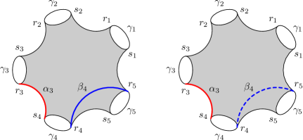
Figure 5.

This constructed surface has genus $g=n-1$ and admits the order $g+1$ rotation extended from the rotation on the $n$-holed spheres. Geometry of this closed surface is determined by the cuff length $c$ of the two $n$-holed spheres. We denote this surface by $S_{g}(c,0)$.

Now we begin to construct $S_{g}(c,t)$ for $t>0$. In $S_{g}(c,0)$, we denote a cuff of the $n$ holed sphere by $\gamma_{k}$ for $k=1,2,\dots,g+1$. We conduct a Fenchel-Nielsen deformation on $S(c,0)$ along all the $\gamma_{k}$ curves. The time and orientation of the deformation at every $\gamma_{k}$ is the same so that the resulting surface preserves the order $g+1$ otation on $S_{g}(c,0)$. We assume the time of the Fenchel-Nielsen deformation is $t$ and denote the resulting surface as $S_{g}(c,t)$.

There is a $c_{1}>0$ such that on the surface $S_{g}(c_{1},0)$, $l(\alpha_{k})=l(\gamma_{k})$. This surface is the surface $S^{1}_{g}$. The shortest geodesics of $S^{1}_{g}$ consist of $\alpha_{k}$ and $\gamma_{k}$ for $k=1,2,\dots,g+1$ by the proof of [APP11, Theorem 3].

In a surface $S_{g}(c,t)$, we let $\beta_{k}$ be the image of $\alpha_{k}$ by a Dehn twist along $\gamma_{k+1}$ (Figure 5). Orientation of this Dehn twist is required to be opposite to the Fenchel-Nielsen deformation so that length of $\beta_{k}$ decreases as $t$ increases when $t$ is closed to $0$.

There is a pair $(c_{2},t_{2})$ such that on the surface $S_{g}(c_{2},t_{2})$, $l(\alpha_{k})=l(\beta_{k})=l(\gamma_{k})$. This surface is the surface $S^{2}_{g}$. The shortest geodesics of $S^{2}_{g}$ consist of $\alpha_{k}$, $\beta_{k}$ and $\gamma_{k}$ for $k=1,2,\dots,g+1$ by [BGW19, Proposition 4].

7.2. Symmetry on $S(c,t)$

By the construction of the surface $S_{g}(c,t)$, for any $c>0$ and $0\leq t\leq c/2$, $S(c,t)$ admits an order $g+1$ rotation rotation, denoted $\sigma$ (Figure 6(a)). Besides this rotation, $S_{g}(c,t)$ admits an order $2$ rotation $\tau$ exchanging the two $n$-holed spheres (Figure 6(b)) and an order $2$ rotation $\varsigma$ extended from an order $2$ rotation on one of the $n$-holed spheres. We denote the symmetric group on $S(c,t)$ generated by $\sigma$, $\tau$ and $\varsigma$ by $G$.

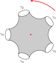
(a) The rotation $\sigma$.

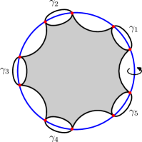
(b) The rotation $\tau$.

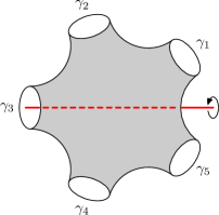
(c) The rotation $\varsigma$.

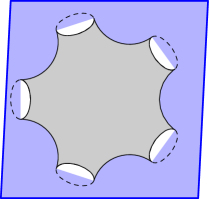
(d) The reflection $\rho$.

Figure 6.

On the surface $S_{g}(c,0)$, there is a reflection $\rho$ extended from the reflection on one of the $n$-holed spheres exchanging the two polygons of the $n$-holed sphere (Figure 6(d)). The symmetric group generated by $\sigma$, $\tau$, $\varsigma$ and $\rho$ is denoted by $\bar{G}$.

Remark 7.1.

For a reflection on the $n$-holed sphere, this reflection can be extended to the whole surface $S_{g}(c,t)$ only if $t=0$ or $t=c/2$.

The reflection on $S_{g}(c,c/2)$ (denoted by $\rho_{c/2}$) is not conjugate to $\rho$. This is because their fixed point sets are different. The fixed points of $\rho$ on $S_{g}(c,0)$ consist of $g+1$ curves (the $\beta_{k}$ curves), whille fixed points of $\rho_{c/2}$ consist of one curve (when $g$ is even) or two curves (when $g$ is odd), see Figure 7.

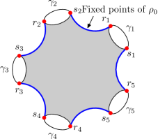
(a) The fixed point set of $\rho$ on $\Sigma_{g}(c,0)$.

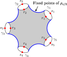
(b) The fixed point set of $\rho_{c/2}$ on $\Sigma_{g}(c,c/2)$.

Figure 7.

The surface $S_{g}^{1}$ has been proved to be a critical point of the systole function, see [FB19, Example 4.2, Proposition 6.3].

On the other hand, it is proved in [BGW19] that the surface $S_{g}^{2}$ is the surface with the maximal systole among the surfaces admitting the action of $G$. Then immediately by Proposition 6.5, $S_{g}^{2}$ is a critical point of the systole function.

Hence we have

Proposition 7.2.

The surfaces $S_{g}^{1}$ and $S_{g}^{2}$ are critical points of the systole function.

7.3. Distance

The aim of this subsection is to bound the Teichmüller distance between $S^{1}_{g}$ and $S^{2}_{g}$.

To get an upperbound of $d_{\mathcal{T}}(S^{1}_{g},S^{2}_{g})$, we need an intermediate surface. We assume the parameter $S^{1}_{g}=S_{g}(c_{1},0)$ and $S^{2}_{g}=S_{g}(c_{2},t_{2})$. Then the intermediate surface is the surface $S_{g}(c_{2},0)$. Distance between $S^{1}_{g}$ and $S^{2}_{g}$ is bounded from above by the sum of $d_{\mathcal{T}}(S_{g}^{1},S(c_{2},0))$ and $d_{\mathcal{T}}(S(c_{2},0),S_{g}^{2})$.

7.3.1. The distance between $S_{g}^{1}=S(c_{1},0)$ and $S(c_{2},0)$

We estimate this distance in three steps:

(1) Prove $\left\{S(c,0)|c>0\right\}$ is a Teichmüller geodesic induced by a Jenkins-Strebel differential on some surface $S(c,0)$.

(2) Calculate distance between two points on the Teichmüller geodesic. This distance is given by a ratio of extremal lengths of a curve on the two surfaces.

(3) Estimate this distance expressed in extremal lengths by hyperbolic lengths using Maskit’s Theorem (Theorem 2.19).

For $c>0$, on the surface $S(c,0)$, we consider the cuffs of the $n$-holed spheres in $S(c,0)$, namely $\left\{\gamma_{k}\right\}_{k=1}^{g+1}$ and assign to each $\gamma_{k}$ a positive number $b$. Then by Theorem 2.18, $\left\{(\gamma_{k},b)\right\}_{k=1}^{g+1}$ induces a quadratic differential $q$ on $S(c,0)$.

Lemma 7.3.

The quadratic differential $q\in QD(S_{g}(c,0))$ is invariant under the action of $\bar{G}$.

Proof.

For $g\in\bar{G}$, the quadratic form $g^{*}q$ is induced by the set $\left\{(g^{-1}(\gamma_{k}),b)\right\}_{k=1}^{g+1}$. By the action of $\bar{G}$ on $S_{g}(c,0)$, $\left\{(g^{-1}(\gamma_{k}),b)\right\}_{k=1}^{g+1}=\left\{(\gamma_{k},b)\right\}_{k=1}^{g+1}$. Therefore $g^{*}q=q$ and $q$ is invariant. ∎

We consider the Teichmüller geodesic induced by $(S(c,0),q)$.

Lemma 7.4.

We denote the Teichmüller geodesic induced by $(S(c,0),q)$ as $l$. Then the Teichmüller geodesic $l$ coincides with the curve $\left\{S_{g}(c,0)|c>0\right\}$.

Proof.

Since $q$ is $\bar{G}$-invariant by Lemma 7.3, For any surface $S^{\prime}\in l$ the Beltrami coefficient of the Teichmüller map $f:S(c,0)\to S^{\prime}$ is $t\frac{\bar{q}}{q}$ for some $t\in(0,1)$. Hence this Beltrami coefficient is $\bar{G}$-invariant. Then by Proposition 6.4 (1), $\bar{G}$ isometrically acts on $S^{\prime}$ by

$$f\circ g\circ f^{-1}:S^{\prime}\to S^{\prime}$$

for any $g\in\bar{G}$.

Consider the set of cuffs of the $n$-holed spheres on $S_{g}(c,0)$, denoted $\left\{\gamma_{k}\right\}_{k=1}^{g+1}$. Its image $\left\{f(\gamma_{k})\right\}_{k=1}^{g+1}$ in $S^{\prime}$ cuts $S^{\prime}$ into two $n$-holed spheres. Then $\bar{G}$ isometrically acts on these two $n$-holed spheres as $\bar{G}$ acts on the two $n$-holed spheres in $S(c,0)$ divided by $\left\{\gamma_{k}\right\}_{k=1}^{g+1}$. Then $S^{\prime}$ is a $S(c^{\prime},0)$ surface, where $c^{\prime}$ is the length of $f(\gamma_{k})$ on $S^{\prime}$.

Therefore the Teichmüller geodesic $l$ is contained in the curve $\left\{S_{g}(c,0)|c>0\right\}$. Then by the completeness of Teichmüller geodesics, $\left\{S_{g}(c,0)|c>0\right\}$ coincides with $l$. ∎

Distance between two points on a Teichmüller geodesic has been given by (2.5). Now we are ready to acomplish the third step.

Finally we have

Proposition 7.5.

For $S_{g}^{1}=S_{g}(c_{1},0)$ and $S_{g}{(c_{2},0)}$, we have

$$d_{\mathcal{T}}(\Sigma_{g}^{1},\Sigma_{g}^{1,2})\leq 0.65.$$

Proof.

Recall that $c_{1}$ and $c_{2}$ are the systole of $S_{g}^{1}$ and $S_{g}^{2}$ respectively. Then $c_{1}=4\operatorname{arcsinh}\sqrt{\cos\frac{\pi}{g+1}}$ by [APP11] and $c_{2}$is given by the formula in [BGW19, Theorem 1]. Then we use the following lemma to get the Teichmüller distance.

Lemma 7.6.

For hyperbolic surfaces $S_{g}(c_{1},0)$ and $S_{g}{(c_{2},0)}$ with $c_{1}<c_{2}$, the Teichmüller distance between these two surfaces is bounded from above by

$$\frac{1}{2}\log\frac{\pi c_{2}}{2\theta c_{1}},$$

where

$$\cos\theta=\left(1+\frac{\cos^{2}\frac{\pi}{g+1}}{\sinh^{2}\frac{c_{2}}{4}}\right)^{-\frac{1}{2}}$$

.

Proof.

For $i=1,2$, we let $\{\gamma_{k}^{(i)}\}_{k=1}^{g+1}$ be the cuffs in $S_{g}(c_{i},0)$, $q_{i}\in QD(S_{g}(c_{i},0))$ be the quadratic differential induced by $\{(\gamma_{k}^{(i)},b)\}_{k=1}^{g+1}$ for some $b>0$ and $R_{k}^{(i)}$ be the characteristic ring domain of $\gamma_{k}^{(i)}$. Then by Theorem 2.19

(7.1) $$\operatorname{Ext}_{\gamma_{k}^{(1)}}(R_{k}^{(1)})\geq\operatorname{Ext}_{\gamma_{k}^{(1)}}(S_{g}(c_{1},0))\geq\frac{l(\gamma_{k}^{(1)})}{\pi}=\frac{c_{1}}{\pi}.$$

The set of characteristic ring domains $\{R_{k}^{(2)}\}_{k=1}^{g+1}$ is invariant under the $\bar{G}$-action. Then by the symmetry of $\bar{G}$, in $S_{g}(c_{2},0)$, the ring domains $R_{k}^{(2)}$, $k=1,\dots,g+1$ are bounded by the hyperbolic geodesics, connecting a center of the $2n$-polygons and a middle point of the seams (Figure 9), otherwise $\{R_{k}^{(2)}\}_{k=1}^{g+1}$ is not $\bar{G}$-invariant.

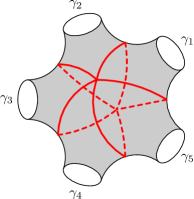
Figure 8. Charateristic ring domains

Figure 9. Calculate $s_{2}/2$

Therefore, if the seam length of $n$-holed spheres of $S_{g}(c_{2},0)$ is $s_{2}$, then the collar $C_{k}$ of $\gamma_{k}^{(2)}$ with width $s_{2}/s$ is contained in the characteristic ring domain $R_{k}^{(2)}$.

The seam length $s_{2}$ is given by the formula in trirectangle (2.7), see Figure 9

(7.2) $$\sinh\frac{s_{2}}{2}\sinh\frac{c_{2}}{4}=\cos\frac{\pi}{g+1}.$$

Therefore, by Theorem 2.19

(7.3) $$\operatorname{Ext}_{\gamma_{k}^{(2)}}(R_{k}^{(2)})\leq\operatorname{Ext}_{\gamma_{k}^{(2)}}(C_{k})\leq\frac{l(\gamma_{k}^{(2)})}{2\arccos\frac{1}{\cosh({s_{2}}/{2})}}=\frac{c_{2}}{2\arccos\frac{1}{\cosh({s_{2}}/{2})}}$$

By combining (2.5) (7.1) (7.3) and (7.2), this Lemma holds.

∎

Proposition 7.5 follows immediately by Lemma 7.6. ∎

7.3.2. The distance between $S_{g}(c_{2},0)$ and $S_{g}^{2}=S_{g}(c_{2},t_{2})$

Recall that $S_{g}(c_{2},t_{2})$ is obtained from $S_{g}(c_{2},0)$ by a Fenchel-Nielsen deformation along the cuffs $\left\{\gamma_{k}\right\}_{k=1}^{g+1}$ in $S(c_{2},0)$ with time $t_{2}$. If we can construct a homeomorphism $h:S_{g}(c_{2},0)\to S_{g}(c_{2},t_{2})$ such that for a collar $C_{k}$ of $\gamma_{k}$ where $k=1,2,\dots,g+1$, $h$ is an isometry outside all these collars, then Teichmüller distance between $S_{g}(c_{2},0)$ and $S_{g}(c_{2},t_{2})$ is bounded from above by the $\frac{1}{2}\log K(h)$ fo the dilatation $K(h)$ and $K(h)$ equals $K(h|_{C_{k}})$ the dilatation of $h$ restricted on some $C_{k}$.

Proposition 7.7.

For $\Sigma_{g}^{2}$ and $\Sigma_{g}^{1,2}$, we have

$$d_{\mathcal{T}}(\Sigma_{g}^{2},\Sigma_{g}^{1,2})\leq 1.6450.$$

Proof.

We prove this proposition by constructing the homeomorphism $h$ and calculate its dilatation on the largest colar of $\gamma_{k}$.

We let $C_{k}$ be the collar of $\gamma_{k}$ with the width $s_{2}/$, where $s_{2}$ is the seam length of the $n$-holed spheres as in Lemma 7.6. The homeomorphism $h$ on $C_{k}$ is described in the Figure 11. A geodesic $l$ orthogonal to the core curve $\gamma_{k}$ is always mapped to a geodesic $l^{\prime}$. The line $l$ is required to intersect $l^{\prime}$ at a point $p$ on $\gamma_{k}$. The projection of one of the end points of $l^{\prime}$ (denoted $p^{\prime}$) is required to has distance $t_{2}/2$ to $p$.

Figure 10. The homeomorphism $h|_{C_{k}}$.

Figure 11. The lift of ${C_{k}}$ to $\mathbb{H}^{2}$.

We let $h$ outside the collars be an isometry on this surface of $S_{g}(c_{2},0)$, then the homeomorphism $h$ maps $S_{g}(c_{2},0)$ to $S_{g}(c_{2},t_{2})$ by the construction on the collars.

The rest of the proof is on the calculation of $K(h)$ on the collar $C_{k}$. To calculate this dilatation, we lift $C_{k}$ on the upper half plane $\mathbb{H}^{2}$ (Figure 11).

We lift $\gamma_{k}$ to the $y$-axis, assuming $p=i$ and $p^{\prime}=ie^{t_{2}/2}$. The collar of $\gamma_{k}$ with width is lifted to a strip $\left\{re^{i\varphi}\in\mathbb{H}^{2}|-\theta+\pi/2<\varphi<\theta+\pi/2\right\}$, where

(7.4) $$\cos\theta=\frac{1}{\cosh\frac{s_{2}}{2}}.$$

In this strip, $l$ is the unit circle and $l^{\prime}$ is the geodesic connecting $i$ and $\exp(t_{2}/2+i\sin\theta)$.

The homeomorphism $h$ can be expressed in the form

$$h(re^{i\varphi})=r\Phi(\varphi)e^{i\varphi}.$$

When $r=1$, $h$ maps $l$ to $l^{\prime}$ in Figure 11. By this requirement we can calculate that

(7.5) $$\Phi(\varphi)=\sinh\left(\frac{t_{2}}{2}\right)\frac{\cos\varphi}{\sin\theta}+\sqrt{\sinh^{2}\left(\frac{t_{2}}{2}\right)\frac{\cos^{2}\varphi}{\sin^{2}\theta}+1}.$$

The dilatation $K(h)$ is given by

(7.6) $$K(h)=\frac{|h_{z}|+|h_{\bar{z}}|}{|h_{z}|-|h_{\bar{z}}|}=\frac{\sqrt{\Phi^{2}+\frac{1}{4}\Phi^{\prime 2}}+\frac{1}{2}|\Phi^{\prime}|}{\sqrt{\Phi^{2}+\frac{1}{4}\Phi^{\prime 2}}-\frac{1}{2}|\Phi^{\prime}|}.$$

Here $z=re^{i\varphi}$ and $\bar{z}=re^{-i\varphi}$.

Combining (7.6), (7.5) (7.4) (7.2) and the formula for $(c_{2},t_{2})$ in [BGW19, Theorem 1], we obtain the distance $d_{\mathcal{T}}(S_{g}(c_{2},0),S_{g}(c_{2},t_{2}))\leq\frac{1}{2}\log K(h)\leq 1.6450$ (see Figure 12).

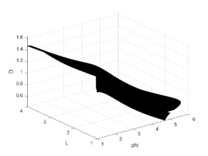
Figure 12. The dilation of $h$. Here $D$ is $K(h)$, $phi$ is the variable $\varphi$ and $L$ is $4\cos^{2}\frac{\pi}{g+1}$.

∎

Hence by Proposition 7.5 and 7.7, we have

Theorem 7.8.

For any $g\geq 2$,

$$d_{\mathcal{T}}(S_{g}^{1},S_{g}^{2})\leq 2.3.$$

8. Large distance

8.1. The $S_{g}^{3}$ surface

We take the $X(\Gamma)$ surface in [FBR20] when $n=2$ as the surface $S_{g}^{3}$. We briefly describe this surface for completeness.

We consider the $4$-holed sphere admitting the order $4$-rotation. We pick infinitely many copies of the $4$-holled sphere $\left\{P_{k}\right\}_{k=-\infty}^{+\infty}$ and glue them together into a surface $S_{\infty}$ with infinite genus as shown in Figure 13.

Figure 13. The surface $S_{\infty}$

The surface $S_{\infty}$ admits an isometric action $\psi:S_{\infty}\to S_{\infty}$, whic takes every $P_{k}$ to $P_{k+1}$. The surface $S^{3}_{g}$ is the quotient $S_{\infty}/\langle\psi^{g-1}\rangle$. When $g\geq 13$, $S_{g}^{3}$ is a local maximal point of the systole function.

8.2. The distance between $S_{g}^{1}$ and $S_{g}^{3}$

This istance is obtained from diameter comparison. Diameter of $S_{g}^{3}$ is comparable with $g$ while diameter of $S_{g}^{1}$ is comparable with $\log g$. Then distance between these two surfaces is comparable with $\log g$ by the method in the proof of [RT13, Lemma 5.1].

Proposition 8.1.

For the diameter of the surface $S_{g}^{3}$, we have

$$\operatorname{diam}(S_{g}^{3})\geq 0.6\left\lfloor\frac{g-5}{2}\right\rfloor.$$

Proof.

By the construction, the surface $S_{g}^{3}$ consists of $g-1$ four-holed spheres $P_{k}$, $k=1,2,\dots,g-1$.

When $g\geq 5$, for any $x\in P_{k}$ and $y\in P_{k+2}$ for some $k$, a curve connecting $x$ and $y$ must pass at least one of the four-holed spheres except $P_{k}$ and $P_{k+2}$. Without loss of generality, we assume this curve passes $P_{k+1}$, then this curve, if given an orientation, enters $P_{k+1}$ at one cuff and leaves $P_{k+1}$ at another cuff. Therefore, $d(x,y)$ is bounded from below by the distance between neighboring cuffs of $P_{k+1}$. We denote this distance by $d$. Then inductively, when $k\leq(g-1)/2$, distance between $x\in P_{1}$ and $y\in P_{k}$ is at least $d\lfloor\frac{g-1}{2}-2\rfloor$. Hence

$$\operatorname{diam}(S_{g}^{3})\geq\left\lfloor\frac{g-1}{2}-2\right\rfloor.$$

The rest of this proof is to calculate $d$. The distance $d$ is actually the seam length of the four-holed spheres. The seam length $d$ is determined by the cuff length (denoted $c$) of the four-holed sphere by (8.1). In Figure 15, one of the two octagons forming the four-holed sphere, we have

(8.1) $$\sinh|AB|\sinh|BC|=\cos\angle O\text{ namely }\sinh\frac{c}{4}\sinh\frac{d}{2}=\cos\frac{\pi}{4}.$$

According to [FBR20, Lemma 2.5], the cuff length of the four-holed spheres is approximately $6.980$. Then by (8.1), this proposition holds. ∎

Figure 14. The right-angled octagon

Figure 15. The polygon $Q$

For the surface $S_{g}^{1}$ we have

Proposition 8.2.

The diameter of the surface $S_{g}^{1}$ satisfies

$$\operatorname{diam}(S_{g}^{1})<4\log\left(\frac{4g+4}{\pi}\right).$$

Proof.

Recall that the surface $S_{g}^{1}$ consists of two $g+1$-holed spheres and each of the $g+1$-holed sphere consists of two right-angled regular ($2g+2$)-gons. For any $x,y\in S_{g}^{1}$, for the two (possibly coicide) regular ($2g+2$)-polygons containing $x$ and $y$, there is a curve connecting $x$ and $y$, contained in the union of these two polygons (see Figure 16). Therefore, if we denote one of the four regular $2g+2$ polygons by $Q$, then

Figure 16. The path between $x$ and $y$

$$\operatorname{diam}(S_{g}^{1})\leq 2\operatorname{diam}(Q),$$

The diameter of $Q$ is realized by $2|OB|$ in Figure 15. In the triangle $\triangle OAB$, by (2.6),

$$\cosh|OB|=\cot\angle O\cot\angle B$$

namely

$$\cosh|OB|=\cot\frac{\pi}{4}\cot\frac{\pi}{2g+2}=\cot\frac{\pi}{2g+2}<\frac{2g+2}{\pi}.$$

Therefore

$$\operatorname{diam}(S_{g}^{1})\leq 2\operatorname{diam}(Q)\leq 4|OB|\\ <4\operatorname{arccosh}\left(\frac{2g+2}{\pi}\right)<4\log\left(\frac{4g+4}{\pi}\right).$$

∎

Now we are ready to prove

Theorem 8.3.

When $g\geq 13$,

$$d_{\mathcal{T}}(S_{g}^{1},S_{g}^{3})>\frac{1}{2}\log(g-6)-\frac{1}{2}\log\left(\frac{40}{3}\log\left(\frac{4g+4}{\pi}\right)\right).$$

Proof.

The proof here is similar to the proof of [RT13, Lemma 5.1].

We let $f:S_{g}^{1}\to S_{g}^{3}$ be a Lipschitz homeomorphism with $L(f)=d_{L}(S_{g}^{1},S_{g}^{3})$ (The existence of this homeomorphism is verified in [Thu98]. ). By Proposition 8.1, we pick $x,y\in S_{g}^{3}$ with $d(x,y)\geq 0.6\left\lfloor\frac{g-5}{2}\right\rfloor$. By Proposition 8.2, $d(f^{-1}(x),f^{-1}(y))<4\log\left(\frac{4g+4}{\pi}\right)$. Then

$$L(f)\geq\frac{d(x,y)}{d(f^{-1}(x),f^{-1}(y))}>\frac{0.6\left\lfloor\frac{g-5}{2}\right\rfloor}{4\log\left(\frac{4g+4}{\pi}\right)}>\frac{3(g-6)}{40\log\left(\frac{4g+4}{\pi}\right)}.$$

Hence

$$d_{L}(S_{g}^{1},S_{g}^{3})=\log L(f)>\log(g-6)-\log\left(\frac{40}{3}\log\left(\frac{4g+4}{\pi}\right)\right).$$

By (2.1),

$$d_{\mathcal{T}}(S_{g}^{1},S_{g}^{3})\geq\frac{1}{2}d_{L}(\Sigma_{g}^{1},\Sigma_{g}^{3})>\frac{1}{2}\log(g-6)-\frac{1}{2}\log\left(\frac{40}{3}\log\left(\frac{4g+4}{\pi}\right)\right).$$

∎

References

- [Ahl06] Lars Valerian Ahlfors. Lectures on quasiconformal mappings, volume 38. American Mathematical Soc., 2006.
- [Akr03] Hugo Akrout. Singularités topologiques des systoles généralisées. Topology, 42(2):291–308, 2003.
- [APP11] James W Anderson, Hugo Parlier, and Alexandra Pettet. Small filling sets of curves on a surface. Topology and its Applications, 158(1):84–92, 2011.
- [APP16] James W Anderson, Hugo Parlier, and Alexandra Pettet. Relative shapes of thick subsets of moduli space. American Journal of Mathematics, 138(2):473–498, 2016.
- [BGW19] Sheng Bai, Yue Gao, and Jiajun Wang. Maximal systole of hyperbolic surface with largest extendable abelian symmetry. arXiv preprint arXiv:1911.10474, 2019.
- [Bus10] Peter Buser. Geometry and spectra of compact Riemann surfaces. Springer Science & Business Media, 2010.
- [FB19] Maxime Fortier Bourque. Hyperbolic surfaces with sublinearly many systoles that fill. Commentarii Mathematici Helvetici, 2019.
- [FBR20] Maxime Fortier Bourque and Kasra Rafi. Local maxima of the systole function. Journal of the European Mathematical Society, 2020.
- [FKM13] Alastair Fletcher, Jeremy Kahn, and Vladimir Markovic. The moduli space of riemann surfaces of large genus. Geometric and Functional Analysis, 23(3):867–887, 2013.
- [HZ86] John Harer and Don Zagier. The euler characteristic of the moduli space of curves. Inventiones mathematicae, 85(3):457–485, 1986.
- [IT12] Yoichi Imayoshi and Masahiko Taniguchi. An introduction to Teichmüller spaces. Springer Science & Business Media, 2012.
- [Ji14] Lizhen Ji. Well-rounded equivariant deformation retracts of teichmüller spaces. L’Enseignement Mathématique, 60(1):109–129, 2014.
- [Mas85] Bernard Maskit. Comparison of hyperbolic and extremal lengths. Ann. Acad. Sci. Fenn. Ser. AI Math, 10:381–386, 1985.
- [Mas09] Howard Masur. Geometry of teichmüller space with the teichmüller metric. Surveys in differential geometry, 14(1):295–314, 2009.
- [Mir07] Maryam Mirzakhani. Simple geodesics and weil-petersson volumes of moduli spaces of bordered riemann surfaces. Inventiones mathematicae, 167(1):179–222, 2007.
- [Mir13] Maryam Mirzakhani. Growth of weil-petersson volumes and random hyperbolic surface of large genus. Journal of Differential Geometry, 94(2):267–300, 2013.
- [MP19] Maryam Mirzakhani and Bram Petri. Lengths of closed geodesics on random surfaces of large genus. Commentarii Mathematici Helvetici, 94(4):869–889, 2019.
- [NWX20] Xin Nie, Yunhui Wu, and Yuhao Xue. Large genus asymptotics for lengths of separating closed geodesics on random surfaces. arXiv preprint arXiv:2009.07538, 2020.
- [RT13] Kasra Rafi and Jing Tao. The diameter of the thick part of moduli space and simultaneous whitehead moves. Duke Mathematical Journal, 162(10):1833–1876, 2013.
- [Sch99] Paul Schmutz Schaller. Systoles and topological morse functions for riemann surfaces. Journal of Differential Geometry, 52(3):407–452, 1999.
- [Str84] Kurt Strebel. Quadratic differentials. In Quadratic Differentials, pages 16–26. Springer, 1984.
- [Thu98] William P Thurston. Minimal stretch maps between hyperbolic surfaces. arXiv preprint math/9801039, 1998.
- [Wol87] Scott A Wolpert. Geodesic length functions and the nielsen problem. Journal of Differential Geometry, 25(2):275–296, 1987.
- [Wu19] Yunhui Wu. Growth of the weil–petersson inradius of moduli space. In Annales de l’Institut Fourier, volume 69, pages 1309–1346, 2019.
- [Wu20] Yunhui Wu. A new uniform lower bound on weil-petersson distance. arXiv preprint arXiv:2005.09196, 2020.