On the phase diagram of a three-dimensional dipolar model.

Abstract

The magnetic phase diagram at zero external field of an ensemble of dipoles with uniaxial anisotropy on a FCC lattice has been investigated from tempered Monte Carlo simulations. The uniaxial anisotropy is characterized by a random distribution of easy axes and its magnitude $\lambda_{u}$ is the driving force of disorder and consequently frustration. The phase diagram, separating the paramagnetic, ferromagnetic and spin-glass regions, was thus considered in the temperature, $\lambda_{u}$ plane. Here we interpret this phase diagram in terms of the more convenient variables namely the bare dipolar interaction and anisotropy energies $\epsilon_{d}$ and $\epsilon_{u}$ on the one hand and the volume fraction $\Phi$ on the other hand and compare the result with that corresponding to the random distribution of particles in the absence of anisotropy. We also display the nature of the ordered phase reached at low temperature by the ensemble of dipoles on the FCC lattice in terms of both the dipolar coupling and the texturation of the easy axes distribution when the latter is no more random. This system is aimed at modeling the magnetic phase diagram of supracrystals of magnetic nanoparticles.

In Ref.Russier et al. (2020) we investigated the phase diagram of an ensemble of dipolar hard spheres located on the nodes of a perfect FCC lattice. The phase diagram was investigated in the reduced temperature, disorder control parameter, ($T^{*},\lambda_{u}$) plane. Given the $1/r^{3}$ dependence of the dipole-dipole interaction (DDI), it has been found convenient to define the reduced temperature, $T^{*}=T/T_{r}$ through the reference temperature $T_{r}=(\Phi/\Phi_{m})(\epsilon_{d}/k_{B})$ where $\Phi$, $\Phi_{m}$ and $\epsilon_{d}$ are the volume fraction, its maximum value of the FCC lattice and the dipole-dipole energy for particles at contact. The disorder control parameter is nothing but the anisotropy energy (MAE) over DDI ratio, namely $\lambda_{u}=(\epsilon_{u}/\epsilon_{d})(\Phi_{m}/\Phi)$. Then the ($T^{*},\lambda_{u}$) phase diagram, displayed on figure (1), is qualitatively similar to those corresponding to the $\pm{}J$ Ising model Hasenbusch et al. (2007); Papakonstantinou and Malakis (2013). The essential feature is the succession at low temperature of long range order FM, quasi long range FM (QLRO-FM) plus transverse SG and SG phases with increasing values of $\lambda_{u}$. Now, when considering the system as a model for the magnetic phase diagram of supracrystals of bare magnetic nanoparticles characterized by given values of $\epsilon_{d}$ and $\epsilon_{u}$ where the volume fraction $\phi$ can be tuned through the thickness of the coating layer, it is convenient to translate the phase diagram in terms of $(k_{B}T/\epsilon_{u})$ and $(\Phi/\Phi_{m})(\epsilon_{d}/\epsilon_{u})$, the latter being understood as the increasing dipolar coupling through the increase of concentration at constant $\epsilon_{d}$ and $\epsilon_{u}$. This is shown on figure (2). In this represention, the dipolar lattice phase diagram appears qualitatively similar to the one deduced from experiments on the DMIM samples Petracic (2010). Furthermore one must limit the reachable part of this phase diagram to the region defined by $\Phi/\Phi_{m}\leq{}1$. Doing this we see, as diplayed on figure (3), that according to the value of ($\epsilon_{d}/\epsilon_{u}$), namely the relative importance of the dipolar coupling to the anisotropy energy, the FM-QLRO an the FM phases may be not reachable. In the limit $\epsilon_{d}/\epsilon_{u}\rightarrow\infty$, one gets only the PM/FM transition of the pure dipolar system on the FCC lattice free of anisotropy ($\epsilon_{u}=0$) Bouchaud and Zerah (1993); Russier and Ngo (2017); Russier et al. (2020) and all the non trivial features of the phase diagram are shrinked on the $\Phi=0$ line. Moreover, the ($(k_{B}T/\epsilon_{u}),(\Phi/\Phi_{m})(\epsilon_{d}/\epsilon_{u})$) phase diagram for particles located on the perfect FCC lattice can be directly compared to the one we have got Alonso et al. (2020) for the system of dipolar spheres frozen in a random hard sphere like distribution, in the absence of anisotropy, where the increasing disorder is quantified by $1-(\phi/\phi_{RPC})$, the volume fraction being then limited to the so-called RCP value, $\Phi_{RCP}\simeq{}0.64$, given on figure (4). It is also qualitively close to the one of dipolar Ising model on the SC lattice in terms of dilution Alonso and Fernández (2010), where however the ordered phase is anti-FM due to the lattice symmetry. Finally, we present on figure (5) the nature of the ordered phase at low temperature in terms of the dipolar coupling and the texturation of the easy axes distribution as was studied in Alonso et al. (2019); Russier and Alonso (2020) in the limit of infinitely strong anisotropy energy leading to the dipolar Ising model. As is the case above, the condition $\Phi/\Phi_{m}\leq{1}$ restricts the diagram to the left hand part defined by the abcissa $\leq(\epsilon_{d}/\epsilon_{u})$ and has been displayed for two particular cases corresponding to a weak and a strong dipolar coupling respectively.

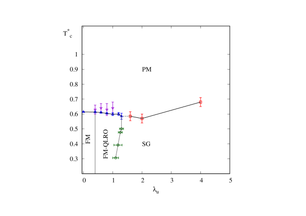
Figure 1: ($T_{c}/T_{r},\lambda_{u}$) phase diagram of the dipolar plus uniaxial anisotropy with random distribution of easy axes on a FCC lattice. $\lambda_{u}$ is the natural disorder control parameter.

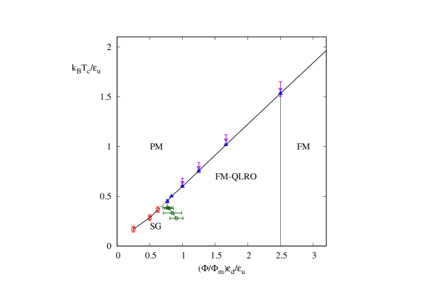
Figure 2: Phase diagram of figure (1), shown as $T_{c}$ in terms of increasing dipolar coupling for $\epsilon_{d}$ and $\epsilon_{u}$ considered as constant.

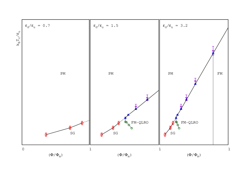
Figure 3: Same as figure (2) where the constraint $\Phi/\Phi_{m}\leq{1}$ is explicited for three characterisitc values of $\epsilon_{d}/\epsilon_{u}$ as indicated.

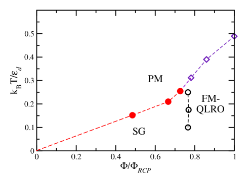
Figure 4: Phase diagram of the dipolar hard spheres distributed according to a frozen hard-sphere like distribution with $\epsilon_{u}=0$. The limiting value of the volumefraction, $\Phi_{RCP}$ is indicated.

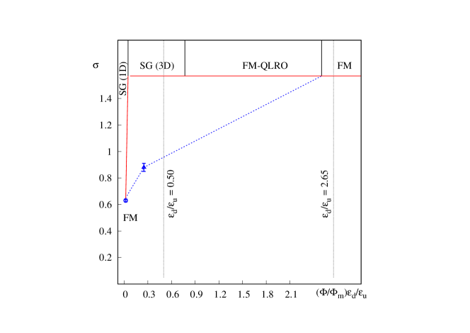
Figure 5: Nature of the ordered phase at low temperature for the FCC lattice in terms of the texturation quantified by the variance $\sigma$ of the easy axes distribution (see Ref. Alonso et al. (2019); Russier and Alonso (2020)) and the dipolar coupling $(\Phi/\Phi_{m})\epsilon_{d}/\epsilon_{u}$. Open circle and open triangle are the FM/SG transition in the dipolar Ising limit Russier and Alonso (2020), and $(\Phi/\Phi_{m})\epsilon_{d}/\epsilon_{u}=0.25$ Russier (2020) respectively. The dotted line is only indicative. The upper horizontal red line, $\sigma=\pi/2$ indicates the lower bound of random distribution of easy axes. The SG region is separated in the true dipolar SG (3D) and the limiting dipolar Ising SG (1D) obtained for $\lambda_{u}>30$ Russier et al. (2020). The reachable region is located on the left hand side of the line $(\Phi/\Phi_{m})\epsilon_{d}/\epsilon_{u}=\epsilon_{d}/\epsilon_{u}$ which is shown for a weak and a strong dipolar couplings as particular cases.

References

- Russier et al. (2020) V. Russier, J. J. Alonso, I. Lisiecki, A. T. Ngo, C. Salzemann, S. Nakamae, and C. Raepsaet, Phys. Rev. B 102, 174410 (2020).
- Hasenbusch et al. (2007) M. Hasenbusch, F. P. Toldin, A. Pelissetto, and E. Vicari, Phys. Rev. B 76, 184202 (2007).
- Papakonstantinou and Malakis (2013) T. Papakonstantinou and A. Malakis, Phys. Rev. E 87, 012132 (2013).
- Petracic (2010) O. Petracic, Superlattices and Microstructures 47, 569 (2010).
- Bouchaud and Zerah (1993) J. P. Bouchaud and P. G. Zerah, Phys. Rev. B 47, 9095 (1993).
- Russier and Ngo (2017) V. Russier and E. Ngo, Condensed Matter Physics 20, 33703 (2017).
- Alonso et al. (2020) J. J. Alonso, B. Allés, and V. Russier, Phys. Rev. B 102, 184423 (2020).
- Alonso and Fernández (2010) J.-J. Alonso and J.-F. Fernández, Phys. Rev. B 81, 064408 (2010).
- Alonso et al. (2019) J.-J. Alonso, B. Allés, and V. Russier, Phys. Rev. B 100, 134409 (2019), arXiv:1909.13573.
- Russier and Alonso (2020) V. Russier and J. J. Alonso, J. Phys.-Cond. Matt. 32, 135804 (2020).
- Russier (2020) V. Russier, (2020), unpublished.