General one-loop formulas for $H\rightarrow f\bar{f}\gamma$ and its applications

Abstract

We present general one-loop contributions to the decay processes $H\rightarrow f\bar{f}\gamma$ including all possible the exchange of the additional heavy vector gauge bosons, heavy fermions, and charged (also neutral) scalar particles in the loop diagrams. As a result, the analytic results are valid in a wide class of beyond the standard models. Analytic formulas for the form factors are expressed in terms of Passarino-Veltman functions in the standard notations of LoopTools. Hence, the decay rates can be computed numerically by using this package. The computations are then applied to the cases of the standard model, $U(1)_{B-L}$ extension of the standard model as well as two Higgs doublet model. Phenomenological results of the decay processes for all the above models are studied. We observe that the effects of new physics are sizable contributions and these can be probed at future colliders.

1 Introduction

After discovering the standard model-like (SM-like) Higgs boson [1, 2], one of the main purposes at future colliders like the high luminosity large hadron collider (HL-LHC) [3, 4] as well as future lepton colliders [5] is to probe the properties of this boson (mass, couplings, spin and parity, etc). In the experimental programs, the Higgs productions and its decay rates should be measured as precise as possible. Based on the measurements, we can verify the nature of the Higgs sector. In other words we can understand deeply the dynamic of the electroweak symmetry breaking. It is well-known that the Higgs sector is selected as the simplest case in the standard model (SM) which there is only a scalar doublet field. From theoretical viewpoints, there are no reasons for this simplest choice. Many of beyond the standard models (BSMs) have extended the Higgs sector (some of them have also expanded gauge sectors, introduced mass terms of neutrinos, etc). In these models many new particles are proposed, for examples, new heavy gauge bosons, charged and neutral scalar Higgs as well as new heavy fermions. These new particles may also contribute to the productions and decay of Higgs boson. It means that the more precise data and new theoretical approaches on the Higgs productions and its decay rates could provide us a crucial tool to answer the nature of the Higgs sector and, more important, to extract the new physics contributions.

Among all the Higgs decay channels, the processes $H\rightarrow f\bar{f}\gamma$ are great of interest at the colliders by following reasons. Firstly, the decay channels can be measured at the large hadron collider [6, 7, 8, 9]. Therefore, the processes can be used to test the SM at the high energy regions. Secondly, many of new particles as mentioned in the beginning of this section may propagate in the loop diagrams of the decay processes. Subsequently, the decay rates could provide a useful tool for constraining new physic parameters. Last but not least, apart from the SM-like Higgs boson, new neutral Higgs bosons in BSMs may be mixed with the SM-like one. These effects can be also observed directly by measuring of the decay rates of $H\rightarrow f\bar{f}\gamma$. As above reasons, the detailed theoretical evaluations for one-loop contributions to the decay of Higgs to fermion pairs and a photon within the SM and its extensions are necessary.

Theoretical implications for the decay $H\rightarrow f\bar{f}\gamma$ in the SM at the LHC have studied in Refs. [10, 11, 12]. Moreover, there have been many available computations for one-loop contributing to the decay processes $H\rightarrow f\bar{f}\gamma$ within the SM framework [13, 14, 15, 16, 17, 18, 19, 20]. The same evaluations for the Higgs productions at $e\gamma$ colliders have proposed in [21, 22]. While one-loop corrections to $H\rightarrow f\bar{f}\gamma$ in the context of the minimal super-symmetric standard model Higgs sector have computed in [23]. Furthermore, one-loop contributions for CP-odd Higgs boson productions in $e\gamma$ collisions have carried out in [24]. In this article, we present general formulas for one-loop contributing to the decay processes $H\rightarrow f\bar{f}\gamma$. The analytic results presented in the current paper are not only valid in the SM but also in many of BSMs in which new particles are proposed such as heavy vector bosons, heavy fermions, and charged (neutral) scalar particles that may propagate in the loop diagrams of the decay processes. The analytic formulas for the form factors are expressed in terms of Passarino-Veltman (PV) functions in standard notations of LoopTools [46]. As a result, they can be evaluated numerically by using this package. The calculations are then applied to the SM and many of beyond the SM such as the $U(1)_{B-L}$ extension of the SM [25], two Higgs doublet models (THDM) [27]. Phenomenological results of the decay processes for these models are also studied.

We also stress that our analytical results in the present paper can be also applied for many of BSMs framework. In particular, in the super-symmetry models, many super-partners of fermions and gauge bosons are introduced. Furthermore, with extending the Higgs sector, we encounter charged and neutral Higgs bosons in this framework. There are exist the extra charged gauge bosons in many electroweak gauge extensions, for examples, the left-right models (LR) constructed from the $SU(2)_{L}\times SU(2)_{R}\times U(1)_{Y}$ [28, 29, 30], the 3-3-1 models ($SU(3)_{L}\times U(1)_{X}$) [31, 32, 33, 34, 35, 36, 37], the $3$-$4$-$1$ models ($SU(4)_{L}\times U(1)_{X}$) [37, 38, 39, 40, 41, 42], etc. Analytic results in this paper already include the contributions these mentioned particles which may also exchange in the loop diagrams of the aforementioned decay processes. Phenomenological results for the decay processes in the above models are great of interest in future. These topic will be devoted in our future publications.

The layout of the paper is as follows: We first write down the general Lagrangian and introduce the notation for the calculations in the section $2$. We then present the detailed calculations for one-loop contributions to $H\rightarrow f\bar{f}\gamma$ in section $3$. The applications of this work to the SM, $U(1)_{B-L}$ extensions of the SM and THDM are also studied in this section. Phenomenological results for these models are analysed at the end of section $3$. Conclusions and outlook are devoted in the section $4$. In appendices, the checks for the computations are shown. We then review briefly $U(1)_{B-L}$ extensions of the SM and THDM in the appendices. Finally, Feynman rules and all involving couplings in the decay processes are shown.

2 Lagrangian and notations

In order to write down the general form of Lagrangian for a wide class of the BSMs, we start from the well-known contributions appear in the SM. We then consider the extra forms that extended from the SM. For example, the two Higgs doublet model [27] adding a new Higgs doublet that predict new charged and neutral scalar Higgs bosons; a model with a gauge symmetry $U(1)_{B-L}$ which proposes a neutral gauge boson $Z^{\prime}$ [25, 26], neutral Higgs; a minimal left-right models with a new non-Abelian gauge symmetry for electroweak interactions $SU(2)_{L}\times SU(2)_{R}\times U(1)_{B-L}$ [28, 29, 30] introducing many new particles including charged gauge bosons, neutral gauge bosons and charged Higgs bosons. The mentioned particles give one-loop contributions to the decays under consideration.

In this section, Feynman rules for the decay channels $H\rightarrow f\bar{f}\gamma$ are derived for the most general extension of the SM with considering all possible contributions from the mentioned particles. In this computation, we denote $V_{i},V_{j}$ for extra charged gauge bosons, $V_{k}^{0}$ for neutral gauge bosons. Moreover, $S_{i},S_{j}\;(S_{k}^{0})$ are charged (neutral) Higgs bosons respectively and $f_{i},f_{j}$ show for fermions. In general, the classical Lagrangian contains the following parts:

$$\mathcal{L}=\mathcal{L}_{f}+\mathcal{L}_{G}+\mathcal{L}_{\Phi}+\mathcal{L}_{Y}.$$ (1)

Where the fermion sector is given

$$\mathcal{L}_{f}=\bar{\psi}_{f}i\not{D}\psi_{f}$$ (2)

with $D_{\mu}=\partial_{\mu}-igT^{a}V_{\mu}^{a}+\cdots$. In this formula, $T^{a}$ is generator of the corresponding gauge symmetry. The gauge sector reads

$$\mathcal{L}_{G}=-\frac{1}{4}\sum\limits_{a}V^{a}_{\mu\nu}V^{a,\mu\nu}+\cdots$$ (3)

where $V^{a}_{\mu\nu}=\partial_{\mu}V^{a}_{\nu}-\partial_{\nu}V^{a}_{\mu}+gf^{abc}V^{b}_{\mu}V^{c}_{\mu}$ with $f^{abc}$ is structure constant of the corresponding gauge group. The scalar sector is expressed as follows:

$$\mathcal{L}_{\Phi}=\sum\limits_{\Phi}Tr[\left(D_{\mu}\Phi\right)^{{\dagger}}\left(D^{\mu}\Phi\right)]-V(\Phi).$$ (4)

We then derive all the couplings from the full Lagrangian. The couplings are parameterized in general forms and presented by following:

• By expanding the fermion sector, we can derive the vertices of vector boson $V$ with fermions. In detail, the interaction terms are parameterized as

  $$\mathcal{L}_{Vff}=\sum\limits_{f_{i},f_{j},V}\bar{f}_{i}\gamma^{\mu}(g_{Vff}^{L}P_{L}+g_{Vff}^{R}P_{R})f_{j}V_{\mu}+\cdots$$ (5)

  with $P_{L,R}=(1\mp\gamma_{5})/2$.

• Trilinear gauge and quartic gauge couplings are expanded from the gauge sector:

  $$\mathcal{L}_{VVV,VVVV} = \sum\limits_{V_{k}^{0},V_{i},V_{j}}g_{V_{k}^{0}V_{i}V_{j}}\Big{[}\partial_{\mu}V^{0}_{k,\nu}V_{i}^{\mu}V_{j}^{\nu}+V_{k,\nu}^{0}V_{i}^{\mu}\partial^{\nu}V_{j,\mu}+\cdots\Big{]}$$ (6)

  $$+\sum\limits_{V_{k}^{0},V_{l}^{0},V_{i},V_{j}}g_{V_{k}^{0}V_{l}^{0}V_{i}V_{j}}\Big{[}V^{0}_{k,\mu}V_{l,\nu}^{0}V_{i}^{\mu}V_{j}^{\nu}+\cdots\Big{]}+\cdots$$

• Next, the couplings of scalar $S$ to fermions are taken from the Yukawa part $\mathcal{L}_{Y}$. The interaction terms are expressed as follows:

  $$\mathcal{L}_{Sf_{i}f_{j}}=\sum\limits_{f_{i},f_{j},S}\bar{f}_{i}(g_{Sff}^{L}P_{L}+g_{Sff}^{R}P_{R})f_{j}S+\cdots$$ (7)

• The couplings of scalar $S$ to vector boson $V$ can be derived from the kinematic term of the Higgs sector. In detail, we have the interaction terms

  $$\mathcal{L}_{SVV,SSV,SSVV} = \sum\limits_{S,V_{i},V_{j}}g_{SV_{i}V_{j}}SV_{i}^{\mu}V_{j,\mu}+\sum\limits_{S_{i},S_{j},V}g_{S_{i}S_{j}V}[(\partial_{\mu}S_{i})S_{j}-(\partial_{\mu}S_{j})S_{i}]V^{\mu}$$ (8)

  $$+\sum\limits_{S_{i},S_{j},V_{k},V_{l}}g_{S_{i}S_{j}V_{k}V_{l}}S_{i}S_{j}V_{k}^{\mu}V_{l,\mu}+\cdots$$

• Finally, the trilinear scalar and quartic scalar interactions are from the Higgs potential $V(\Phi)$. The interaction terms are written as

  $$\mathcal{L}_{SSS,SSSS} = \sum\limits_{S_{i},S_{j},S_{k}}g_{S_{i}S_{j}S_{k}}S_{i}S_{j}S_{k}+\sum\limits_{S_{i},S_{j},S_{k},S_{l}}g_{S_{i}S_{j}S_{k},S_{l}}S_{i}S_{j}S_{k}S_{l}+\cdots$$ (9)

All of the Feynman rules corresponding to the above couplings giving one-loop contributions to the SM-like Higgs decays $H\to f\bar{f}\gamma$ are collected in appendix $D$. In detail, the propagators involving the decay processes in the unitary gauge are shown in Table 6. All the related couplings involving the decay channels are parameterized in general forms which are presented in Table 7 (we refer appendices $B$ and $C$ for two typical models).

3 Calculations

In this section, one-loop contributions to the decay processes $H\rightarrow f(q_{1})\bar{f}(q_{2})\gamma(q_{3})$ are calculated in detail. In the present paper, we consider the computations in the limit of $m_{f}\rightarrow 0$. All Feynman diagrams involving these processes can be grouped in to the following classes (seen Fig. 1).

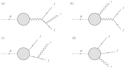
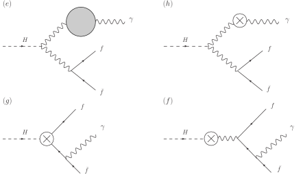
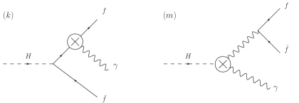
Figure 1: Types of Feynman diagrams involving to the SM-like Higgs decays $H\to f\bar{f}\gamma$

For on-shell photon, we confirm that the contributions of diagrams $(e+h)$ will be vanished. One can neglect the Yukawa coupling $y_{f}$ (since $m_{f}\rightarrow 0$) in this computation. As a result, the contributions of diagrams $(g+k+m)$ can be omitted. Furthermore, the diagrams $(a+f)$ are not contributed to the amplitude. Hence, we only have the contributions of $(b+c+d)$ which are separated into two kinds of the contributions. The first one is to the topology $b$ which is called $V_{k}^{0*}$ pole contributions. The second type (diagrams $c$ and $d$) belongs to the non-$V_{k}^{0*}$ pole contributions. We remind that $V_{k}^{0*}$ can include both $Z,\gamma$ in the SM and the arbitrary neutral vector boson $Z^{\prime}$ in many of the BSMs. General one-loop amplitude which obeys the invariant Lorentz structure can be decomposed as follows [20]:

$$\mathcal{A}_{\text{loop}} = \sum\limits_{k=1}^{2}\Big{\{}[q_{3}^{\mu}q_{k}^{\nu}-g^{\mu\nu}q_{3}\cdot q_{k}]\bar{u}(q_{1})(F_{k,R}\gamma_{\mu}P_{R}+F_{k,L}\gamma_{\mu}P_{L})v(q_{2})\Big{\}}\varepsilon^{*}_{\nu}(q_{3}).$$ (10)

In this equation, all form factors are computed as follows:

$$F_{k,L/R} = F_{k,L/R}^{\text{$V_{k}^{0*}$-poles}}+F_{k,L/R}^{\text{Non-$V_{k}^{0*}$}}$$ (11)

for $k=1,2$. Kinematic invariant variables involved in the decay processes are included: $q^{2}=q_{12}=(q_{1}+q_{2})^{2}$, $q_{13}=(q_{1}+q_{3})^{2}$ and $q_{23}=(q_{2}+q_{3})^{2}$.

We first write down all Feynman amplitudes for the above diagrams. With the help of Package-X [43], all Dirac traces and Lorentz contractions in $d$ dimensions are handled. Subsequently, the amplitudes are then written in terms of tensor one-loop integrals. By following tensor reduction for one-loop integrals in [44] (the relevant tensor reduction formulas are shown in appendix $A$), all tensor one-loop integrals are expressed in terms of PV-functions.

3.1 $V_{k}^{0*}$ pole contributions

In this subsection, we first arrive at the $V_{k}^{0*}$ pole contributions which are corresponding to the diagram $b$. In this group of Feynman diagrams, it is easily to confirm that the form factors follow the below relation:

$$F_{k,L/R}^{\text{$V_{k}^{0*}$-poles}}=F_{1,L/R}^{\text{$V_{k}^{0*}$-poles}}=F_{2,L/R}^{\text{$V_{k}^{0*}$-poles}}$$ (12)

Their analytic results are will be shown in the following subsections. All possible particles exchanging in the loop diagrams are included. We emphasize that analytic expressions for the form factors presented in this subsection cover the results in Ref. [45]. It means that we can reduce to the results for $H\to\nu_{l}\bar{\nu}_{l}\gamma$ of Ref. [45] by setting $f$ to $\nu_{l}$ and replacing the corresponding couplings. Furthermore, all analytic formulas shown in the following subsection cover all cases of $V_{k}^{0*}$ poles. For instance, when $V_{k}^{0*}\rightarrow\gamma^{*}$, we then set $M_{V^{0}_{k}}=0$, $\Gamma_{V^{0}_{k}}=0$. In addition, $V_{k}^{0*}$ becomes $Z$ (or $Z^{\prime}$) boson, we should fix $M_{V^{0}_{k}}=M_{Z}$ and $\Gamma_{V^{0}_{k}}=\Gamma_{Z}$ (or $Z^{\prime}$) respectively.

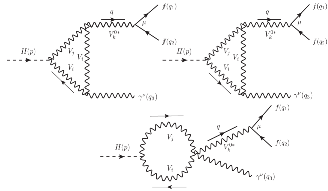
Figure 2: One-loop triangle diagrams with exchanging vector boson $V_{i,j}$ particles in the loop.

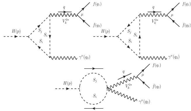
Figure 3: One-loop triangle diagrams with exchanging scalar boson $S_{i,j}$ particles in loop.

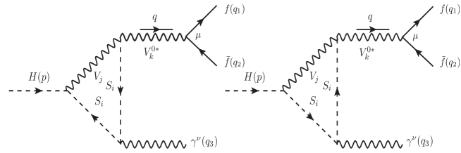
Figure 4: One-loop triangle diagrams with exchanging two scalar bosons $S_{i}$ and a vector boson $V_{j}$ particles in the loop.

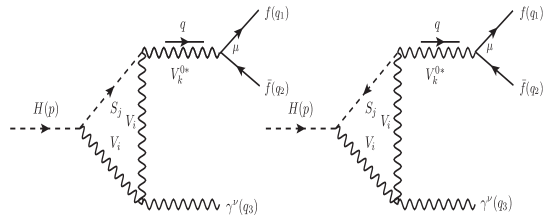
Figure 5: One-loop triangle diagrams with exchanging a scalar boson $S_{j}$ and two vector bosons $V_{i}$ in the loop.

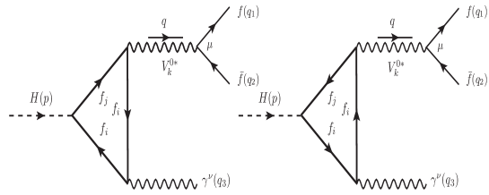
Figure 6: One-loop triangle diagrams with exchanging charged fermion $f_{i,j}$ particles in loop.

We begin with one-loop triangle Feynman diagrams which all vector bosons $V_{i,j}$ are in the loop (seen Fig. 2). One-loop form factors of this group of Feynman diagrams are expressed in terms of the PV functions as follows:

$$F_{k,L}^{\text{$V_{k}^{0*}$-poles}}|_{V_{i},V_{j}} = \dfrac{eQ_{V}}{16\pi^{2}}\sum\limits_{V_{i},V_{j},V^{0}_{k}}\dfrac{g_{HViVj}\;g_{V^{0}_{k}ff}^{L}}{M_{V_{i}}^{2}M_{V_{j}}^{2}(q^{2}-M_{V^{0}_{k}}^{2}+i\Gamma_{V^{0}_{k}}M_{V^{0}_{k}})}\times$$

$$\times\Bigg{\{}\Big{[}2g_{V^{0}_{k}AV_{i}V_{j}}(M_{H}^{2}-M_{V_{j}}^{2})+g_{V^{0}_{k}V_{i}V_{j}}(M_{H}^{2}+M_{V_{i}}^{2}+M_{V_{j}}^{2})\Big{]}B_{11}(M_{H}^{2},M_{V_{i}}^{2},M_{V_{j}}^{2})$$

$$+\Big{[}g_{V^{0}_{k}V_{i}V_{j}}(M_{H}^{2}+3M_{V_{i}}^{2}-M_{V_{j}}^{2})-2g_{V^{0}_{k}AV_{i}V_{j}}M_{V_{i}}^{2}\Big{]}B_{1}(M_{H}^{2},M_{V_{i}}^{2},M_{V_{j}}^{2})$$

$$+2M_{V_{i}}^{2}(g_{V^{0}_{k}V_{i}V_{j}}-g_{V^{0}_{k}AV_{i}V_{j}})B_{0}(M_{H}^{2},M_{V_{i}}^{2},M_{V_{j}}^{2})$$

$$+2g_{V^{0}_{k}AV_{i}V_{j}}\Big{[}M_{H}^{2}B_{111}+B_{00}+2B_{001}\Big{]}(M_{H}^{2},M_{V_{i}}^{2},M_{V_{j}}^{2})$$

$$+4g_{V^{0}_{k}V_{i}V_{j}}M_{V_{i}}^{2}\Big{(}M_{V_{i}}^{2}+3M_{V_{j}}^{2}-q^{2}\Big{)}C_{0}(0,q^{2},M_{H}^{2},M_{V_{i}}^{2},M_{V_{i}}^{2},M_{V_{j}}^{2})$$

$$+2g_{V^{0}_{k}V_{i}V_{j}}\Big{[}M_{H}^{2}(M_{V_{i}}^{2}+M_{V_{j}}^{2}-q^{2})+M_{V_{i}}^{4}+M_{V_{j}}^{4}+(4d-6)M_{V_{i}}^{2}M_{V_{j}}^{2}$$

$$\hskip 56.9055pt-q^{2}(M_{V_{i}}^{2}+M_{V_{j}}^{2})\Big{]}(C_{22}+C_{12})(0,q^{2},M_{H}^{2},M_{V_{i}}^{2},M_{V_{i}}^{2},M_{V_{j}}^{2})$$

$$+2g_{V^{0}_{k}V_{i}V_{j}}\Big{[}M_{H}^{2}(M_{V_{i}}^{2}+M_{V_{j}}^{2}-q^{2})+3M_{V_{i}}^{4}-M_{V_{j}}^{4}+(4d-6)M_{V_{i}}^{2}M_{V_{j}}^{2}$$

$$\hskip 85.35826pt-q^{2}(3M_{V_{i}}^{2}-M_{V_{j}}^{2})\Big{]}C_{2}(0,q^{2},M_{H}^{2},M_{V_{i}}^{2},M_{V_{i}}^{2},M_{V_{j}}^{2})\Bigg{\}},$$

$$F_{k,R}^{\text{$V_{k}^{0*}$-poles}}|_{V_{i},V_{j}} = F_{k,L}^{\text{$V_{k}^{0*}$-poles}}|_{V_{i},V_{j}}\Big{(}g_{V^{0}_{k}ff}^{L}\rightarrow g_{V^{0}_{k}ff}^{R}\Big{)}.$$ (14)

The results are written in terms of $B$- and $C$-functions. We note that one-loop amplitude for each diagram in Fig. 2 may decompose into tensor one-loop up to rank $R=6$. However, after taking into account all diagrams, the amplitude for this subset Feynman diagrams is only expressed in terms of the tensor integrals up to rank $R=2$. As a result, we have up to $C_{22}$-functions contributing to the form factors. Furthermore, some of them may contain UV divergent but after summing all these functions, the final results are finite. The topic will be discussed at the end of this section.

We next concern one-loop triangle Feynman diagrams with $S_{i},\;S_{j}$ in the loop (as described in Fig. 3). The corresponding one-loop form factors are given:

$$F_{k,L}^{\text{$V_{k}^{0*}$-poles}}|_{S_{i},S_{j}} = \dfrac{eQ_{S}}{4\pi^{2}}\sum\limits_{S_{i},S_{j},V^{0}_{k}}\dfrac{g_{HS_{i}S_{j}}\,g_{V^{0}_{k}S_{i}S_{j}}\,g_{V^{0}_{k}ff}^{L}}{M_{H}^{2}q^{2}(M_{H}^{2}-q^{2})(q^{2}-M_{V^{0}_{k}}^{2}+i\Gamma_{V^{0}_{k}}M_{V^{0}_{k}})}\times$$

$$\times\Bigg{\{}(q^{2}-M_{H}^{2})\Big{[}A_{0}(M_{S_{i}}^{2})-A_{0}(M_{S_{j}}^{2})\Big{]}$$

$$\hskip 14.22636pt+M_{H}^{2}(M_{S_{i}}^{2}-M_{S_{j}}^{2}-q^{2})B_{0}(q^{2},M_{S_{i}}^{2},M_{S_{j}}^{2})$$

$$\hskip 14.22636pt+q^{2}(M_{H}^{2}-M_{S_{i}}^{2}+M_{S_{j}}^{2})B_{0}(M_{H}^{2},M_{S_{i}}^{2},M_{S_{j}}^{2})$$

$$\hskip 14.22636pt+2M_{H}^{2}q^{2}(M_{H}^{2}-q^{2})C_{12}(0,q^{2},M_{H}^{2},M_{S_{i}}^{2},M_{S_{i}}^{2},M_{S_{j}}^{2})\Bigg{\}},$$

$$F_{k,R}^{\text{$V_{k}^{0*}$-poles}}|_{S_{i},S_{j}} = F_{k,L}^{\text{$V_{k}^{0*}$-poles}}|_{S_{i},S_{j}}\Big{(}g_{V^{0}_{k}ff}^{L}\rightarrow g_{V^{0}_{k}ff}^{R}\Big{)}.$$ (16)

Similarly, we have the contributions of one-loop triangle Feynman diagrams with exchanging scalar boson $S_{i}$ and vector boson $V_{j}$ in the loop. The Feynman diagrams are depicted as in Fig. 4. Applying the same procedure, one has the form factors

$$F_{k,L}^{\text{$V_{k}^{0*}$-poles}}|_{S_{i},V_{j}} = \dfrac{eQ_{V}}{8\pi^{2}}\sum\limits_{S_{i},V_{j},V^{0}_{k}}\dfrac{g_{HS_{i}V_{j}}\,g_{V^{0}_{k}S_{i}V_{j}}\,g_{V^{0}_{k}ff}^{L}}{M_{H}^{2}M_{V_{j}}^{2}q^{2}(q^{2}-M_{H}^{2})(q^{2}-M_{V^{0}_{k}}^{2}+i\Gamma_{V^{0}_{k}}M_{V^{0}_{k}})}\times$$

$$\times\Bigg{\{}(q^{2}-M_{H}^{2})(M_{H}^{2}-M_{S_{i}}^{2}+M_{V_{j}}^{2})\Big{[}A_{0}(M_{S_{i}}^{2})-A_{0}(M_{V_{j}}^{2})\Big{]}$$

$$+M_{H}^{2}\Big{[}q^{2}(M_{S_{i}}^{2}+3M_{V_{j}}^{2}-M_{H}^{2})$$

$$\hskip 36.98866pt+(M_{S_{i}}^{2}-M_{V_{j}}^{2})(M_{H}^{2}-M_{S_{i}}^{2}+M_{V_{j}}^{2})\Big{]}B_{0}(q^{2},M_{S_{i}}^{2},M_{V_{j}}^{2})$$

$$+q^{2}\Big{[}M_{H}^{2}-(M_{S_{i}}+M_{V_{j}})^{2}\Big{]}$$

$$\hskip 56.9055pt\times\Big{[}M_{H}^{2}-(M_{S_{i}}-M_{V_{j}})^{2}\Big{]}B_{0}(M_{H}^{2},M_{S_{i}}^{2},M_{V_{j}}^{2})$$

$$+2M_{H}^{2}q^{2}(M_{H}^{2}-q^{2})(M_{H}^{2}-M_{S_{i}}^{2}+M_{V_{j}}^{2})$$

$$\hskip 142.26378pt\times C_{12}(0,q^{2},M_{H}^{2},M_{S_{i}}^{2},M_{S_{i}}^{2},M_{V_{j}}^{2})\Bigg{\}},$$

$$F_{k,R}^{\text{$V_{k}^{0*}$-poles}}|_{S_{i},V_{j}} = F_{k,L}^{\text{$V_{k}^{0*}$-poles}}|_{S_{i},V_{j}}\Big{(}g_{V^{0}_{k}ff}^{L}\rightarrow g_{V^{0}_{k}ff}^{R}\Big{)}.$$ (18)

We also consider the contributions of one-loop triangle diagrams with exchanging a scalar boson $S_{j}$ and two vector boson $V_{i}$ in the loop. The Feynman diagrams are presented as in Fig. 5. The corresponding form factors for the above diagrams are given:

$$F_{k,L}^{\text{$V_{k}^{0*}$-poles}}|_{V_{i},S_{j}} = \dfrac{eQ_{V}}{8\pi^{2}}\sum\limits_{V_{i},S_{j},V^{0}_{k}}\dfrac{g_{HV_{i}S_{j}}\;g_{V^{0}_{k}V_{i}S_{j}}\,g_{V^{0}_{k}ff}^{L}}{M_{H}^{2}M_{V_{i}}^{2}q^{2}(M_{H}^{2}-q^{2})(q^{2}-M_{V^{0}_{k}}^{2}+i\Gamma_{V^{0}_{k}}M_{V^{0}_{k}})}\times$$

$$\times\Bigg{\{}(M_{H}^{2}-q^{2})(M_{H}^{2}-M_{S_{j}}^{2}+M_{V_{i}}^{2})\Big{[}A_{0}(M_{S_{j}}^{2})-A_{0}(M_{V_{i}}^{2})\Big{]}$$

$$+q^{2}\Big{[}M_{H}^{2}(M_{H}^{2}+4M_{V_{i}}^{2})-(M_{S_{j}}^{2}-M_{V_{i}}^{2})^{2}\Big{]}B_{0}(M_{H}^{2},M_{V_{i}}^{2},M_{S_{j}}^{2})$$

$$-M_{H}^{2}\Big{[}M_{H}^{2}(M_{S_{j}}^{2}-M_{V_{i}}^{2}+q^{2})+M_{S_{j}}^{2}(2M_{V_{i}}^{2}-M_{S_{j}}^{2}-q^{2})$$

$$\hskip 113.81102pt+M_{V_{i}}^{2}(5q^{2}-M_{V_{i}}^{2})\Big{]}B_{0}(q^{2},M_{V_{i}}^{2},M_{S_{j}}^{2})$$

$$+2M_{H}^{2}q^{2}(M_{H}^{2}-q^{2})(M_{H}^{2}-M_{S_{j}}^{2}+M_{V_{i}}^{2})C_{12}(0,q^{2},M_{H}^{2},M_{V_{i}}^{2},M_{V_{i}}^{2},M_{S_{j}}^{2})$$

$$+4M_{H}^{2}M_{V_{i}}^{2}q^{2}(M_{H}^{2}-q^{2})C_{0}(0,q^{2},M_{H}^{2},M_{V_{i}}^{2},M_{V_{i}}^{2},M_{S_{j}}^{2})\Bigg{\}},$$

$$F_{k,R}^{\text{$V_{k}^{0*}$-poles}}|_{V_{i},S_{j}} = F_{k,L}^{\text{$V_{k}^{0*}$-poles}}|_{V_{i},S_{j}}\Big{(}g_{V^{0}_{k}ff}^{L}\rightarrow g_{V^{0}_{k}ff}^{R}\Big{)}.$$ (20)

Finally, we have consider fermions exchanging in the one-loop triangle diagrams (shown in Fig. 6). The form factors then read

$$F_{k,L}^{\text{$V_{k}^{0*}$-poles}}|_{f_{i},f_{j}} = \dfrac{eQ_{f}}{4\pi^{2}}\sum\limits_{f_{i},f_{j},V^{0}_{k}}\dfrac{N_{C}^{f}\;g_{V^{0}_{k}ff}^{L}}{(q^{2}-M_{V^{0}_{k}}^{2}+i\Gamma_{V^{0}_{k}}M_{V^{0}_{k}})}\times$$

$$\times\Bigg{\{}\Big{[}2m_{f_{i}}(g_{Hf_{i}f_{j}}^{L}g_{V^{0}_{k}f_{i}f_{j}}^{L}+g_{Hf_{i}f_{j}}^{R}g_{V^{0}_{k}f_{i}f_{j}}^{R})+2m_{f_{j}}(g_{Hf_{i}f_{j}}^{L}g_{V^{0}_{k}f_{i}f_{j}}^{R}+g_{Hf_{i}f_{j}}^{R}g_{V^{0}_{k}f_{i}f_{j}}^{L})\Big{]}\times$$

$$\times\Big{[}C_{22}+C_{12}\Big{]}(0,q^{2},M_{H}^{2},m_{f_{i}}^{2},m_{f_{i}}^{2},m_{f_{j}}^{2})$$

$$+\Big{[}3m_{f_{i}}(g_{Hf_{i}f_{j}}^{L}g_{V^{0}_{k}f_{i}f_{j}}^{L}+g_{Hf_{i}f_{j}}^{R}g_{V^{0}_{k}f_{i}f_{j}}^{R})+m_{f_{j}}(g_{Hf_{i}f_{j}}^{L}g_{V^{0}_{k}f_{i}f_{j}}^{R}+g_{Hf_{i}f_{j}}^{R}g_{V^{0}_{k}f_{i}f_{j}}^{L})\Big{]}\times$$

$$\times C_{2}(0,q^{2},M_{H}^{2},m_{f_{i}}^{2},m_{f_{i}}^{2},m_{f_{j}}^{2})$$

$$+m_{f_{i}}(g_{Hf_{i}f_{j}}^{L}g_{V^{0}_{k}f_{i}f_{j}}^{R}+g_{Hf_{i}f_{j}}^{R}g_{V^{0}_{k}f_{i}f_{j}}^{R})C_{0}(0,q^{2},M_{H}^{2},m_{f_{i}}^{2},m_{f_{i}}^{2},m_{f_{j}}^{2})\Bigg{\}},$$

$$F_{k,R}^{\text{$V_{k}^{0*}$-poles}}|_{f_{i},f_{j}} = F_{k,L}^{\text{$V_{k}^{0*}$-poles}}|_{f_{i},f_{j}}\Big{(}g_{V^{0}_{k}ff}^{L}\rightarrow g_{V^{0}_{k}ff}^{R}\Big{)}.$$ (22)

3.2 Non-$V_{k}^{0*}$ pole contributions

We turn our attention to the non-$V_{k}^{0*}$ pole contributions, considering all possible particles exchanging in the loop diagrams $(c+d)$. One first arrives at the group of Feynman diagrams with vector boson $V_{i,j}$ internal lines (as depicted in Fig. 7). Analytic formulas for the form factors are given:

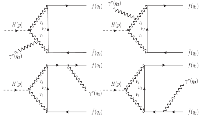
Figure 7: One-loop triangle and box diagrams with exchanging vector bosons $V_{i,j}$ in the loop.

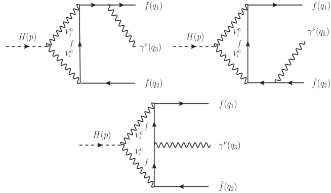
Figure 8: One-loop triangle and box diagrams with exchanging vector bosons $V^{0}_{i},V^{0}_{j}$ in the loop.

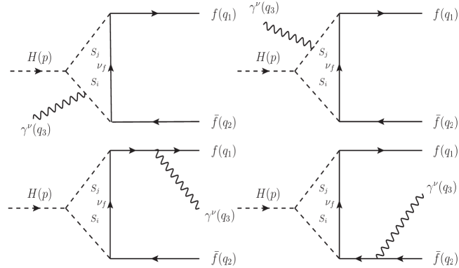
Figure 9: One-loop diagrams with exchanging charged scalar bosons $S_{i,j}$ in the loop.

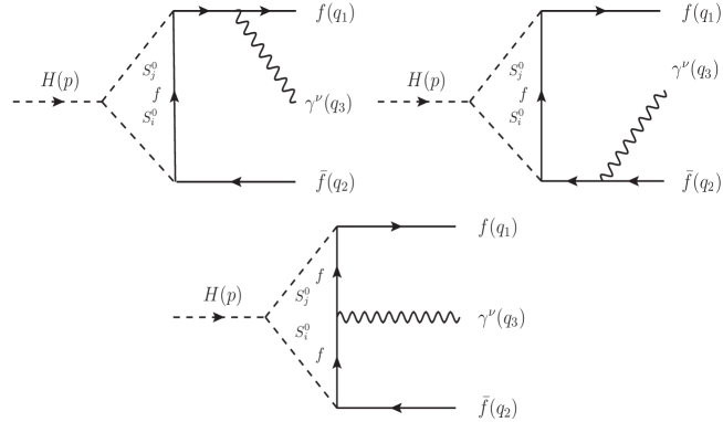
Figure 10: One-loop box diagrams with exchanging vector boson $S^{0}_{i,j}$ particles in loop.

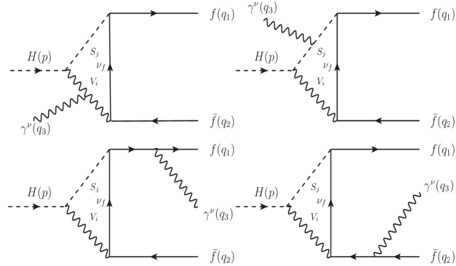
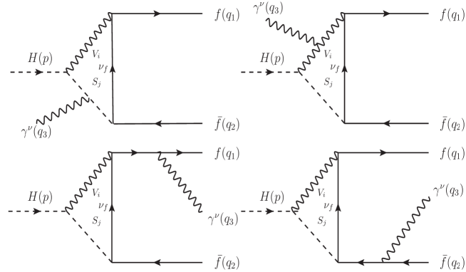
Figure 11: One-loop diagrams with exchanging vector boson $V_{i}$ and scalar boson $S_{j}$ particles in loop.

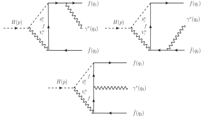
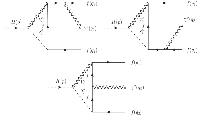
Figure 12: One-loop diagrams with exchanging vector boson $V^{0}_{i}$ and scalar boson $S_{j}^{0}$ particles in loop.

$$F_{1,L}^{\text{Non-$V_{k}^{0*}$}}|_{V_{i},V_{j}} = \dfrac{eQ_{V}}{16\pi^{2}}\sum\limits_{V_{i},V_{j}}\dfrac{g_{HV_{i}V_{j}}\,g_{V_{i}f\nu_{f}}^{L}\,g_{V_{j}f\nu_{f}}^{L}}{M_{V_{i}}^{2}M_{V_{j}}^{2}}\times$$

$$\times\Bigg{\{}-2M_{V_{i}}^{2}\Big{[}C_{0}(0,q_{12},M_{H}^{2},M_{V_{i}}^{2},M_{V_{i}}^{2},M_{V_{j}}^{2})+C_{0}(q_{12},0,M_{H}^{2},M_{V_{i}}^{2},M_{V_{j}}^{2},M_{V_{j}}^{2})\Big{]}$$

$$-(M_{H}^{2}+M_{V_{i}}^{2}+M_{V_{j}}^{2})\Big{\{}\Big{[}C_{22}+C_{12}\Big{]}(0,q_{12},M_{H}^{2},M_{V_{i}}^{2},M_{V_{i}}^{2},M_{V_{j}}^{2})$$

$$\hskip 142.26378pt+\Big{[}C_{22}+C_{12}\Big{]}(q_{12},0,M_{H}^{2},M_{V_{i}}^{2},M_{V_{j}}^{2},M_{V_{j}}^{2})\Big{\}}$$

$$-(M_{H}^{2}+3M_{V_{i}}^{2}-M_{V_{j}}^{2})\Big{[}C_{2}(0,q_{12},M_{H}^{2},M_{V_{i}}^{2},M_{V_{i}}^{2},M_{V_{j}}^{2})$$

$$\hskip 156.49014pt+C_{2}(q_{12},0,M_{H}^{2},M_{V_{i}}^{2},M_{V_{j}}^{2},M_{V_{j}}^{2})\Big{]}$$

$$+2(M_{V_{j}}^{2}-M_{V_{i}}^{2})C_{1}(q_{12},0,M_{H}^{2},M_{V_{i}}^{2},M_{V_{j}}^{2},M_{V_{j}}^{2})$$

$$+(8-2d)M_{V_{i}}^{2}M_{V_{j}}^{2}\Big{[}D_{3}(0,0,0,M_{H}^{2};q_{12},q_{13},M_{V_{i}}^{2},0,M_{V_{j}}^{2},M_{V_{j}}^{2})$$

$$\hskip 99.58464pt+D_{3}(0,0,0,M_{H}^{2};q_{23},q_{12},M_{V_{i}}^{2},M_{V_{i}}^{2},0,M_{V_{j}}^{2}))\Big{]}$$

$$+(4-2d)M_{V_{i}}^{2}M_{V_{j}}^{2}\Big{\{}\Big{[}D_{33}+D_{23}+D_{13}\Big{]}(0,0,0,M_{H}^{2};q_{23},q_{12},M_{V_{i}}^{2},M_{V_{i}}^{2},0,M_{V_{j}}^{2})$$

$$\hskip 99.58464pt+\Big{[}D_{33}+D_{23}\Big{]}(0,0,0,M_{H}^{2};q_{12},q_{13},M_{V_{i}}^{2},0,M_{V_{j}}^{2},M_{V_{j}}^{2})\Big{\}}$$

$$+4M_{V_{i}}^{2}M_{V_{j}}^{2}D_{2}(0,0,0,M_{H}^{2};q_{12},q_{13},M_{V_{i}}^{2},0,M_{V_{j}}^{2},M_{V_{j}}^{2})\Bigg{\}},$$

$$F_{1,R}^{\text{Non-$V_{k}^{0*}$}}|_{V_{i},V_{j}} = F_{1,L}^{\text{Non-$V_{k}^{0*}$}}|_{V_{i},V_{j}}\Big{(}g_{V_{i}f\nu_{f}}^{L}\rightarrow g_{V_{i}f\nu_{f}}^{R};\;g_{V_{j}f\nu_{f}}^{L}\rightarrow g_{V_{j}f\nu_{f}}^{R}\Big{)},$$ (24)

$$F_{2,L}^{\text{Non-$V_{k}^{0*}$}}|_{V_{i},V_{j}} = F_{1,L}^{\text{Non-$V_{k}^{0*}$}}|_{V_{i},V_{j}}\Big{(}\{q_{13},q_{23}\}\rightarrow\{q_{23},q_{13}\}\Big{)},$$ (25)

$$F_{2,R}^{\text{Non-$V_{k}^{0*}$}}|_{V_{i},V_{j}} = F_{2,L}^{\text{Non-$V_{k}^{0*}$}}|_{V_{i},V_{j}}\Big{(}g_{V_{i}f\nu_{f}}^{L}\rightarrow g_{V_{i}f\nu_{f}}^{R};\;g_{V_{j}f\nu_{f}}^{L}\rightarrow g_{V_{j}f\nu_{f}}^{R}\Big{)}.$$ (26)

We find that the result is presented in terms of $C$- and $D$-functions up to $D_{33}$-coefficients. The reason for this fact is explained as follows. Due to the exchange of vector boson in the loop, we have to handle with tensor one-loop integrals with rank $R\geq 3$ in the amplitude of each diagram. However, they are cancelled out after summing all diagrams. As a result, the total amplitude is only expressed in terms of tensor integrals with $R\leq 2$ that causes of leading the results.

For neutral vector boson $V^{0}_{i},V^{0}_{j}$ internal lines in the loop diagrams (seen Fig. 8), the corresponding form factors are obtained

$$F_{1,L}^{\text{Non-$V_{k}^{0*}$}}|_{V^{0}_{i},V^{0}_{j}} = \dfrac{eQ_{f}}{16\pi^{2}}\sum\limits_{V^{0}_{i},V^{0}_{j}}g_{HV^{0}_{i}V^{0}_{j}}\;g_{V^{0}_{i}ff}^{L}\;g_{V^{0}_{j}ff}^{L}\times$$

$$\times\Big{\{}(4-2d)\big{[}D_{33}+D_{23}\big{]}+(8-2d)D_{3}\Big{\}}(0,0,0,M_{H}^{2},q_{23},q_{13},M_{V^{0}_{i}}^{2},0,0,M_{V^{0}_{j}}^{2}),$$

$$F_{1,R}^{\text{Non-$V_{k}^{0*}$}}|_{V^{0}_{i},V^{0}_{j}} = F_{1,L}^{\text{Non-$V_{k}^{0*}$}}|_{V^{0}_{i},V^{0}_{j}}\Big{(}g_{V^{0}_{i}ff}^{L}\rightarrow g_{V^{0}_{i}ff}^{R};\;g_{V^{0}_{j}ff}^{L}\rightarrow g_{V^{0}_{j}ff}^{R}\Big{)},$$ (28)

$$F_{2,L}^{\text{Non-$V_{k}^{0*}$}}|_{V^{0}_{i},V^{0}_{j}} = F_{1,L}^{\text{Non-$V_{k}^{0*}$}}|_{V^{0}_{i},V^{0}_{j}}\Big{(}\{q_{13},q_{23}\}\rightarrow\{q_{23},q_{13}\}\Big{)},$$ (29)

$$F_{2,R}^{\text{Non-$V_{k}^{0*}$}}|_{V^{0}_{i},V^{0}_{j}} = F_{2,L}^{\text{Non-$V_{k}^{0*}$}}|_{V^{0}_{i},V^{0}_{j}}\Big{(}g_{V^{0}_{i}ff}^{L}\rightarrow g_{V^{0}_{i}ff}^{R};\;g_{V^{0}_{j}ff}^{L}\rightarrow g_{V^{0}_{j}ff}^{R}\Big{)}.$$ (30)

Next, we also consider one-loop diagrams with having charged scalar bosons $S_{i,j}$ internal lines (shown in Fig. 9). The results read

$$F_{1,L}^{\text{Non-$V_{k}^{0*}$}}|_{S_{i},S_{j}} = \dfrac{eQ_{S}}{8\pi^{2}}\sum\limits_{S_{i},S_{j}}g_{HS_{i}S_{j}}\,g_{S_{i}f\nu_{f}}^{R}\,g_{S_{j}f\nu_{f}}^{R}\times$$

$$\times\Bigg{\{}\Big{[}D_{33}+D_{23}+D_{3}\Big{]}(0,0,0,M_{H}^{2};q_{12},q_{13},M_{S_{i}}^{2},0,M_{S_{j}}^{2},M_{S_{j}}^{2})$$

$$\hskip 8.5359pt+\Big{[}D_{33}+D_{23}+D_{13}+D_{3}\Big{]}(0,0,0,M_{H}^{2};q_{23},q_{12},M_{S_{i}}^{2},M_{S_{i}}^{2},0,M_{S_{j}}^{2})\Bigg{\}},$$

$$F_{1,R}^{\text{Non-$V_{k}^{0*}$}}|_{S_{i},S_{j}} = F_{1,L}^{\text{Non-$V_{k}^{0*}$}}|_{S_{i},S_{j}}\Big{(}g_{S_{i}f\nu_{f}}^{R}\rightarrow g_{S_{i}f\nu_{f}}^{L};\;g_{S_{j}f\nu_{f}}^{R}\rightarrow g_{S_{j}f\nu_{f}}^{L}\Big{)},$$ (32)

$$F_{2,L}^{\text{Non-$V_{k}^{0*}$}}|_{S_{i},S_{j}} = F_{1,L}^{\text{Non-$V_{k}^{0*}$}}|_{S_{i},S_{j}}\Big{(}\{q_{13},q_{23}\}\rightarrow\{q_{23},q_{13}\}\Big{)},$$ (33)

$$F_{2,R}^{\text{Non-$V_{k}^{0*}$}}|_{S_{i},S_{j}} = F_{2,L}^{\text{Non-$V_{k}^{0*}$}}|_{S_{i},S_{j}}\Big{(}g_{S_{i}f\nu_{f}}^{R}\rightarrow g_{S_{i}f\nu_{f}}^{L};\;g_{S_{j}f\nu_{f}}^{R}\rightarrow g_{S_{j}f\nu_{f}}^{L}\Big{)}.$$ (34)

Furthermore, one also has the contributions of neutral scalar boson $S^{0}_{i,j}$ exchanging in the loop diagrams (as described in Fig. 10). Analytic results for the form factors then read

$$F_{1,L}^{\text{Non-$V_{k}^{0*}$}}|_{S^{0}_{i},S^{0}_{j}} = -\dfrac{eQ_{f}}{8\pi^{2}}\sum\limits_{S^{0}_{i},S^{0}_{j}}\,g_{HS^{0}_{i}S^{0}_{j}}\,g_{S^{0}_{i}ff}^{L}\,g_{S^{0}_{j}ff}^{R}\times$$

$$\times\Big{[}D_{33}+D_{23}+D_{3}\Big{]}(0,0,0,M_{H}^{2};q_{23},q_{13};M_{S^{0}_{i}}^{2},0,0,M_{S^{0}_{j}}^{2}),$$

$$F_{1,R}^{\text{Non-$V_{k}^{0*}$}}|_{S^{0}_{i},S^{0}_{j}} = F_{1,L}^{\text{Non-$V_{k}^{0*}$}}|_{S^{0}_{i},S^{0}_{j}}\Big{(}g_{S^{0}_{i}ff}^{L}\rightarrow g_{S^{0}_{i}ff}^{R};\;g_{S^{0}_{j}ff}^{R}\rightarrow g_{S^{0}_{j}ff}^{L}\Big{)},$$ (36)

$$F_{2,L}^{\text{Non-$V_{k}^{0*}$}}|_{S^{0}_{i},S^{0}_{j}} = F_{1,L}^{\text{Non-$V_{k}^{0*}$}}|_{S^{0}_{i},S^{0}_{j}}\Big{(}\{q_{13},q_{23}\}\rightarrow\{q_{23},q_{13}\}\Big{)},$$ (37)

$$F_{2,R}^{\text{Non-$V_{k}^{0*}$}}|_{S^{0}_{i},S^{0}_{j}} = F_{2,L}^{\text{Non-$V_{k}^{0*}$}}|_{S^{0}_{i},S^{0}_{j}}\Big{(}g_{S^{0}_{i}ff}^{L}\rightarrow g_{S^{0}_{i}ff}^{R};\;g_{S^{0}_{j}ff}^{R}\rightarrow g_{S^{0}_{j}ff}^{L}\Big{)}.$$ (38)

We now consider non-$V_{k}^{*0}$ pole one-loop diagrams with mixing of scalar $S_{j}$ (or $S_{j}^{0}$) and $V_{i}(V^{0}_{i})$ exchanging in the loop. The diagrams are depicted in Figs. 11,  12. The calculations are performed as same procedure. We finally find that these contributions are proportional to $m_{f}$. As a result, in the limit of $m_{f}\rightarrow 0$, one confirms that

$$F_{k,L}^{\text{Non-$V_{k}^{0*}$}}|_{V_{i},S_{j}}=F_{k,R}^{\text{Non-$V_{k}^{0*}$}}|_{V_{i},S_{j}} = 0,$$ (39)

$$F_{k,L}^{\text{Non-$V_{k}^{0*}$}}|_{V^{0}_{i},S^{0}_{j}}=F_{k,R}^{\text{Non-$V_{k}^{0*}$}}|_{V^{0}_{i},S^{0}_{j}} = 0.$$ (40)

for $k=1,2$.

We verify the ultraviolet finiteness of the results. We find that the UV-divergent parts of all the above form factors come from all $B$-functions. While $C$- and $D$-functions in this papers are UV-finite. Higher rank tensor $B$-functions can be reduced into $B_{0}$ and $A_{0}$. We verify that the sum of all $B$-functions gives a UV-finite result. As a result, all the form factors are UV-finite (seen our previous paper [45] for example).

Having the correctness form factors for the decay processes, the decay rate is given by [20]:

$$\dfrac{d\Gamma}{dq_{12}q_{13}}=\dfrac{q_{12}}{512\pi^{3}M_{H}^{3}}\Big{[}q_{13}^{2}(|F_{1,R}|^{2}+|F_{2,R}|^{2})+q_{23}^{2}(|F_{1,L}|^{2}+|F_{2,L}|^{2})\Big{]}.$$ (41)

Taking the above integrand over $0\leq q_{12}\leq M_{H}^{2}$ and $0\leq q_{13}\leq M_{H}^{2}-q_{12}$, one gets the total decay rates. In the next subsection, we show typical examples which we apply our analytical results for $H\rightarrow f\bar{f}\gamma$ to the Standard Model, the $U(1)_{B-L}$ extension of the SM, THDM. Phenomenological results for the decay channels of the mentioned models also studied with using the present parameters at the LHC.

4 Applications

We are going to apply the above results to the standard model and several BSMs such as the $U(1)_{B-L}$ extension of the SM, THDM. For phenomenological analyses, we use the following input parameters: $\alpha=1/137.035999084$, $M_{Z}=91.1876$ GeV, $\Gamma_{Z}=2.4952$ GeV, $M_{W}=80.379$ GeV, $M_{H}=125.1$ GeV, $m_{\tau}=1.77686$ GeV, $m_{t}=172.76$ GeV, $m_{b}=4.18$ GeV, $m_{s}=0.93$ GeV and $m_{c}=1.27$ GeV. Depending on the models under consideration, the input values for new parameters are then shown.

4.1 Standard model

We first reduce our result to the case of the standard model. In this case, we have $V_{i},V_{j}\rightarrow W^{+},W^{-}$, $V_{k}^{0}\rightarrow Z,\gamma$. All couplings relating to the decay channels $H\rightarrow f\bar{f}\gamma$ in the SM are replaced as in Table 1.

Vertices	Couplings
$g_{HV_{i}V_{j}}$	$eM_{W}/s_{W}$
$g_{V^{0}_{k}V_{i}V_{j}}$	$e\;c_{W}/s_{W}$
$g_{V^{0}_{k}AV_{i}V_{j}}$	$e^{2}\;c_{W}/s_{W}$
$g_{V^{0}_{k}\nu_{f}\nu_{f}}^{L}$	$e/(2s_{W}c_{W})$
$g_{V^{0}_{k}\nu_{f}\nu_{f}}^{R}$	$0$
$g_{Hf_{i}f_{j}}^{L,R}$	$e\;m_{f}/(2s_{W}\;M_{W})$
$g_{V^{0}_{k}f_{i}f_{j}}^{L}$	$e(T_{3}^{f}-Q_{f}\;s^{2}_{W})/(s_{W}\;c_{W})$
$g_{V^{0}_{k}f_{i}f_{j}}^{R}$	$-eQ_{f}s_{W}/c_{W}$
$g_{V_{i}f\nu_{f}}^{L}$	$e/(\sqrt{2}\;s_{W})$
$g_{V_{i}f\nu_{f}}^{R}$	$0$

Table 1: All the couplings involving the decay processes $H\rightarrow f\bar{f}\gamma$ in the SM.

In the SM, the form factors are obtained by taking the contributions of Eqs. (3.1, 3.1, 3.2, 3.2). Using the above couplings, we then get a compact expression for the form factors as follows:

$$F_{2L} = \dfrac{\alpha^{2}m_{t}^{2}}{3s_{W}M_{W}}\Bigg{[}\dfrac{16}{q_{12}}+\dfrac{2(8s_{W}^{2}-3)}{es_{W}c_{W}}\;\dfrac{g_{Zff}^{L}}{q_{12}-M_{Z}^{2}+i\Gamma_{Z}M_{Z}}\Bigg{]}\times$$

$$\hskip 19.91684pt\times\Bigg{\{}4\Big{(}C_{22}+C_{12}+C_{2}\Big{)}+C_{0}\Bigg{\}}(0,q_{12},M_{H}^{2},m_{t}^{2},m_{t}^{2},m_{t}^{2})$$

$$+\dfrac{\alpha^{2}}{s_{W}M_{W}^{3}}\Bigg{[}\dfrac{1}{q_{12}}-\dfrac{c_{W}}{es_{W}}\dfrac{g_{Zff}^{L}}{q_{12}-M_{Z}^{2}+i\Gamma_{Z}M_{Z}}\Bigg{]}\times$$

$$\hskip 19.91684pt\times\Bigg{\{}\Big{[}-M_{H}^{2}\Big{(}B_{1}+3B_{11}+2B_{111}\Big{)}-2\Big{(}B_{00}+2B_{001}\Big{)}\Big{]}(M_{H}^{2},M_{W}^{2},M_{W}^{2})$$

$$+\Big{[}4M_{W}^{2}\Big{(}q_{12}-M_{H}^{2}\Big{)}+2M_{H}^{2}q_{12}+8(1-d)M_{W}^{4}\Big{]}\times$$

$$\hskip 85.35826pt\times\Big{(}C_{22}+C_{12}+C_{2}\Big{)}(0,q_{12},M_{H}^{2},M_{W}^{2},M_{W}^{2},M_{W}^{2})$$

$$+4M_{W}^{2}(q_{12}-4M_{W}^{2})C_{0}(0,q_{12},M_{H}^{2},M_{W}^{2},M_{W}^{2},M_{W}^{2})\Bigg{\}}$$

$$+\dfrac{\alpha}{4\pi s_{W}M_{W}^{3}}\Big{(}g_{Wf\nu_{f}}^{L}\Big{)}^{2}\times$$

$$\hskip 19.91684pt\times\Bigg{\{}(-M_{H}^{2}-2M_{W}^{2})\Big{[}\Big{(}C_{12}+C_{11}+C_{1}\Big{)}(M_{H}^{2},0,q_{12},M_{W}^{2},M_{W}^{2},M_{W}^{2})$$

$$\hskip 122.34692pt+\Big{(}C_{12}+C_{11}+C_{1}\Big{)}(M_{H}^{2},q_{12},0,M_{W}^{2},M_{W}^{2},M_{W}^{2})\Big{]}$$

$$-2M_{W}^{2}\Big{[}C_{0}(M_{H}^{2},0,q_{12},M_{W}^{2},M_{W}^{2},M_{W}^{2})+C_{0}(M_{H}^{2},q_{12},0,M_{W}^{2},M_{W}^{2},M_{W}^{2})\Big{]}$$

$$+2M_{W}^{4}(2-d)\Big{[}\Big{(}D_{13}+D_{12}+D_{11}\Big{)}(M_{H}^{2},0,0,0;q_{12},q_{13},M_{W}^{2},M_{W}^{2},M_{W}^{2},0)$$

$$+\Big{(}D_{23}+D_{22}+D_{13}+2D_{12}+D_{11}\Big{)}(M_{H}^{2},0,0,0;q_{23},q_{12},M_{W}^{2},M_{W}^{2},0,M_{W}^{2})\Big{]}$$

$$-4M_{W}^{4}\Big{[}\Big{(}D_{3}+D_{2}+D_{0}\Big{)}(M_{H}^{2},0,0,0;q_{12},q_{13},M_{W}^{2},M_{W}^{2},M_{W}^{2},0)$$

$$\hskip 113.81102pt+D_{0}(M_{H}^{2},0,0,0;q_{23},q_{12},M_{W}^{2},M_{W}^{2},0,M_{W}^{2})\Big{]}$$

$$-2dM_{W}^{4}\Big{[}\Big{(}D_{2}+D_{1}\Big{)}(M_{H}^{2},0,0,0;q_{23},q_{12},M_{W}^{2},M_{W}^{2},0,M_{W}^{2})$$

$$\hskip 113.81102pt+D_{1}(M_{H}^{2},0,0,0;q_{12},q_{13},M_{W}^{2},M_{W}^{2},M_{W}^{2},0)\Big{]}\Bigg{\}}$$

$$+\dfrac{\alpha M_{W}}{2\pi c_{W}^{2}s_{W}}\Big{(}g_{Zff}^{L}\Big{)}^{2}\Bigg{\{}(d-2)\times$$

$$\hskip 28.45274pt\times\Big{[}D_{23}+D_{22}+D_{13}+2D_{12}+D_{11}\Big{]}(M_{H}^{2},0,0,0;q_{23},q_{13},M_{Z}^{2},M_{Z}^{2},0,0)$$

$$\hskip 28.45274pt+\Big{[}d\Big{(}D_{2}+D_{1}\Big{)}+2\Big{(}D_{3}+D_{0}\Big{)}\Big{]}(M_{H}^{2},0,0,0;q_{23},q_{13},M_{Z}^{2},M_{Z}^{2},0,0)\Bigg{\}}.$$

Where some coupling constants relate in this representation like $g_{Wf\nu_{f}}^{L}=e/(\sqrt{2}s_{W})$, $g_{Zff}^{L}=e(2s_{W}^{2}-1)/(2c_{W}s_{W})$ and $g_{Wf\nu_{f}}^{R}=0$, $g_{Zff}^{R}=es_{W}/c_{W}$.

Other form factors can be obtained as follows.

$$F_{1L} = F_{2L}\Big{(}\{q_{13},q_{23}\}\rightarrow\{q_{23},q_{13}\}\Big{)},$$ (43)

$$F_{kR} = F_{kL}\Big{(}g_{Wf\nu_{f}}^{L}\rightarrow g_{Wf\nu_{f}}^{R};g_{Zff}^{L}\rightarrow g_{Zff}^{R}\Big{)}$$ (44)

for $k=1,2$.

It is stress that we derive alternative results for the form factors of $H\rightarrow f\bar{f}\gamma$ in the SM in comparison with previous works. Because our analytic results in this paper are computed in the unitary. Thus, our formulas may get different forms in comparison with the results in [20] which have calculated in $R_{\xi}$-gauge. In this paper, we perform cross-check our results with [20] by numerical tests. The numerical results for this check are shown in Table 2. We find that our results are in good agreement with the ones in [20] with more than $10$ digits.

$(q_{12},q_{13})$	This work	Ref. [20]
$(100,200)$	$9.62231539663501\cdot 10^{-8}$	$9.62231539662956\cdot 10^{-8}$
	$-3.501515874673991\cdot 10^{-10}\,i$	$-3.501515874674078\cdot 10^{-10}\,i$
$(-100,200)$	$-9.95227151085161\cdot 10^{-8}$	$-9.95227151084899\cdot 10^{-8}$
	$-3.531494528007124\cdot 10^{-10}\,i$	$-3.531494528006995\cdot 10^{-10}\,i$
$(100,-200)$	$9.62360254230002\cdot 10^{-8}$	$9.62360254229717\cdot 10^{-8}$
	$-3.597907189717628\cdot 10^{-10}\,i$	$-3.597907189717582\cdot 10^{-10}\,i$
$(-100,-200)$	$-9.95098785515085\cdot 10^{-8}$	$-9.95098785514946\cdot 10^{-8}$
	$-3.622848558573573\cdot 10^{-10}\,i$	$-3.622848558573332\cdot 10^{-10}\,i$

Table 2: Numerical checks for form factor $F_{2L}$ in this work with $b_{1}$ in $A2$ of [20].

We also generate the decay widths for $H\rightarrow e\bar{e}\gamma$ and cross-check our results with [13]. The results are presented in Table 3. For this test, we adjust the input parameters and apply all cuts as same in [13]. In the Table 3, the parameter $k$ is taken account which come from the kinematical cuts of the invariant masses $m_{ff},\;m_{f\gamma}$ as follows:

$$m_{ff}^{2},m_{f\gamma}^{2}\geq(kM_{H})^{2}.$$ (45)

We find that our results are in good agreement with the ones in [13].

$k$	This work	Ref. [13]
$0$	$0.576865$	$0.5782$
$0.1$	$0.242514$	$0.245$
$0.2$	$0.184121$	$0.1897$
$0.3$	$0.121368$	$0.1242$
$0.4$	$0.0572478$	$0.05844$

Table 3: Cross-check the results of the decay widths in this work with [13]

4.2 $U(1)_{B-L}$ extension of the SM

We refer to the appendix $B$ for reviewing briefly this model. In the appendix $B$, all couplings relating to the decay processes $H\rightarrow f\bar{f}\gamma$ are derived in $U(1)_{B-L}$ extension of the SM (seen Table 4). Apart from all particles in the SM, two additional neutral Higgs and a neutral gauge boson $Z^{\prime}$ which belongs to $U(1)_{B-L}$ gauge symmetry are taken into account in this model.

For phenomenological study, we have to include three new parameters such as the mixing angle $c_{\alpha}$, the $U(1)_{B-L}$ coupling $g^{\prime}_{1}$ and the mass of new gauge boson $M_{Z}^{\prime}$. In all the below results, we set $c_{\alpha}=0.3,0.7$ and $c_{\alpha}=1$ (this case is to the standard model). The mass of $Z^{\prime}$ is in the range of $600$ GeV $\leq M_{Z}^{\prime}\leq 1000$ GeV. The coupling $g^{\prime}_{1}$ is in $0.05\leq g_{1}^{\prime}\leq 0.5$.

We study the impact of the $U(1)_{B-L}$ extension of the SM on the differential decay widths as functions of $m_{ff}$ and $m_{f\gamma}$. The results are shown in the Fig. 13 with fixing $M_{Z}^{\prime}=1000$ GeV. In these figures, the solid line shows for the SM case by setting $c_{\alpha}=1$. While the dashed line presents for $c_{\alpha}=0.7$ and the dashed dot line is for $c_{\alpha}=0.3$. In the left figure, we observe photon pole at the lowest region of $m_{ff}$. The decay rates decrease up to $m_{ff}\sim 60$ GeV. They then grown up to $Z$-peak (the peak of $Z\rightarrow f\bar{f}$) which locates around $m_{ff}\sim 90$ GeV. Beyond the peak, the decay rates decrease rapidly. In the right figure, the decay widths increase up to peak of $m_{f\gamma}\sim 81$ GeV which is corresponding the photon recoil mass at $Z$-pole. They also decrease rapidly beyond the peak. It is interested to find that the contributions of $U(1)_{B-L}$ extension are sizable in both case of $c_{\alpha}=0.7,0.3$. These effects can be probed clearly at the future colliders.

$\begin{array}[]{cc}\dfrac{d\Gamma}{dm_{f\bar{f}}}&\dfrac{d\Gamma}{dm_{f\gamma}}\\ &\\ \includegraphics[width=227.62204pt,height=227.62204pt]{./U1/HFFG_U1_mll_Input_gBL_0.5_MZBL_1000_cA_SM_1.0_0.7_0.3.eps}&\includegraphics[width=227.62204pt,height=227.62204pt]{./U1/HFFG_U1_mlg_Input_gBL_0.5_MZBL_1000_cA_SM_1.0_0.7_0.3.eps}\\ \hskip 142.26378ptm_{ff}\;\text{[GeV]}&\hskip 142.26378ptm_{f\gamma}\;\text{[GeV]}\end{array}$

Figure 13: Differential of the decay width as functions of $m_{ff}$ and $m_{f\gamma}$

We next examine the decay widths as a function of $M_{Z}^{\prime}$. In this study, we change the mass of $Z^{\prime}$ boson as $800$ GeV $\leq M_{Z^{\prime}}\leq 1000$ GeV and set $c_{\alpha}=0.7$ (see Fig. 14), the dashed line shows for the case of $g^{\prime}_{1}=0.05$, the dot line presents for $g^{\prime}_{1}=0.2$ and the dashed dot line is for $g^{\prime}_{1}=0.5$. In all range of $M_{Z}^{\prime}$, we observe that the decay widths are proportional to $g_{1}^{\prime}$ (it is also confirmed later analyses). They also decrease with increasing $M_{Z}^{\prime}$. We conclude that the contributions from the $U(1)_{B-L}$ extension are massive and can be probed clearly at future colliders.

$\Gamma$ [KeV]

                                                                                       $M_{Z^{\prime}}$

Figure 14: The decay widths which are functions of $M_{Z}^{\prime}$

We finally discuss how the effect of $g^{\prime}_{1}$ on the decay widths (seen Fig. 15). In these figures, we set $M_{Z^{\prime}}=800$ GeV and $c_{\alpha}=0.3$ ($c_{\alpha}=0.7$) for the left figure (for the right figure) respectively. We find that the decay width are proportional to $g_{1}^{\prime}$.

$\begin{array}[]{cc}\Gamma\text{[KeV]}&\Gamma\text{[KeV]}\\ \includegraphics[width=227.62204pt,height=227.62204pt]{./U1/HFFG_U1_gBL_Input_cA_0.3_MZBL_800.eps}&\includegraphics[width=227.62204pt,height=227.62204pt]{./U1/HFFG_U1_gBL_Input_cA_0.7_MZBL_800.eps}\\ \hskip 142.26378ptg_{1}^{\prime}&\hskip 142.26378ptg_{1}^{\prime}\end{array}$

Figure 15: The decay widths are function of $g_{1}^{\prime}$

4.3 Two Higgs Doublet Model

For reviewing THDM, we refer the appendix $C$ for more detail. In this framework, the gauge sector is same the SM case. It means that we have $V_{i}=V_{j}=W$, $V_{k}^{0}=Z,\gamma$. In the Higgs sectors, one has additional charged Higgs $H^{+}$ and two neutral scalar CP even Higgs bosons $H_{1}^{0},H_{2}^{0}$, a CP odd Higgs $A$. All couplings relating to the decay processes $H\rightarrow f\bar{f}\gamma$ are shown in Table 5.

For the phenomenological results, we take $1\leq\tan\beta\leq 30$, $M_{H_{1}^{0}}=125.1$ GeV, $-900^{2}$ GeV² $\leq m_{12}^{2}\leq 900^{2}$ GeV², $340$ GeV $\leq M_{H^{\pm}}\leq 900$ GeV, $-\pi/2\leq\alpha\leq\pi/2$. We study the differential decay rates as a function of the invariant mass of leptons $m_{ff}$. We select $M_{H^{\pm}}=700$ GeV, $m_{12}^{2}=800^{2}$ GeV². The results are shown in Fig. 16. In this figure, the solid line shows for the SM case. The dashed line presents for the case of $\alpha=-0.4\pi$. The dashed dot line is for the case of $\alpha=0$. The dot line is for the case of $\alpha=0.4\pi$. From the top to bottom of the figure, we have the corresponding figure to $\tan\beta=5,10,15,25$. The decay rates are same behavior in previous cases, we observe photon pole at the lowest region of $m_{ff}$. They decrease from photon pole to the region of $m_{ff}\sim 60$ GeV and then grown up to $Z$-peak. Beyond the $Z$-peak, the decay rates decrease rapidly. The effect of THDM are also visible in all cases.

$\begin{array}[]{cc}\includegraphics[width=227.62204pt,height=227.62204pt]{./thdm/HFFG_C2HDM_DR_mll_tanb_5_alpha.eps}&\includegraphics[width=227.62204pt,height=227.62204pt]{./thdm/HFFG_C2HDM_DR_mll_tanb_10_alpha.eps}\\ \\ \includegraphics[width=227.62204pt,height=227.62204pt]{./thdm/HFFG_C2HDM_DR_mll_tanb_15_alpha.eps}&\includegraphics[width=227.62204pt,height=227.62204pt]{./thdm/HFFG_C2HDM_DR_mll_tanb_25_alpha.eps}\end{array}$

Figure 16: Differential decay rates as a function of the invariant mass of leptons $m_{ff}$ with changing $\alpha=-0.4\pi,0,0.4\pi$

We next change charged Higgs masses $M_{H^{\pm}}=400,600,800$ GeV and take $\alpha=0.4\pi$. From the top to bottom of the figure, we have the corresponding figure to the case of $\tan\beta=5,10,15,25$ (seen Fig. 17). The decay widths depend on $m_{ff}$ the same previous explanation. They are inversely proportional to the charged Higgs masses. We find that the effect of THDM are sizeable contributions in all the above cases. These effects can be discriminated clearly at future colliders.

$\begin{array}[]{cc}\includegraphics[width=227.62204pt,height=227.62204pt]{./thdm/HFFG_C2HDM_DR_mll_tanb_5_MCH.eps}&\includegraphics[width=227.62204pt,height=227.62204pt]{./thdm/HFFG_C2HDM_DR_mll_tanb_10_MCH.eps}\\ \\ \includegraphics[width=227.62204pt,height=227.62204pt]{./thdm/HFFG_C2HDM_DR_mll_tanb_15_MCH.eps}&\includegraphics[width=227.62204pt,height=227.62204pt]{./thdm/HFFG_C2HDM_DR_mll_tanb_25_MCH.eps}\end{array}$

Figure 17: Differential decay rates as a function of the invariant mass of leptons $m_{ff}$ with changing charged Higgs masses $M_{H^{\pm}}=400,600,800$ GeV.

5 Conclusions

We have performed the calculations for one-loop contributing to the decay processes $H\rightarrow f\bar{f}\gamma$ in the limit of $m_{f}\rightarrow 0$. In this computation, we have considered all possible contributions of additional heavy vector gauge bosons, heavy fermions, and charged (and also neutral) scalar particles which they may exchange in the loop diagrams. The analytic formulas are written in terms of Passarino-Veltman functions which they can be evaluated numerically by using the package LoopTools. The evaluations have then applied standard model, $U(1)_{B-L}$ extension of the SM, two Higgs doublet model. Phenomenological results of the decay processes for the above models have studied in detail. We find that the effects of new physics are sizable contributions and they can be probed at future colliders.

Acknowledgment:  This research is funded by Vietnam National Foundation for Science and Technology Development (NAFOSTED) under the grant number $103.01$-$2019.346$. K. H. Phan would like to thank Dr. L. T. Hue for helpful discussions.

Appendix A Tensor one-loop reductions

In this appendix, tensor one-loop reduction method in [44] is discussed briefly. First, the definition of one-loop one-, two-, three- and four-point tensor integrals with rank $R$ are as follows:

$$\{A;B;C;D\}^{\mu_{1}\mu_{2}\cdots\mu_{R}}=(\mu^{2})^{2-d/2}\int\frac{d^{d}k}{(2\pi)^{d}}\dfrac{k^{\mu_{1}}k^{\mu_{2}}\cdots k^{\mu_{R}}}{\{P_{1};P_{1}P_{2};P_{1}P_{2}P_{3};P_{1}P_{2}P_{3}P_{4}\}}.$$ (46)

In this formula, $P_{j}$ ($j=1,\cdots,4$) are the inverse Feynman propagators

$$P_{j}=(k+q_{j})^{2}-m_{j}^{2}+i\rho.$$ (47)

In this equation, we use $q_{j}=\sum\limits_{i=1}^{j}p_{i}$ with $p_{i}$ for the external momenta, and $m_{j}$ for internal masses in the loops. Dimensional regularization is performed in space-time dimension $d=4-2\varepsilon$. The parameter $\mu^{2}$ plays role of a renormalization scale. When the numerator of the integrands in Eq. (46) becomes $1$, one has the corresponding scalar one-loop functions (they are noted as $A_{0}$, $B_{0}$, $C_{0}$ and $D_{0}$). Explicit reduction formulas for one-loop one-, two-, three- and four-point tensor integrals up to rank $R=3$ are written as follows [44]. In particular, for two-point tensor integrals, the reduction formulas are:

$$A^{\mu} = 0,$$ (48)

$$A^{\mu\nu} = g^{\mu\nu}A_{00},$$ (49)

$$A^{\mu\nu\rho} = 0,$$ (50)

$$B^{\mu} = q^{\mu}B_{1},$$ (51)

$$B^{\mu\nu} = g^{\mu\nu}B_{00}+q^{\mu}q^{\nu}B_{11},$$ (52)

$$B^{\mu\nu\rho} = \{g,q\}^{\mu\nu\rho}B_{001}+q^{\mu}q^{\nu}q^{\rho}B_{111},$$ (53)

For three-point functions, one has

$$C^{\mu} = q_{1}^{\mu}C_{1}+q_{2}^{\mu}C_{2}=\sum\limits_{i=1}^{2}q_{i}^{\mu}C_{i},$$ (54)

$$C^{\mu\nu} = g^{\mu\nu}C_{00}+\sum\limits_{i,j=1}^{2}q_{i}^{\mu}q_{j}^{\nu}C_{ij},$$ (55)

$$C^{\mu\nu\rho} = \sum_{i=1}^{2}\{g,q_{i}\}^{\mu\nu\rho}C_{00i}+\sum_{i,j,k=1}^{2}q^{\mu}_{i}q^{\nu}_{j}q^{\rho}_{k}C_{ijk},$$ (56)

Similarly, tensor reduction formulas for four-point functions are given by

$$D^{\mu} = q_{1}^{\mu}D_{1}+q_{2}^{\mu}D_{2}+q_{3}^{\mu}D_{3}=\sum\limits_{i=1}^{3}q_{i}^{\mu}D_{i},$$ (57)

$$D^{\mu\nu} = g^{\mu\nu}D_{00}+\sum\limits_{i,j=1}^{3}q_{i}^{\mu}q_{j}^{\nu}D_{ij},$$ (58)

$$D^{\mu\nu\rho} = \sum_{i=1}^{3}\{g,q_{i}\}^{\mu\nu\rho}D_{00i}+\sum_{i,j,k=1}^{3}q^{\mu}_{i}q^{\nu}_{j}q^{\rho}_{k}D_{ijk}.$$ (59)

The short notation [44] $\{g,q_{i}\}^{\mu\nu\rho}$ is used as follows: $\{g,q_{i}\}^{\mu\nu\rho}=g^{\mu\nu}q^{\rho}_{i}+g^{\nu\rho}q^{\mu}_{i}+g^{\mu\rho}q^{\nu}_{i}$ in the above relations. The scalar coefficients $A_{00},B_{1},\cdots,D_{333}$ in the right hand sides of the above equations are so-called Passarino-Veltman functions  [44]. They have been implemented into LoopTools [46] for numerical computations.

Appendix B Review of $U(1)_{B-L}$ extension

In this appendix, we review briefly $U(1)_{B-L}$ extension [25]. This model follows gauge symmetry $SU(3)_{C}\otimes SU(2)_{L}\otimes U(1)_{Y}\otimes U(1)_{B-L}$. By including complex scalar $S$, general scalar potential is given by

$$V(\Phi,S) = m^{2}\Phi^{{\dagger}}\Phi+\lambda_{1}(\Phi^{{\dagger}}\Phi)^{2}+\mu^{2}|S|^{2}+\lambda_{2}|S|^{4}+\lambda_{3}\Phi^{{\dagger}}\Phi|S|^{2}.$$ (60)

In order to find mass spectrum of the scalar sector, we expand the scalar fields around their vacuum as follows:

$$\Phi=\begin{pmatrix}\phi^{+}\\ \dfrac{v_{\phi}+h+i\xi}{\sqrt{2}}\end{pmatrix},\quad S=\dfrac{v_{s}+h^{\prime}+i\xi^{\prime}}{\sqrt{2}}.$$ (61)

The Goldstone bosons $\phi^{\pm},\xi$ will give the masses of $W^{\pm}$ and $Z$ bosons. In unitary gauge, the mass eigenvalues of neutral Higgs are given:

$$\begin{pmatrix}h_{1}\\ h_{2}\end{pmatrix}=\begin{pmatrix}c_{\alpha}&-s_{\alpha}\\ s_{\alpha}&c_{\alpha}\\ \end{pmatrix}\begin{pmatrix}h\\ h^{\prime}\end{pmatrix}$$ (62)

with mixing angle

$$s_{2\alpha}=\sin 2\alpha=\dfrac{\lambda_{3}v_{\phi}v_{s}}{\sqrt{(\lambda_{1}v_{\phi}^{2}-\lambda_{2}v_{s}^{2})^{2}+(\lambda_{3}v_{\phi}v_{s})^{2}}}$$ (63)

After this transformation, masses of scalar Higgs are given

$$M^{2}_{h_{1}} = \lambda_{1}v_{\phi}^{2}+\lambda_{2}v_{s}^{2}-\sqrt{(\lambda_{1}v_{\phi}^{2}-\lambda_{2}v_{s}^{2})^{2}+(\lambda_{3}v_{\phi}v_{s})^{2}},$$ (64)

$$M^{2}_{h_{2}} = \lambda_{1}v_{\phi}^{2}+\lambda_{2}v_{s}^{2}+\sqrt{(\lambda_{1}v_{\phi}^{2}-\lambda_{2}v_{s}^{2})^{2}+(\lambda_{3}v_{\phi}v_{s})^{2}}.$$ (65)

For gauge boson masses, $W,Z$ and $Z^{\prime}$ bosons are obtained their masses by expanding the following kinematic terms

$$\mathcal{L}_{\text{gauge}}\rightarrow(D^{\mu}\Phi)^{+}D_{\mu}\Phi,\quad(D^{\mu}S)^{+}D_{\mu}S.$$ (66)

As a result, mass of $Z^{\prime}$ is $M_{Z^{\prime}}=2v_{s}g_{1}^{\prime}$.

The Yukawa interaction involving right-handed neutrinos are given:

$$\mathcal{L}_{Y} = -y^{d}_{jk}\bar{q}_{Lj}d_{Rk}\Phi-y^{u}_{jk}\bar{q}_{Lj}u_{Rk}i\sigma_{2}\Phi^{*}-y^{e}_{jk}\bar{l}_{Lj}e_{Rk}\Phi$$ (67)

$$-y^{\nu}_{jk}\bar{l}_{Lj}\nu_{Rk}i\sigma_{2}\Phi^{*}-y^{M}_{jk}\overline{(\nu_{R})}_{j}^{c}\nu_{Rk}\;S+\text{h.c}.$$

for $j,k=1,2,3$. The last term in this equation is Majorana mass terms for right-handed neutrinos. After the spontaneous breaking symmetry, the mass matrix of neutrinos is

$$M=\begin{pmatrix}0&m_{D}=\dfrac{(y^{\nu})^{*}}{\sqrt{2}}v_{\phi}\\ m_{D}^{T}&M=\sqrt{2}y^{M}v_{s}\\ \end{pmatrix}.$$ (68)

The diagonalization is obtained by the transformation

$$\text{diag}\Big{(}-\dfrac{(m^{i}_{D})^{2}}{M^{i}},M^{i}\Big{)}=\begin{pmatrix}\cos\alpha_{i}&-\sin\alpha_{i}\\ \sin\alpha_{i}&\cos\alpha_{i}\\ \end{pmatrix}\begin{pmatrix}0&m_{D}^{i}\\ m_{D}^{i}&M^{i}\\ \end{pmatrix}\begin{pmatrix}\cos\alpha_{i}&\sin\alpha_{i}\\ -\sin\alpha_{i}&\cos\alpha_{i}\\ \end{pmatrix}$$ (69)

for $i=1,2,3$ and $\alpha_{i}=\text{arcsin}(m_{D}^{i}/M^{i})$.

We show all relevant couplings in the decay under consider In the case of $\alpha_{i}\rightarrow 0$, all the couplings are shown in Table 4

Vertices	Couplings
$h_{1}(h_{2})f\bar{f}$	$-i\dfrac{c_{\alpha}(s_{\alpha})e\;m_{f}}{2M_{W}s_{W}}$
$Z^{\prime}_{\mu}f\bar{f}$	$iQ_{f}\;g^{\prime}_{1}\gamma_{\mu}$
$h_{1}(h_{2})W^{+}_{\mu}W^{-}_{\nu}$	$i\frac{eM_{W}}{s_{W}}\;c_{\alpha}(s_{\alpha})g_{\mu\nu}$
$h_{1}(h_{2})Z_{\mu}Z_{\nu})$	$i\frac{eM_{W}}{c_{W}^{2}\;s_{W}}\;c_{\alpha}(s_{\alpha})g_{\mu\nu}$
$h_{1}(h_{2})Z^{\prime}_{\mu}Z^{\prime}_{\nu})$	$-i4g^{\prime}_{1}M_{Z}^{\prime}\;s_{\alpha}(-c_{\alpha})g_{\mu\nu}$

Table 4: All the couplings involving the decay processes $H\rightarrow f\bar{f}\gamma$ in the $U(1)_{B-L}$ extension of the SM.

Appendix C Review of Two Higgs Doublet Model

Base on Ref. [27], we review briefly the two Higgs doublet model with breaking softly $Z_{2}$-symmetry. In this model, there are two scalar doublets $\Phi_{1},\Phi_{2}$ with hypercharge $Y=1/2$. Parts of Lagrangian extended from the SM are presented as follows:

$$\mathcal{L}=\mathcal{L}_{K}+\mathcal{L}_{Y}-V(\Phi_{1},\Phi_{2}).$$ (70)

Where the kinematic term is $\mathcal{L}_{K}$, the Yukawa part is $\mathcal{L}_{Y}$ and $V(\Phi_{1},\Phi_{2})$ is Higgs potential. First, the kinematic term is taken the form of

$$\mathcal{L}_{K}=\sum\limits_{k=1}^{2}\left(D_{\mu}\Phi_{k}\right)^{{\dagger}}\left(D^{\mu}\Phi_{k}\right)$$ (71)

with $D_{\mu}=\partial_{\mu}-igT^{a}W^{a}_{\mu}-i\frac{g^{\prime}}{2}B_{\mu}$. The Higgs potential with breaking the $Z_{2}$-symmetry is expressed:

$$V(\Phi_{1},\Phi_{2}) = \frac{1}{2}m_{11}^{2}\Phi_{1}^{{\dagger}}\Phi_{1}-m_{12}^{2}(\Phi_{1}^{{\dagger}}\Phi_{2}+\Phi_{2}^{{\dagger}}\Phi_{1})+\frac{1}{2}m_{22}^{2}\Phi_{2}^{{\dagger}}\Phi_{2}+\dfrac{\lambda_{1}}{2}\left(\Phi_{1}^{{\dagger}}\Phi_{1}\right)^{2}+\dfrac{\lambda_{2}}{2}\left(\Phi_{2}^{{\dagger}}\Phi_{2}\right)^{2}$$ (72)

$$+\lambda_{3}\left(\Phi_{1}^{{\dagger}}\Phi_{1}\right)\left(\Phi_{2}^{{\dagger}}\Phi_{2}\right)+\lambda_{4}\left(\Phi_{1}^{{\dagger}}\Phi_{2}\right)\left(\Phi_{2}^{{\dagger}}\Phi_{1}\right)+\frac{\lambda_{5}}{2}\left[\left(\Phi_{1}^{{\dagger}}\Phi_{2}\right)^{2}+\left(\Phi_{1}^{{\dagger}}\Phi_{2}\right)^{2}\right].$$

In this potential, $m_{12}^{2}$ plays role of soft broken scale of the $Z_{2}$-symmetry. The two scalar doublet fields can be parameterized as follows:

$$\Phi_{1}=\begin{pmatrix}\phi_{1}^{+}\\ \dfrac{v_{1}+\eta_{1}+i\xi_{1}}{\sqrt{2}}\end{pmatrix},\quad\Phi_{2}=\begin{pmatrix}\phi_{2}^{+}\\ \dfrac{v_{2}+\eta_{2}+i\xi_{2}}{\sqrt{2}}\end{pmatrix}.$$ (73)

We get a system equation for these parameters from the stationary conditions of the Higgs potential. The relations are shown as follows:

$$m_{11}^{2}-\mu^{2}\frac{v_{2}^{2}}{v^{2}}+\frac{\lambda_{1}}{2}v_{1}^{2}+\frac{\lambda_{345}}{2}v_{2}^{2} = 0,$$ (74)

$$m_{22}^{2}-\mu^{2}\frac{v_{1}^{2}}{v^{2}}+\frac{\lambda_{2}}{2}v_{2}^{2}+\frac{\lambda_{345}}{2}v_{1}^{2} = 0.$$ (75)

Where $v^{2}=v_{1}^{2}+v_{2}^{2}$ is fixed at electroweak scale or $v=(\sqrt{2}G_{F})^{-1/2}=246$ GeV and new parameter $\mu^{2}$ is defined as $\mu^{2}=\frac{v^{2}}{v_{1}v_{2}}m_{12}^{2}$. The shorten notation is $\lambda_{345}=\lambda_{3}+\lambda_{4}+\lambda_{5}$. The mixing angle is given $t_{\beta}=\tan\beta=v_{2}/v_{1}$. The mass terms of the Higgs potential $V_{mass}$ can be expressed as:

$$V_{mass} = (\phi^{+}_{1},\phi^{+}_{2})R_{\beta}\begin{pmatrix}0&0\\ 0&M^{2}_{H^{+}}\\ \end{pmatrix}R_{\beta}^{-1}\begin{pmatrix}\phi_{1}^{+}\\ \phi_{2}^{+}\end{pmatrix}+\frac{1}{2}(\xi_{1},\xi_{2})R_{\beta}\begin{pmatrix}0&0\\ 0&M^{2}_{A}\\ \end{pmatrix}R_{\beta}^{-1}\begin{pmatrix}\xi_{1}\\ \xi_{2}\\ \end{pmatrix}$$ (76)

$$+\frac{1}{2}(\eta_{1},\eta_{2})R_{\beta}\begin{pmatrix}M^{2}_{H_{2}^{0}}&0\\ 0&M^{2}_{H_{1}^{0}}\\ \end{pmatrix}R_{\beta}^{-1}\begin{pmatrix}\eta_{1}\\ \eta_{2}\end{pmatrix}.$$

Here diagonalized matrix of neutral mass is defined as

$$\text{diag}(M^{2}_{H_{2}^{0}},M^{2}_{H_{1}^{0}})=R_{\alpha}\mathcal{M}^{2}R_{\alpha}^{T},\quad\text{with}\quad(\mathcal{M}^{2})_{ij}=\dfrac{\partial^{2}V}{\partial{\eta_{i}}\partial{\eta_{j}}}.$$ (77)

The mass eigenstates can be then expressed as follows:

$$\begin{pmatrix}G^{+}\\ H^{+}\end{pmatrix}=R_{\beta}^{-1}\begin{pmatrix}\phi_{1}^{+}\\ \phi_{2}^{+}\end{pmatrix},\quad\begin{pmatrix}G^{0}\\ A\end{pmatrix}=R_{\beta}^{-1}\begin{pmatrix}\xi_{1}\\ \xi_{2}\end{pmatrix},\quad\begin{pmatrix}H_{2}^{0}\\ H_{1}^{0}\end{pmatrix}=R_{\alpha}^{-1}R_{\beta}^{-1}\begin{pmatrix}\eta_{1}\\ \eta_{2}\end{pmatrix}$$ (78)

where

$$R_{\beta}=\begin{pmatrix}c_{\beta}&s_{\beta}\\ -s_{\beta}&c_{\beta}\\ \end{pmatrix},\quad R_{\alpha}=\begin{pmatrix}c_{\alpha}&s_{\alpha}\\ -s_{\alpha}&c_{\alpha}\\ \end{pmatrix}$$ (79)

with $-\pi/2\leq\alpha\leq\pi/2$. In the unitary gauge, it is well-known that $G^{+}$ and $G^{0}$ are massless Goldstone bosons will become the longitudinal polarization of $W^{+}$ and $Z^{0}$. The remains $H^{\pm}$, $A$ and $H^{0}_{1,2}$ become the charged Higgs bosons, a CP-odd Higgs boson and CP-even Higgs bosons respectively. The masses of these scalar bosons are given by

$$M^{2}_{H^{\pm}} = \mu^{2}-\frac{v^{2}}{2}(\lambda_{4}+\lambda_{5}),$$ (80)

$$M^{2}_{A} = \mu^{2}-v^{2}\lambda_{5},$$ (81)

$$M^{2}_{H^{0}_{1}} = s_{\alpha}^{2}\mathcal{M}^{2}_{11}-2s_{\alpha}c_{\alpha}\mathcal{M}^{2}_{12}+c_{\alpha}^{2}\mathcal{M}^{2}_{22},$$ (82)

$$M^{2}_{H^{0}_{2}} = c_{\alpha}^{2}\mathcal{M}^{2}_{11}+2s_{\alpha}c_{\alpha}\mathcal{M}^{2}_{12}+s_{\alpha}^{2}\mathcal{M}^{2}_{22}.$$ (83)

From the Higgs potential in Eq. (72) with the stationary conditions in (74), we have $7$ parameters. They are

$$\Big{\{}\lambda_{1,2,3,4,5},t_{\beta},m_{12}^{2}\Big{\}}.$$ (84)

For phenomenological analyses, the above parameters are transferred to the following parameters:

$$\Big{\{}M^{2}_{H^{+}},M^{2}_{A},M^{2}_{H^{0}_{1}},M^{2}_{H^{0}_{2}},\alpha,t_{\beta},m_{12}^{2}\Big{\}}.$$ (85)

All the couplings involving the decay processes $H\rightarrow f\bar{f}\gamma$ are derived in this appendix. In general, we can consider the lightest Higgs boson $H_{1}^{0}$ is the SM like-Higgs boson. In Table 5, all the couplings are shown in detail.

Vertices	Couplings
$H_{1}^{0}W^{+}_{\mu}W^{-}_{\nu}$	$i\frac{2M_{W}^{2}}{v}s_{(\beta-\alpha)}g_{\mu\nu}$
$H_{1}^{0}Z_{\mu}Z_{\nu}$	$i\frac{2M_{Z}^{2}}{v}s_{(\beta-\alpha)}g_{\mu\nu}$
$H_{1}^{0}(p)H^{\pm}(q)W^{\mp}_{\mu}$	$\mp i\frac{M_{W}}{v}c_{(\beta-\alpha)}\;(p-q)_{\mu}$
$H^{+}(p)H^{-}(q)A_{\mu}$	$i\frac{2M_{W}}{v}s_{W}\;(p-q)_{\mu}$
$H^{+}(p)H^{-}(q)Z_{\mu}$	$i\frac{M_{Z}}{v}c_{2W}\;(p-q)_{\mu}$
$H_{1}^{0}H^{+}H^{-}$	$\frac{i}{v}\Big{[}(2\mu^{2}-2M_{H^{\pm}}^{2}-M^{2}_{H^{0}_{1}})s_{(\beta-\alpha)}+2(\mu^{2}-M^{2}_{H^{0}_{1}})\text{cot}2\beta\;c_{(\beta-\alpha)}\Big{]}$
$H^{+}H^{-}A_{\mu}A_{\nu}$	$2ie^{2}\;g_{\mu\nu}$
$H^{+}H^{-}Z_{\mu}A_{\nu}$	$ieg\frac{c_{2W}}{c_{W}}\;g_{\mu\nu}$

Table 5: All the couplings involving the decay processes $H\rightarrow f\bar{f}\gamma$ in THDM.

For the Yukawa part, we refer [27] for more detail. Depend on the types of THDMs, we then have the couplings of scalar fields and fermions.

$$\mathcal{L}_{H_{1}^{0}t\bar{t}} = -\frac{m_{t}}{v}\frac{c_{\alpha}}{s_{\beta}}\bar{t}tH_{1}^{0}.$$ (86)

Appendix D Feynman rules and couplings

In the below Tables, we use $P_{L/R}=(1\mp\gamma_{5})/2$, $\Gamma^{\mu\nu\lambda}(p_{1},p_{2},p_{3})=g^{\mu\nu}(p_{1}-p_{2})^{\lambda}+g^{\lambda\nu}(p_{2}-p_{3})^{\mu}+g^{\mu\lambda}(p_{3}-p_{1})^{\nu}$ and $S^{\mu\nu,\alpha\beta}=2g^{\mu\nu}g^{\alpha\beta}-g^{\mu\alpha}g^{\nu\beta}-g^{\mu\beta}g^{\nu\alpha}$ and $Q_{V}$ denotes the electric charge of the gauge bosons $V_{i},V_{j}$ and $Q_{S}$ is charge of the charged Higgs bosons $S_{i},S_{j}$. Moreover, the factor $\xi_{V_{k}^{0}}$ is included for covering all possible cases of neutral gauge boson. It can be $0$ and $1$ for the case of the pole of photon and Z-boson ($Z^{\prime}$-boson) respectively.

Particle types	Propagators
Fermions $f$	$i\dfrac{\not{k}+m_{f}}{k^{2}-m_{f}^{2}}$
Charged (neutral) gauge bosons $V_{i}(V^{0}_{i})$	$\dfrac{-i}{p^{2}-M_{V_{i}}^{2}(M_{V^{0}_{i}}^{2})}\Bigg{[}g^{\mu\nu}-\dfrac{p^{\mu}p^{\nu}}{M_{V_{i}}^{2}(M_{V^{0}_{i}}^{2})}\Bigg{]}$
Gauge boson $V^{0*}_{k}$ poles	$\dfrac{-i}{p^{2}-M_{V_{k}^{0}}^{2}+i\Gamma_{V^{0}_{k}}M_{V_{k}^{0}}}\Bigg{[}g^{\mu\nu}-\xi_{V_{k}^{0}}\dfrac{p^{\mu}p^{\nu}}{M_{V^{0}_{k}}^{2}}\Bigg{]}$
Charged (neutral) scalar bosons $S_{i}(S_{i}^{0})$	$\dfrac{i}{p^{2}-M_{S_{i}}^{2}(M_{S^{0}_{i}}^{2})}$

Table 6: Feynman rules involving the decay channels in the unitary gauge.

Vertices	Couplings
$H\cdot S_{i}\cdot S_{j}$	$-i\,g_{HS_{i}S_{j}}$
$H\cdot S^{0}_{i}\cdot S^{0}_{j}$	$-i\,g_{HS^{0}_{i}S^{0}_{j}}$
$H\cdot V_{i}^{\mu}\cdot V_{j}^{\nu}$	$i\,g_{HV_{i}V_{j}}\,g^{\mu\nu}$
$H\cdot V_{i}^{0\,\mu}\cdot V_{j}^{0\,\nu}$	$i\,g_{HV^{0}_{i}V^{0}_{j}}\,g^{\mu\nu}$
$H\cdot\bar{f_{i}}\cdot f_{j}$	$-i\,\Big{(}g_{Hf_{i}f_{j}}^{L}P_{L}+g_{Hf_{i}f_{j}}^{R}P_{R}\Big{)}$
$S^{0}_{k}\cdot\bar{f}\cdot f$	$-i\,\Big{(}g_{S^{0}_{k}ff}^{L}P_{L}+g_{S^{0}_{k}ff}^{R}P_{R}\Big{)}$
$A^{\mu}\cdot f_{i}\cdot\bar{f_{i}}$	$ieQ_{f}\gamma^{\mu}$
$H(p)\cdot V_{i}^{\mu}\cdot S_{j}(q)$	$i\,g_{HV_{i}S_{j}}\,(p-q)^{\mu}$
$H(p)\cdot V_{i}^{0\,\mu}\cdot S^{0}_{j}(q)$	$i\,g_{HV^{0}_{i}S^{0}_{j}}\,(p-q)^{\mu}$
$V^{0\;\mu}_{k}\cdot V_{i}^{\nu}\cdot S^{\pm}_{j}$	$\pm i\,g_{V^{0}_{k}V_{i}S_{j}}\,g^{\mu\nu}$
$V^{0\;\mu}_{k}(p_{1})\cdot V_{i}^{\nu}(p_{2})\cdot V_{j}^{\lambda}(p_{3})$	$-i\,g_{V^{0}_{k}V_{i}V_{j}}\,\Gamma_{\mu\nu\lambda}(p_{1},p_{2},p_{3})$
$A^{\mu}(p_{1})\cdot V_{i}^{\nu}(p_{2})\cdot V_{i}^{\lambda}(p_{3})$	$-ieQ_{V}\;\Gamma^{\mu\nu\lambda}(p_{1},p_{2},p_{3})$
$V^{0\;\mu}_{k}\cdot f_{i}\cdot\bar{f_{j}}$	$i\gamma^{\mu}\Big{(}g_{V^{0}_{k}f_{i}f_{j}}^{L}P_{L}+g_{V^{0}_{k}f_{i}f_{j}}^{R}P_{R}\Big{)}$
$V^{0\;\mu}_{k}\cdot A^{\nu}\cdot V_{i}^{\alpha}\cdot V_{j}^{\beta}$	$-i\,eQ_{V}\;g_{V^{0}_{k}AV_{i}V_{j}}\,S_{\mu\nu,\alpha\beta}$
$V^{0\;\mu}_{k}\cdot A^{\nu}\cdot S_{i}\cdot S_{j}$	$-i\,eQ_{S}\;g_{V^{0}_{k}AS_{i}S_{j}}\,g_{\mu\nu}$
$V^{0\;\mu}_{k}\cdot S_{i}(p)\cdot S_{j}(q)$	$i\,g_{V^{0}_{k}S_{i}S_{j}}\,(p-q)^{\mu}$
$A^{\mu}\cdot S_{i}\cdot S_{i}$	$ieQ_{S}\,(p-q)^{\mu}$
$V^{\mu}_{i}\cdot f\cdot\nu_{f}$	$i\gamma^{\mu}\Big{(}g_{V_{i}f\nu_{f}}^{L}P_{L}+g_{V_{i}f\nu_{f}}^{R}P_{R}\Big{)}$
$V^{0\,\mu}_{i}\cdot f\cdot f$	$i\gamma^{\mu}\Big{(}g_{V^{0}_{i}ff}^{L}P_{L}+g_{V^{0}_{i}ff}^{R}P_{R}\Big{)}$
$S_{i}\cdot\bar{f}\cdot\nu_{f}$	$ig_{S_{i}f\nu_{f}}^{L}P_{L}+ig_{S_{i}f\nu_{f}}^{R}P_{R}$
$S^{*}_{i}\cdot f\cdot\bar{\nu}_{f}$	$ig_{S_{i}f\nu_{f}}^{R}P_{L}+ig_{S_{i}f\nu_{f}}^{L}P_{R}$

Table 7: All couplings involving the decay processes in unitary gauge.

References

- [1] G. Aad et al. [ATLAS], Phys. Lett. B 716 (2012), 1-29 doi:10.1016/j.physletb.2012.08.020 [arXiv:1207.7214 [hep-ex]].
- [2] S. Chatrchyan et al. [CMS], Phys. Lett. B 716 (2012), 30-61 doi:10.1016/j.physletb.2012.08.021 [arXiv:1207.7235 [hep-ex]].
- [3] A. Liss et al. [ATLAS], [arXiv:1307.7292 [hep-ex]].
- [4] [CMS], [arXiv:1307.7135 [hep-ex]].
- [5] H. Baer, T. Barklow, K. Fujii, Y. Gao, A. Hoang, S. Kanemura, J. List, H. E. Logan, A. Nomerotski and M. Perelstein, et al. [arXiv:1306.6352 [hep-ph]].
- [6] V. Khachatryan et al. [CMS], Phys. Lett. B 753 (2016), 341-362 doi:10.1016/j.physletb.2015.12.039 [arXiv:1507.03031 [hep-ex]].
- [7] A. M. Sirunyan et al. [CMS], JHEP 09 (2018), 148 doi:10.1007/JHEP09(2018)148 [arXiv:1712.03143 [hep-ex]].
- [8] A. M. Sirunyan et al. [CMS], JHEP 11 (2018), 152 doi:10.1007/JHEP11(2018)152 [arXiv:1806.05996 [hep-ex]].
- [9] G. Aad et al. [ATLAS], Phys. Lett. B 819 (2021), 136412 doi:10.1016/j.physletb.2021.136412 [arXiv:2103.10322 [hep-ex]].
- [10] L. B. Chen, C. F. Qiao and R. L. Zhu, Phys. Lett. B 726 (2013), 306-311 [erratum: Phys. Lett. B 808 (2020), 135629] doi:10.1016/j.physletb.2013.08.050 [arXiv:1211.6058 [hep-ph]].
- [11] J. S. Gainer, W. Y. Keung, I. Low and P. Schwaller, Phys. Rev. D 86 (2012), 033010 doi:10.1103/PhysRevD.86.033010 [arXiv:1112.1405 [hep-ph]].
- [12] A. Y. Korchin and V. A. Kovalchuk, Eur. Phys. J. C 74 (2014) no.11, 3141 doi:10.1140/epjc/s10052-014-3141-7 [arXiv:1408.0342 [hep-ph]].
- [13] A. Abbasabadi, D. Bowser-Chao, D. A. Dicus and W. W. Repko, Phys. Rev. D 52 (1995), 3919-3928.
- [14] A. Djouadi, V. Driesen, W. Hollik and J. Rosiek, Nucl. Phys. B 491 (1997), 68-102 doi:10.1016/S0550-3213(96)00711-0 [arXiv:hep-ph/9609420 [hep-ph]].
- [15] A. Abbasabadi and W. W. Repko, Phys. Rev. D 62 (2000), 054025 doi:10.1103/PhysRevD.62.054025 [arXiv:hep-ph/0004167 [hep-ph]].
- [16] D. A. Dicus and W. W. Repko, Phys. Rev. D 87 (2013) no.7, 077301 doi:10.1103/PhysRevD.87.077301 [arXiv:1302.2159 [hep-ph]].
- [17] Y. Sun, H. R. Chang and D. N. Gao, JHEP 05 (2013), 061 doi:10.1007/JHEP05(2013)061 [arXiv:1303.2230 [hep-ph]].
- [18] G. Passarino, Phys. Lett. B 727 (2013), 424-431 doi:10.1016/j.physletb.2013.10.052 [arXiv:1308.0422 [hep-ph]].
- [19] D. A. Dicus, C. Kao and W. W. Repko, Phys. Rev. D 89 (2014) no.3, 033013 doi:10.1103/PhysRevD.89.033013 [arXiv:1310.4380 [hep-ph]].
- [20] A. Kachanovich, U. Nierste and I. Nišandžić, Phys. Rev. D 101 (2020) no.7, 073003 doi:10.1103/PhysRevD.101.073003 [arXiv:2001.06516 [hep-ph]].
- [21] N. Watanabe, Y. Kurihara, K. Sasaki and T. Uematsu, Phys. Lett. B 728 (2014), 202-205 doi:10.1016/j.physletb.2013.11.051 [arXiv:1311.1601 [hep-ph]].
- [22] N. Watanabe, Y. Kurihara, T. Uematsu and K. Sasaki, Phys. Rev. D 90 (2014) no.3, 033015 doi:10.1103/PhysRevD.90.033015 [arXiv:1403.4703 [hep-ph]].
- [23] C. S. Li, C. F. Qiao and S. H. Zhu, Phys. Rev. D 57 (1998), 6928-6933 doi:10.1103/PhysRevD.57.6928 [arXiv:hep-ph/9801334 [hep-ph]].
- [24] K. Sasaki and T. Uematsu, Phys. Lett. B 781 (2018), 290-294 doi:10.1016/j.physletb.2018.04.005 [arXiv:1712.00197 [hep-ph]].
- [25] L. Basso, A. Belyaev, S. Moretti and C. H. Shepherd-Themistocleous, Phys. Rev. D 80 (2009), 055030 doi:10.1103/PhysRevD.80.055030 [arXiv:0812.4313 [hep-ph]].
- [26] L. Michaels and F. Yu, JHEP 03 (2021), 120 doi:10.1007/JHEP03(2021)120 [arXiv:2010.00021 [hep-ph]].
- [27] G. C. Branco, P. M. Ferreira, L. Lavoura, M. N. Rebelo, M. Sher and J. P. Silva, Phys. Rept. 516 (2012), 1-102 doi:10.1016/j.physrep.2012.02.002 [arXiv:1106.0034 [hep-ph]].
- [28] J. C. Pati and A. Salam, Phys. Rev. D 10, 275-289 (1974) [erratum: Phys. Rev. D 11, 703-703 (1975)].
- [29] R. N. Mohapatra and J. C. Pati, Phys. Rev. D 11, 2558 (1975).
- [30] G. Senjanovic and R. N. Mohapatra, Phys. Rev. D 12, 1502 (1975).
- [31] M. Singer, J. W. F. Valle and J. Schechter, Phys. Rev. D 22, 738 (1980).
- [32] J. W. F. Valle and M. Singer, Phys. Rev. D 28, 540 (1983).
- [33] F. Pisano and V. Pleitez, Phys. Rev. D 46, 410-417 (1992).
- [34] P. H. Frampton, Phys. Rev. Lett. 69, 2889-2891 (1992).
- [35] R. A. Diaz, R. Martinez and F. Ochoa, Phys. Rev. D 72, 035018 (2005).
- [36] R. M. Fonseca and M. Hirsch, JHEP 08 (2016), 003
- [37] R. Foot, H. N. Long and T. A. Tran, Phys. Rev. D 50, no.1, R34-R38 (1994).
- [38] L. A. Sanchez, F. A. Perez and W. A. Ponce, Eur. Phys. J. C 35 (2004), 259-265 [arXiv:hep-ph/0404005 [hep-ph]].
- [39] W. A. Ponce and L. A. Sanchez, Mod. Phys. Lett. A 22 (2007), 435-448 [arXiv:hep-ph/0607175 [hep-ph]].
- [40] Riazuddin and Fayyazuddin, Eur. Phys. J. C 56 (2008), 389-394 [arXiv:0803.4267 [hep-ph]].
- [41] A. Jaramillo and L. A. Sanchez, Phys. Rev. D 84 (2011), 115001 [arXiv:1110.3363 [hep-ph]].
- [42] H. N. Long, L. T. Hue and D. V. Loi, Phys. Rev. D 94 (2016) no.1, 015007 [arXiv:1605.07835 [hep-ph]].
- [43] H. H. Patel, Comput. Phys. Commun. 197 (2015), 276-290
- [44] A. Denner and S. Dittmaier, Nucl. Phys. B 734 (2006), 62-115
- [45] K. H. Phan, D. T. Tran and L. Hue, [arXiv:2106.14466 [hep-ph]].
- [46] T. Hahn and M. Perez-Victoria, Comput. Phys. Commun. 118 (1999), 153-165.